The 155-day periodicity of the sunspot area fluctuations in the solar cycle 16 is an alias

Abstract

The short-term periodicities of the daily sunspot area fluctuations from August 1923 to October 1933 are discussed. For these data the correlative analysis indicates negative correlation for the periodicity of about $155$ days, but the power spectrum analysis indicates a statistically significant peak in this time interval. A new method of the diagnosis of an echo-effect in spectrum is proposed and it is stated that the 155-day periodicity is a harmonic of the periodicities from the interval of $[400,500]$ days.

The autocorrelation functions for the daily sunspot area fluctuations and for the fluctuations of the one rotation time interval in the northern hemisphere, separately for the whole solar cycle 16 and for the maximum activity period of this cycle do not show differences, especially in the interval of $[57,173]$ days. It proves against the thesis of the existence of strong positive fluctuations of the about $155$-day interval in the maximum activity period of the solar cycle 16 in the northern hemisphere. However, a similar analysis for data from the southern hemisphere indicates that there is the periodicity of about $155$ days in sunspot area data in the maximum activity period of the cycle 16 only.

Keywords Sun: sunspot area fluctuations - Sun: mid-term periodicities

1 Introduction

For about 20 years the problem of properties of short-term changes of solar activity has been considered extensively. Many investigators studied the short-term periodicities of the various indices of solar activity. Several periodicities were detected, but the periodicities about 155 days and from the interval of $[470,620]$ days ($[1.3,1.7]$ years) are mentioned most often. First of them was discovered by Rieger et al. (1984) in the occurence rate of gamma-ray flares detected by the gamma-ray spectrometer aboard the Solar Maximum Mission (SMM). This periodicity was confirmed for other solar flares data and for the same time period (Bogart & Bai, 1985; Bai & Sturrock, 1987; Kile & Cliver, 1991). It was also found in proton flares during solar cycles 19 and 20 (Bai & Cliver, 1990), but it was not found in the solar flares data during solar cycles 22 (Kile & Cliver, 1991; Bai, 1992; Özgüc & Äta̧c, 1989).

Several autors confirmed above results for the daily sunspot area data. Lean (1990) studied the sunspot data from 1874–1984. She found the 155-day periodicity in data records from 31 years. This periodicity is always characteristic for one of the solar hemispheres (the southern hemisphere for cycles 12–15 and the northern hemisphere for cycles 16–21). Moreover, it is only present during epochs of maximum activity (in episodes of 1–3 years).

Similar investigations were carried out by
Carbonell & Ballester (1992). They applied the same power spectrum method as Lean, but the daily sunspot area data (cycles 12–21) were divided into 10 shorter time series. The periodicities were searched for the frequency interval 57–115 nHz (100–200 days) and for each of 10 time series. The authors showed that the periodicity between 150–160 days is statistically significant during all cycles from 16 to 21. The considered peaks were remained unaltered after removing the 11-year cycle and applying the power spectrum analysis.

Oliver, Ballester & Baudin (1998) used the wavelet technique for the daily sunspot areas between 1874 and 1993. They determined the epochs of appearance of this periodicity and concluded that it presents around the maximum activity period in cycles 16 to 21. Moreover, the power of this periodicity started growing at cycle 19, decreased in cycles 20 and 21 and disappered after cycle 21.

Similar analyses were presented by
Prabhakaran Nayar et al. (2002), but for sunspot number, solar wind plasma, interplanetary magnetic field and geomagnetic activity index $A_{p}$. During 1964-2000 the sunspot number wavelet power of periods less than one year shows a cyclic evolution with the phase of the solar cycle.The 154-day period is prominent and its strenth is stronger around the 1982-1984 interval in almost all solar wind parameters. The existence of the 156-day periodicity in sunspot data were confirmed by Krivova & Solanki (2002). They considered the possible relation between the 475-day (1.3-year) and 156-day periodicities. The 475-day (1.3-year) periodicity was also detected in variations of the interplanetary magnetic field, geomagnetic activity helioseismic data and in the solar wind speed (Paularena, Szabo & Richardson, 1995; Szabo, Lepping & King, 1995; Lockwood, 2001; Richardson et al., 1994). Prabhakaran Nayar et al. (2002) concluded that the region of larger wavelet power shifts from 475-day (1.3-year) period to 620-day (1.7-year) period and then back to 475-day (1.3-year). The periodicities from the interval $[475,620]$ days ($[1.3,1.7]$ years) have been considered from 1968. Yacob & Bhargava (1968) mentioned a 16.3-month (490-day) periodicity in the sunspot numbers and in the geomagnetic data. Bai & Sturrock (1987) analysed the occurrence rate of major flares during solar cycles 19. They found a 18-month (540-day) periodicity in flare rate of the norhern hemisphere. Ichimoto et al. (1985) confirmed this result for the $H_{\alpha}$ flare data for solar cycles 20 and 21 and found a peak in the power spectra near 510–540 days. Akioka et al. (1987) found a 17-month (510-day) periodicity of sunspot groups and their areas from 1969 to 1986. These authors concluded that the length of this period is variable and the reason of this periodicity is still not understood.

Carbonell & Ballester (1992) and
Oliver, Ballester & Baudin (1998) obtained statistically significant peaks of power at around 158 days for daily sunspot data from 1923-1933 (cycle 16). In this paper the problem of the existence of this periodicity for sunspot data from cycle 16 is considered. The daily sunspot areas, the mean sunspot areas per Carrington rotation, the monthly sunspot numbers and their fluctuations, which are obtained after removing the 11-year cycle are analysed. In Section 2 the properties of the power spectrum methods are described. In Section 3 a new approach to the problem of aliases in the power spectrum analysis is presented. In Section 4 numerical results of the new method of the diagnosis of an echo-effect for sunspot area data are discussed. In Section 5 the problem of the existence of the periodicity of about 155 days during the maximum activity period for sunspot data from the whole solar disk and from each solar hemisphere separately is considered.

2 Methods of periodicity analysis

To find periodicities in a given time series the power spectrum analysis is applied. In this paper two methods are used: The Fast Fourier Transformation algorithm with the Hamming window function (FFT) and the Blackman-Tukey (BT) power spectrum method (Blackman & Tukey, 1958).

The BT method is used for the diagnosis of the reasons of the existence of peaks, which are obtained by the FFT method. The BT method consists in the smoothing of a cosine transform of an autocorrelation function using a 3-point weighting average. Such an estimator is consistent and unbiased. Moreover, the peaks are uncorrelated and their sum is a variance of a considered time series. The main disadvantage of this method is a weak resolution of the periodogram points, particularly for low frequences. For example, if the autocorrelation function is evaluated for $i=1,\ldots,1000$, then the distribution points in the time domain are: $1000,500,400,333,250,167,154,\ldots$ Thus, it is obvious that this method should not be used for detecting low frequency periodicities with a fairly good resolution. However, because of an application of the autocorrelation function, the BT method can be used to verify a ’reality’ of peaks which are computed using a method giving the better resolution (for example the FFT method).

It is valuable to remember that the power spectrum methods should be applied very carefully. The difficulties in the interpretation of significant peaks could be caused by at least four effects: a sampling of a continuos function, an echo-effect, a contribution of long-term periodicities and a random noise.

First effect exists because periodicities, which are shorter than the sampling interval, may mix with longer periodicities. In result, this effect can be reduced by an decrease of the sampling interval between observations.

The echo-effect occurs when there is a latent harmonic of frequency $\alpha$ in the time series, giving a spectral peak at $\alpha$, and also periodic terms of frequency $\frac{1}{2}\alpha,\frac{1}{3}\alpha,$ etc. This may be detected by the autocorrelation function for time series with a large variance.

Time series often contain long-term periodicities, that influence short-term peaks. They could rise periodogram’s peaks at lower frequencies. However, it is also easy to notice the influence of the long-term periodicities on short-term peaks in the graphs of the autocorrelation functions. This effect is observed for the time series of solar activity indexes which are limited by the 11-year cycle.

To find statistically significant periodicities it is reasonable to use the autocorrelation function and the power spectrum method with a high resolution. In the case of a stationary time series they give similar results. Moreover, for a stationary time series with the mean zero the Fourier transform is equivalent to the cosine transform of an autocorrelation function (Anderson, 1971). Thus, after a comparison of a periodogram with an appropriate autocorrelation function one can detect peaks which are in the graph of the first function and do not exist in the graph of the second function. The reasons of their existence could be explained by the long-term periodicities and the echo-effect. Below method enables one to detect these effects.

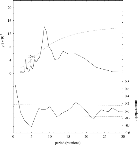
Fig. 1 : Two upper curves show the periodogram of the time series $\{S_{n}(t_{i})-\overline{S_{n}(t_{i})}\}$ (solid line) and the 95% confidence level basing on the’red noise’ (dotted line). The periodogram values are presented on the left axis. The lower curve illustrates the autocorrelation function of the same time series (solid line). The dotted lines represent two standard errors of the autocorrelation function. The dashed horizontal line shows the zero level. The autocorrelation values are shown in the right axis.

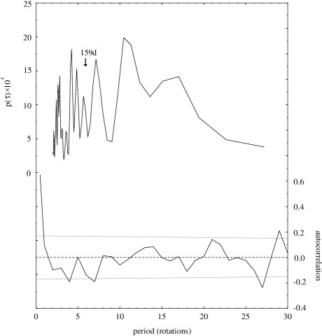
Fig. 2 : Same as in Fig. 1, but for the time series $\{S_{s}(t_{i})-\overline{S_{s}(t_{i})}\}.$ Because the statistical tests indicate that the time series is a white noise the confidence level is not marked.

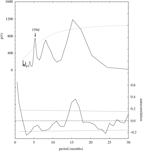
Fig. 3 : Same as in Fig. 1, but for the time series $\{R(t_{i})-\overline{R(t_{i})}\}$.

3 A method of the diagnosis of an echo-effect in the power spectrum

The method of the diagnosis of an echo-effect in the power spectrum (DE) consists in an analysis of a periodogram of a given time series computed using the BT method. The BT method bases on the cosine transform of the autocorrelation function which creates peaks which are in the periodogram, but not in the autocorrelation function.

The DE method is used for peaks which are computed by the FFT method (with high resolution) and are statistically significant. The time series of sunspot activity indexes with the spacing interval one rotation or one month contain a Markov-type persistence, which means a tendency for the successive values of the time series to ’remember’ their antecendent values. Thus, I use a confidence level basing on the ’red noise’ of Markov (Mitchell et al., 1966) for the choice of the significant peaks of the periodogram computed by the FFT method. When a time series does not contain the Markov-type persistence I apply the Fisher test and the Kolmogorov-Smirnov test at the significance level $\alpha=0.05$ (Brockwell & Davis, 1991) to verify a statistically significance of periodograms peaks. The Fisher test checks the null hypothesis that the time series is white noise agains the alternative hypothesis that the time series contains an added deterministic periodic component of unspecified frequency. Because the Fisher test tends to be severe in rejecting peaks as insignificant the Kolmogorov-Smirnov test is also used.

The DE method analyses ’raw’ estimators of the power spectrum. They are given as follows

$$\hat{S_{k}}=\frac{c_{0}}{M}+\frac{(-1)^{k}c_{M}}{M}+\frac{2}{M}\sum_{\tau=1}^{M-1}c_{\tau}\;cos(\frac{\pi k\tau}{M})$$ (1)

for $k=1,\ldots,M,$
where

$$c_{\tau}=\frac{\frac{1}{N-\tau}\sum_{i=1}^{N-\tau}{(X_{i}-\overline{X})(X_{i+\tau}-\overline{X})}}{\frac{1}{N}\sum_{i=1}^{N}{(X_{i}-\overline{X})}^{2}}$$

for $\tau=1,\ldots,M,$
$N$ is the length of the time series $\{X_{i}\}$ and $\overline{X}$ is the mean value.

The first term of the estimator $\hat{S_{k}}$ is constant. The second term takes two values (depending on odd or even $k$) which are not significant because $c_{M}\approx 0$ for large M. Thus, the third term of (1) should be analysed. Looking for intervals of $\tau$ for which $\sum_{\tau}c_{\tau}\;cos(\frac{\pi k\tau}{M})$ has the same sign and different signs one can find such parts of the function $c_{\tau}$ which create the value $\hat{S_{k}}$.

Let the set of values of the independent variable of the autocorrelation function be called $I=\{\tau:\tau=1,\ldots,M\}$ and it can be divided into the sums of disjoint sets:

$$I=\bigcup A_{i}\;\cup\;\bigcup B_{j}\;\cup\;\bigcup C_{l},$$ (2)

where
$A_{0}=\{\tau:\;c_{\tau}\cos(\frac{\pi k\tau}{M})<0\wedge 0<\tau<\frac{M}{2k}\},$

$$A_{i}=\{\tau:c_{\tau}\cos(\frac{\pi k\tau}{M})<0\wedge\frac{(2i-1)M}{2k}<\tau<$$

$$\frac{(2i+1)M}{2k}\},\quad\mbox{for}\quad i=1,\ldots,k-1,$$

$A_{k}=\{\tau:\;c_{\tau}\cos(\frac{\pi k\tau}{M})<0\wedge(2k-1)\frac{M}{2k}<\tau<M\},$
$B_{0}=\{\tau:\;c_{\tau}<0\wedge\cos(\frac{\pi k\tau}{M})<0\wedge 0<\tau<\frac{M}{2k}\},$

$$B_{j}=\{\tau:\;c_{\tau}<0\;\wedge\;\cos(\frac{\pi k\tau}{M})<0\;\wedge\;(2j-1)\frac{M}{2k}<$$

$$\quad\tau<(2j+1)\frac{M}{2k}\},\quad\mbox{for}\quad i=1,\ldots,k-1,$$ (3)

$B_{k}=\{\tau:\;c_{\tau}<0\wedge\cos(\frac{\pi k\tau}{M})<0\wedge(2k-1)\frac{M}{2k}<\tau<M\},$

$$C_{0}=\{\tau:c_{\tau}>0\wedge\cos(\frac{\pi k\tau}{M})>0\wedge 0<\tau<\frac{M}{2k}\},$$ (4)

$$C_{l}=\{\tau:\;c_{\tau}>0\;\wedge\;\cos(\frac{\pi k\tau}{M})>0\;\wedge\;(2l-1)\frac{M}{2k}<$$

$$\quad\tau<(2l+1)\frac{M}{2k}\,\},\quad\mbox{for}\quad l=1,\ldots,k-1,$$ (5)

$$C_{k}=\{\tau:\;c_{\tau}>0\wedge\cos(\frac{\pi k\tau}{M})>0\wedge(2k-1)\frac{M}{2k}<$$

$$\quad\tau<M\}.$$ (6)

Well, the set $C_{l}$ contains all integer values of $\tau$ from the interval of $((2l-1)\frac{M}{2k},(2l+1)\frac{M}{2k})$ for which the autocorrelation function and the cosinus function with the period $\Big{[}\frac{2M}{k}\Big{]}$ are positive. The index $l$ indicates successive parts of the cosinus function for which the cosinuses of successive values of $\tau$ have the same sign. However, sometimes the set $C_{l}$ can be empty. For example, for $k=13$ and $M=1000$ the set $C_{1}$ should contain all $\tau\in[38,115]$ for which $c_{\tau}>0$ and $cos(\frac{\pi k\tau}{M})>0$, but for such values of $\tau$ the values of $cos(\frac{\pi k\tau}{M})$ are negative. Thus, the set $C_{1}$ is empty.

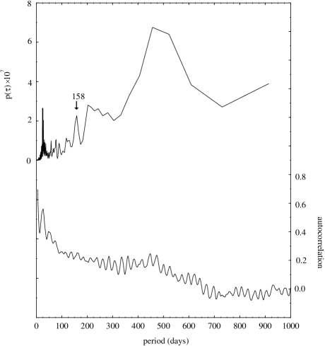
Fig. 4 : The upper curve shows the periodogram of the time series $\{S^{d}(t_{i})\}$. The periodogram values are presented on the left axis. The lower curve illustrates the autocorrelation function of the same time series. The autocorrelation values are shown in the right axis.

Let us take into consideration all sets {$A_{i}$}, {$B_{j}$} and {$C_{l}$} which are not empty. Because numberings and power of these sets depend on the form of the autocorrelation function of the given time series, it is impossible to establish them arbitrary. Thus, the sets of appropriate indexes of the sets {$A_{i}$}, {$B_{j}$} and {$C_{l}$} are called $I_{A}$, $I_{B}$ and $I_{C}$ respectively. For example the set $I_{C}$ contains all $l$ from the set $\{1,\ldots,k\}$ for which the sets $C_{l}$ are not empty.

To separate quantitatively in the estimator $\hat{S_{k}}$ the positive contributions which are originated by the cases described by the formula (5) from the cases which are described by the formula (3) the following indexes are introduced:

$$ds_{k}^{+}(l)=\frac{100\;ws_{k}^{+}(l)}{ws_{k}}\quad\mbox{for each }\quad l\in I_{C},$$

$$ds_{k}^{-}(j)=\frac{100\;ws_{k}^{-}(j)}{ws_{k}}\quad\mbox{for each }\quad j\in I_{B},$$

$$ds_{k}^{+}=\sum_{l\in I_{C}}ds_{k}^{+}(l),$$

$$ds_{k}^{-}=\sum_{j\in I_{B}}ds_{k}^{-}(j),$$

where

$$ws_{k}^{+}(l)=\sum_{\tau\in C_{l}}c_{\tau}\;cos(\frac{\pi k\tau}{M})\quad\mbox{for each}\quad l\in I_{C},$$

$$ws_{k}^{-}(j)=\sum_{\tau\in B_{j}}c_{\tau}\;cos(\frac{\pi k\tau}{M})\quad\mbox{for each}\quad j\in I_{B},$$

$$ws_{k}=\sum_{j\in I_{B}}ws_{k}^{-}(j)+\sum_{l\in I_{C}}ws_{k}^{+}(l),$$

taking for the empty sets {$B_{j}$} and {$C_{l}$} the indices $ds_{k}^{+}(l)$ and $ds_{k}^{-}(l)$ equal zero.

The index $ds_{k}^{+}(l)$ describes a percentage of the contribution of the case when $c_{\tau}$ and $cos(\frac{\pi k\tau}{M})$ are positive to the positive part of the third term of the sum (1). The index $ds_{k}^{-}(l)$ describes a similar contribution, but for the case when the both $c_{\tau}$ and $cos(\frac{\pi k\tau}{M})$ are simultaneously negative. Thanks to these one can decide which the positive or the negative values of the autocorrelation function have a larger contribution to the positive values of the estimator $\hat{S_{k}}$. When the difference $ws_{k}^{+}(l)-ws_{k}^{-}(j)$ is positive, the statement ’the $k$-th peak really exists’ can not be rejected. Thus, the following formula should be satisfied:

$$2ds_{k}^{+}-100>0.$$ (7)

Because the $k$-th peak could exist as a result of the echo-effect, it is necessary to verify the second condition:

$$\exists m\in I_{C},\quad ds_{k}^{+}(m)=\max_{l\in I_{C}}ds_{k}^{+}(l)\Rightarrow\Big{[}\frac{2M}{k}\Big{]}\in C_{m}.$$ (8)

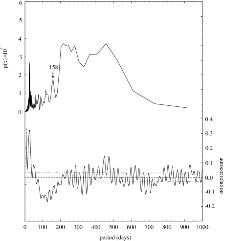
Fig. 5 : The upper curve shows the periodogram of the time series $\{S^{d}(t_{i})-\overline{S^{d}(t_{i})}\}$. The periodogram values are presented on the left axis. The lower curve illustrates the autocorrelation function of the same time series (solid line). The dotted lines represent two standard errors of the autocorrelation function. The dashed horizontal line shows the zero level. The autocorrelation values are shown in the right axis.

To verify the implication (8) firstly it is necessary to evaluate the sets $C_{l}$ for $l\in I_{C}$ of the values of $\tau$ for which the autocorrelation function and the cosine function with the period $\Big{[}\frac{2M}{k}\Big{]}$ are positive and the sets $B_{j},j\in I_{B}$ of values of $\tau$ for which the autocorrelation function and the cosine function with the period $\Big{[}\frac{2M}{k}\Big{]}$ are negative. Secondly, a percentage of the contribution of the sum of products of positive values of $c_{\tau}$ and $cos(\frac{\pi k\tau}{M})$ to the sum of positive products of the values of $c_{\tau}$ and $cos(\frac{\pi k\tau}{M})$ should be evaluated. As a result the indexes $ds_{k}^{+}(l)$ for each set $C_{l}$ where $l$ is the index from the set $I_{C}$ are obtained. Thirdly, from all sets $C_{l}$ such that $l\in I_{C}$ the set $C_{m}$ for which the index $ds_{k}^{+}(l)$ is the greatest should be chosen.

The implication (8) is true when the set $C_{m}$ includes the considered period $\Big{[}\frac{2M}{k}\Big{]}$. This means that the greatest contribution of positive values of the autocorrelation function and positive cosines with the period $\Big{[}\frac{2M}{k}\Big{]}$ to the periodogram value $\hat{S_{k}}$ is caused by the sum of positive products of $(X_{i}-\overline{X})(X_{i+\tau}-\overline{X})$ for each $\tau\in([\frac{2M}{k}]-\frac{M}{2k},[\frac{2M}{k}]+\frac{M}{2k})$.

When the implication (8) is false, the peak $\hat{S_{k}}$ is mainly created by the sum of positive products of $(X_{i}-\overline{X})(X_{i+\tau}-\overline{X})$ for each $\tau\in\Big{(}\Big{[}\frac{2M}{n}\Big{]}-\frac{M}{2k},\Big{[}\frac{2M}{n}\Big{]}+\frac{M}{2k}\Big{)}$, where $n$ is a multiple or a divisor of $k$.

It is necessary to add, that the DE method should be applied to the periodograms peaks, which probably exist because of the echo-effect. It enables one to find such parts of the autocorrelation function, which have the significant contribution to the considered peak. The fact, that the conditions (7) and (8) are satisfied, can unambiguously decide about the existence of the considered periodicity in the given time series, but if at least one of them is not satisfied, one can doubt about the existence of the considered periodicity. Thus, in such cases the sentence ’the peak can not be treated as true’ should be used.

Using the DE method it is necessary to remember about the power of the set $I$. If $M$ is too large, errors of an autocorrelation function estimation appear. They are caused by the finite length of the given time series and as a result additional peaks of the periodogram occur. If $M$ is too small, there are less peaks because of a low resolution of the periodogram. In applications $M<\frac{N}{3}$ is used. In order to evaluate the value $M$ the FFT method is used. The periodograms computed by the BT and the FFT method are compared. The conformity of them enables one to obtain the value $M$.

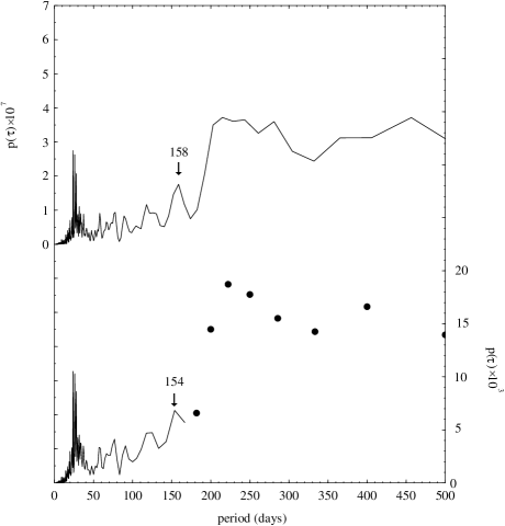
Fig. 6 : The upper curve shows the FFT periodogram of the time series $\{S^{d}(t_{i})-\overline{S^{d}(t_{i})}\}$. The FFT periodogram values are presented on the left axis. The lower curve illustrates the BT periodogram of the same time series (solid line and large black circles). The BT periodogram values are shown in the right axis.

4 Data analysis

In this paper the sunspot activity data (August 1923 - October 1933) provided by the Greenwich Photoheliographic Results (GPR) are analysed. Firstly, I consider the monthly sunspot number data. To eliminate the 11-year trend from these data, the consecutively smoothed monthly sunspot number $(\overline{R(t_{i})})$ is subtracted from the monthly sunspot number $(R(t_{i}))$ where the consecutive mean $\overline{R(t_{i})}$ is given by

$$\overline{R(t_{i})}=\frac{1}{13}\sum_{j=i-6}^{i+6}R(t_{j})\quad\mbox{for}\quad i=1,\ldots,N.$$

The values $\overline{R(t_{i})}$ for $i=1,\ldots,6$ and $i=N-6,\ldots,N$ are calculated using additional data from last six months of cycle 15 and first six months of cycle 17.

Because of the north-south asymmetry of various solar indices (Vizoso & Ballester, 1990), the sunspot activity is considered for each solar hemisphere separately. Analogously to the monthly sunspot numbers, the time series of sunspot areas in the northern and southern hemispheres with the spacing interval $\Delta t=1$ rotation are denoted. In order to find periodicities, the following time series are used:
$\{S_{n}(t_{i})-\overline{S_{n}(t_{i})}\}$ –  sunspot area fluctuations of the one rotation time interval in the northern hemisphere ($N=136$),
$\{S_{s}(t_{i})-\overline{S_{s}(t_{i})}\}$ –  sunspot area fluctuations of the one rotation time interval in the southern hemisphere ($N=136$),
$\{R(t_{i})-\overline{R(t_{i})}\}$ –  monthly sunspot number fluctuations ($N=122$).

In the lower part of Figure 1 the autocorrelation function of the time series for the northern hemisphere $\{S_{n}(t_{i})-\overline{S_{n}(t_{i})}\}$ is shown. It is easy to notice that the prominent peak falls at 17 rotations interval (459 days) and $c_{\tau}$ for $\tau\in[3,6]$ rotations ([81, 162] days) are significantly negative. The periodogram of the time series $\{S_{n}(t_{i})-\overline{S_{n}(t_{i})}\}$ (see the upper curve in Figures 1) does not show the significant peaks at $\tau=5,6$ rotations (135, 162 days), but there is the significant peak at $\tau=9$ (243 days). The peaks at $\tau=9,17$ are close to the peaks of the autocorrelation function. Thus, the result obtained for the periodicity at about $155$ days are contradict to the results obtained for the time series of daily sunspot areas (Carbonell & Ballester, 1992).

For the southern hemisphere (the lower curve in Figure 2) $c_{\tau}$ for $\tau\in[2,7]$ rotations ([54, 189] days) is not positive except $\tau=5$ (135 days) for which $c_{5}=0.02$ is not statistically significant. The upper curve in Figures 2 presents the periodogram of the time series $\{S_{s}(t_{i})-\overline{S_{s}(t_{i})}\}$. This time series does not contain a Markov-type persistence. Moreover, the Kolmogorov-Smirnov test and the Fisher test do not reject a null hypothesis that the time series is a white noise only. This means that the time series do not contain an added deterministic periodic component of unspecified frequency.

The autocorrelation function of the time series $\{R(t_{i})-\overline{R(t_{i})}\}$ (the lower curve in Figure 3) has only one statistically significant peak for $\tau=16$ months (480 days) and negative values for $\tau\in[3,13]$ months ([90, 390] days). However, the periodogram of this time series (the upper curve in Figure 3) has two significant peaks the first at 15.2 and the second at 5.3 months (456, 159 days). Thus, the periodogram contains the significant peak, although the autocorrelation function has the negative value at $\tau=5$ months.

To explain these problems two following time series of daily sunspot areas are considered:
$\{S^{d}(t_{i})\}$ –  daily sunspot areas in the whole solar disk ($N=3653$),
$\{S^{d}(t_{i})-\overline{S^{d}(t_{i})}\}$ –  daily sunspot area fluctuations,
where

$$\overline{S^{d}(t_{i})}=\frac{1}{365}\sum_{j=i-182}^{i+182}S^{d}(t_{j})\quad\mbox{for}\quad i=1,\ldots,N.$$ (9)

The values $\overline{S^{d}(t_{i})}$ for $i=1,\ldots,182$ and $i=N-182,\ldots,N$ are calculated using additional daily data from the solar cycles 15 and 17.

Fig. 7 : Autocorrelation function of the time series $\{S^{d}(t_{i})-\overline{S^{d}(t_{i})}\}$ and the cosine function for $k=13$ (the period at about 154 days). The horizontal line (dotted line) shows the zero level. The vertical dotted lines evaluate the intervals where the sets $A_{i},B_{j},C_{l}$ (for $i,j,l=1,\ldots,k$) are searched. The percentage values show the index $ds_{k}^{+}(l)$ for each $C_{l}$ for the time series $\{S^{d}(t_{i})-\overline{S^{d}(t_{i})}\}$ (in parentheses for the time series $\{S^{d}(t_{i})\}$). In the right bottom corner the values of $ds_{k}^{+}(l)$ for the time series $\{S^{d}(t_{i})-\overline{S^{d}(t_{i})}\}$, for $\tau=501,\ldots,1000$ are written.

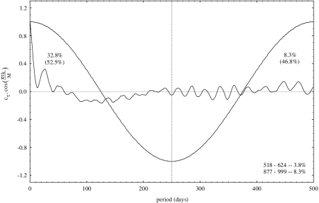
Fig. 8 : Same as in Figure 7, but for $k=4$ (the 500-day period )

The comparison of the functions $c_{\tau}$ of the time series $\{S^{d}(t_{i})\}$ (the lower curve in Figure 4) and $\{S^{d}(t_{i})-\overline{S^{d}(t_{i})}\}$ (the lower curve in Figure 5) suggests that the positive values of the function $c_{\tau}$ of the time series $\{S^{d}(t_{i})\}$ in the interval of $[61,209]$ days could be caused by the 11-year cycle. This effect is not visible in the case of periodograms of the both time series computed using the FFT method (see the upper curves in Figures 4 and 5) or the BT method (see the lower curve in Figure 6). Moreover, the periodogram of the time series $\{S^{d}(t_{i})-\overline{S^{d}(t_{i})}\}$ has the significant values at $\tau=117,158,203$ days, but the autocorrelation function is negative at these points. Carbonell & Ballester (1992) showed that the Lomb-Scargle periodograms for the both time series (see Carbonell & Ballester (1992), Figures 7 a-c) have a peak at 158.8 days which stands over the FAP level by a significant amount. Using the DE method the above discrepancies are obvious. To establish the $M$ value the periodograms computed by the FFT and the BT methods are shown in Figure 6 (the upper and the lower curve respectively). For $M=1000$ and for periods less than 166 days there is a good comformity of the both periodograms (but for periods greater than 166 days the points of the BT periodogram are not linked because the BT periodogram has much worse resolution than the FFT periodogram (no one know how to do it)). For $M=1000$ and $\tau=154$ the value of $k$ is 13 ($\Big{[}\frac{2M}{k}\Big{]}=153$). The inequality (7) is satisfied because $2ds_{k}^{+}-100=26\%$. This means that the value of $\hat{S_{13}}$ is mainly created by positive values of the autocorrelation function. The implication (8) needs an evaluation of the greatest value of the index $ds_{k}^{+}(l)$ where $l\in I_{C}$, but the solar data contain the most prominent period for $\tau=27$ days because of the solar rotation. Thus, although $ds_{k}^{+}(0)=\max_{l\in I_{C}}ds_{k}^{+}(l)$ for each $k<13$, all sets $C_{l}$ (see (5) and (6)) without the set $C_{0}$ (see (4)), which contains $\tau\in[0,38]$, are considered. This situation is presented in Figure 7. In this figure two curves $y=cos\frac{\pi k\tau}{M}$ and $y=c_{\tau}$ are plotted. The vertical dotted lines evaluate the intervals where the sets $A_{i},B_{j},C_{l}$ (for $i,~{}j,~{}l=1,\ldots,k$) are searched. For such $C_{l}$ two numbers are written: in parentheses the value of $ds_{k}^{+}(l)$ for the time series $\{S^{d}(t_{i})\}$ and above it the value of $ds_{k}^{+}(l)$ for the time series $\{S^{d}(t_{i})-\overline{S^{d}(t_{i})}\}$. To make this figure clear the curves are plotted for the set $\{\tau:\tau=1,\ldots,500\}$ only. (In the right bottom corner information about the values of $ds_{k}^{+}(l)$ for the time series $\{S^{d}(t_{i})-\overline{S^{d}(t_{i})}\}$, for $\tau=501,\ldots,1000$ are written.) The implication (8) is not true, because $ds_{k}^{+}(m)=14.8\%$ for $m=6$. Therefore, $\Big{[}\frac{2M}{k}\Big{]}=153\notin C_{6}=[423,500]$. Moreover, the autocorrelation function for $\tau\in[115,192]$ is negative and the set $C_{2}$ is empty. Thus, $ds_{k}^{+}(2)=0\%$. On the basis of these information one can state, that the periodogram peak at $\tau\approx 154$ days of the time series $\{S^{d}(t_{i})-\overline{S^{d}(t_{i})}\}$ exists because of positive $c_{\tau}$, but for $\tau$ from the intervals which do not contain this period. Looking at the values of $ds_{k}^{+}(l)$ of the time series $\{S^{d}(t_{i})\}$, one can notice that they decrease when $\tau$ increases until $\tau=346$. This indicates, that when $\tau$ increases, the contribution of the 11-year cycle to the peaks of the periodogram decreases. An increase of the value of $ds_{k}^{+}(l)$ is for $l=6$ for the both time series, although the contribution of the 11-year cycle for the time series $\{S^{d}(t_{i})\}$ is insignificant. Thus, this part of the autocorrelation function ($ds_{k}^{+}(6)=\max_{l=1,\ldots,s}ds_{k}^{+}(l)$ for the time series $\{S^{d}(t_{i})-\overline{S^{d}(t_{i})}\}$) influences the $k$-th peak of the periodogram. This suggests that the periodicity at about 155 days is a harmonic of the periodicity from the interval of $[400,500]$ days.

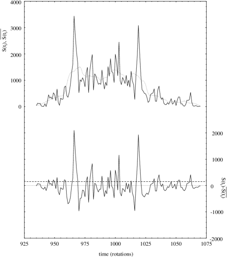
Fig. 9 : Two upper curves show sunspot areas of the one rotation time interval in the whole solar disk $S(t_{i})$ (solid line) and consecutively smoothed sunspot areas of the one rotation time interval $\overline{S(t_{i})}$ (dotted line). Both indexes are presented on the left axis. The lower curve illustrates fluctuations of the sunspot areas $S(t_{i})-\overline{S(t_{i})}$. The dotted and dashed horizontal lines represent levels zero and $p$ respectively. The fluctuations are shown on the right axis.

The described reasoning can be carried out for other values of the periodogram. For example, the condition (8) is not satisfied for $k=8,9,10$ (250, 222, 200 days). Moreover, the autocorrelation function at these points is negative. These suggest that there are not a true periodicity in the interval of [200, 250] days. It is difficult to decide about the existence of the periodicities for $k=6$ (333 days) and $k=7$ (286 days) on the basis of above analysis. The implication (8) is not satisfied for $k=7$ and the condition (7) is not satisfied for $k=6$, although the function $c_{\tau}$ of the time series $\{S^{d}(t_{i})-\overline{S^{d}(t_{i})}\}$ is significantly positive for $\tau=286,333$. The conditions (7) and (8) are satisfied for $k=4$ (Figure 8) and $k=5$. Therefore, it is possible to exist the periodicity from the interval of $[400,500]$ days. Similar results were also obtained by Lean (1990) for daily sunspot numbers and daily sunspot areas. She considered the means of three periodograms of these indexes for data from $N=31$ years and found statistically significant peaks from the interval of $[400,500]$ (see Lean (1990), Figure 2). Krivova & Solanki (2002) studied sunspot areas from 1876-1999 and sunspot numbers from 1749-2001 with the help of the wavelet transform. They pointed out that the 154-158-day period could be the third harmonic of the 1.3-year (475-day) period. Moreover, the both periods fluctuate considerably with time, being stronger during stronger sunspot cycles. Therefore, the wavelet analysis suggests a common origin of the both periodicities. This conclusion confirms the DE method result which indicates that the periodogram peak at $\tau=154$ days is an alias of the periodicity from the interval of $[400,500]$.

5 The periodicity at about 155 days during the maximum activity period

In order to verify the existence of the periodicity at about 155 days I consider the following time series:
$\{S(t_{i})-\overline{S(t_{i})}\}$ –  sunspot area fluctuations of the one rotation time interval in the whole solar disk ($N=136$),
$\{S^{d}_{n}(t_{i})-\overline{S^{d}_{n}(t_{i})}\}$ –  daily sunspot area fluctuations in the northern hemisphere from the maximum activity period (January 1925 - December 1930, $N=1478$),
$\{S^{d}_{s}(t_{i})-\overline{S^{d}_{s}(t_{i})}\}$ –  daily sunspot area fluctuations in the southern hemisphere from the maximum activity period ($N=1478$).

The value $\overline{S(t_{i})}$ is calculated analogously to $\overline{R(t_{i})}$ (see Sect. 4). The values $\overline{S^{d}_{n}(t_{i})}$ and $\overline{S^{d}_{s}(t_{i})}$ are evaluated from the formula (9). In the upper part of Figure 9 the time series of sunspot areas $(S(t_{i}))$ of the one rotation time interval from the whole solar disk and the time series of consecutively smoothed sunspot areas $(\overline{S(t_{i})}=\frac{1}{13}\sum_{j=i-6}^{i+6}{S(t_{i})})$ are showed. In the lower part of Figure 9 the time series of sunspot area fluctuations $\{S(t_{i})-\overline{S(t_{i})}\}$ is presented. On the basis of these data the maximum activity period of cycle 16 is evaluated. It is an interval between two strongest fluctuations e.a. $J=[966,1019]$ rotations. The length of the time interval $J$ is 54 rotations. If the about $155$-day (6 solar rotations) periodicity existed in this time interval and it was characteristic for strong fluctuations from this time interval, 10 local maxima in the set of $F_{i}=S(t_{i})-\overline{S(t_{i})}$ would be seen. Then it should be necessary to find such a value of p for which $F_{i}>p$ for $i\in J$ and the number of the local maxima of these values is 10. As it can be seen in the lower part of Figure 9 this is for the case of $p=150$ (in this figure the dashed horizontal line is the level of $F_{i}=150$). Figure 10 presents nine time distances among the successive fluctuation local maxima and the horizontal line represents the 6-rotation periodicity. It is immediately apparent that the dispersion of these points is 10 and it is difficult to find even few points which oscillate around the value of 6. Such an analysis was carried out for smaller and larger $p$ and the results were similar. Therefore, the fact, that the about $155$-day periodicity exists in the time series of sunspot area fluctuations during the maximum activity period is questionable.

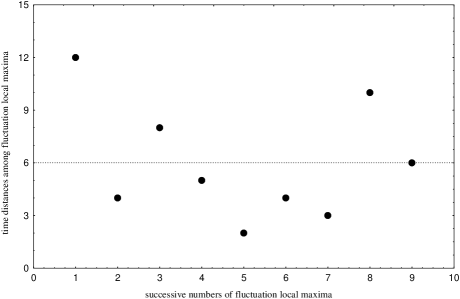
Fig. 10 : Nine time distances among the successive local maxima of the values of $F_{i}>p$. The horizontal line represents the 6-rotation (162-day) period.

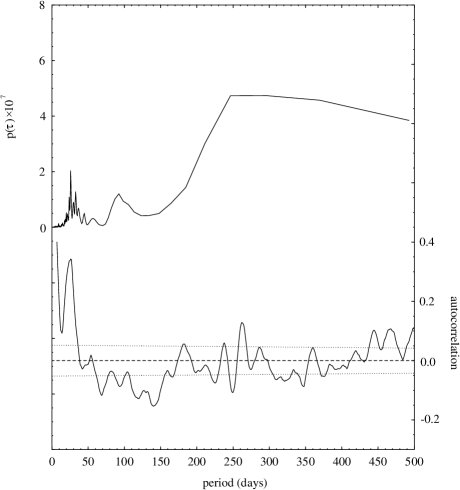
Fig. 11 : Same as in Fig. 5, but for the time series $\{S^{d}_{n}(t_{i})-\overline{S^{d}_{n}(t_{i})}\}.$

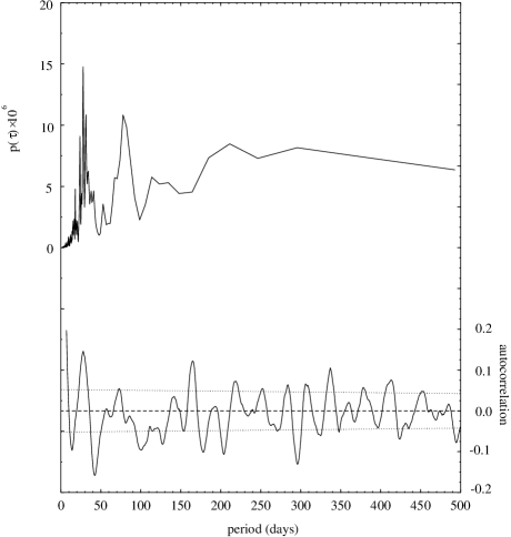
Fig. 12 : Same as in Fig. 5, but for the time series $\{S^{d}_{s}(t_{i})-\overline{S^{d}_{s}(t_{i})}\}.$

To verify again the existence of the about $155$-day periodicity during the maximum activity period in each solar hemisphere separately, the time series $\{S_{n}(t_{i})-\overline{S_{n}(t_{i})}\}$ and $\{S_{s}(t_{i})-\overline{S_{s}(t_{i})}\}$ were also cut down to the maximum activity period (January 1925–December 1930). The comparison of the autocorrelation functions of these time series with the appriopriate autocorrelation functions of the time series $\{S_{n}(t_{i})-\overline{S_{n}(t_{i})}\}$ and $\{S_{s}(t_{i})-\overline{S_{s}(t_{i})}\}$, which are computed for the whole 11-year cycle (the lower curves of Figures 1 and 2), indicates that there are not significant differences between them especially for $\tau$=5 and 6 rotations (135 and 162 days)). This conclusion is confirmed by the analysis of the time series $\{S^{d}_{n}(t_{i})-\overline{S^{d}_{n}(t_{i})}\}$ for the maximum activity period. The autocorrelation function (the lower curve of Figure 11) is negative for the interval of [57, 173] days, but the resolution of the periodogram is too low to find the significant peak at $\tau=158$ days. The autocorrelation function gives the same result as for daily sunspot area fluctuations from the whole solar disk ($\{S^{d}(t_{i})-\overline{S^{d}(t_{i})}\}$) (see also the lower curve of Figures 5). In the case of the time series $\{S_{s}(t_{i})-\overline{S_{s}(t_{i})}\}$ $c_{5}$ is zero for the fluctuations from the whole solar cycle and it is almost zero ($c_{\tau}=0.02$) for the fluctuations from the maximum activity period. The value $c_{6}$ is negative. Similarly to the case of the northern hemisphere the autocorrelation function and the periodogram of southern hemisphere daily sunspot area fluctuations from the maximum activity period $\{S^{d}_{s}(t_{i})-\overline{S^{d}_{s}(t_{i})}\}$ are computed (see Figure 12). The autocorrelation function has the statistically significant positive peak in the interval of [155, 165] days, but the periodogram has too low resolution to decide about the possible periodicities. The correlative analysis indicates that there are positive fluctuations with time distances about $155$ days in the maximum activity period.

The results of the analyses of the time series of sunspot area fluctuations from the maximum activity period are contradict with the conclusions of Lean (1990). She uses the power spectrum analysis only. The periodogram of daily sunspot fluctuations contains peaks, which could be harmonics or subharmonics of the true periodicities. They could be treated as real periodicities. This effect is not visible for sunspot data of the one rotation time interval, but averaging could lose true periodicities. This is observed for data from the southern hemisphere. There is the about $155$-day peak in the autocorrelation function of daily fluctuations, but the correlation for data of the one rotation interval is almost zero or negative at the points $\tau=5$ and 6 rotations. Thus, it is reasonable to research both time series together using the correlative and the power spectrum analyses.

6 Conclusion

The following results are obtained:

1. A new method of the detection of statistically significant peaks of the periodograms enables one to identify aliases in the periodogram.

2. Two effects cause the existence of the peak of the periodogram of the time series of sunspot area fluctuations at about $155$ days: the first is caused by the 27-day periodicity, which probably creates the 162-day periodicity (it is a subharmonic frequency of the 27-day periodicity) and the second is caused by statistically significant positive values of the autocorrelation function from the intervals of $[400,500]$ and $[501,1000]$ days.

3. The existence of the periodicity of about $155$ days of the time series of sunspot area fluctuations and sunspot area fluctuations from the northern hemisphere during the maximum activity period is questionable.

4. The autocorrelation analysis of the time series of sunspot area fluctuations from the southern hemisphere indicates that the periodicity of about 155 days exists during the maximum activity period.

References

- Akioka et al. ( 1987) Akioka, M., Kubota, J., Suzuki, M., Ichimoto, K., & Tohmura, I. 1987, Sol. Phys., 112, 313
- Anderson (1971) Anderson, T. W., 1971, ”The statistical analysis of time series”, John Wiley & Sons: New York
- Bai (1987a) Bai, T. 1987a, Astrophys. J., 318, L85
- Bai (1992) Bai, T. 1992, Astrophys. J., 388, L69
- Bai & Cliver (1990) Bai, T., & Cliver, E. W. 1990, Astrophys. J., 363, 299
- Bai & Sturrock (1987) Bai, T. & Sturrock, P. A. 1987, Nature, 327, 601
- Blackman & Tukey (1958) Blackman, R. B., & Tukey J. W., 1958, ”The measurment of power spectra”, Dower, Inc., New York
- Bogart & Bai (1985) Bogart, R. S. & Bai, T., 1985, Astrophys. J., 299, L51
- Brockwell & Davis (1991) Brockwell, P. J., & Davis, R. A., 1991, ”Time series: Theory and Methods”, Springer: New York