Universal Randomness

Abstract

During last two decades it has been discovered that the statistical properties of a number of microscopically rather different random systems at the macroscopic level are described by the same universal probability distribution function which is called the Tracy-Widom (TW) distribution. Among these systems we find both purely methematical problems, such as the longest increasing subsequences in random permutations, and quite physical ones, such as directed polymers in random media or polynuclear crystal growth. In the extensive Introduction we discuss in simple terms these various random systems and explain what the universal TW function is. Next, concentrating on the example of one-dimensional directed polymers in random potential we give the main lines of the formal proof that fluctuations of their free energy are described the universal TW distribution. The second part of the review consist of detailed appendices which provide necessary self-contained mathematical background for the first part.

Contents

	I. Introduction
	A. Combinatorics
	B. Polynuclear crystal growth
	C. Directed polymers
	D. Replica method
	E. Tracy-Widom distribution function
	II. Directed polymers and one-dimensional quantum bosons
	III. Solution of the one-dimensional directed polymers problem
	IV. Conclusions
	Appendix A: Quantum bosons with repulsive interactions
	1. Eigenfunctions
	2. Othonormality
	Appendix B: Quantum bosons with attractive interactions
	1. Ground state
	2. Eigenfunctions
	3. Othonormality
	4. Propagator
	Appendix C: The Airy function integral relations
	Appendix D: Fredholm determinant with the Airy kernel
	and the Tracy-Widom distribution

I Introduction

Everyone knows the Gaussian distribution function. Whenever we are dealing with a system containing independent random parameters, its macroscopic characteristics (according to the central limit theorem) are described by the Gaussian distribution. This kind of universal behavior is trivial, and not so much interesting. On the other hand, every non-trivial system usually requires individual consideration, and although there are lot of universal macroscopic properties among microscopically different systems (e.g. scaling and critical phenomena at the phase transitions) until very recently no one would expect to have a universal function (different from the Gaussian one) which would describe macroscopic statistical properties of a whole class of non-trivial random systems.

Originally the solution of Tracy and Widom Tracy-Widom were devoted to rather specific mathematical problem, namely the distribution function of the largest eigenvalue of $N\times N$ Hermitian matrices (Gaussian Unitary Ensemble (GUE)) in the limit $N\to\infty$. Nowadays we have got rather comprehensive list of various systems (both purely mathematical and physical) whose macroscopic statistical properties are described by the same universal Tracy-Widom (TW) distribution function. These systems are: the longest increasing subsequences (LIS) model LIS (Section I.A) zero-temperature lattice directed polymers with geometric disorder DP_johansson the polynuclear growth (PNG) system PNG_Spohn , (Section I.B) the oriented digital boiling model oriented_boiling , the ballistic decomposition model ballistic_decomposition , the longest common subsequences (LCS) LCS , the one-point distribution of the solutions of the KPZ equation KPZ (which describes the motion of an interface separating two homogeneous bulk phases) in the long time limit KPZ-TW1 ; KPZ-TW2 , and finally finite temperature directed polymers in random potentials with short-range correlations Dotsenko1 ; Dotsenko2 ; Dotsenko3 ; LeDoussal . It should be noted that directed polymers in a quenched random potential have been the subject of intense investigations during the past three decades (see e.g. hh_zhang_95 ). Diverse physical systems such as domain walls in magnetic films lemerle_98 , vortices in superconductors blatter_94 , wetting fronts on planar systems wilkinson_83 , or Burgers turbulence burgers_74 can be mapped to this model, which exhibits numerous non-trivial features deriving from the interplay between elasticity and disorder.

The rest of this Introduction is devoted to the discussion of several random statistical systems with explanations in very simple terms of what the TW distribution describes in them. Namely, we will consider the combinatorial model of the longest increasing subsequences (section I.A), the polynuclear crystal growth model (section I.B), and one-dimensional directed polymers in random potential (section I.C). Besides in section I.D the main ides of the replica method (used in the present approach) will be described, and finally in section I.E the definition and the main properties of the TW distribution function will be given.

Sections II and III are devoted to the exact solution of the one-dimensional directed polymers problem. In particular, in section II the main ideas of this solution as well as its methodological tools are described. Section III contains the main lines of the derivation of the TW distribution function for the free energy fluctuations in one-dimensional directed polymers with $\delta$-correlated random potential. The second part of this review contains several technical appendices containing all necessary mathematical tools (used in the previous sections) which hopefully makes the whole paper to be self-contained.

I.1 Combinatorics

We start with purely mathematical ”toy” model which, as we will see later, is closely related with physical problems of polynuclear crystal growth (section I.B) and one-dimensional directed polymers (section I.C). This combinatorial problem of statistical properties of the longest increasing subsequences (LIS) was formulated long time ago by Ulam Ulam , and hence it is often called the Ulam’s problem. Let us consider a sequence of $N$ integers $\{1,2,...,N\}$. Then, for an arbitrary permutation of these integers we have to find all possible increasing subsequences, and among them the length $l_{N}$ of the longest ones should be defined. As an example let us consider the case $N=11$ and take a particular permutation

$$\{3,5,10,1,9,6,8,4,7,11,2\}.$$ (1.1)

This permutation exhibits many different increasing subsequences (such as $\{3,5,10,11\}$, $\{1,9,11\}$ etc.), and among them the longest ones are $\{3,5,6,7,11\}$ and $\{3,5,6,8,11\}$. In other words, for this particular permutation $l_{N}=5$. Simple graphical representation of this permutation problem is shown in Figure 1. Here the set of $11$ bold dots inside the $(12\times 12)$ square represents the permutation, eq.(1.1): for every integer in the $x$ direction one associates one and only one permuted integer in the $y$ direction (for $x=1$ one gets $y=3$, for $x=2$ one gets $y=5$, etc.). All possible increasing subsequences of this particular permutation are obtained by drawing all possible directed paths connecting the origin $(0,0)$ with the right up corner $(12,12)$ of this square, which are passing over the internal bold dots. Directed path means that only “right-and-up“ movements are allowed when going from one dot to another. For example, from the point $(6,6)$ one can jump only to the points $(7,8)$, $(9,7)$ and $(10,11)$. In other words, when going from the origin to the right up corner $(12,12)$ both $x$ and $y$ coordinates can only increase at every step. In terms of these rule, the longest increasing subsequence is described by the directed path which goes over the maximum possible number of dots. Note that for a given permutation the longest increasing subsequence is not necessary unique. In the considered example in addition to the subsequence $\{3,5,6,7,11\}$ shown in Figure 1 by the dotted line, there exist another one namely $\{3,5,6,8,11\}$.

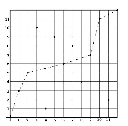
Figure 1: Geometrical representation of the permutation, eq.(1.1), for $N=11$. The dotted line corresponds the longest increasing subsequence $\{3,5,6,7,11\}$

Considering all $N!$ possible permutations with equal probability one find that the length $l_{N}$ varies from permutation to permutation being the random variable. The question is what are the statistical properties of the random quantity $l_{N}$. First it has been shown that in the limit of large $N$, the average value of the longest increasing subsequence, $\overline{l_{N}}$, is proportional to $\sqrt{N}$, namely $\overline{l_{N}}\sim c\sqrt{N}$, where the constant $c=2$ Vershik-Kerov . Moreover, in the limit $N\to\infty$, the quantity $l_{N}$ in order $\sqrt{N}$ is selfaveraging: $\lim_{N\to\infty}l_{N}/\sqrt{N}\,=\,2$ (in other words, the distribution function of the ratio $l_{N}/\sqrt{N}$ in the limit $N\to\infty$ shrinks to the $\delta$-function).

Note that at the qualitative level one can easily understand why the typical value of $l_{N}$ must be proportional to $\sqrt{N}$. Indeed, for large $N$ a generic permutation of the numbers $\{1,2,...,N\}$ in terms of the permutation matrix of Figure 1 will be represented by a uniform distribution of $N$ dots inside the $N\times N$ square. Thus the density of the dots will be proportional to $1/N$ while the typical distance between neighboring dots must be proportional to $\sqrt{N}$. It means that the typical number of dots on a diagonal-like path of the length $\sim N$ must be proportional to $N/\sqrt{N}=\sqrt{N}$.

However, the main interest in this system is not the typical value of the longest increasing subsequences, but their fluctuations. Recently it has been shown LIS ; Aldous that in the limit of large $N$ the fluctuations of $l_{N}$ scale as $N^{1/6}$, namely,

$$l_{N}\;\simeq\;2\sqrt{N}\,+\,N^{1/6}\,s$$ (1.2)

where the random quantity $s$ is described by the universal $N$-independent distribution function $P_{TW}(s)$, which is the Tracy-Widom distribution (see section I.E):

$$\lim_{N\to\infty}\mbox{Prob}\biggl{(}\frac{l_{N}-2\sqrt{N}}{N^{1/6}}=s\biggr{)}\;=\;P_{TW}(s)$$ (1.3)

It turns out that the above purely mathematical ”toy” model is equivalent to the physical model of (2+1)-dimensional polynuclear crystal growth, where the TW distribution describes the fluctuations of the number of the crystal mono-layers (see next subsection).

I.2 Polynuclear crystal growth

It turns out that the mathematical ”toy” model considered above is equivalent to the physical model of the crystal growth with randomly located nucleation centers. This is the model of polynuclear crystal growth (PNG) which describes the growth of the two-dimensional crystal monolayers in (2+1) dimensions.

Let us consider again Figure 1 where the bold dots will be assumed to represent the nucleation centers. The crystal layers growth takes place in the vertical direction (toward the reader) according to the following rules. From each nucleation center we draw the monolayer level step straight line in the horizontal direction to the right and in the vertical direction up, until these lines meet with the other lines starting from the other centers. In this way we are getting the monolayer ”terraces” which mount from the left-down to the right-up corner of the square. (see Figure 2).

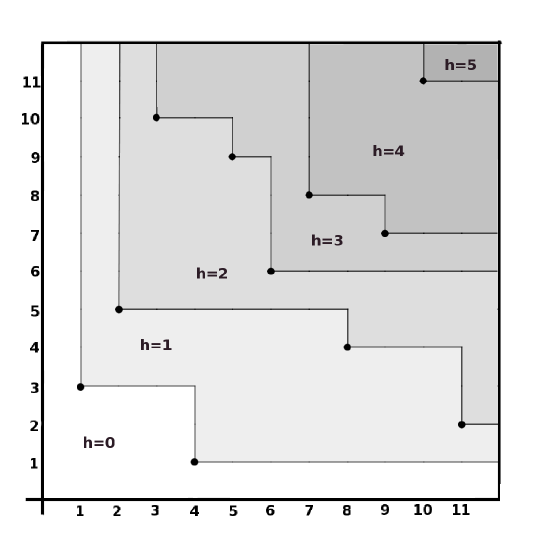
Figure 2: (2+1)-dimensional crystal terraces with the ”nucleation centers” corresponding to the permutation model of Figure 1

One can easily see that for a given random positions of the nucleation centers (for a given permutation in the previous LIS problem) the number of terraces $h_{N}$ is just equal to the longest increasing permutation $l_{N}$ in the combinatorial problem considered in the previous subsection. For a given value of $N$, depending on the actual configurations of the nucleation centers inside the $N\times N$ square, the number of the monolayer terraces is the random quantity, and in the limit $N\to\infty$ its statistics is described by the TW distribution, eq.(1.3) PNG_Spohn . At present the study of various modifications of PNG model formulated above is the vast field of research (see e.g. Ferrari ). It is also interesting to note that quite recently the existence of TW distribution in the PNG-like systems has been confirmed experimentally takeuchi .

I.3 Directed polymers

It is clear that when the size of the square $N$ is large the presence of the background lattice is not essential. In this case instead of considering the problem in terms of permutations one can introduce a homogeneous distribution of dots inside continuous square (Figure 3).

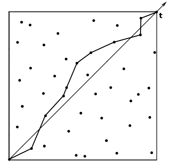
Figure 3: Directed path through randomly distributed dots

Let us introduce here the diagonal ”time” axes which goes from the origin (left down corner) to the right up corner of the square. The directed polymer here is the line which starts at the origin and arrives to the right up corner ”jumping” over the dots in such a way that its time coordinates increases at every jump. For a given (random) configuration of dots among many possible directed polymer trajectories we have to choose the ones which contains the maximum number of dots. In this formulation the problem of statistics of the length of such directed polymers looks somewhat different from the LIS problem considered above. It can be shown however, that in the limit of large times $t$ and large $N$ these two problems become equivalent LIS . For a given (fixed) density $\rho$ of dots instead of the total number of dots $N$ one can measure the length $l(t)$ of the polymer in terms of the size of the square $t$. Since $\rho=2N/t^{2}$, assuming that $\rho$ is a parameter which is of the order of one, we note that $t\propto\sqrt{N}$. In this case we find that the fluctuations of the length of the polymers scales as $t^{1/3}$, and instead of eq.(1.3) we get

$$\lim_{t\to\infty}\mbox{Prob}\biggl{(}\frac{l(t)-\sqrt{2\rho}\,t}{t^{1/3}}=s\biggr{)}\;=\;P_{TW}(s)$$ (1.4)

In other words in the thermodynamic limit, $t\to\infty$ all the systems considered above appear to be equivalent to each other which doesn’t look so much surprising if we compare Figures 1-3.

In statistical physics one defines random directed polymers in somewhat different way. Let us introduce a square lattice in which discrete ”time” $t=1,2,...,L$ is now horizontal (Figure 4). The vertical direction is described by the discrete parameter $\phi=0,\pm 1,\pm 2,...,\pm M$. At every lattice site $(\phi,t)$ we place random quantities (random potential) $V(\phi,t)$ and assume that they are described by independent Gaussian distributions:

$${\cal P}[{\bf V}]\;=\;\prod_{\phi,t}\sqrt{\frac{1}{2\pi u}}\exp\Bigl{(}-\frac{1}{2u}V^{2}(\phi,t)\Bigr{)}$$ (1.5)

The parameter $u$ defines the typical strength of the random potentials $V(\phi,t)$, which according to eq.(1.5) are uncorrelated

$$\overline{V(\phi,t)\,V(\phi^{\prime},t^{\prime})}\;=\;u\,\delta_{\phi,\phi^{\prime}}\,\delta_{t,t^{\prime}}$$ (1.6)

and have zero mean value, $\overline{V(\phi,t)}=0$ (the horizontal line denotes the averaging with the distribution, eq.(1.5)).

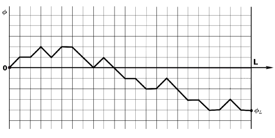
Figure 4: Directed polymer on a square lattice

The directed polymer here is the path which starts at the origin and goes over the lattice sites to the right end of the system. At every time step, $t\to t+1$ the polymer trajectory $\phi(t)$, can deviate up or down by one step or may not deviate at all: $\phi(t+1)=\phi(t)+\sigma(t+1)$, where $\sigma=\pm 1,0$. Assuming that the polymer is a kind of elastic string we can introduce ”elastic” (positive) energy $\propto\bigl{[}\phi(t+1)-\phi(t)\bigr{]}^{2}$ for every polymer’s deviation. In this way for a given trajectory $\phi(t)$ we can associate the following energy:

$$H[\phi(t)]\;=\;\sum_{t=1}^{L-1}\Bigl{[}\frac{1}{2}\bigl{[}\phi(t+1)-\phi(t)\bigr{]}^{2}+V(\phi(t),t)\Bigr{]}$$ (1.7)

This expression contains two competing contributions: the first (elastic) terms are trying to make the trajectory as horizontal as possible, while the second ones are forcing the trajectory to deviate in the search for the most negative values of the random potentials. For a given (random) configuration of the potentials $V(\phi,t)$ the optimal trajectory $\phi_{*}(t)$ is defined by the minimum of the total energy, eq.(1.7),

$$E(L)\;=\;\min_{\phi(t)}\Biggl{\{}\sum_{t=1}^{L-1}\Bigl{[}\frac{1}{2}\bigl{[}\phi(t+1)-\phi(t)\bigr{]}^{2}+V(\phi(t),t)\Bigr{]}\Biggr{\}}$$ (1.8)

Being the function of the random potential $V(\phi,t)$ this quantity is also random, and it could be considered as the distant analog of the (random) length of the directed polymers in the previous example shown in Figure 3. An essential difference is that in this latter case the elastic terms are absent, while the (negative) contribution of the potential energy is associated with a fixed energy $V_{0}$ carried by the dots which (unlike the Gaussian random potentials $V(\phi,t)$) are geometrically random. One more important difference is that unlike the directed polymer in Figure 4, which is defined by the local in space one-step wandering, the trajectory in Figure 3 can jump any distance from dot to dot (not necessary between neighboring dots). Thus, a priori there are no reasons to expect that these two quantities, $E(L)$, eq.(1.8), and $l(t)$ in the example of Figure 3 would have the same statistical properties. If, nevertheless, we would suppose that at least in the thermodynamic limit, $t\sim L\to\infty$, these two types of systems become equivalent we would have to expect that $E(L)\;\simeq\;f_{0}\,L\;+\;L^{1/3}s$, where $f_{0}$ is the bulk (selfaveraging) energy density and the random parameter $s$ is described by $L$-independent TW distribution function.

The system defined by the Hamiltonian (1.7) is the usual one-dimensional statistical system containing quenched disorder. The fact that the leading contribution to its ground state energy $E(L)$ is proportional to the system size $L$ can be explained in very simple way. Indeed, in the first approximation, to minimize the energy at every time step among three possible options (”up”,”horizontal” and ”down”) the trajectory of Figure 4 can choose the site where the value of the random potential $V(\phi,t)$ is lower (in this approximation we neglect the presence of non-local phenomena when the optimal trajectory chooses locally unfavorable option to gain globally more favorable energy). In this way the second term in eq.(1.7) provides the contribution which is proportional to $-\sqrt{u}\,L$ (and not $\sqrt{uL}$, as it would be for an arbitrary trajectory $\phi(t)$). Since the contribution of the first (elastic) term in eq.(1.7) is also proportional to $L$, we find that in the leading order in $L$, the energy of the optimal trajectory $E(L)\;\simeq\;-(const)\,L$, and moreover, we can be sure that this contribution is negative since the energy of the optimal trajectory in the absence on the random potentials is zero (it is just the straight horizontal line), while the presence of the random potential can only lower the energy. On the other hand the fact that finite-size corrections in this system are of order $L^{1/3}$ (and not of order $L^{1/2}$, as one could naively expect) is highly non-trivial phenomenon which is very difficult to explain in simple terms.

The lattice model as it is introduced above, eqs.(1.7)-(1.8), is essentially the zero-temperature system, as we are dealing here with the optimal (global minimum) trajectories only. It is clear that the search for the global minimum configurations in eq.(1.8) is highly non-trivial task, as it can not be done via the local in time algorithms. On the other hand, as it often happens, one can make life much easier if one consider more general (i.e. more complicated) problem. Namely, let us introduce finite temperature $T$ in the system so that in addition to the quenched disorder fluctuations we would have the contributions of the thermal fluctuations produced by the trajectories away from the global minima ones. In terms of this generalization instead of the global minimum energy $E(L)$, eq.(1.8), we would get the free energy:

$$F(L,T)\,=\,-T\ln\Bigl{[}\sum_{\phi(t)}\exp\Bigl{(}-\frac{1}{T}H[\phi(t)]\Bigr{)}\Bigr{]}$$ (1.9)

where the expression under the logarithm is the partition function in which the summation goes over all trajectories starting at the origin. In the case the global minimum trajectory is unique (which is usually the case in the large system) the energy defined in eq.(1.8) is obtained by taking the zero temperature limit: $E(L)\,=\,\lim_{T\to 0}F(L,T)$. The finite temperature lattice model defined by eqs.(1.7),(1.9) is sufficiently simple for numerical investigations (see e.g. Krug ) which in particular allows to demonstrate the existence of the free energy fluctuations scaling $\sim L^{1/3}$. On the other hand, the problem defined on a lattice is very hard for analytical studies. Since the phenomena of interest are taking place at large system sizes, one may hope that it would be sufficient to consider the system in the continuous limit where the presence of a lattice become irrelevant. Continuous limit generalization of the Hamiltonian, eq.(1.7) is straightforward. Assuming that the lattice spacing goes to zero and changing the finite differences in its first term by the gradients we get

$$H[\phi(t)]\;=\;\int_{0}^{L}d\tau\biggl{\{}\frac{1}{2}\biggl{[}\frac{d\phi(\tau)}{d\tau}\biggr{]}^{2}+V\bigl{(}\phi(\tau),\tau\bigr{)}\biggr{\}}$$ (1.10)

where, as before, the disorder potential $V(\phi,\tau)$ is Gaussian distributed and uncorrelated. Instead of eq.(1.6) in the continuous limit we get

$$\overline{V(\phi,\tau)\,V(\phi^{\prime},\tau^{\prime})}\;=\;u\,\delta(\phi-\phi^{\prime})\,\delta(\tau-\tau^{\prime})$$ (1.11)

The partition function of this system is now defined in terms of the functional integral:

$$Z=\int_{-\infty}^{+\infty}d\phi_{L}\int_{\phi(0)=0}^{\phi(L)=\phi_{L}}{\cal D}[\phi(\tau)]\;\mbox{\Large e}^{-\beta H[\phi]}$$ (1.12)

where $\beta=1/T$ is the inverse temperature and the integration goes over all trajectories starting at the origin ($\tau=0$) and having free boundary conditions at $\tau=L$. In this way instead of the lattice trajectory of Figure 4 we are getting a continuous trajectory shown in Figure 5. Although, as we will see later, the continuous model defined above is ill defined at short distances, as far as its long-time behavior is concerned it is much better treatable analytically.

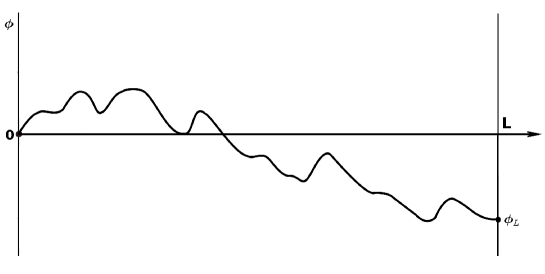
Figure 5: Continuous elastic string in a random potential, eq.(1.10)

First of all we can note that in the absence of the random potential in the Hamiltonian, eq.(1.10), the system describes simple thermal diffusion. Indeed, the probability that at time $\tau=L$ the trajectory arrives to the point $\phi(L)=\phi_{L}$ is given by the partition function

$$Z_{0}(\phi_{L})=\int_{\phi(0)=0}^{\phi(L)=\phi_{L}}{\cal D}[\phi(\tau)]\;\exp\biggl{\{}-\frac{1}{2T}\int_{0}^{L}d\tau\biggl{[}\frac{d\phi(\tau)}{d\tau}\biggr{]}^{2}\biggr{\}}$$ (1.13)

Simple Gaussian integration (with the proper choice of the integration measure of the functional integral) yields

$$Z_{0}(\phi_{L})=\frac{1}{\sqrt{2\pi TL}}\exp\biggl{\{}-\frac{\phi_{L}^{2}}{2TL}\biggr{\}}$$ (1.14)

In other words the typical deviation $<\phi_{L}>$ of the trajectory due to the thermal fluctuations growth as $\sqrt{T}\,L^{1/2}$ (and it shrinks to zero at $T=0$). On the other hand, in the presence of the random potential the two terms of the Hamiltonian (1.10) must balance each other. For a given value of the typical deviation $\phi_{L}$ the contribution of the elastic term can be estimated as $\phi_{L}^{2}/L$. Thus, if in the presence of disorder the free energy fluctuations of this system are scaling as $L^{1/3}$ (see e.g. hhf_85 ; numer1 ; numer2 ; kardar_87 ) we can conclude that the typical value of the trajectory deviations due to the action of the random potentials must grow as $\phi_{L}\sim L^{2/3}$ which is much faster than the pure thermal diffusion scaling $L^{1/2}$.

In what follows we are going to study the system defined by eqs.(1.10),(1.11) in all detail. It turns out that regardless of essential differences in the definition of this system and the previous models discussed above in sections 1.A-1.C, in the thermodynamic limit all these models becomes equivalent. The central result which will be proved in the next sections is in the following. In the limit $L\to\infty$ the free energy of the considered system can be represented as

$$F\;=\;f_{0}L\;+\;c\,L^{1/3}\;f$$ (1.15)

where $f_{0}$ is the linear free energy density, the constant $c=\frac{1}{2}(\beta^{2}u^{2})^{1/3}$, and the random quantity $f\sim 1$ (just like the quantity $s$ in eqs.(1.2)-(1.4)) is described by the universal TW distribution function (see section I.E)

I.4 Replica method

The replica method is widely used in the studies of systems containing quenched disorder (see e.g. ufn ; book ). For simplicity let us consider the string $\phi(\tau)$ with the zero boundary conditions: $\phi(0)=\phi(L)=0$. The partition function of a given sample described by the Hamiltonian, eq.(1.10), is

$$Z[V]=\int_{\phi(0)=0}^{\phi(L)=0}{\cal D}[\phi(\tau)]\;\mbox{\Large e}^{-\beta H[\phi,V]}$$ (1.16)

On the other hand, the partition function is related to the total free energy $F[V]$ via

$$Z[V]=\exp(-\beta F[V])$$ (1.17)

The free energy $F[V]$ is defined for a specific realization of the random potential $V$ and thus represent a random variable. Taking the $N$-th power of both sides of this relation and performing the averaging over the random potential $V$ we obtain

$$\overline{Z^{N}[V]}\equiv Z[N,L]=\overline{\exp(-\beta NF[V])}$$ (1.18)

where the quantity in the lhs of the above equation is called the replica partition function. Substituting here the free energy in the form $F=f_{0}L+c\,L^{1/3}\;f$, eq.(1.15), and redefining the partition function

$$Z[N,L]=\tilde{Z}[N,L]\;\mbox{\Large e}^{-\beta Nf_{0}L}$$ (1.19)

we get

$$\tilde{Z}[N,L]=\overline{\exp(-\lambda Nf)}$$ (1.20)

where $\lambda=\beta cL^{1/3}$. The averaging in the rhs of the above equation can be represented in terms of the distribution function $P_{L}(f)$ (which depends on the system size $L$). In this way we arrive to the following general relation between the replica partition function $\tilde{Z}[N,L]$ and the distribution function of the free energy fluctuations $P_{L}(f)$:

$$\tilde{Z}[N,L]\;=\;\int_{-\infty}^{+\infty}df\,P_{L}(f)\;\mbox{\Large e}^{-\lambda N\,f}$$ (1.21)

Of course, the most interesting object is the thermodynamic limit distribution function $P_{*}(f)=\lim_{L\to\infty}P_{L}(f)$ which is expected to be the universal quantity. The above equation is the bilateral Laplace transform of the function $P_{L}(f)$, and at least formally it allows to restore this function via inverse Laplace transform of the replica partition function $\tilde{Z}[N,L]$. In order to do so one has to compute $\tilde{Z}[N,L]$ for an arbitrary integer $N$ and then perform analytical continuation of this function from integer to arbitrary complex values of $N$. This is the standard strategy of the replica method in disordered systems where it is well known that very often the procedure of such analytic continuation turns out to be rather controversial point zirnbauer1 ; replicas . Even in rare cases when the derivation of the replica partition function $Z(N)=\overline{Z^{N}}$ can be done exactly, its further analytic continuation to non-integer $N$ appears to be ambiguous. The classical example of this situation is provided by the Derrida’s Random Energy Model in which the momenta $Z(N)$ growths as fast as $\exp(N^{2})$ at large $N$, and in this case there are many different distributions yielding the same values of $Z(N)$, but providing different values for the average free energy of the system REM . In our present system the situation is even worse because, as we will see later, the replica partition function growth here as $\exp(N^{3})$ at large $N$, and in this situation its analytic continuation from integer to non integer $N$ would be rather problematic point. It turns out, however, that in our present case it is possible to bypass the problem of the analytic continuation if instead of the distribution function $P_{*}(f)$ one would study its integral representation

$$W(x)\;=\;\int_{x}^{\infty}\;df\;P_{*}(f)$$ (1.22)

which gives the probability to find the fluctuation $f$ bigger that a given value $x$. Formally the function $W(x)$ can be defined as follows:

$$W(x) = \lim_{\lambda\to\infty}\sum_{N=0}^{\infty}\frac{(-1)^{N}}{N!}\exp(\lambda Nx)\;\overline{\tilde{Z}^{N}}$$

$$= \lim_{\lambda\to\infty}\sum_{N=0}^{\infty}\frac{(-1)^{N}}{N!}\;\overline{\exp(\lambda Nx-\lambda Nf)}$$

$$= \lim_{\lambda\to\infty}\overline{\exp\bigl{[}-\exp\bigl{(}\lambda(x-f)\bigr{)}\bigr{]}}\;=\;\overline{\theta(f-x)}$$

Thus, the probability function $W(x)$ can be computed in terms of the above replica partition function $\tilde{Z}[N,L]$ by summing over all replica integers

$$W(x)\;=\;\lim_{\lambda\to\infty}\sum_{N=0}^{\infty}\frac{(-1)^{N}}{N!}\exp(\lambda Nx)\;\tilde{Z}[N,L]$$ (1.24)

Of course, keeping in mind that $\tilde{Z}[N,L]\sim\exp(N^{3})$ at large $N$, we see that the above series is not that innocent. Here in accordance with the troubles conservation law instead of the problem of analytic continuation we are facing formally divergent series. Nevertheless, it can be shown that this sign alternating series can be regularized in the standard way (similarly to formally divergent sign alternating series $\sum_{k=0}^{\infty}(-1)^{k}a^{k}\;=\;(1+a)^{(-1)}$ which at $|a|>1$ is defined as the analytic continuation from the region $|a|<1$). This eventually allows to prove that the thermodynamic limit function $W(x)$, eq.(1.24), is defined by the universal Tracy-Widom distribution function.

I.5 Tracy-Widom distribution function

Originally the Tracy-Widom distribution function has been derived in the context of the statistical properties of the Gaussian Unitary Ensemble (GUE) of random Hermitian matrices Tracy-Widom . GUE is the set of $N\times N$ random complex Hermitian matrices $G_{ij}$ (such that $G_{ij}=G_{ji}^{*}$) whose elements are drawn independently from the Gaussian distribution

$${\cal P}[{\bf G}]\;=\;B_{N}\,\exp\Bigl{\{}-\frac{1}{2}Tr({\bf G}^{2})\Bigr{\}}$$ (1.25)

where $B_{N}$ is the normalization constant. The joint probability density of $N$ eigenvalues $\{\lambda_{1},\lambda_{2},...,\lambda_{N}\}$ of such matrices has rather compact form Wigner :

$${\cal P}[\lambda_{1},\lambda_{2},...,\lambda_{N}]\;=\;C_{N}\,\prod_{i\not=j}^{N}\Big{|}\lambda_{i}-\lambda_{j}\Big{|}^{2}\exp\Bigl{\{}-\sum_{i=1}^{N}\lambda_{i}^{2}\Bigr{\}}$$ (1.26)

where $C_{N}$ is the normalization constant. Using this joint probability density one can calculate various averaged characteristics of the eigenvalue statistics. For example, one can introduce the average density of the eigenvalues $\rho(\lambda,N)\;=\;\frac{1}{N}\sum_{i=1}^{N}\langle\delta(\lambda-\lambda_{i})\rangle$ where the averaging $\langle.....\rangle$ is performed with the probability distribution, eq.(1.26). Using the symmetry of this distribution one gets

$$\rho(\lambda,N)\;=\;\biggl{[}\prod_{i=2}^{N}\int_{-\infty}^{+\infty}\;d\lambda_{i}\biggr{]}{\cal P}[\lambda,\lambda_{2},...,\lambda_{N}]$$ (1.27)

It can be shown Wigner that in the limit of large $N$

$$\rho(\lambda,N)\;=\;\sqrt{\frac{2}{N\pi^{2}}\;\biggl{(}1-\frac{\lambda^{2}}{2N}\biggr{)}}$$ (1.28)

We see that on average the eigenvalues lie within the finite interval $\bigl{[}-\sqrt{2N}<\lambda<\sqrt{2N}\bigr{]}$ where, according to eq.(1.28), their density has the semi-circular form. This is one of the central results of the random matrix theory which is called the Wigner semi-circular law. In particular this result tells that on average the maximum eigenvalue $\lambda_{max}$ is equal to $\sqrt{2N}$. However, at large but finite $N$ the value of $\lambda_{max}$ is the random quantity which fluctuates from sample to sample. One may ask, what is the full probability distribution of the largest eigenvalue $\lambda_{max}$? This distribution can be computed in terms of the general probability density, eq.(1.26). Introducing standard notations of the random matrix theory we define the function $F_{2}(s)\equiv\mbox{Prob}\bigl{[}\lambda_{max}<s\bigr{]}$ which gives the probability that $\lambda_{max}$ is less than a given value $s$ (in these notations the functions $F_{1}(s)$, $F_{2}(s)$ and $F_{4}(s)$ denote the probability distributions of the largest eigenvalues in the Gaussian Orthogonal Ensemble (GOE), Gaussian Unitary Ensemble (GUE) and Gaussian Symplectic Ensemble (GSE) correspondingly Tracy-Widom2 ). By definition

$$F_{2}(s)\;=\;\biggl{[}\prod_{i=i}^{N}\int_{-\infty}^{s}\;d\lambda_{i}\biggr{]}{\cal P}[\lambda_{1},\lambda_{2},...,\lambda_{N}]\;\equiv\;\int_{-\infty}^{s}d\lambda\,P_{TW}(\lambda)$$ (1.29)

It is this problem which has been solved by Tracy and Widom in 1994 Tracy-Widom . It has been shown that at large $N$ the typical fluctuations of $\lambda_{max}$ around its mean value $\sqrt{2N}$ scale as $N^{-1/6}$, namely (c.f. eq.(1.2))

$$\lambda_{max}=\sqrt{2N}\;+\;\frac{1}{\sqrt{2}\,N^{1/6}}\,s$$ (1.30)

where the random quantity $s$ is described by $N$-independent distribution $P_{TW}(s)=dF_{2}(s)/ds$. The function $F_{2}(x)$, has the following explicit form

$$F_{2}(s)\;=\;\exp\biggl{(}-\int_{s}^{\infty}dt\;(t-s)\;q^{2}(t)\biggr{)}$$ (1.31)

or

$$P_{TW}(s)\;=\;\frac{d}{ds}F_{2}(s)\;=\;\exp\biggl{[}-\int_{s}^{\infty}dt\,(t-s)q^{2}(t)\biggr{]}\times\int_{s}^{\infty}dt\,q^{2}(t)$$ (1.32)

where the function $q(t)$ is the solution of the Panlevé II equation⁽¹⁾,

$$q^{\prime\prime}=tq+2q^{3}$$ (1.33)

with the boundary condition, $q(t\to+\infty)\sim Ai(t)$.

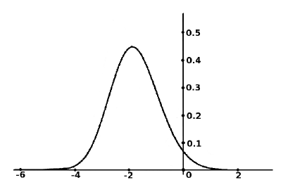
Figure 6: Tracy-Widom distribution function $P_{TW}(x)$, eq.(1.32).

The shape of the function $P_{TW}(s)$ is shown in Figure 6. Note that the asymptotic tails of this function are strongly asymmetric. While its right tail coincides the Airy function asymptotic $P_{TW}(s\to+\infty)\sim\exp\bigl{[}-\frac{4}{3}s^{3/2}\bigr{]}$, the left tail exhibits much faster decay $P_{TW}(s\to-\infty)\sim\exp\bigl{[}-\frac{1}{12}|s|^{3}\bigr{]}$

II Mapping to quantum bosons

Explicitly, the replica partition function, Eqs.(1.18), (1.16), of the system described by the Hamiltonian, Eq.(1.10), is

$$Z(N,L)=\prod_{a=1}^{N}\int_{\phi_{a}(0)=0}^{\phi_{a}(L)=0}{\cal D}\phi_{a}(\tau)\;\overline{\exp\Biggl{[}-\beta\int_{0}^{L}d\tau\sum_{a=1}^{N}\bigl{\{}\frac{1}{2}\bigl{[}\partial_{\tau}\phi_{a}(\tau)\bigr{]}^{2}+V[\phi_{a}(\tau),\tau]\bigr{\}}\Biggr{]}}$$ (2.1)

Since the random potential $V[\phi,\tau]$ has the Gaussian distribution the disorder averaging $\overline{(...)}$ in the above equation is very simple:

$$\overline{\exp\Biggl{[}-\beta\int_{0}^{L}d\tau\sum_{a=1}^{N}V[\phi_{a}(\tau),\tau]\Biggr{]}}\;=\;\exp\Biggl{[}\frac{\beta^{2}}{2}\int\int_{0}^{L}d\tau d\tau^{\prime}\sum_{a,b=1}^{N}\overline{V[\phi_{a}(\tau),\tau]V[\phi_{b}(\tau^{\prime}),\tau^{\prime}]}\Biggr{]}$$ (2.2)

Using Eq.(1.11) we find:

$$Z(N,L)=\prod_{a=1}^{N}\int_{\phi_{a}(0)=0}^{\phi_{a}(L)=0}{\cal D}\phi_{a}(\tau)\;\exp\Biggl{[}-\frac{1}{2}\beta\int_{0}^{L}d\tau\Bigl{\{}\sum_{a=1}^{N}\bigl{[}\partial_{\tau}\phi_{a}(\tau)\bigr{]}^{2}-\beta u\sum_{a,b=1}^{N}\delta\bigl{[}\phi_{a}(\tau)-\phi_{b}(\tau)\bigr{]}\Bigr{\}}\Biggr{]}$$ (2.3)

It should be noted that the second term in the exponential of the above equation contain formally divergent contributions proportional to $\delta(0)$ (due to the terms with $a=b$). In fact, this is just an indication that the continuous model, Eqs.(1.10)-(1.11) is ill defined as short distances and requires proper lattice regularization. Of course, the corresponding lattice model Eqs.(1.6)-(1.7) contains no divergences, and the terms with $a=b$ in the exponential of the corresponding replica partition function would produce irrelevant constant $\frac{1}{2}L\beta^{2}uN\delta(0)$ (where the lattice version of $\delta(0)$ has a finite value). Since the lattice regularization has no impact on the continuous long distance properties of the considered system this term will be just omitted in our further study.

Introducing the $N$-component scalar field replica Hamiltonian

$$H_{N}[{\boldsymbol{\phi}}]=\frac{1}{2}\int_{0}^{L}d\tau\Biggl{(}\sum_{a=1}^{N}\bigl{[}\partial_{\tau}\phi_{a}(\tau)\bigr{]}^{2}-\beta u\sum_{a\not=b}^{N}\delta\bigl{[}\phi_{a}(\tau)-\phi_{b}(\tau)\bigr{]}\Biggr{)}$$ (2.4)

for the replica partition function, Eq.(2.3), we obtain the standard expression

$$Z(N,L)=\prod_{a=1}^{N}\int_{\phi_{a}(0)=0}^{\phi_{a}(L)=0}{\cal D}\phi_{a}(\tau)\;\mbox{\Large e}^{-\beta H_{N}[{\boldsymbol{\phi}}]}$$ (2.5)

where ${\boldsymbol{\phi}}\equiv\{\phi_{1},\dots,\phi_{N}\}$. According to the above definition this partition function describes the statistics of $N$ $\delta$-interacting (attracting) trajectories $\phi_{a}(\tau)$ all starting (at $\tau=0$) and ending (at $\tau=L$) at zero: $\phi_{a}(0)=\phi_{a}(L)=0$

In order to map the problem to one-dimensional quantum bosons, instead of the above replica partition function, eq.(2.5), let us introduce more general object

$$\Psi({\bf x};t)=\prod_{a=1}^{N}\int_{\phi_{a}(0)=0}^{\phi_{a}(t)=x_{a}}{\cal D}\phi_{a}(\tau)\;\mbox{\Large e}^{-\beta H_{N}[{\boldsymbol{\phi}}]}$$ (2.6)

which describes $N$ trajectories $\phi_{a}(\tau)$ all starting at zero ($\phi_{a}(0)=0$), but ending at $\tau=t$ in arbitrary given points $\{x_{1},...,x_{N}\}$. One can easily show that instead of using the path integral, $\Psi({\bf x};t)$ may be obtained as the solution of the linear differential equation

$$\partial_{t}\Psi({\bf x};t)\;=\;\frac{1}{2\beta}\sum_{a=1}^{N}\partial_{x_{a}}^{2}\Psi({\bf x};t)\;+\;\frac{1}{2}\beta^{2}u\sum_{a\not=b}^{N}\delta(x_{a}-x_{b})\Psi({\bf x};t)$$ (2.7)

with the initial condition

$$\Psi({\bf x};0)=\Pi_{a=1}^{N}\delta(x_{a})$$ (2.8)

One can easily see that Eq.(2.7) is the imaginary-time Schrödinger equation

$$-\partial_{t}\Psi({\bf x};t)=\hat{H}\Psi({\bf x};t)$$ (2.9)

with the Hamiltonian

$$\hat{H}=-\frac{1}{2\beta}\sum_{a=1}^{N}\partial_{x_{a}}^{2}-\frac{1}{2}\beta^{2}u\sum_{a\not=b}^{N}\delta(x_{a}-x_{b})$$ (2.10)

which describes $N$ bose-particles of mass $\beta$ interacting via the attractive two-body potential $-\beta^{2}u\delta(x)$. The original replica partition function, Eq.(2.5), then is obtained via a particular choice of the final-point coordinates,

$$Z(N,L)=\Psi({\bf 0};L).$$ (2.11)

Historically the main interest in the studies of such type of systems was devoted to the quantum bosons with repulsion. It is for the case of repulsive interactions the free energy of the $N$ particle system reveals ”correct” extensive behavior, $F\propto N$. The eigenfunction of $N$-particle Hamiltonian Eq.(2.10), with repulsive interactions, $u<0$, have been derived by Lieb and Liniger in 1963 Lieb-Liniger (for details see Appendix A, as well as Refs. bogolubov ; gaudin ). The system of attractive bosons remained much less studied. The free energy of such system reveals ”bad” thermodynamic limit behavior, namely $F\propto-N^{3}$. Besides, as will be shown later, the structure of the eigenstates of such system is much more complicated compared to the case of repulsion. The spectrum and some properties of the eigenfunctions for attractive ($u>0$) one-dimensional quantum boson system have been derived by McGuire McGuire and by Yang Yang (see also Ref. Takahashi ; Calabrese ). Detailed structure and the properties of these wave functions are described in Appendix B.

A generic eigenstate of such system consists of $M$ ($1\leq M\leq N$) ”clusters” $\{\Omega_{\alpha}\}$ $(\alpha=1,...,M)$ of bound particles. Each cluster is characterized by the momentum $q_{\alpha}$ of its center of mass motion, and by the number $n_{\alpha}$ of particles contained in it (such that $\sum_{\alpha=1}^{M}n_{\alpha}=N$). Correspondingly, the eigenfunction $\Psi_{\bf q,n}^{(M)}(x_{1},...,x_{N})$ of such state is characterized by $M$ continuous parameters ${\bf q}=(q_{1},...,q_{M})$ and $M$ integer parameters ${\bf n}=(n_{1},...,n_{M})$ (see Appendix B2, Eq.(B.27)). The energy spectrum of this state is

$$E_{M}({\bf q,n})=\frac{1}{2\beta}\sum_{\alpha=1}^{M}\;n_{\alpha}q_{\alpha}^{2}-\frac{\kappa^{2}}{24\beta}\sum_{\alpha=1}^{M}(n_{\alpha}^{3}-n_{\alpha})$$ (2.12)

where

$$\kappa\;=\;\beta^{3}u$$ (2.13)

A general time dependent solution $\Psi({\bf x},t)$ of the Schrödinger equation (2.7) with the initial conditions, Eq.(2.8), can be represented in the form of the linear combination of the eigenfunctions $\Psi_{\bf q,n}^{(M)}({\bf x})$ (Appendix B4, Eq.(B.50)):

$$\Psi({\bf x},t)\;=\;\sum_{M=1}^{N}\;{\sum_{{\bf n}}}^{\prime}\;\int^{\prime}{\cal D}{\bf q}\;\;\Psi_{\bf q,n}^{(M)}({\bf x})\Psi_{\bf q,n}^{(M)^{*}}({\bf 0})\;\exp\bigl{[}-E_{M}({\bf q,n})\;t\bigr{]}$$ (2.14)

where the summations over the integer parameters $n_{\alpha}$ and the integrations over the momenta $q_{\alpha}$ are performed in a restricted subspace, Eqs.(B.42)-(B.45) and (B.51), which reflects the specific symmetry properties of the eigenfunctions $\Psi_{\bf q,n}^{(M)}({\bf x})$. Correspondingly, according to Eq.(2.11), for the replica partition function of the original directed polymer problem one gets (Appendix B4, Eq.(B.59))

$$Z(N,L)\;=\;\sum_{M=1}^{N}\;\frac{1}{M!}\biggl{[}\prod_{\alpha=1}^{M}\int_{-\infty}^{+\infty}\;\frac{dq_{\alpha}}{2\pi}\sum_{n_{\alpha}=1}^{\infty}\biggr{]}\;{\boldsymbol{\delta}}\biggl{(}\sum_{\alpha=1}^{M}n_{\alpha},\;N\biggr{)}\;\big{|}\Psi_{\bf q,n}^{(M)}({\bf 0})\big{|}^{2}\;\mbox{\LARGE e}^{-E_{M}({\bf q,n})L}$$ (2.15)

where due to the symmetry of the function $f\bigl{(}{\bf q},{\bf n}\bigr{)}=\bigl{|}\Psi_{\bf q,n}^{(M)}({\bf 0})\bigr{|}^{2}\;\exp\bigl{[}-E_{M}({\bf q,n})\;L\bigr{]}$ with respect to permutations of all its $M$ pairs of arguments $(q_{\alpha},n_{\alpha})$ the integrations over $M$ momenta $q_{\alpha}$ can be extended to the whole space $R_{M}$ while the summations over $n_{\alpha}$’s are bounded by the only constrain $\sum_{\alpha=1}^{M}n_{\alpha}=N$ (for simplicity, due to the presence of the Kronecker symbol ${\boldsymbol{\delta}}\bigl{(}\sum_{\alpha}n_{\alpha},\;N\bigr{)}$, the summations over $n_{\alpha}$’s are extended to infinity).

III Solution of the one-dimensional directed polymers problem

Using the explicit form of the wave functions $\Psi_{\bf q,n}^{(M)}({\bf x})$, Eq.(B.27), the expression in Eq.(2.15) for the replica partition function can be reduced to (Appendix B4, Eq.(B.61)-(B.62))

$$Z(N,L)\;=\mbox{\LARGE e}^{-\beta NLf_{0}}\;\;\tilde{Z}(N,\lambda)$$ (3.1)

where $f_{0}=\frac{1}{24}\beta^{4}u^{2}-\frac{1}{\beta L}\ln(\beta^{3}u)$ is the linear (selfaveraging) free energy density (cf. Eq.(1.19)), and

$$\tilde{Z}(N.L) = N!\;\int_{-\infty}^{+\infty}\frac{dq}{2\pi\kappa N}\;\exp\Bigl{[}-\frac{L}{2\beta}Nq^{2}+\frac{\kappa^{2}L}{24\beta}N^{3}\Bigr{]}\;+$$ (3.2)

$$+ N!\;\sum_{M=2}^{N}\frac{1}{M!}\biggl{[}\prod_{\alpha=1}^{M}\sum_{n_{\alpha}=1}^{\infty}\int_{-\infty}^{+\infty}\frac{dq_{\alpha}}{2\pi\kappa n_{\alpha}}\biggr{]}\;{\boldsymbol{\delta}}\biggl{(}\sum_{\alpha=1}^{M}n_{\alpha},\;N\biggr{)}\prod_{\alpha<\beta}^{M}\frac{\big{|}q_{\alpha}-q_{\beta}-\frac{i\kappa}{2}(n_{\alpha}-n_{\beta})\big{|}^{2}}{\big{|}q_{\alpha}-q_{\beta}-\frac{i\kappa}{2}(n_{\alpha}+n_{\beta})\big{|}^{2}}\times$$

$$\times \exp\Bigl{[}-\frac{L}{2\beta}\sum_{\alpha=1}^{M}n_{\alpha}q_{\alpha}^{2}+\frac{\kappa^{2}L}{24\beta}\sum_{\alpha=1}^{M}n_{\alpha}^{3}\Bigr{]}$$

The first term in the above expression is the contribution of the ground state $(M=1)$, while the next terms $(M\geq 2)$ are the contributions of the rest of the energy spectrum.

The terms cubic in $n_{\alpha}$ in the exponential of Eq. (3.2) can be linearised with the help of Airy function, using the standard relation (see Appendix C)

$$\exp\Bigl{(}\frac{1}{3}\lambda^{3}n^{3}\Bigr{)}\;=\;\int_{-\infty}^{+\infty}dy\;\operatorname{Ai}(y)\;\exp(\lambda n)$$ (3.3)

Redefining the momenta, $q_{\alpha}=\bigl{(}\beta\kappa/L\bigr{)}^{1/3}p_{\alpha}$ and introducing a new parameter

$$\lambda(L)\;=\;\frac{1}{2}\biggl{(}\frac{L}{\beta}\kappa^{2}\biggr{)}^{1/3}\;=\;\frac{1}{2}\Bigl{(}\beta^{5}u^{2}L\Bigr{)}^{1/3}$$ (3.4)

we get

$$\tilde{Z}(N,\lambda) = N!\int\int_{-\infty}^{+\infty}\frac{dydp}{4\pi\lambda N}\;\operatorname{Ai}(y)\;\mbox{\LARGE e}^{\lambda N(y-p^{2})}+$$

$$+ N!\sum_{M=2}^{N}\frac{1}{M!}\biggl{[}\prod_{\alpha=1}^{M}\sum_{n_{\alpha}=1}^{\infty}\int\int_{-\infty}^{+\infty}\frac{dy_{\alpha}dp_{\alpha}}{4\pi\lambda n_{\alpha}}\operatorname{Ai}(y_{\alpha})\;\mbox{\LARGE e}^{\lambda n_{\alpha}(y_{\alpha}-p^{2}_{\alpha})}\biggr{]}\prod_{\alpha<\beta}^{M}\frac{\big{|}\lambda(n_{\alpha}-n_{\beta})-i(p_{\alpha}-p_{\beta})\big{|}^{2}}{\big{|}\lambda(n_{\alpha}+n_{\beta})-i(p_{\alpha}-p_{\beta})\big{|}^{2}}\;{\boldsymbol{\delta}}\biggl{(}\sum_{\alpha=1}^{M}n_{\alpha},\;N\biggr{)}$$

After shifting the Airy function parameters of integration $y_{\alpha}\to y_{\alpha}+p_{\alpha}^{2}$ the expression for $\tilde{Z}(N,\lambda)$ becomes sufficiently compact:

$$\tilde{Z}(N,\lambda) = N!\int\int_{-\infty}^{+\infty}\frac{dydp}{4\pi\lambda N}\;\operatorname{Ai}(y+p^{2})\;\mbox{\LARGE e}^{\lambda Ny}+$$

$$+ N!\sum_{M=2}^{N}\frac{1}{M!}\biggl{[}\prod_{\alpha=1}^{M}\sum_{n_{\alpha}=1}^{\infty}\int\int_{-\infty}^{+\infty}\frac{dy_{\alpha}dp_{\alpha}}{4\pi\lambda n_{\alpha}}\operatorname{Ai}(y_{\alpha}+p^{2}_{\alpha})\;\mbox{\LARGE e}^{\lambda n_{\alpha}y_{\alpha}}\biggr{]}\prod_{\alpha<\beta}^{M}\frac{\big{|}\lambda(n_{\alpha}-n_{\beta})-i(p_{\alpha}-p_{\beta})\big{|}^{2}}{\big{|}\lambda(n_{\alpha}+n_{\beta})-i(p_{\alpha}-p_{\beta})\big{|}^{2}}\;{\boldsymbol{\delta}}\biggl{(}\sum_{\alpha=1}^{M}n_{\alpha},\;N\biggr{)}$$

Now, using the Cauchy double alternant identity

$$\frac{\prod_{\alpha<\beta}^{M}(a_{\alpha}-a_{\beta})(b_{\alpha}-b_{\beta})}{\prod_{\alpha,\beta=1}^{M}(a_{\alpha}-b_{\beta})}\;=\;(-1)^{M(M-1)/2}\det\Bigl{[}\frac{1}{a_{\alpha}-b_{\beta}}\Bigr{]}_{\alpha,\beta=1,...M}$$ (3.7)

and introducing $a_{\alpha}=p_{\alpha}-i\lambda n_{\alpha}$ and $b_{\alpha}=p_{\alpha}+i\lambda n_{\alpha}$, the product term in eq.(III) can be represented in the determinant form:

$$\prod_{\alpha<\beta}^{M}\frac{\big{|}\lambda(n_{\alpha}-n_{\beta})-i(p_{\alpha}-p_{\beta})\big{|}^{2}}{\big{|}\lambda(n_{\alpha}+n_{\beta})-i(p_{\alpha}-p_{\beta})\big{|}^{2}}=\biggl{[}\prod_{\alpha=1}^{M}(2\lambda n_{\alpha})\biggr{]}\;\det\Bigl{[}\frac{1}{\lambda n_{\alpha}-ip_{\alpha}+\lambda n_{\beta}+ip_{\beta}}\Bigr{]}_{\alpha,\beta=1,...M}$$ (3.8)

Substituting now the expression for the replica partition function $\tilde{Z}(N,\lambda)$ into the definition of the probability function, eq.(1.24), we can perform summation over $N$ (which would lift the constraint $\sum_{\alpha=1}^{M}n_{\alpha}=N$) and obtain:

$$W(x)=\lim_{\lambda\to\infty}\Biggl{\{}1+\sum_{M=1}^{\infty}\frac{(-1)^{M}}{M!}\Biggl{[}\prod_{\alpha=1}^{M}\int\int_{-\infty}^{+\infty}\frac{dy_{\alpha}dp_{\alpha}}{2\pi}\operatorname{Ai}(y_{\alpha}+p^{2}_{\alpha})\sum_{n_{\alpha}=1}^{\infty}(-1)^{n_{\alpha}-1}\mbox{\LARGE e}^{\lambda n_{\alpha}(y_{\alpha}+x)}\Biggr{]}\det\Bigl{[}\frac{1}{\lambda n_{\alpha}-ip_{\alpha}+\lambda n_{\beta}+ip_{\beta}}\Bigr{]}\Biggr{\}}$$ (3.9)

The above expression in nothing else but the expansion of the Fredholm determinant $\det(1-\hat{K})$ (see e.g. Mehta , Appendix D) with the kernel

$$\hat{K}\equiv K\bigl{[}(n,p);(n^{\prime},p^{\prime})\bigr{]}=\Biggl{[}\int_{-\infty}^{+\infty}dy\operatorname{Ai}(y+p^{2})(-1)^{n-1}\mbox{\LARGE e}^{\lambda n(y+x)}\Biggr{]}\frac{1}{\lambda n-ip+\lambda n^{\prime}+ip^{\prime}}$$ (3.10)

Using the exponential representation of this determinant we get

$$W(x)=\lim_{\lambda\to\infty}\exp\Bigl{[}-\sum_{M=1}^{\infty}\frac{1}{M}\;\mbox{Tr}\hat{K}^{M}\Bigr{]}$$ (3.11)

where

$$\mbox{Tr}\hat{K}^{M} = \Biggl{[}\prod_{\alpha=1}^{M}\int\int_{-\infty}^{+\infty}\frac{dy_{\alpha}dp_{\alpha}}{2\pi}\operatorname{Ai}(y_{\alpha}+p^{2}_{\alpha})\sum_{n_{\alpha}=1}^{\infty}(-1)^{n_{\alpha}-1}\mbox{\LARGE e}^{\lambda n_{\alpha}(y_{\alpha}+x)}\Biggr{]}\times$$ (3.12)

$$\times \frac{1}{(\lambda n_{1}-ip_{1}+\lambda n_{2}+ip_{2})(\lambda n_{2}-ip_{2}+\lambda n_{3}+ip_{3})...(\lambda n_{M}-ip_{M}+\lambda n_{1}+ip_{1})}$$

Substituting here

$$\frac{1}{\lambda n_{\alpha}-ip_{\alpha}+\lambda n_{\alpha+1}+ip_{\alpha+1}}=\int_{0}^{\infty}d\omega_{\alpha}\exp\bigl{[}-(\lambda n_{\alpha}-ip_{\alpha}+\lambda n_{\alpha+1}+ip_{\alpha+1})\omega_{\alpha}\bigr{]}$$ (3.13)

one can easily perform the summation over $n_{\alpha}$’s. Taking into account that

$$\lim_{\lambda\to\infty}\sum_{n=1}^{\infty}(-1)^{n-1}\mbox{\LARGE e}^{\lambda nz}\;=\;\lim_{\lambda\to\infty}\frac{\mbox{\LARGE e}^{\lambda z}}{1+\mbox{\LARGE e}^{\lambda z}}=\theta(z)$$ (3.14)

we get

$$\lim_{\lambda\to\infty}Tr\;\hat{K}^{M}=\prod_{\alpha=1}^{M}\int\int_{-\infty}^{+\infty}\frac{dy_{\alpha}dp_{\alpha}}{2\pi}\int_{0}^{\infty}d\omega_{\alpha}\operatorname{Ai}(y_{\alpha}+p^{2}_{\alpha})\theta(y_{\alpha}+x-\omega_{\alpha}-\omega_{\alpha-1})\mbox{\LARGE e}^{ip_{\alpha}(\omega_{\alpha}-\omega_{\alpha-1})}$$ (3.15)

where by definition $\omega_{0}\equiv\omega_{M}$. Shifting the integration parameters, $y_{\alpha}\to y_{\alpha}-x+\omega_{\alpha}+\omega_{\alpha-1}$ and $\omega_{\alpha}\to\omega_{\alpha}+x/2$, we obtain

$$\lim_{\lambda\to\infty}Tr\;\hat{K}^{M}=\prod_{\alpha=1}^{M}\int_{0}^{\infty}dy_{\alpha}\int_{-\infty}^{+\infty}\frac{dp_{\alpha}}{2\pi}\int_{-x/2}^{\infty}d\omega_{\alpha}\operatorname{Ai}(y_{\alpha}+p^{2}_{\alpha}+\omega_{\alpha}+\omega_{\alpha-1})\;\mbox{\LARGE e}^{ip_{\alpha}(\omega_{\alpha}-\omega_{\alpha-1})}$$ (3.16)

Using the Airy function integral representation, and taking into account that it satisfies the differential equation, $\operatorname{Ai}^{\prime\prime}(t)=t\operatorname{Ai}(t)$, one can easily perform the following integrations (see Appendix C):

$$\int_{0}^{\infty}dy\int_{-\infty}^{+\infty}\frac{dp}{2\pi}\operatorname{Ai}(y+p^{2}+\omega+\omega^{\prime})\mbox{\LARGE e}^{ip(\omega-\omega^{\prime})} = 2^{-1/3}\int_{0}^{\infty}dy\operatorname{Ai}\bigl{(}2^{1/3}\omega+y\bigr{)}\operatorname{Ai}\bigl{(}2^{1/3}\omega^{\prime}+y\bigr{)}$$

$$= \frac{\operatorname{Ai}\bigl{(}2^{1/3}\omega\bigr{)}\operatorname{Ai}^{\prime}\bigl{(}2^{1/3}\omega^{\prime}\bigr{)}-\operatorname{Ai}^{\prime}\bigl{(}2^{1/3}\omega\bigr{)}\operatorname{Ai}\bigl{(}2^{1/3}\omega^{\prime}\bigr{)}}{\omega-\omega^{\prime}}$$

Redefining $\omega_{\alpha}\to\omega_{\alpha}2^{-1/3}$ we find

$$\lim_{\lambda\to\infty}Tr\hat{K}^{M}=\int\int...\int_{-x/2^{2/3}}^{\infty}d\omega_{1}d\omega_{2}...d\omega_{M}K_{A}(\omega_{1},\omega_{2})K_{A}(\omega_{2},\omega_{3})...K_{A}(\omega_{M},\omega_{1})$$ (3.18)

where

$$K_{A}(\omega,\omega^{\prime})\;=\;\frac{\operatorname{Ai}(\omega)\operatorname{Ai}^{\prime}(\omega^{\prime})-\operatorname{Ai}^{\prime}(\omega)\operatorname{Ai}(\omega^{\prime})}{\omega-\omega^{\prime}}$$ (3.19)

is the so called Airy kernel. This proves that in the thermodynamic limit, $L\to\infty$, the probability function $W(x)$, eq.(1.22), is defined by the Fredholm determinant,

$$W(x)\;=\;\det[1-\hat{K}_{A}]\equiv F_{2}(-x/2^{2/3})$$ (3.20)

where $\hat{K}_{A}$ is the integral operator on $[-x/2^{2/3},\infty)$ with the Airy kernel, eq.(3.19). This is the Tracy-Widom distribution function which has the following explicit form (see Appendix D):

$$F_{2}(s)\;=\;\exp\Bigl{(}-\int_{s}^{\infty}dt\;(t-s)\;q^{2}(t)\Bigr{)}$$ (3.21)

where the function $q(t)$ is the solution of the Panlevé II equation, $q^{\prime\prime}=tq+2q^{3}$ with the boundary condition, $q(t\to+\infty)\sim Ai(t)$. Note that according to Eqs.(1.22), (1.32) and (3.20), $P_{*}(x)=2^{-2/3}P_{TW}(-2^{-2/3}x)$

IV Conclusions

The first breakthrough in the studies of one-dimensional directed polymers in random potential was due to the work of Kardar kardar_87 , in which the problem has been reduced to $N$-particle system of quantum bosons with attractive interactions. By that time the very first idea was that in the thermodynamic limit it would be sufficient to take into account only the contribution of the ground state whose energy was well known. Indeed, for any integer $N>1$ the contribution of the excited states in the limit $L\to\infty$ are exponentially small compared to that of the ground state. In the framework of this approach it has been demonstrated that the free energy fluctuations grow as $L^{1/3}$ while the typical value of the polymers deviations scale as $L^{2/3}$ which, in particular, was in perfect agreement with numerical studies.

However, more detailed investigations demonstrated that the above approach reveals serious pathologies. In particular it turned out that the second cummulant of the free energy $\bigl{(}\overline{F^{2}}-\overline{F}^{2}\bigr{)}$ appears to be identically equal to zero! This is possible only in two cases: either the quantity $F$ is not random (which contradicts to the fact that its fluctuations scale as $L^{1/3}$), or the distribution function of the this quantity is not positively defined (which, of course, makes no physical sense). Simple mathematical analysis demonstrated that the origin of this pathology is hidden in the replicas ”magic operations”: on one hand, all the calculations are performed assuming that the replica parameter $N$ (number of particles) is an integer $N>1$, while on the other hand, in the thermodynamic limit $L\to\infty$ the relevant values of the parameter $N$ which defines the physical properties of the original random system appears to be in the region $N\to 0$. In other words, the replica method assumes analytic continuation of the result obtained for arbitrary integers $N$ to the region $N\to 0$. The problem is that, first, such analytic continuation is not always unambiguous (see e.g. REM ; replicas ), and second, any approximations in the calculations of the integer-valued replica partition function are quite risky for the validity of the further analytic continuation to non-integer values of $N$.

For the problem under consideration the point is that, in fact, neglected exponentially small contributions at integers $N>1$ appear to be quite essential in the region $N\to 0$, which defines the properties of the free energy distribution function $P_{*}(f)=\lim_{L\to\infty}P_{L}(f)$. In other words, the problem is that the two limits, $L\to\infty$ and $N\to 0$, do not commute Medina_93 ; dirpoly .

Nevertheless, in terms of this approximation (assuming the universal scaling $L^{1/3}$ of the free energy fluctuations) one can derive the left tail of the distribution function $P_{*}(f)$ which is given by the asymptotics of the Airy function, $P_{*}(f\to-\infty)\sim\exp\bigl{(}-\frac{2}{3}\big{|}f\big{|}^{3/2}\bigr{)}$ Zhang . For the first time the form of the right tail of this distribution function, $P_{*}(f\to+\infty)\sim\exp\bigl{[}-(const)f^{3}\bigr{]}$, has been derived in terms of the optimal fluctuation approach KK1 ; KK2 ; KK3 , where it has been demonstrated that both asymptotics (left and right) of the function $P_{*}(f)$ are consistent with the Tracy-Widom distribution Tracy-Widom which was known to describe the statistical properties of many other systems PNG_Spohn ; LIS ; LCS ; oriented_boiling ; ballistic_decomposition ; DP_johansson .

For the first time TW distribution for the directed polymers with $\delta$-correlated random potentials was derived in terms of the distribution of the solutions of the KPZ equation KPZ-TW1 ; KPZ-TW2 , which, in particular, describes the domain walls growth, and which is equivalent to the present system. Almost simultaneously the exact solution of the one-dimensional directed polymer problem has been found in terms of of the replica method, which involved the summation over the whole spectrum of excited states in the corresponding $N$-particle quantum boson system Dotsenko1 ; Dotsenko2 ; Dotsenko3 ; LeDoussal . These calculations resulted in the derivation of the entire free energy distribution, which was proved to coincide with TW distribution function.

The Tracy-Widom function, Eq.(3.21), was originally derived for rather specific mathematical problem, namely for the probability distribution of the largest eigenvalue of a $N\times N$ random hermitian matrix in the limit $N\to\infty$ Tracy-Widom . It is amazing but now there are exists a long list of statistical systems (which at first sight have just nothing to do with the original random matrix problem) whose macroscopic properties are described by the same universal TW distribution function. In other words, all the above observations indicate there exist a kind of ”superuniversality” for the entire class of various random systems.

In this review we have described the exact solution of the problem which remained unsolved during last almost thirty years. It should be stressed that this solution has been obtained in terms of the replica method. This is very rare case when the solution of a non-trivial problem has been found without using heuristic ”replica magic” operations, quite typical for this method, which usually forced to think that the ”replica method” and the ”exact solution” are two things absolutely incompatible. Hopefully finding exact solution is not always means the end of the story: methodology and created mathematical technique could be used for solving numerous other problems still waiting for their solutions…

Appendix A

Quantum bosons with repulsive interactions

1. Eigenfunctions

The eigenstates equation for $N$-particle system of one-dimensional quantum bosons with $\delta$-interactions is

$$\frac{1}{2}\sum_{a=1}^{N}\partial_{x_{a}}^{2}\Psi({\bf x})\;+\;\frac{1}{2}\kappa\sum_{a\not=b}^{N}\delta(x_{a}-x_{b})\Psi({\bf x})\;=\;-\beta E\Psi({\bf x})$$ (A.1)

(where $\kappa=\beta^{3}u$). Due to the symmetry of the wave function with respect to permutations of its arguments it is sufficient to consider it in the sector

$$x_{1}\;<\;x_{2}\;<\;...\;<\;x_{N}$$ (A.2)

as well as at its boundary. Inside this sector the wave function $\Psi({\bf x})$ satisfy the equation

$$\frac{1}{2}\sum_{a=1}^{N}\partial_{x_{a}}^{2}\Psi({\bf x})\;=\;-\beta E\Psi({\bf x})$$ (A.3)

which describes $N$ free particles, and its generic solution is the linear combination of $N$ plane waves characterized by $N$ momenta $\{q_{1},q_{2},...,q_{N}\}\equiv{\bf q}$. Integrating Eq.(A.1) over the variable $(x_{i+1}-x_{i})$ in a small interval around zero, $|x_{i+1}-x_{i}|<\epsilon\to 0$, and assuming that the other variables $\{x_{j}\}$ (with $j\not=i,i+1$) belong to the sector, Eq.(A.2), one easily finds that the wave function $\Psi({\bf x})$ must satisfy the following boundary conditions:

$$\bigl{(}\partial_{x_{i+1}}-\partial_{x_{i}}+\kappa\bigr{)}\Psi({\bf x})\bigg{|}_{x_{i+1}=x_{i}+0}\;=\;0$$ (A.4)

Functions satisfying both Eq. (A.3) and the boundary conditions Eq. (A.4) can be written in the form

$$\Psi_{q_{1}...q_{N}}(x_{1},...,x_{N})\equiv\Psi^{(N)}_{\bf q}({\bf x})\;=\;C\biggl{(}\prod_{a<b}^{N}\bigl{[}\partial_{x_{a}}-\partial_{x_{b}}+\kappa\bigr{]}\biggr{)}\;\det\Bigl{[}\exp(iq_{c}\,x_{d})\Bigr{]}_{(c,d)=1,...,N}$$ (A.5)

where $C$ is the normalization constant to be defined later. First of all, it is evident that being the linear combination of the plane waves, the above wave function satisfy Eq.(A.3). To demonstrate which way this function satisfy the boundary conditions, Eq.(A.4), let us check it for the case $i=1$. According to Eq.(A.5), the wave function $\Psi^{(N)}_{\bf q}({\bf x})$ can be represented in the form

$$\Psi^{(N)}_{\bf q}({\bf x})\;=\;-\bigl{(}\partial_{x_{2}}-\partial_{x_{1}}-\kappa\bigr{)}\tilde{\Psi}^{(N)}_{\bf q}({\bf x})$$ (A.6)

where

$$\tilde{\Psi}^{(N)}_{\bf q}({\bf x})\;=\;C\biggl{(}\prod_{a=3}^{N}\bigl{[}\partial_{x_{1}}-\partial_{x_{a}}+\kappa\bigr{]}\bigl{[}\partial_{x_{2}}-\partial_{x_{a}}+\kappa\bigr{]}\biggr{)}\biggl{(}\prod_{3\leq a<b}^{N}\bigl{[}\partial_{x_{a}}-\partial_{x_{b}}+\kappa\bigr{]}\biggr{)}\det\Bigl{[}\exp(iq_{c}\,x_{d})\Bigr{]}_{(c,d)=1,...,N}$$ (A.7)

One can easily see that this function is antisymmetric with respect to the permutation of $x_{1}$ and $x_{2}$. Substituting Eq.(A.6) into Eq.(A.4) (with $i=1$) we get

$$-\biggl{[}\bigl{(}\partial_{x_{2}}-\partial_{x_{1}}\bigr{)}^{2}-\kappa^{2}\biggr{]}\tilde{\Psi}^{(N)}_{\bf q}({\bf x})\bigg{|}_{x_{2}=x_{1}}\;=\;0$$ (A.8)

Given the antisymmetry of the l.h.s expression with respect to the permutation of $x_{1}$ and $x_{2}$ the above condition is indeed satisfied at boundary $x_{1}=x_{2}$.

Since the eigenfunction $\Psi^{(N)}_{\bf q}({\bf x})$ satisfying Eq.(A.1) must be symmetric with respect to permutations of its arguments, the function, Eq.(A.5), can be easily continued beyond the sector, Eq.(A.2), to the entire space of variables $\{x_{1},x_{2},...,x_{N}\}\in R_{N}$,

$$\Psi^{(N)}_{\bf q}({\bf x})\;=\;C\biggl{(}\prod_{a<b}^{N}\Bigl{[}-i\bigl{(}\partial_{x_{a}}-\partial_{x_{b}}\bigr{)}+i\kappa\operatorname{sgn}(x_{a}-x_{b})\Bigr{]}\biggr{)}\;\det\Bigl{[}\exp(iq_{c}\,x_{d})\Bigr{]}_{(c,d)=1,...,N}$$ (A.9)

where, by definition, the differential operators $\partial_{x_{a}}$ act only on the exponential terms and not on the $\operatorname{sgn}(x)$ functions, and for further convenience we have redefined $i^{N(N-1)/2}C\to C$. Explicitly the determinant in the above equation is

$$\det\Bigl{[}\exp(iq_{c}\,x_{d})\Bigr{]}_{(c,d)=1,...,N}\;=\;\sum_{P}(-1)^{[P]}\;\exp\Bigl{[}i\sum_{a=1}^{N}q_{p_{a}}x_{a}\Bigr{]}$$ (A.10)

where the summation goes over the permutations $P$ of $N$ momenta $\{q_{1},q_{2},...,q_{N}\}$ over $N$ particles $\{x_{1},x_{2},...,x_{N}\}$, and $[P]$ denotes the parity of the permutation. In this way the eigenfunction, Eq.(A.9), can be represented as follows

$$\Psi^{(N)}_{\bf q}({\bf x})\;=\;C\sum_{P}(-1)^{[P]}\;\biggl{(}\prod_{a<b}^{N}\Bigl{[}-i\bigl{(}\partial_{x_{a}}-\partial_{x_{b}}\bigr{)}+i\kappa\operatorname{sgn}(x_{a}-x_{b})\Bigr{]}\biggr{)}\;\exp\Bigl{[}i\sum_{a=1}^{N}q_{p_{a}}x_{a}\Bigr{]}$$ (A.11)

Taking the derivatives, we obtain

$$\Psi^{(N)}_{\bf q}({\bf x})\;=\;C\sum_{P}(-1)^{[P]}\;\biggl{(}\prod_{a<b}^{N}\Bigl{[}q_{p_{a}}-q_{p_{b}}+i\kappa\operatorname{sgn}(x_{a}-x_{b})\Bigr{]}\biggr{)}\;\exp\Bigl{[}i\sum_{a=1}^{N}q_{p_{a}}x_{a}\Bigr{]}$$ (A.12)

It is evident from these representations that the eigenfunctions $\Psi^{(N)}_{\bf q}({\bf x})$ are antisymmetric with respect to permutations of the momenta $q_{1},...,q_{N}$.

Finally, substituting the expression for the eigenfunctions, Eq.(A.5) (which is valid in the sector, Eq.(A.2)), into Eq.(A.3) for the energy spectrum we find

$$E\;=\;\frac{1}{2\beta}\sum_{a=1}^{N}q_{a}^{2}$$ (A.13)

2. Orthonormality

Now one can easily prove that the above eigenfunctions with different momenta are orthogonal to each other. Let us consider two wave functions $\Psi^{(N)}_{\bf q}({\bf x})$ and $\Psi^{(N)}_{\bf q^{\prime}}({\bf x})$ where it is assumed that

$$q_{1}\;<\;q_{2}\;<\;...\;<\;q_{N}$$ (A.14)

$$q^{\prime}_{1}\;<\;q^{\prime}_{2}\;<\;...\;<\;q^{\prime}_{N}$$

Using the representation, Eq.(A.11), for the overlap of these two function we get

$$\overline{\Psi^{(N)^{*}}_{\bf q^{\prime}}({\bf x})\Psi^{(N)}_{\bf q}({\bf x})} \equiv \int_{-\infty}^{+\infty}d^{N}{\bf x}\;\Psi^{(N)^{*}}_{\bf q^{\prime}}({\bf x})\Psi^{(N)}_{\bf q}({\bf x})$$ (A.15)

$$= |C|^{2}\sum_{P,P^{\prime}}(-1)^{[P]+[P^{\prime}]}\int_{-\infty}^{+\infty}d^{N}{\bf x}\biggl{\{}\biggl{(}\prod_{a<b}^{N}\bigl{[}i\bigl{(}\partial_{x_{a}}-\partial_{x_{b}}\bigr{)}-i\kappa\operatorname{sgn}(x_{a}-x_{b})\bigr{]}\biggr{)}\;\exp\bigl{[}-i\sum_{a=1}^{N}q^{\prime}_{p^{\prime}_{a}}x_{a}\bigr{]}\biggr{\}}\times$$

$$\times \biggl{\{}\biggl{(}\prod_{a<b}^{N}\bigl{[}-i\bigl{(}\partial_{x_{a}}-\partial_{x_{b}}\bigr{)}+i\kappa\operatorname{sgn}(x_{a}-x_{b})\bigr{]}\biggr{)}\;\exp\bigl{[}i\sum_{a=1}^{N}q_{p_{a}}x_{a}\bigr{]}\biggr{\}}$$

Integrating by parts we obtain

$$\overline{\Psi^{(N)^{*}}_{\bf q^{\prime}}({\bf x})\Psi^{(N)}_{\bf q}({\bf x})} = |C|^{2}\sum_{P,P^{\prime}}(-1)^{[P]+[P^{\prime}]}\int_{-\infty}^{+\infty}d^{N}{\bf x}\;\exp\bigl{[}-i\sum_{a=1}^{N}q^{\prime}_{p^{\prime}_{a}}x_{a}\bigr{]}\times$$

$$\times \biggl{(}\prod_{a<b}^{N}\bigl{[}-i\bigl{(}\partial_{x_{a}}-\partial_{x_{b}}\bigr{)}-i\kappa\operatorname{sgn}(x_{a}-x_{b})\bigr{]}\;\bigl{[}-i\bigl{(}\partial_{x_{a}}-\partial_{x_{b}}\bigr{)}+i\kappa\operatorname{sgn}(x_{a}-x_{b})\bigr{]}\biggr{)}\exp\bigl{[}i\sum_{a=1}^{N}q_{p_{a}}x_{a}\bigr{]}$$

or

$$\overline{\Psi^{(N)^{*}}_{\bf q^{\prime}}({\bf x})\Psi^{(N)}_{\bf q}({\bf x})}=|C|^{2}\sum_{P,P^{\prime}}(-1)^{[P]+[P^{\prime}]}\int_{-\infty}^{+\infty}d^{N}{\bf x}\exp\bigl{[}-i\sum_{a=1}^{N}q^{\prime}_{p^{\prime}_{a}}x_{a}\bigr{]}\biggl{(}\prod_{a<b}^{N}\bigl{[}-(\partial_{x_{a}}-\partial_{x_{b}})^{2}+\kappa^{2}\bigr{]}\biggr{)}\exp\bigl{[}i\sum_{a=1}^{N}q_{p_{a}}x_{a}\bigr{]}$$ (A.17)

Taking the derivatives and performing the integrations we find

$$\overline{\Psi^{(N)^{*}}_{\bf q^{\prime}}({\bf x})\Psi^{(N)}_{\bf q}({\bf x})} = |C|^{2}\sum_{P,P^{\prime}}(-1)^{[P]+[P^{\prime}]}\biggl{(}\prod_{a<b}^{N}\bigl{[}(q_{p_{a}}-q_{p_{b}})^{2}+\kappa^{2}\bigr{]}\biggr{)}\int_{-\infty}^{+\infty}d^{N}{\bf x}\;\exp\bigl{[}i\sum_{a=1}^{N}(q_{p_{a}}-q^{\prime}_{p^{\prime}_{a}})x_{a}\bigr{]}$$ (A.18)

$$= |C|^{2}\sum_{P,P^{\prime}}(-1)^{[P]+[P^{\prime}]}\biggl{(}\prod_{a<b}^{N}\bigl{[}(q_{p_{a}}-q_{p_{b}})^{2}+\kappa^{2}\bigr{]}\biggr{)}\biggl{[}\prod_{a=1}^{N}(2\pi)\delta(q_{p_{a}}-q^{\prime}_{p^{\prime}_{a}})\biggr{]}$$

Taking into account the constraint, Eq.(A.14), one can easily note that the only the terms which survive in the above summation over the permutations are $P=P^{\prime}$, all contributing equal value. Thus, we finally get

$$\overline{\Psi^{(N)^{*}}_{\bf q^{\prime}}({\bf x})\Psi^{(N)}_{\bf q}({\bf x})}=|C|^{2}\;N!\;\biggl{(}\prod_{a<b}^{N}\bigl{[}(q_{a}-q_{b})^{2}+\kappa^{2}\bigr{]}\biggr{)}\biggl{[}\prod_{a=1}^{N}(2\pi)\delta(q_{a}-q^{\prime}_{a})\biggr{]}$$ (A.19)

This relation defines the normalization constant

$$\big{|}C({\bf q})\big{|}^{2}=\frac{1}{N!\prod_{a<b}^{N}\bigl{[}(q_{a}-q_{b})^{2}+\kappa^{2}\bigr{]}}$$ (A.20)

The proof of completeness of this set is given in Ref. gaudin . It should be noted that the above wave functions present the orthonormal set of eigenfunctions of the problem, Eq.(A.1), for any sign of the interactions $\kappa$, e.i. both for the repulsive, $\kappa<0$, and for the attractive, $\kappa>0$, cases. However, only in the case of repulsion this set is complete, while in the case of attractive interactions, $\kappa>0$, in addition to the solutions, Eq.(A.11), which describe the continuous free particles spectrum, one finds the whole family of discrete bound eigenstates. Detailed description of these states is given in Appendix B.

Appendix B

Quantum bosons with attractive interactions

1. Ground state

The simplest example of the bound eigenstate defined by eq.(A.1) (with $\kappa>0$) is the one in which all $N$ particles are bound into a single ”cluster”:

$$\Psi_{q}^{(1)}({\bf x})\;=\;C\;\exp\biggl{[}iq\sum_{a=1}^{N}x_{a}-\frac{1}{4}\kappa\sum_{a,b=1}^{N}|x_{a}-x_{b}|\biggr{]}$$ (B.1)

where $C$ is the normalization constant (to be defined below) and $q$ is the continuous momentum of free center of mass motion. Substituting this function in Eq.(A.1), one can easily check that this is indeed the eigenfunction with the energy spectrum given by the relation

$$E\;=\;-\frac{1}{2\beta}\sum_{a=1}^{N}\biggl{[}iq-\frac{1}{2}\kappa\sum_{b=1}^{N}\operatorname{sgn}(x_{a}-x_{b})\biggr{]}^{2}$$ (B.2)

where it is assumed (by definition) that $\operatorname{sgn}(0)=0$. Since the result of the above summations does not depend on the mutual particles positions, for simplicity we can order them according to Eq.(A.2). Then, using well known relations

$$\sum_{b=1}^{N}\operatorname{sgn}(x_{a}-x_{b}) = -(N+1-2a)$$ (B.3)

$$\sum_{a=1}^{N}a = \frac{1}{2}N(N+1)$$ (B.4)

$$\sum_{a=1}^{N}a^{2} = \frac{N}{6}(N+1)(2N+1)$$ (B.5)

for the energy spectrum, Eq.(B.2), we get

$$E\;=\;\frac{N}{2\beta}q^{2}-\frac{\kappa^{2}}{24\beta}(N^{3}-N)\;\equiv\;E_{1}(q,N)$$ (B.6)

The normalization constant $C$ is defined by the orthonormality condition

$$\overline{\Psi_{q^{\prime}}^{(1)^{*}}({\bf x})\Psi_{q}^{(1)}({\bf x})}\;\equiv\;\int_{-\infty}^{+\infty}dx_{1}...dx_{N}\;\Psi_{q^{\prime}}^{(1)^{*}}({\bf x})\Psi_{q}^{(1)}({\bf x})\;=\;(2\pi)\delta(q-q^{\prime})$$ (B.7)

Substituting here Eq.(B.1) we get

$$\overline{\Psi_{q^{\prime}}^{(1)^{*}}({\bf x})\Psi_{q}^{(1)}({\bf x})} = |C|^{2}\int_{-\infty}^{+\infty}dx_{1}...dx_{N}\;\exp\biggl{[}i(q-q^{\prime})\sum_{a=1}^{N}x_{a}-\frac{1}{2}\kappa\sum_{a,b=1}^{N}|x_{a}-x_{b}|\biggr{]}$$ (B.8)

$$= |C|^{2}N!\int_{-\infty}^{+\infty}dx_{1}\int_{x_{1}}^{+\infty}dx_{2}....\int_{x_{N-1}}^{+\infty}dx_{N}\exp\biggl{[}i(q-q^{\prime})\sum_{a=1}^{N}x_{a}+\kappa\sum_{a=1}^{N}(N+1-2a)x_{a}\biggr{]}$$

where for the ordering, Eq.(A.2), we have used the relation

$$\frac{1}{2}\sum_{a,b=1}|x_{a}-x_{b}|\;=\;-\sum_{a=1}^{N}(N+1-2a)x_{a}$$ (B.9)

Integrating first over $x_{N}$, then over $x_{N-1}$, and proceeding until $x_{1}$, we find

$$\overline{\Psi_{q^{\prime}}^{(1)^{*}}({\bf x})\Psi_{q}^{(1)}({\bf x})} = |C|^{2}N!\;\biggl{(}\prod_{r=1}^{N-1}\frac{1}{r[(N-r)\kappa-i(q-q^{\prime})]}\biggr{)}\int_{-\infty}^{+\infty}dx_{1}\exp\bigl{[}iN(q-q^{\prime})x_{1}\bigr{]}$$ (B.10)

$$= |C|^{2}N!\;\biggl{(}\prod_{r=1}^{N-1}\frac{1}{r(N-r)\kappa}\biggr{)}\;(2\pi)\delta\bigl{(}N(q-q^{\prime})\bigr{)}$$

$$= |C|^{2}\;\frac{N\kappa}{N!\kappa^{N}}\;(2\pi)\delta(q-q^{\prime})$$

According to Eq.(B.7) this defines the normalization constant

$$C\;=\;\sqrt{\frac{\kappa^{N}N!}{\kappa N}}\;\equiv\;C^{(1)}(q)$$ (B.11)

Note that the eigenstate described by the considered wave function, Eq.(B.1), exists only in the case of attraction, $\kappa>0$, otherwise this function is divergent at infinity and consequently it is not normalizable.

It should be noted that the wave function, Eq.(B.1), can also be derived from the general eigenfunctions structure, Eq.(A.12), by introducing (discrete) imaginary parts for the momenta $q_{a}$. We assume again that the position of particles are ordered according to Eq.(A.2), and define the particles momenta according to the rule

$$q_{a}\;=\;q-\frac{i}{2}\kappa(N+1-2a)$$ (B.12)

Substituting this into Eq.(A.12) we get

$$\Psi_{q}^{(1)}({x_{1}<x_{2}<...<x_{N}}) \propto \sum_{P}(-1)^{[P]}\;\biggl{(}\prod_{a<b}^{N}\biggl{[}\Bigl{(}q-\frac{i}{2}\kappa(N+1-2P_{a})\Bigr{)}-\Bigl{(}q-\frac{i}{2}\kappa(N+1-2P_{b})\Bigr{)}-i\kappa\biggr{]}\biggr{)}\times$$ (B.13)

$$\times\exp\biggl{[}iq\sum_{a=1}^{N}x_{a}+\frac{\kappa}{2}\sum_{a=1}^{N}(N+1-2P_{a})x_{a}\biggr{]}$$

$$\propto \sum_{P}(-1)^{[P]}\biggl{(}\prod_{a<b}^{N}\bigl{[}P_{b}-P_{a}+1\bigr{]}\biggr{)}\;\exp\biggl{[}iq\sum_{a=1}^{N}x_{a}+\frac{\kappa}{2}\sum_{a=1}^{N}(N+1-2P_{a})x_{a}\biggr{]}$$

Here one can easily note that due to the presence of the product $\prod_{a<b}^{N}[P_{b}-P_{a}+1]$ in the summation over permutations only the trivial one, $P_{a}=a$, gives non-zero contribution (if we permute any two numbers in the sequence $1,2,...,N$ then we can always find two numbers $a<b$, such that $P_{b}=P_{a}-1$). Thus

$$\Psi_{q}^{(1)}({x_{1}<x_{2}<...<x_{N}})\;\propto\;\exp\biggl{[}iq\sum_{a=1}^{N}x_{a}+\frac{\kappa}{2}\sum_{a=1}^{N}(N+1-2a)x_{a}\biggr{]}$$ (B.14)

Taking into account the relation, Eq.(B.9), we recover the function, Eq.(B.1), which is symmetric with respect to its $N$ arguments and therefore can be extended beyond the sector, Eq.(A.2), for arbitrary particles positions. Finally, substituting the momenta, Eq.(B.12), into the general expression for the energy spectrum, Eq.(A.13), we get

$$E\,=\;\frac{1}{2\beta}\sum_{a=1}^{N}\bigl{[}q-\frac{i}{2}\kappa(N+1-2a)\bigr{]}^{2}$$ (B.15)

Performing here simple summations (using Eqs.(B.4), (B.5)) one recovers Eq.(B.6).

2. Eigenfunctions

A generic eigenfunction of attractive bosons is characterized by $N$ momenta parameters $\{q_{a}\}\;(a=1,2,...N)$ which may have imaginary parts. It is convenient to group these parameters into $M\;\;(1\leq M\leq N)$ ”vector” momenta,

$$q^{\alpha}_{r}\;=\;q_{\alpha}\;-\;\frac{i}{2}\;\kappa\;(n_{\alpha}+1-2r)$$ (B.16)

where $q_{\alpha}\;(\alpha=1,2,...,M)$ are the continuous (real) parameters, and the discrete imaginary components of each ”vector” are labeled by an index $r=1,2,...,n_{\alpha}$. With the given total number of particles equal to $N$, the integers $n_{\alpha}$ have to satisfy the constraint

$$\sum_{\alpha=1}^{M}\;n_{\alpha}\;=\;N$$ (B.17)

In other words, a generic eigenstate is characterized by the discrete number $M$ of complex ”vector“ momenta, by the set of $M$ integer parameters $\{n_{1},n_{2},...,n_{M}\}\equiv{\bf n}$ (which are the numbers of imaginary components of each ”vector“) and by the set of $M$ real continuous momenta $\{q_{1},q_{2},...,q_{M}\}\equiv{\bf q}$.

The general expression for the eigenfunctions is given in Eqs.(A.9)-(A.12). To understand the structure of the determinant of the $N\times N$ matrix $\exp(iq_{a}x_{b})$, which defines these wave functions, the $N$ momenta $q_{a}$, eq.(B.16), can be ordered as follows:

$$\{q_{a}\}\;\equiv\;\{q^{\alpha}_{r}\}\;=\;\{q^{1}_{1},\;q^{1}_{2},\;...\;,\;q^{1}_{n_{1}};\;q^{2}_{1},\;q^{2}_{2},\;...\;,\;q^{2}_{n_{2}};\;...\;;\;q^{M}_{1},\;q^{M}_{2},\;...\;,\;q^{M}_{n_{M}}\}$$ (B.18)

By definition,

$$\det\Bigl{[}\exp(iq_{a}\,x_{c})\Bigr{]}_{(c,d)=1,...,N}\;=\;\sum_{P}(-1)^{[P]}\;\exp\Bigl{[}i\sum_{a=1}^{N}q_{p_{a}}x_{a}\Bigr{]}$$ (B.19)

where the summation goes over the permutations of $N$ momenta $\{q_{a}\}$, Eq.(B.18), over $N$ particles $\{x_{1},x_{2},...,x_{N}\}$, and $[P]$ denotes the parity of the permutation. For a given permutation $P$ a particle number $a$ is attributed a momentum component $q^{\alpha(a)}_{r(a)}$. The particles getting the momenta with the same $\alpha$ (having the same real part $q_{\alpha}$) will be called belonging to a cluster $\Omega_{\alpha}$. For a given permutation $P$ the particles belonging to the same cluster are numbered by the ”internal” index $r=1,...,n_{\alpha}$. Thus, according to Eq.(A.11),

$$\Psi_{\bf q,n}^{(M)}({\bf x})\;=\;C^{(M)}_{\bf q,n}\sum_{P}(-1)^{[P]}\biggl{(}\prod_{a<b}^{N}\Bigl{[}-i\bigl{(}\partial_{x_{a}}-\partial_{x_{b}}\bigr{)}+i\kappa\operatorname{sgn}(x_{a}-x_{b})\Bigr{]}\biggr{)}\;\exp\biggl{[}i\sum_{c=1}^{N}q^{\alpha(c)}_{r(c)}\,x_{c}\biggr{]}$$ (B.20)

where $C^{(M)}_{\bf q,n}$ is the normalization constant to be defined later. Substituting here Eq.(B.16) and taking derivatives we get

$$\Psi_{\bf q,n}^{(M)}({\bf x}) = C^{(M)}_{\bf q,n}\sum_{P}(-1)^{[P]}\prod_{a<b}^{N}\biggl{[}\Bigl{(}q_{\alpha(a)}-\frac{i\kappa}{2}\big{[}n_{\alpha(a)}+1-2r(a)\big{]}\Bigr{)}-\Bigl{(}q_{\alpha(b)}-\frac{i\kappa}{2}\big{[}n_{\alpha(b)}+1-2r(b)\big{]}\Bigr{)}+i\kappa\operatorname{sgn}(x_{a}-x_{b})\biggr{]}\times$$ (B.21)

$$\times\exp\biggl{[}i\sum_{c=1}^{N}q_{\alpha(c)}x_{c}+\frac{\kappa}{2}\sum_{c=1}^{N}\Bigl{(}n_{\alpha(c)}+1-2r(c)\Bigr{)}x_{c}\biggr{]}$$

The pre-exponential product in the above equation contains two types of term: the pairs of points $(a,b)$ which belong to different clusters ($\alpha(a)\not=\alpha(b)$), and pairs of points which belong to the same cluster ($\alpha(a)=\alpha(b)$). In the last case, the product $\Pi_{\alpha}$ over the pairs of points which belong to a cluster $\Omega_{\alpha}$ reduces to

$$\Pi_{\alpha}\;\propto\;\prod_{a<b\in\Omega_{\alpha}}\bigl{[}r(b)-r(a)-\operatorname{sgn}(x_{a}-x_{b})]\bigr{]}$$ (B.22)

Similarly to the ground state wave function Eq. (B.13)–(B.14), one can easily note that due to the presence of this product in the summations over $n_{\alpha}!$ ”internal“ (inside the cluster $\Omega_{\alpha}$) permutations $r(a)$ only one permutation gives non-zero contribution. To prove this statement, we note that the wave function $\Psi_{\bf q,n}^{(M)}({\bf x})$ is symmetric with respect to permutations of its $N$ arguments $\{x_{a}\}$; it is then sufficient to consider the case where the positions of the particles are ordered, $x_{1}<x_{2}<\dots<x_{N}$. In particular, the particles $\{x_{a_{k}}\}\;(k=1,2,\dots,n_{\alpha})$ belonging to the same cluster $\Omega_{\alpha}$ are also ordered $x_{a_{1}}<x_{a_{2}}<\dots<x_{a_{n_{\alpha}}}$. In this case

$$\Pi_{\alpha}\;\propto\;\prod_{k<l}^{n_{\alpha}}\bigl{[}r(l)-r(k)+1\bigr{]}$$ (B.23)

Now it is evident that the above product is non-zero only for the trivial permutation, $r(k)=k$ (since if we permute any two numbers in the sequence $1,2,...,n_{\alpha}$, we can always find two numbers $k<l$, such that $r(l)=r(k)-1$). In this case

$$\Pi_{\alpha}\;\propto\;\prod_{k<l}^{n_{\alpha}}\bigl{[}l-k+1\bigr{]}$$ (B.24)

Including the values of all these ”internal” products, Eq.(B.24), into the redefined normalization constant $C^{(M)}_{\bf q,n}$, for the wave function, Eq.(B.21) (with $x_{1}<x_{2}<\dots<x_{N}$), we obtain

$$\Psi_{\bf q,n}^{(M)}({\bf x}) = C^{(M)}_{\bf q,n}{\sum_{P}}^{\prime}(-1)^{[P]}\prod_{\begin{subarray}{c}a<b\\ \alpha(a)\not=\alpha(b)\end{subarray}}^{N}\biggl{[}\Bigl{(}q_{\alpha(a)}-\frac{i\kappa}{2}n_{\alpha(a)}\Bigr{)}-\Bigl{(}q_{\alpha(b)}-\frac{i\kappa}{2}n_{\alpha(b)}\Bigr{)}+i\kappa\Bigl{(}r(a)-r(b)-1)\Bigr{)}\Biggr{]}\times$$ (B.25)

$$\times\exp\biggl{[}i\sum_{c=1}^{N}q_{\alpha(c)}x_{c}+\frac{\kappa}{2}\sum_{c=1}^{N}\Bigl{(}n_{\alpha(c)}+1-2r(c)\Bigr{)}x_{c}\biggr{]}$$

where the product goes only over the pairs of particles belonging to different clusters, and the symbol ${\sum_{P}}^{\prime}$ means that the summation goes only over the permutations $P$ in which the ”internal” indexes $r(a)$ are ordered inside each cluster.

Now taking into account the symmetry of the wave function $\Psi_{\bf q,n}^{(M)}({\bf x})$ with respect to the permutations of its arguments the expression in Eq.(B.25) can be easily continued beyond the the sector $x_{1}<x_{2}<...<x_{N}$ for the entire coordinate space $R_{N}$. Using the relations

$$\sum_{a\in\Omega_{\alpha}}\bigl{(}n_{\alpha}+1-2r(a)\bigr{)}x_{a}\;=\;\sum_{k=1}^{n_{\alpha}}(n_{\alpha}+1-2k)x_{a_{k}}\;=\;-\frac{1}{2}\sum_{k,l=1}^{n_{\alpha}}\big{|}x_{a_{k}}-x_{a_{l}}\big{|}$$ (B.26)

(where $x_{a_{1}}<x_{a_{2}}<...<x_{a_{n_{\alpha}}}$), for the wave function $\Psi_{\bf q,n}^{(M)}({\bf x})$ with arbitrary particles positions we get the following sufficiently compact representation (cf. Eq.(B.20)):

$$\Psi_{\bf q,n}^{(M)}({\bf x})=C^{(M)}_{\bf q,n}{\sum_{P}}^{\prime}(-1)^{[P]}\prod_{\begin{subarray}{c}a<b\\ \alpha(a)\not=\alpha(b)\end{subarray}}^{N}\biggl{[}-i\bigl{(}\partial_{x_{a}}-\partial_{x_{b}}\bigr{)}+i\kappa\operatorname{sgn}(x_{a}-x_{b})\biggr{]}\exp\biggl{[}i\sum_{\alpha=1}^{M}q_{\alpha}\sum_{c\in\Omega_{\alpha}}^{n_{\alpha}}x_{c}-\frac{\kappa}{4}\sum_{\alpha=1}^{M}\sum_{c,c^{\prime}\in\Omega_{\alpha}}^{n_{\alpha}}|x_{c}-x_{c^{\prime}}|\biggr{]}$$ (B.27)

Note that although the positions of particles belonging to the same cluster are ordered, the mutual positions of particles belonging to different clusters could be arbitrary, so that geometrically the clusters are free to ”penetrate” each other. In other words, the name ”cluster” does not assume geometrically compact particles positions.

Finally, substituting Eq.(B.16)-(B.17) into Eq.(A.13), for the energy spectrum one easily obtains:

$$E_{M}({\bf q,n})\;=\;\frac{1}{2\beta}\sum_{\alpha=1}^{M}\;\sum_{r=1}^{n_{\alpha}}(q^{\alpha}_{k})^{2}\;=\;\frac{1}{2\beta}\sum_{\alpha=1}^{M}\;n_{\alpha}q_{\alpha}^{2}\;-\;\frac{\kappa^{2}}{24\beta}\sum_{\alpha=1}^{M}(n_{\alpha}^{3}-n_{\alpha})$$ (B.28)

3. Orthonormality

We define the overlap of two wave functions characterized by two sets of parameters, $(M,{\bf n},{\bf q})$ and $(M^{\prime},{\bf n^{\prime}},{\bf q^{\prime}})$ as

$$Q^{(M,M^{\prime})}_{{\bf n},{\bf n^{\prime}}}({\bf q},{\bf q^{\prime}})\;\equiv\;\int_{-\infty}^{+\infty}d^{N}{\bf x}\;\Psi_{\bf q^{\prime},n^{\prime}}^{(M^{\prime})^{*}}({\bf x})\Psi_{\bf q,n}^{(M)}({\bf x})$$ (B.29)

Substituting here Eq.(B.27) we get

$$Q^{(M,M^{\prime})}_{{\bf n},{\bf n^{\prime}}}({\bf q},{\bf q^{\prime}}) = C^{(M)}_{\bf q,n}C^{(M^{\prime})^{*}}_{\bf q^{\prime},n^{\prime}}{\sum_{P}}^{\prime}{\sum_{P^{\prime}}}^{\prime}(-1)^{[P]+[P^{\prime}]}\;\int_{-\infty}^{+\infty}d^{N}{\bf x}$$

$$\times\biggl{(}\prod_{\begin{subarray}{c}a<b\\ \alpha^{\prime}(a)\not=\alpha^{\prime}(b)\end{subarray}}^{N}\biggl{[}i\bigl{(}\partial_{x_{a}}-\partial_{x_{b}}\bigr{)}-i\kappa\operatorname{sgn}(x_{a}-x_{b})\biggr{]}\biggr{)}\exp\biggl{[}-i\sum_{\alpha=1}^{M^{\prime}}q^{\prime}_{\alpha}\sum_{c\in\Omega^{\prime}_{\alpha}}^{n^{\prime}_{\alpha}}x_{c}-\frac{\kappa}{4}\sum_{\alpha=1}^{M^{\prime}}\sum_{c,c^{\prime}\in\Omega^{\prime}_{\alpha}}^{n^{\prime}_{\alpha}}|x_{c}-x_{c^{\prime}}|\biggr{]}\times$$

$$\times\biggl{(}\prod_{\begin{subarray}{c}a<b\\ \alpha(a)\not=\alpha(b)\end{subarray}}^{N}\biggl{[}-i\bigl{(}\partial_{x_{a}}-\partial_{x_{b}}\bigr{)}+i\kappa\operatorname{sgn}(x_{a}-x_{b})\biggr{]}\biggr{)}\exp\biggl{[}i\sum_{\alpha=1}^{M}q_{\alpha}\sum_{c\in\Omega_{\alpha}}^{n_{\alpha}}x_{c}-\frac{\kappa}{4}\sum_{\alpha=1}^{M}\sum_{c,c^{\prime}\in\Omega_{\alpha}}^{n_{\alpha}}|x_{c}-x_{c^{\prime}}|\biggr{]}$$

where $\{\Omega_{\alpha}\}$ and $\{\Omega^{\prime}_{\alpha}\}$ denote the clusters of the permutations $P$ and $P^{\prime}$ correspondingly. Integrating by parts we obtain

$$Q^{(M,M^{\prime})}_{{\bf n},{\bf n^{\prime}}}({\bf q},{\bf q^{\prime}}) = C^{(M)}_{\bf q,n}C^{(M^{\prime})^{*}}_{\bf q^{\prime},n^{\prime}}{\sum_{P}}^{\prime}{\sum_{P^{\prime}}}^{\prime}(-1)^{[P]+[P^{\prime}]}\int_{-\infty}^{+\infty}d^{N}{\bf x}\;\exp\biggl{[}-i\sum_{\alpha=1}^{M^{\prime}}q^{\prime}_{\alpha}\sum_{c\in\Omega^{\prime}_{\alpha}}^{n^{\prime}_{\alpha}}x_{c}-\frac{\kappa}{4}\sum_{\alpha=1}^{M^{\prime}}\sum_{c,c^{\prime}\in\Omega^{\prime}_{\alpha}}^{n^{\prime}_{\alpha}}|x_{c}-x_{c^{\prime}}|\biggr{]}\times$$ (B.31)

$$\times\biggl{(}\prod_{\begin{subarray}{c}a<b\\ \alpha^{\prime}(a)\not=\alpha^{\prime}(b)\end{subarray}}^{N}\biggl{[}-i\bigl{(}\partial_{x_{a}}-\partial_{x_{b}}\bigr{)}-i\kappa\operatorname{sgn}(x_{a}-x_{b})\biggr{]}\biggr{)}\biggl{(}\prod_{\begin{subarray}{c}a<b\\ \alpha(a)\not=\alpha(b)\end{subarray}}^{N}\biggl{[}-i\bigl{(}\partial_{x_{a}}-\partial_{x_{b}}\bigr{)}+i\kappa\operatorname{sgn}(x_{a}-x_{b})\biggr{]}\biggr{)}\times$$

$$\times\exp\biggl{[}i\sum_{\alpha=1}^{M}q_{\alpha}\sum_{c\in\Omega_{\alpha}}^{n_{\alpha}}x_{c}-\frac{\kappa}{4}\sum_{\alpha=1}^{M}\sum_{c,c^{\prime}\in\Omega_{\alpha}}^{n_{\alpha}}|x_{c}-x_{c^{\prime}}|\biggr{]}$$

First, let us consider the case when the integer parameters of the two functions coincide, $M=M^{\prime}$, $\;{\bf n}={\bf n^{\prime}}$, and for the moment let us suppose that all these integer parameters $\{n_{\alpha}\}$ are different, $1\leq n_{1}<n_{2}<...<n_{M}$. Then, in the summations over the permutations in Eq.(B.31), we find two types of terms:

(A) the ”diagonal” ones in which the two permutations coincide, $P=P^{\prime}$ ;

(B) the ”off-diagonal” ones in which the two permutations are different, $P\not=P^{\prime}$.

The contribution of the ”diagonal” ones reeds

$$Q^{(M,M)^{(A)}}_{{\bf n},{\bf n}}({\bf q},{\bf q^{\prime}}) = C^{(M)}_{\bf q,n}C^{(M)^{*}}_{\bf q^{\prime},n}\;{\sum_{P}}^{\prime}\int_{-\infty}^{+\infty}d^{N}{\bf x}\;\exp\biggl{[}-i\sum_{\alpha=1}^{M}q^{\prime}_{\alpha}\sum_{c\in\Omega_{\alpha}}^{n_{\alpha}}x_{c}-\frac{\kappa}{4}\sum_{\alpha=1}^{M}\sum_{c,c^{\prime}\in\Omega_{\alpha}}^{n_{\alpha}}|x_{c}-x_{c^{\prime}}|\biggr{]}\times$$ (B.32)

$$\times\biggl{(}\prod_{\begin{subarray}{c}a<b\\ \alpha(a)\not=\alpha(b)\end{subarray}}^{N}\biggl{[}-\bigl{(}\partial_{x_{a}}-\partial_{x_{b}}\bigr{)}^{2}+\kappa^{2}\biggr{]}\biggr{)}\;\exp\biggl{[}i\sum_{\alpha=1}^{M}q_{\alpha}\sum_{c\in\Omega_{\alpha}}^{n_{\alpha}}x_{c}-\frac{\kappa}{4}\sum_{\alpha=1}^{M}\sum_{c,c^{\prime}\in\Omega_{\alpha}}^{n_{\alpha}}|x_{c}-x_{c^{\prime}}|\biggr{]}$$

It is evident that all permutations $\alpha(a)$ in the above equation give the same contribution and therefore it is sufficient to consider only the contribution of the ”trivial” permutation which is represented by Eq.(B.18). The cluster ordering given by this permutation we denote by $\alpha_{0}(a)$. For this particular configuration of clusters we can redefine the particles numbering, so that instead of a ”plane” index $a=1,2,...,N$ the particles would be counted by two indexes $(\alpha,r)$: $\{x_{a}\}\to\{x_{r}^{\alpha}\}\;(\alpha=1,...,M)\;(r=1,...,n_{\alpha})$ indicating to which cluster $\alpha$ a given particle belongs and what is its ”internal” cluster number $r$. Due to the symmetry of the integrated expression in Eq.(B.32) with respect to the permutations of the particles inside the clusters, we can introduce the ”internal” particles ordering for every cluster: $x_{1}^{\alpha}<x_{2}^{\alpha}<...<x_{n_{\alpha}}^{\alpha}$. In this way, using the relation, Eq.(B.26), we get

$$Q^{(M,M)^{(A)}}_{{\bf n},{\bf n}}({\bf q},{\bf q^{\prime}})\;=\;C^{(M)}_{\bf q,n}C^{(M)^{*}}_{\bf q^{\prime},n}\;\frac{N!}{n_{1}!n_{2}!...n_{M}!}\biggl{[}\prod_{\alpha=1}^{M}\biggl{(}n_{\alpha}!\int_{-\infty}^{+\infty}dx_{1}^{\alpha}\int_{x_{1}^{\alpha}}^{+\infty}dx_{2}^{\alpha}....\int_{x_{n_{\alpha}-1}^{\alpha}}^{+\infty}dx_{n_{\alpha}}^{\alpha}\biggr{)}\biggr{]}\times$$

$$\times\exp\biggl{[}-i\sum_{\alpha=1}^{M}q^{\prime}_{\alpha}\sum_{r=1}^{n_{\alpha}}x_{r}^{\alpha}+\frac{\kappa}{2}\sum_{\alpha=1}^{M}\sum_{r=1}^{n_{\alpha}}(n_{\alpha}+1-2r)x_{r}^{\alpha}\biggr{]}\times$$

$$\times\biggl{(}\prod_{\alpha<\beta}^{M}\prod_{r=1}^{n_{\alpha}}\prod_{r^{\prime}=1}^{n_{\beta}}\biggl{[}-\bigl{(}\partial_{x_{r}^{\alpha}}-\partial_{x_{r^{\prime}}^{\beta}}\bigr{)}^{2}+\kappa^{2}\biggr{]}\biggr{)}\exp\biggl{[}i\sum_{\alpha=1}^{M}q_{\alpha}\sum_{r=1}^{n_{\alpha}}x_{r}^{\alpha}+\frac{\kappa}{2}\sum_{\alpha=1}^{M}\sum_{r=1}^{n_{\alpha}}(n_{\alpha}+1-2r)x_{r}^{\alpha}\biggr{]}$$ (B.33)

where the factor $N!/n_{1}!...n_{M}!$ is the total number of permutations of $M$ clusters over $N$ particles. Taking the derivatives and reorganizing the terms we obtain

$$Q^{(M,M)^{(A)}}_{{\bf n},{\bf n}}({\bf q},{\bf q^{\prime}}) = C^{(M)}_{\bf q,n}C^{(M)^{*}}_{\bf q^{\prime},n}\;N!\;\biggl{(}\prod_{\alpha<\beta}^{M}\prod_{r=1}^{n_{\alpha}}\prod_{r^{\prime}=1}^{n_{\beta}}\bigg{|}\bigl{(}q_{\alpha}-\frac{i\kappa}{2}n_{\alpha}\bigr{)}-\bigl{(}q_{\beta}-\frac{i\kappa}{2}n_{\beta}\bigr{)}+i\kappa\;(r-r^{\prime}-1)\bigg{|}^{2}\biggr{)}\times$$ (B.34)

$$\times\prod_{\alpha=1}^{M}\Biggr{\{}\int_{-\infty}^{+\infty}dx_{1}^{\alpha}\int_{x_{1}^{\alpha}}^{+\infty}dx_{2}^{\alpha}....\int_{x_{n_{\alpha}-1}^{\alpha}}^{+\infty}dx_{n_{\alpha}}^{\alpha}\;\mbox{\Large e}^{\;i(q_{\alpha}-q^{\prime}_{\alpha})\sum_{r=1}^{n_{\alpha}}x_{r}^{\alpha}+\kappa\sum_{r=1}^{n_{\alpha}}(n_{\alpha}+1-2r)x_{r}^{\alpha}}\Biggr{\}}$$

Simple integrations over $x_{r}^{\alpha}$ yields (cf. Eqs.(B.8)-(B.10))

$$Q^{(M,M)^{(A)}}_{{\bf n},{\bf n}}({\bf q},{\bf q^{\prime}}) = \big{|}C^{(M)}_{\bf q,n}\bigr{|}^{2}\;N!\;\biggl{(}\prod_{\alpha<\beta}^{M}\prod_{r=1}^{n_{\alpha}}\prod_{r^{\prime}=1}^{n_{\beta}}\bigg{|}\bigl{(}q_{\alpha}-\frac{i\kappa}{2}n_{\alpha}\bigr{)}-\bigl{(}q_{\beta}-\frac{i\kappa}{2}n_{\beta}\bigr{)}+i\kappa\;(r-r^{\prime}-1)\bigg{|}^{2}\biggr{)}\times$$ (B.35)

$$\times\prod_{\alpha=1}^{M}\Biggr{[}\frac{n_{\alpha}\kappa}{(n_{\alpha}!)^{2}\kappa^{n_{\alpha}}}\;(2\pi)\delta(q_{\alpha}-q^{\prime}_{\alpha})\Biggr{]}$$

Now let us prove that the ”off-diagonal” terms of Eq.(B.31), in which the permutations $P$ and $P^{\prime}$ are different, give no contribution. Here we can also chose one of the permutations, say the permutation $P$, to be the ”trivial” one represented by Eq.(B.18) with the cluster ordering denoted by $\alpha_{0}(a)$. Given the symmetry of the wave functions it will be sufficient to consider the contribution of the sector $x_{1}<x_{2}<...<x_{N}$. According to Eq.(B.31), we get

$$Q^{(M,M)^{(B)}}_{{\bf n},{\bf n}}({\bf q},{\bf q^{\prime}}) \propto {\sum_{P^{\prime}}}^{\prime}(-1)^{[P^{\prime}]}\int_{x_{1}<...<x_{N}}d^{N}{\bf x}\;\exp\biggl{[}-i\sum_{\alpha=1}^{M}q^{\prime}_{\alpha}\sum_{a\in\Omega^{\prime}_{\alpha}}^{n_{\alpha}}x_{a}-\frac{\kappa}{4}\sum_{\alpha=1}^{M}\sum_{a,b\in\Omega^{\prime}_{\alpha}}^{n_{\alpha}}|x_{a}-x_{b}|\biggr{]}\times$$ (B.36)

$$\times\biggl{(}\prod_{\begin{subarray}{c}a<b\\ \alpha_{0}(a)\not=\alpha_{0}(b)\end{subarray}}^{N}\biggl{[}-i\bigl{(}\partial_{x_{a}}-\partial_{x_{b}}\bigr{)}+i\kappa\operatorname{sgn}(x_{a}-x_{b})\biggr{]}\biggr{)}\biggl{(}\prod_{\begin{subarray}{c}a<b\\ \alpha^{\prime}(a)\not=\alpha^{\prime}(b)\end{subarray}}^{N}\biggl{[}-i\bigl{(}\partial_{x_{a}}-\partial_{x_{b}}\bigr{)}-i\kappa\operatorname{sgn}(x_{a}-x_{b})\biggr{]}\biggr{)}$$

$$\times\exp\biggl{[}i\sum_{\alpha=1}^{M}q_{\alpha}\sum_{a\in\Omega^{o}_{\alpha}}^{n_{\alpha}}x_{a}+\frac{\kappa}{2}\sum_{\alpha=1}^{M}\sum_{a\in\Omega^{o}_{\alpha}}^{n_{\alpha}}(n_{\alpha}+1-2r(a))x_{a}\biggr{]}$$

Here the symbols $\{\Omega^{o}_{\alpha}\}$ denote the clusters of the trivial permutation $\alpha_{0}(a)$. Since $P^{\prime}\not=P$, some of the clusters $\Omega^{\prime}_{\alpha}$ must be different from $\Omega^{o}_{\alpha}$. As an illustration, let us consider a particular case of $N=10$, with three clusters $n_{1}=5$ (denoted by the symbol ”$\bigcirc$”) , $n_{2}=2$ (denoted by the symbol ”$\times$”) and $n_{3}=3$ (denoted by the symbol ”$\triangle$”):

particle number $a$	1	2	3	4	5	6	7	8	9	10
permutation $\alpha_{0}(a)$	$\bigcirc$	$\bigcirc$	$\bigcirc$	$\bigcirc$	$\bigcirc$	$\times$	$\times$	$\triangle$	$\triangle$	$\triangle$
permutation $\alpha^{\prime}(a)$	$\bigcirc$	$\bigcirc$	$\bigcirc$	$\triangle$	$\bigcirc$	$\times$	$\times$	$\bigcirc$	$\triangle$	$\triangle$

Here in the permutation $\alpha^{\prime}(a)$ the particle $a=4$ belong to the cluster $\alpha=3$ (and not to the cluster $\alpha=1$ as in the permutation $\alpha_{0}(a)$), and the particle $a=8$ belong to the cluster $\alpha=1$ (and not to the cluster $\alpha=3$ as in the permutation $\alpha_{0}(a)$). Now let us look carefully at the structure of the products in Eq.(B.36). Unlike the first product, which contains no ”internal” products among particles belonging to the cluster $\Omega^{o}_{1}$, the second product does. Besides, the signs of the differential operators $\bigl{(}\partial_{x_{a}}-\partial_{x_{b}}\bigr{)}$ in the second product is opposite to the ”normal” ones in the first product (cf. Eqs.(B.22)-(B.24)). It is these two factors (the presence of the ”internal” products and the ”wrong” signs of the differential operators) which makes the ”off-diagonal” contributions, Eq.(B.36), to be zero. Indeed, in the above example, the second product contains the term

$$\Pi^{\prime}_{4,5}\;\equiv\;\biggl{[}-i\bigl{(}\partial_{x_{4}}-\partial_{x_{5}}\bigr{)}+i\kappa\biggr{]}\exp\biggl{[}i\sum_{\alpha=1}^{3}q_{\alpha}\sum_{a\in\Omega^{o}_{\alpha}}^{n_{\alpha}}x_{a}+\frac{\kappa}{2}\sum_{\alpha=1}^{3}\sum_{a\in\Omega^{o}_{\alpha}}^{n_{\alpha}}(n_{\alpha}+1-2r(a))x_{a}\biggr{]}$$ (B.37)

(we remind that the particles in the clusters $\Omega^{o}_{\alpha}$ are ordered, and in particular $x_{4}<x_{5}$). Taking the derivatives, we get

$$\Pi^{\prime}_{4,5} \propto \biggl{[}-\biggl{(}iq_{1}+\frac{\kappa}{2}\bigl{(}n_{1}+1-2r(4)\bigr{)}-iq_{1}-\frac{\kappa}{2}\bigl{(}n_{1}+1-2r(5)\bigr{)}\biggr{)}+\kappa\Biggr{]}$$ (B.38)

$$\propto \bigl{[}r(4)-r(5)+1\bigr{]}\;=\;0$$

since in the first cluster $r(a)=a$.

One can easily understand that the above example reflect the general situation. Since all the cluster sizes $n_{\alpha}$ are supposed to be different, whatever the permutation $\alpha^{\prime}(a)$ is, we can always find a cluster $\Omega^{o}_{\alpha}$ such that some of its particles belong to the same cluster number $\alpha$ in the permutation $\alpha^{\prime}(a)$ while the others do not. Then one has to consider the contribution of the product of two neighboring number points

$$\Pi^{\prime}_{k,k+1}\;=\;\biggl{[}-i\bigl{(}\partial_{x_{k}}-\partial_{x_{k+1}}\bigr{)}+i\kappa\biggr{]}\exp\biggl{[}i\sum_{\alpha=1}^{M}q_{\alpha}\sum_{a\in\Omega^{o}_{\alpha}}^{n_{\alpha}}x_{a}+\frac{\kappa}{2}\sum_{\alpha=1}^{M}\sum_{a\in\Omega^{o}_{\alpha}}^{n_{\alpha}}(n_{\alpha}+1-2r(a))x_{a}\biggr{]}$$ (B.39)

where in the permutation $\alpha^{\prime}(a)$ the particle $k$ belong to the cluster number $\alpha$ and the particle $(k+1)$ belong to some other cluster. Taking the derivatives one gets

$$\Pi^{\prime}_{k,k+1}\;\propto\;\bigl{[}r(k)-r(k+1)+1\bigr{]}\;=\;0$$ (B.40)

as $r(a)$ is the ”internal“ particle number in the cluster $\Omega^{o}_{\alpha}$, where $r(k+1)=r(k)+1$ (cf. Eqs.(B.22)-(B.24)).

Thus, the only non-zero contribution to the overlap, Eq.(B.29), of two wave function $\Psi_{\bf q^{\prime},n}^{(M)}({\bf x})$ and $\Psi_{\bf q,n}^{(M)}({\bf x})$ (having the same number of clusters $M$ and characterized by the same set of the integer parameters $1\leq n_{1}<n_{2}<...<n_{M}$) comes from the ”diagonal” terms, Eq.(B.35):

$$Q^{(M,M)}_{{\bf n},{\bf n}}({\bf q},{\bf q^{\prime}}) = \big{|}C^{(M)}_{\bf q,n}\big{|}^{2}\;N!\prod_{\alpha=1}^{M}\Biggr{[}\frac{n_{\alpha}\kappa}{(n_{\alpha}!)^{2}\kappa^{n_{\alpha}}}\Biggr{]}\biggl{(}\prod_{\alpha<\beta}^{M}\prod_{r=1}^{n_{\alpha}}\prod_{r^{\prime}=1}^{n_{\beta}}\bigg{|}\bigl{(}q_{\alpha}-\frac{i\kappa}{2}n_{\alpha}\bigr{)}-\bigl{(}q_{\beta}-\frac{i\kappa}{2}n_{\beta}\bigr{)}+i\kappa\;(r-r^{\prime}-1)\bigg{|}^{2}\biggr{)}\times$$ (B.41)

$$\times\prod_{\alpha=1}^{M}\Biggr{[}(2\pi)\delta(q_{\alpha}-q^{\prime}_{\alpha})\Biggr{]}$$

The situation when there are clusters which have the same numbers of particles $n_{\alpha}$ is somewhat more complicated. Let us consider the overlap between two wave function $\Psi_{\bf q^{\prime},n}^{(M)}({\bf x})$ and $\Psi_{\bf q,n}^{(M)}({\bf x})$ (which, as before have the same $M$ and ${\bf n}$) such that in the set of $M$ integers $n_{1},n_{2},...,n_{M}$ there are two $n_{\alpha}$’s which are equal, say $n_{\alpha_{1}}=n_{\alpha_{2}}$ (where $\alpha_{1}\not=\alpha_{2}$). In the eigenstate $({\bf q^{\prime},n})$ these two clusters have the center of mass momenta $q^{\prime}_{\alpha_{1}}$ and $q^{\prime}_{\alpha_{2}}$, and in the the eigenstate $({\bf q,n})$ they have the momenta $q_{\alpha_{1}}$ and $q_{\alpha_{2}}$ correspondingly. According to the above discussion, the non-zero contributions in the summation over the cluster permutations $\alpha(a)$ and $\alpha^{\prime}(a)$ in Eq.(B.31) appears only if the clusters $\{\Omega_{\alpha}\}$ of the permutation $\alpha(a)$ totally coincide with the clusters $\{\Omega^{\prime}_{\alpha}\}$ of the permutation $\alpha^{\prime}(a)$. In the case when all $n_{\alpha}$ are different this is possible only if the permutation $\alpha(a)$ coincides with the permutation $\alpha^{\prime}(a)$. In contrast to that, in the case when we have $n_{\alpha_{1}}=n_{\alpha_{2}}$, there are two non-zero options. The first one, as before, is given by the ”diagonal” terms with $\alpha(a)=\alpha^{\prime}(a)$ (so that the clusters $\{\Omega_{\alpha}\}$ and $\{\Omega^{\prime}_{\alpha}\}$ are just the same), and this contribution is proportional to $\delta(q_{\alpha_{1}}-q^{\prime}_{\alpha_{1}})\,\delta(q_{\alpha_{2}}-q^{\prime}_{\alpha_{2}})$. The second (”off-diagonal”) contribution is given by such permutation $\alpha^{\prime}(a)$ in which the cluster $\Omega^{\prime}_{\alpha_{1}}$ (of the permutation $\alpha^{\prime}(a)$) coincide with the cluster $\Omega_{\alpha_{2}}$ (of the permutation $\alpha(a)$) and the cluster $\Omega^{\prime}_{\alpha_{2}}$ (of the permutation $\alpha^{\prime}(a)$) coincide with the cluster $\Omega_{\alpha_{1}}$ (of the permutation $\alpha(a)$) while the rest of the clusters of these two permutations are the same, $\Omega^{\prime}_{\alpha}=\Omega_{\alpha}\;(\alpha\not=\alpha_{1},\alpha_{2})$. Correspondingly, this last contribution is proportional to $\delta(q_{\alpha_{1}}-q^{\prime}_{\alpha_{2}})\,\delta(q_{\alpha_{2}}-q^{\prime}_{\alpha_{1}})\;(-1)^{n_{\alpha_{1}}}$. In fact this situation with two equivalent contributions is the consequence of the symmetry of the wave function $\Psi_{\bf q^{\prime},n}^{(M)}({\bf x})$: the permutation of two momenta $q_{\alpha_{1}}$ and $q_{\alpha_{2}}$ belonging to the clusters which have the same numbers of particles, $n_{\alpha_{1}}=n_{\alpha_{2}}$ produces the factor $(-1)^{n_{\alpha_{1}}}$. This is evident from the general expression for the wave function, eq.(A.9), where the permutation of any two momenta $q_{\alpha_{1}}$ and $q_{\alpha_{2}}$ belonging to the clusters which have the same numbers of particles corresponds to the permutation of $n$ columns of the matrix $\exp(iq_{a}x_{b})$. Therefore considering the clusters with equal numbers of particles as equivalent and restricting analysis to the sectors $q_{\alpha_{1}}<q_{\alpha_{2}};\;q^{\prime}_{\alpha_{1}}<q^{\prime}_{\alpha_{2}}$ we find that the second contribution, $\delta(q_{\alpha_{1}}-q^{\prime}_{\alpha_{2}})\,\delta(q_{\alpha_{2}}-q^{\prime}_{\alpha_{1}})$ is identically equal to zero, thus returning to the above result Eq.(B.41).

A generic eigenstate $({\bf q},{\bf n})$ with $M$ clusters could be specified in terms of the following set of parameters:

$$({\bf q},{\bf n})\;=\;\{(\underbrace{q_{1},m_{1}),...,(q_{s_{1}},m_{1})}_{s_{1}};\underbrace{(q_{s_{1}+1},m_{2}),...,(q_{s_{1}+s_{2}},m_{2})}_{s_{2}};\;....\;;\underbrace{(q_{s_{1}+...+s_{k-1}+1},m_{k}),...,(q_{s_{1}+...+s_{k}},m_{k})}_{s_{k}}\}$$ (B.42)

where $s_{1}+s_{2}+...+s_{k}=M$ and $k$ integers $\{m_{i}\}$ ($1\leq k\leq M$) are all supposed to be different:

$$1\leq m_{1}<m_{2}<...<m_{k}$$ (B.43)

Here the integer parameter $k$ denotes the number of different cluster types. For a given $k$

$$\sum_{\alpha=1}^{M}n_{\alpha}\;=\;\sum_{i=1}^{k}s_{i}m_{i}\;=\;N$$ (B.44)

Due to the symmetry with respect to the momenta permutations inside the subsets of equal $n$’s it is sufficient to consider the wave functions in the sectors

$$q_{1}<q_{2}<...<q_{s_{1}}\;;$$ (B.45)

$$q_{s_{1}+1}<q_{s_{1}+2}<...<q_{s_{1}+s_{2}}\;;$$

$$.................$$

$$q_{s_{1}+...+s_{k-1}+1}<q_{s_{1}+...+s_{k-1}+2}<...<q_{s_{1}+...+s_{k-1}+s_{k}}$$

In this representation we again recover the above result Eq.(B.41)

Finally, let us consider the overlap of two eigenstates described by two different sets of integer parameters, ${\bf n^{\prime}}\not={\bf n}$. In fact this situation is quite simple because if the clusters of the two states are different from each other, it means that in the summation over the pairs of permutations $P$ and $P^{\prime}$ in Eq.(B.31) there exist no two permutations for which these two sets of clusters $\{\Omega_{\alpha}\}$ and $\{\Omega^{\prime}_{\alpha}\}$ would coincide. Which, according to the above analysis, means that this expression is equal to zero. Note that the condition $M^{\prime}\not=M$ automatically implies that ${\bf n^{\prime}}\not={\bf n}$.

Thus we have proved that

$$Q^{(M,M^{\prime})}_{{\bf n},{\bf n^{\prime}}}({\bf q},{\bf q^{\prime}}) = \big{|}C^{(M)}_{\bf q,n}\big{|}^{2}\;{\boldsymbol{\delta}}(M,M^{\prime})\;\biggl{(}\prod_{\alpha=1}^{M}{\boldsymbol{\delta}}(n_{\alpha},n^{\prime}_{\alpha})\biggr{)}\biggl{(}\prod_{\alpha=1}^{M}(2\pi)\delta(q_{\alpha}-q^{\prime}_{\alpha})\biggr{)}\times$$ (B.46)

$$\times N!\;\prod_{\alpha=1}^{M}\Biggr{[}\frac{n_{\alpha}\kappa}{(n_{\alpha}!)^{2}\kappa^{n_{\alpha}}}\Biggr{]}\prod_{\alpha<\beta}^{M}\prod_{r=1}^{n_{\alpha}}\prod_{r^{\prime}=1}^{n_{\beta}}\Big{|}\bigl{(}q_{\alpha}-\frac{i\kappa}{2}n_{\alpha}\bigr{)}-\bigl{(}q_{\beta}-\frac{i\kappa}{2}n_{\beta}\bigr{)}+i\kappa\;(r-r^{\prime}-1)\Big{|}^{2}$$

where the integer parameters $\{n_{\alpha}\}$ and $\{n^{\prime}_{\alpha}\}$ are assumed to have the generic structure represented in Eqs.(B.42)-(B.44), and the momenta $\{q_{\alpha}\}$ and $\{q^{\prime}_{\alpha}\}$ of the clusters with equal numbers of particles are restricted in the sectors, Eq.(B.45). According to Eq.(B.46), the orthonormality condition defines the normalization constant

$$\big{|}C^{(M)}({\bf q,n})\big{|}^{2}=\frac{1}{N!}\;\biggl{[}\prod_{\alpha=1}^{M}\frac{(n_{\alpha}!)^{2}\kappa^{n_{\alpha}}}{n_{\alpha}\kappa}\biggr{]}\prod_{\alpha<\beta}^{M}\prod_{r=1}^{n_{\alpha}}\prod_{r^{\prime}=1}^{n_{\beta}}\frac{1}{\Big{|}\bigl{(}q_{\alpha}-\frac{i\kappa}{2}n_{\alpha}\bigr{)}-\bigl{(}q_{\beta}-\frac{i\kappa}{2}n_{\beta}\bigr{)}+i\kappa\;(r-r^{\prime}-1)\Big{|}^{2}}$$ (B.47)

4. Propagator

The time dependent solution $\Psi({\bf x},t)$ of the imaginary-time Schrödinger equation

$$\beta\partial_{t}\Psi({\bf x};t)\;=\;\frac{1}{2}\sum_{a=1}^{N}\partial_{x_{a}}^{2}\Psi({\bf x};t)\;+\;\frac{1}{2}\kappa\sum_{a\not=b}^{N}\delta(x_{a}-x_{b})\Psi({\bf x};t)$$ (B.48)

with the initial condition

$$\Psi({\bf x};0)=\Pi_{a=1}^{N}\delta(x_{a})$$ (B.49)

can be represented in terms of the linear combination of the eigenfunctions $\Psi_{\bf q,n}^{(M)}({\bf x})$, Eq.(B.27):

$$\Psi({\bf x},t)\;=\;\sum_{M=1}^{N}\;{\sum_{{\bf n}}}^{\prime}\;\int^{\prime}{\cal D}{\bf q}\;\;\Psi_{\bf q,n}^{(M)}({\bf x})\Psi_{\bf q,n}^{(M)^{*}}({\bf 0})\;\exp\bigl{[}-E_{M}({\bf q,n})\;t\bigr{]}$$ (B.50)

where the energy spectrum $E_{M}({\bf q,n})$ is given by Eq.(B.28). The summations over $n_{\alpha}$ are performed here in terms of the parameters $\{s_{i},m_{i}\}$, Eqs.(B.42)-(B.44):

$${\sum_{{\bf n}}}^{\prime}\;\equiv\;\sum_{k=1}^{M}\;\;\sum_{s_{1}...s_{k}=1}^{\infty}\;\;\sum_{1\leq m_{1}...<m_{k}}^{\infty}\;{\boldsymbol{\delta}}\biggl{(}\sum_{i=1}^{k}s_{i},\;M\biggr{)}\;\;{\boldsymbol{\delta}}\biggl{(}\sum_{i=1}^{k}s_{i}m_{i},\;N\biggr{)}$$ (B.51)

where ${\boldsymbol{\delta}}(n,l)$ is the Kronecker symbol, and for simplicity (due to the presence of these Kronecker symbols) the summations over $m_{i}$ and $s_{i}$ are extended to infinity. The symbol $\int^{\prime}{\cal D}{\bf q}$ in Eq.(B.50) denotes the integration over $M$ momenta $q_{\alpha}$ in the sectors, Eq.(B.45).

The replica partition function $Z(N,L)$ of the original directed polymer problem is obtained via a particular choice of the final-point coordinates,

$$Z(N,L)\;=\;\Psi({\bf 0};L)\;=\;\sum_{M=1}^{N}\;{\sum_{{\bf n}}}^{\prime}\;\int^{\prime}{\cal D}{\bf q}\;\;\bigl{|}\Psi_{\bf q,n}^{(M)}({\bf 0})\bigr{|}^{2}\;\exp\bigl{[}-E_{M}({\bf q,n})\;L\bigr{]}$$ (B.52)

According to Eq.(B.27), for $M\geq 2$,

$$\Psi_{\bf q,n}^{(M)}({\bf 0}) = C^{(M)}_{\bf q,n}{\sum_{P}}^{\prime}(-1)^{[P]}\prod_{\begin{subarray}{c}a<b\\ \alpha(a)\not=\alpha(b)\end{subarray}}^{N}\biggl{[}\Bigl{(}q_{\alpha(a)}-\frac{i\kappa}{2}\big{[}n_{\alpha(a)}+1-2r(a)\big{]}\Bigr{)}-\Bigl{(}q_{\alpha(b)}-\frac{i\kappa}{2}\big{[}n_{\alpha(b)}+1-2r(b)\big{]}\Bigr{)}\biggr{]}$$ (B.53)

$$= C^{(M)}_{\bf q,n}\;\frac{N!}{n_{1}!n_{2}!...n_{M}!}\;\prod_{\alpha<\beta}^{M}\prod_{r=1}^{n_{\alpha}}\prod_{r^{\prime}=1}^{n_{\beta}}\biggl{[}\Big{(}q_{\alpha}-\frac{i\kappa}{2}n_{\alpha}\Big{)}-\Big{(}q_{\beta}-\frac{i\kappa}{2}n_{\beta}\Big{)}+i\kappa\bigl{(}r-r^{\prime}\bigr{)}\biggr{]}$$

Substituting here the value of the normalization constant, Eq.(B.47), we get

$$\bigl{|}\Psi_{\bf q,n}^{(M)}({\bf 0})\bigr{|}^{2}\;=\;\frac{N!\kappa^{N}}{\Bigl{(}\prod_{\alpha=1}^{M}\kappa n_{\alpha}\Bigr{)}}\;\prod_{\alpha<\beta}^{M}\frac{\prod_{r=1}^{n_{\alpha}}\prod_{r^{\prime}=1}^{n_{\beta}}\Big{|}\bigl{(}q_{\alpha}-\frac{i\kappa}{2}n_{\alpha}\bigr{)}-\bigl{(}q_{\beta}-\frac{i\kappa}{2}n_{\beta}\bigr{)}+i\kappa\;(r-r^{\prime})\Big{|}^{2}}{\prod_{r=1}^{n_{\alpha}}\prod_{r^{\prime}=1}^{n_{\beta}}\Big{|}\bigl{(}q_{\alpha}-\frac{i\kappa}{2}n_{\alpha}\bigr{)}-\bigl{(}q_{\beta}-\frac{i\kappa}{2}n_{\beta}\bigr{)}+i\kappa\;(r-r^{\prime}-1)\Big{|}^{2}}$$ (B.54)

This expression can be essentially simplified. Shifting the product over $r^{\prime}$ in the denominator by $1$ we obtain

$$\bigl{|}\Psi_{\bf q,n}^{(M)}({\bf 0})\bigr{|}^{2}\;=\;\frac{N!\kappa^{N}}{\Bigl{(}\prod_{\alpha=1}^{M}\kappa n_{\alpha}\Bigr{)}}\;\prod_{\alpha<\beta}^{M}\frac{\prod_{r=1}^{n_{\alpha}}\Big{|}\bigl{(}q_{\alpha}-\frac{i\kappa}{2}n_{\alpha}\bigr{)}-\bigl{(}q_{\beta}-\frac{i\kappa}{2}n_{\beta}\bigr{)}+i\kappa\;(r-1)\Big{|}^{2}}{\prod_{r=1}^{n_{\alpha}}\Big{|}\bigl{(}q_{\alpha}-\frac{i\kappa}{2}n_{\alpha}\bigr{)}-\bigl{(}q_{\beta}-\frac{i\kappa}{2}n_{\beta}\bigr{)}+i\kappa\;(r-n_{\beta}-1)\Big{|}^{2}}$$ (B.55)

Redefining the product parameter $r$ in the denominator, $r\to n_{\alpha}+1-r$, and changing the obtained expression (under the modulus square) by its complex conjugate we get

$$\bigl{|}\Psi_{\bf q,n}^{(M)}({\bf 0})\bigr{|}^{2}\;=\;\frac{N!\kappa^{N}}{\Bigl{(}\prod_{\alpha=1}^{M}\kappa n_{\alpha}\Bigr{)}}\;\prod_{\alpha<\beta}^{M}\frac{\prod_{r=1}^{n_{\alpha}}\Big{|}\bigl{(}q_{\alpha}-\frac{i\kappa}{2}n_{\alpha}\bigr{)}-\bigl{(}q_{\beta}-\frac{i\kappa}{2}n_{\beta}\bigr{)}+i\kappa\;(r-1)\Big{|}^{2}}{\prod_{r=1}^{n_{\alpha}}\Big{|}\bigl{(}q_{\alpha}-\frac{i\kappa}{2}n_{\alpha}\bigr{)}-\bigl{(}q_{\beta}-\frac{i\kappa}{2}n_{\beta}\bigr{)}+i\kappa\;r\Big{|}^{2}}$$ (B.56)

Shifting now the product over $r$ in the numerator by $1$ we finally obtain

$$\bigl{|}\Psi_{\bf q,n}^{(M)}({\bf 0})\bigr{|}^{2}\;=\;\frac{N!\kappa^{N}}{\Bigl{(}\prod_{\alpha=1}^{M}\kappa n_{\alpha}\Bigr{)}}\;\prod_{\alpha<\beta}^{M}\frac{\big{|}q_{\alpha}-q_{\beta}-\frac{i\kappa}{2}(n_{\alpha}-n_{\beta})\big{|}^{2}}{\big{|}q_{\alpha}-q_{\beta}-\frac{i\kappa}{2}(n_{\alpha}+n_{\beta})\big{|}^{2}}$$ (B.57)

For $M=1$, according to Eqs.(B.1) and (B.11),

$$\big{|}\Psi_{q}^{(1)}({\bf 0})\big{|}^{2}\;=\;\frac{\kappa^{N}N!}{\kappa N}$$ (B.58)

Since the function $f\bigl{(}{\bf q},{\bf n}\bigr{)}=\bigl{|}\Psi_{\bf q,n}^{(M)}({\bf 0})\bigr{|}^{2}\;\exp\bigl{[}-E_{M}({\bf q,n})\;L\bigr{]}$ in Eq.(B.52) is symmetric with respect to permutations of all its $M$ pairs of arguments $(q_{\alpha},n_{\alpha})$ the integrations over $M$ momenta $q_{\alpha}$ can be extended beyond the sector defined in Eq.(B.45) for the whole space $R_{M}$. As a consequence, there is no need to distinguish equal and different $n_{\alpha}$’s any more, and instead of Eq.(B.51), we can sum over $M$ integer parameters $n_{\alpha}$ with the only constrain, Eq.(B.17) (note that this kind of simplifications holds only for the specific ”zero final-point” object $\Psi({\bf 0};t)$, Eq.(B.52), and not for the general propagator $\Psi({\bf x};t)$, Eq.(B.50) containing $N$ arbitrary coordinates $x_{1},...,x_{N}$). Thus, instead of Eq.(B.52) we get

$$Z(N,L)\;=\;\sum_{M=1}^{N}\;\frac{1}{M!}\biggl{[}\prod_{\alpha=1}^{M}\int_{-\infty}^{+\infty}\;\frac{dq_{\alpha}}{2\pi}\sum_{n_{\alpha}=1}^{\infty}\biggr{]}\;{\boldsymbol{\delta}}\biggl{(}\sum_{\alpha=1}^{M}n_{\alpha},\;N\biggr{)}\;\big{|}\Psi_{\bf q,n}^{(M)}({\bf 0})\big{|}^{2}\;\mbox{\LARGE e}^{-E_{M}({\bf q,n})L}$$ (B.59)

Substituting here Eqs.(B.28), (B.57) and (B.58) we get the following sufficiently compact representation for the replica partition function:

$$Z(N.L) = N!\;\kappa^{N}\biggl{\{}\int_{-\infty}^{+\infty}\frac{dq}{2\pi\kappa N}\;\exp\Bigl{[}-\frac{L}{2\beta}Nq^{2}+\frac{\kappa^{2}L}{24\beta}(N^{3}-N)\Bigr{]}\;+$$ (B.60)

$$+ \sum_{M=2}^{N}\frac{1}{M!}\biggl{[}\prod_{\alpha=1}^{M}\sum_{n_{\alpha}=1}^{\infty}\int_{-\infty}^{+\infty}\frac{dq_{\alpha}}{2\pi\kappa n_{\alpha}}\biggr{]}\;{\boldsymbol{\delta}}\biggl{(}\sum_{\alpha=1}^{M}n_{\alpha},\;N\biggr{)}\prod_{\alpha<\beta}^{M}\frac{\big{|}q_{\alpha}-q_{\beta}-\frac{i\kappa}{2}(n_{\alpha}-n_{\beta})\big{|}^{2}}{\big{|}q_{\alpha}-q_{\beta}-\frac{i\kappa}{2}(n_{\alpha}+n_{\beta})\big{|}^{2}}\times$$

$$\times \exp\Bigl{[}-\frac{L}{2\beta}\sum_{\alpha=1}^{M}n_{\alpha}q_{\alpha}^{2}+\frac{\kappa^{2}L}{24\beta}\sum_{\alpha=1}^{M}(n_{\alpha}^{3}-n_{\alpha})\Bigr{]}\biggr{\}}$$

The first term in the above expression is the contribution of the ground state $(M=1)$, while the next terms $(M\geq 2)$ are the contributions of the rest of the energy spectrum. After simple algebra the above replica partition function can be represented as follows:

$$Z(N,L)\;=\mbox{\LARGE e}^{-\beta NLf_{0}}\;\;\tilde{Z}(N,\lambda)$$ (B.61)

where $f_{0}=\frac{1}{24}\beta^{4}u^{2}-\frac{1}{\beta L}\ln(\beta^{3}u)$, and

$$\tilde{Z}(N.L) = N!\;\biggl{\{}\int_{-\infty}^{+\infty}\frac{dq}{2\pi\kappa N}\;\exp\Bigl{[}-\frac{L}{2\beta}Nq^{2}+\frac{\kappa^{2}L}{24\beta}N^{3}\Bigr{]}\;+$$ (B.62)

$$+ \sum_{M=2}^{N}\frac{1}{M!}\biggl{[}\prod_{\alpha=1}^{M}\sum_{n_{\alpha}=1}^{\infty}\int_{-\infty}^{+\infty}\frac{dq_{\alpha}}{2\pi\kappa n_{\alpha}}\biggr{]}\;{\boldsymbol{\delta}}\biggl{(}\sum_{\alpha=1}^{M}n_{\alpha},\;N\biggr{)}\prod_{\alpha<\beta}^{M}\frac{\big{|}q_{\alpha}-q_{\beta}-\frac{i\kappa}{2}(n_{\alpha}-n_{\beta})\big{|}^{2}}{\big{|}q_{\alpha}-q_{\beta}-\frac{i\kappa}{2}(n_{\alpha}+n_{\beta})\big{|}^{2}}\times$$

$$\times \exp\Bigl{[}-\frac{L}{2\beta}\sum_{\alpha=1}^{M}n_{\alpha}q_{\alpha}^{2}+\frac{\kappa^{2}L}{24\beta}\sum_{\alpha=1}^{M}n_{\alpha}^{3}\Bigr{]}\biggr{\}}$$

Appendix C

The Airy function integral relations

The Airy function $\operatorname{Ai}(x)$ is the solution of the differential equation

$$y^{\prime\prime}(x)\;=\;x\,y(x)$$ (C.1)

with the boundary condition $y(x\to+\infty)=0$. At $x\to+\infty$ this function goes to zero exponentially fast

$$\operatorname{Ai}(x\to+\infty)\;\simeq\;\frac{1}{2\sqrt{\pi}x^{1/4}}\exp\Bigl{(}-\frac{2}{3}x^{3/2}\Bigr{)}$$ (C.2)

while at $x\to-\infty$ it oscillates and decays much more slowly:

$$\operatorname{Ai}(x\to-\infty)\;\simeq\;\frac{1}{\sqrt{\pi}|x|^{1/4}}\sin\Bigl{(}\frac{2}{3}|x|^{3/2}+\frac{1}{4}\pi\Bigr{)}$$ (C.3)

The Airy function can also be represented in the integral form:

$$\operatorname{Ai}(x)\;=\;\int_{{\cal C}}\frac{dz}{2\pi i}\;\exp\Bigl{(}\frac{1}{3}z^{3}-zx\Bigr{)}$$ (C.4)

where the integration path in the complex plane starts at a point at infinity with the argument $-\pi/2<\theta_{(-)}<-\pi/3$ and ends up at a point at infinity with the argument $\pi/3<\theta_{(+)}<\pi/2$. Choosing the argument of the staring point $\theta_{(-)}=-\pi/2+\epsilon$ and that of the ending point $\theta_{(+)}=\pi/2-\epsilon$ where the positive parameter $\epsilon\to 0$ is introduced just to provide the convergence of the integration, the integration path in eq.(C.4) can be chosen to be coinciding with the imaginary axes $z=iy$.

Just like in the well known Hubbard-Stratonovich transformation the Gaussian function is used to linearize quadratic expressions in the exponential,

$$\exp\Bigl{(}\frac{1}{2}F^{2}\Bigr{)}\;=\;\int_{-\infty}^{+\infty}\frac{dx}{\sqrt{2\pi}}\;\exp\Bigl{(}-\frac{1}{2}x^{2}\Bigr{)}\,\exp\bigl{(}Fx\bigr{)}$$ (C.5)

the Airy function can be used to linearize the cubic exponential terms:

$$\exp\Bigl{(}\frac{1}{3}F^{3}\Bigr{)}\;=\;\int_{-\infty}^{+\infty}\,dx\;\operatorname{Ai}(x)\,\exp\bigl{(}Fx\bigr{)}$$ (C.6)

where the quantity $F$ in eq.(C.6) is assumed to be non negative. One can easily prove this relation using integral representation, eq.(C.4), in which the integration path coincides with the imaginary axes, $z=iy$, and the quantity $F$ is first taken to be pure imaginary, $F\to iF$. In this case the integration over $x$ results in the factor $\delta\bigl{(}F-y\bigr{)}$. Further trivial integration over $y$ yields the result $\exp\bigl{(}-iF^{3}/3\bigr{)}$. Performing the analytic continuation of this expression $F\to-iF$ one get the relation eq.(C.6).

In this appendix two other integral relations with the Airy function will be proved. Namely:

$$I_{1}\;\equiv\;\int_{-\infty}^{+\infty}dp\;\operatorname{Ai}\bigl{(}p^{2}+\omega_{1}+\omega_{2}\bigr{)}\;\exp\bigl{[}ip(\omega_{1}-\omega_{2})\bigr{]}\;=\;2^{2/3}\pi\operatorname{Ai}\bigl{(}2^{1/3}\omega_{1}\bigr{)}\operatorname{Ai}\bigl{(}2^{1/3}\omega_{2}\bigr{)}$$ (C.7)

and

$$I_{2}\;\equiv\;\int_{0}^{\infty}dy\;\operatorname{Ai}\bigl{(}y+\omega_{1}\bigr{)}\operatorname{Ai}\bigl{(}y+\omega_{2}\bigr{)}\;=\;\frac{\operatorname{Ai}\bigl{(}\omega_{1}\bigr{)}\operatorname{Ai}^{\prime}\bigl{(}\omega_{2}\bigr{)}\;-\;\operatorname{Ai}^{\prime}\bigl{(}\omega_{1}\bigr{)}\operatorname{Ai}\bigl{(}\omega_{2}\bigr{)}}{\omega_{1}-\omega_{2}}$$ (C.8)

Using the integral representation of the Airy function, eq.(C.4), we get

$$I_{1}\;=\;\int_{-\infty}^{+\infty}dp\int_{{\cal C}}\frac{dz}{2\pi i}\;\exp\Bigl{(}\frac{1}{3}z^{3}-p^{2}z-\omega_{1}z-\omega_{2}z+ip\omega_{1}-ip\omega_{2}\Bigr{)}$$ (C.9)

Denoting $z\equiv z_{1}$ and $ip\equiv z_{2}$ the above integrals can be represented as follows

$$I_{1}\;=\;2\pi\int\int_{{\cal C}}\frac{dz_{1}dz_{2}}{(2\pi i)^{2}}\;\exp\Bigl{(}\frac{1}{3}z_{1}^{3}+z_{1}z_{2}^{2}-\omega_{1}(z_{1}-z_{2})-\omega_{2}(z_{1}+z_{2})\Bigr{)}$$ (C.10)

where the integration path ${\cal C}$ coincides with the imaginary axes. Introducing new integration variables,

$$z_{1}-z_{2} = \xi$$

$$z_{1}+z_{2} = \eta$$ (C.11)

we obtain

$$I_{1}\;=\;\pi\int_{{\cal C}}\frac{d\xi}{2\pi i}\;\int_{{\cal C}}\frac{d\eta}{2\pi i}\exp\Bigl{(}\frac{1}{6}\xi^{3}+\frac{1}{6}\eta^{3}-\omega_{1}\xi-\omega_{2}\eta\Bigr{)}$$ (C.12)

Redefining, $\xi\to 2^{1/3}\xi$ and $\eta\to 2^{1/3}\eta$ we finally get

$$I_{1}\;=\;2^{2/3}\pi\int_{{\cal C}}\frac{d\xi}{2\pi i}\;\exp\Bigl{(}\frac{1}{3}\xi^{3}-2^{1/3}\omega_{1}\xi\Bigr{)}\int_{{\cal C}}\frac{d\eta}{2\pi i}\exp\Bigl{(}\frac{1}{3}\eta^{3}-2^{1/3}\omega_{2}\eta\Bigr{)}\;=\;2^{2/3}\pi\operatorname{Ai}\bigl{(}2^{1/3}\omega_{1}\bigr{)}\operatorname{Ai}\bigl{(}2^{1/3}\omega_{2}\bigr{)}$$ (C.13)

which proves the relation, eq.(C.7).

To prove the relation, eq.(C.8), it is sufficient to take into account that the Airy function satisfies the differential equation (C.1). Substituting

$$\operatorname{Ai}\bigl{(}y+\omega\bigr{)}\;=\;\frac{1}{y+\omega}\,\operatorname{Ai}^{\prime\prime}\bigl{(}y+\omega\bigr{)}$$ (C.14)

into eq.(C.8) we find

$$I_{2} = \int_{0}^{\infty}dy\,\frac{1}{(y+\omega_{1})(y+\omega_{2})}\,\operatorname{Ai}^{\prime\prime}\bigl{(}y+\omega_{1}\bigr{)}\,\operatorname{Ai}^{\prime\prime}\bigl{(}y+\omega_{2}\bigr{)}$$ (C.15)

$$= \frac{1}{\omega_{1}-\omega_{2}}\,\int_{0}^{\infty}dy\,\biggl{[}\frac{1}{y+\omega_{2}}-\frac{1}{y+\omega_{1}}\biggr{]}\,\operatorname{Ai}^{\prime\prime}\bigl{(}y+\omega_{1}\bigr{)}\,\operatorname{Ai}^{\prime\prime}\bigl{(}y+\omega_{2}\bigr{)}$$

$$= \frac{1}{\omega_{1}-\omega_{2}}\,\int_{0}^{\infty}dy\,\biggl{[}\frac{\operatorname{Ai}^{\prime\prime}(y+\omega_{2})}{y+\omega_{2}}\,\operatorname{Ai}^{\prime\prime}(y+\omega_{1})\;-\;\frac{\operatorname{Ai}^{\prime\prime}(y+\omega_{1})}{y+\omega_{1}}\,\operatorname{Ai}^{\prime\prime}(y+\omega_{2})\biggr{]}$$

Substituting here $\operatorname{Ai}^{\prime\prime}(y+\omega_{2})=(y+\omega_{2})\operatorname{Ai}(y+\omega_{2})$ for the first term and $\operatorname{Ai}^{\prime\prime}(y+\omega_{1})=(y+\omega_{1})\operatorname{Ai}(y+\omega_{1})$ for the second term we get

$$I_{2}\;=\;\frac{1}{\omega_{1}-\omega_{2}}\,\biggl{[}\int_{0}^{\infty}dy\,\operatorname{Ai}^{\prime\prime}(y+\omega_{1})\operatorname{Ai}(y+\omega_{2})\;-\;\int_{0}^{\infty}dy\,\operatorname{Ai}^{\prime\prime}(y+\omega_{2})\operatorname{Ai}(y+\omega_{1})\biggr{]}$$ (C.16)

Simple integration by parts eventually yields

$$I_{2}\;=\;\frac{1}{\omega_{1}-\omega_{2}}\,\Bigl{[}-\operatorname{Ai}^{\prime}(\omega_{1})\operatorname{Ai}(\omega_{2})+\operatorname{Ai}^{\prime}(\omega_{2})\operatorname{Ai}(\omega_{1})\Bigr{]}$$ (C.17)

which proves the relation, eq.(C.8).

Appendix D

Fredholm determinant with the Airy kernel and the Tracy-Widom distribution

In simplified terms the Fredholm determinant $\det\bigl{(}1-\hat{K}\bigr{)}$ can be defined as follows (for the strict mathematical definition see e.g. Mehta ):

$$\det\bigl{(}1-\hat{K}\bigr{)}\;=\;1\;+\;\sum_{n=1}^{\infty}\frac{(-1)^{n}}{n!}\int\int...\int_{a}^{b}dt_{1}dt_{2}...dt_{n}\;\det\Bigl{[}K(t_{i},t_{j})\Bigr{]}_{(i,j)=1,...,n}$$ (D.1)

where the kernel $\hat{K}\equiv K(t,t^{\prime})$ is a function of two variables defined in a region $a\leq(t,t^{\prime})\leq b$. Equivalently the Fredholm determinant can also be represented in the exponential form

$$\det\bigl{(}1-\hat{K}\bigr{)}\;=\;\exp\biggl{[}-\sum_{n=1}^{\infty}\frac{1}{n}\,\mbox{Tr}\,\hat{K}^{n}\biggr{]}$$ (D.2)

where

$$\mbox{Tr}\,\hat{K}^{n}\;\equiv\;\int\int...\int_{a}^{b}dt_{1}dt_{2}...dt_{n}\;K(t_{1},t_{2})K(t_{2},t_{3})...K(t_{n},t_{1})$$ (D.3)

In this Appendix the original derivation of Tracy and Widom Tracy-Widom will be repeated in simple terms to demonstrate that the function $F_{2}(s)$ defined as the Fredholm determinant with the Airy kernel can be expressed in terms of the solution of the Panlevé II differential equation, namely

$$F_{2}(s)\equiv\det\bigl{[}1-\hat{K}_{A}\bigr{]}\;=\;\exp\biggl{[}-\int_{s}^{\infty}dt\,(t-s)q^{2}(t)\biggr{]}$$ (D.4)

where $\hat{K}_{A}$ is the Airy kernel defined on semi-infinite interval $[s,\infty)$:

$$K_{A}(t_{1},t_{2})\;=\;\frac{\operatorname{Ai}(t_{1})\operatorname{Ai}^{\prime}(t_{2})-\operatorname{Ai}^{\prime}(t_{1})\operatorname{Ai}(t_{2})}{t_{1}-t_{2}}$$ (D.5)

and the function $q(t)$ is the solution of the Panlevé II differential equation,

$$q^{\prime\prime}=tq+2q^{3}$$ (D.6)

with the boundary condition, $q(t\to+\infty)\sim\operatorname{Ai}(t)$.

Let us introduce a new function $R(t)$ such that

$$F_{2}(s)\;=\;\exp\biggl{[}-\int_{s}^{\infty}dtR(t)\biggr{]}$$ (D.7)

or, according to the definition, Eq.(D.4),

$$R(s)\;=\;\frac{d}{ds}\ln\Bigl{[}\det\bigl{(}1-\hat{K}_{A}\bigr{)}\Bigr{]}$$ (D.8)

Here the logarithm of the determinant can be expressed in terms of the trace:

$$\ln\Bigl{[}\det\bigl{(}1-\hat{K}_{A}\bigr{)}\Bigr{]} = -\sum_{n=1}^{\infty}\frac{1}{n}\,Tr\,\hat{K}_{A}^{n}$$

$$\equiv -\sum_{n=1}^{\infty}\frac{1}{n}\int_{s}^{\infty}dt_{1}\int_{s}^{\infty}dt_{2}\,...\,\int_{s}^{\infty}dt_{n}\;K_{A}(t_{1},t_{2})K_{A}(t_{2},t_{3})\,...\,K_{A}(t_{n},t_{1})$$

Taking derivative of this expression we gets

$$R(s) = -\int_{s}^{\infty}dt\,\bigl{(}1-\hat{K}_{A}\bigr{)}^{-1}(s,t)\,K_{A}(t,s)$$

$$\equiv -K_{A}(s,s)-\sum_{n=2}^{\infty}\int_{s}^{\infty}dt_{1}\int_{s}^{\infty}dt_{2}\,...\,\int_{s}^{\infty}dt_{n-1}\;K_{A}(s,t_{1})K_{A}(t_{1},t_{2})\,...\,K_{A}(t_{n-1},s)$$

Substituting here the integral representation of the Airy kernel, Eq.(D.5),

$$K_{A}(t_{1},t_{2})\;=\;\int_{0}^{\infty}dz\operatorname{Ai}(t_{1}+z)\,\operatorname{Ai}(t_{2}+z)$$ (D.11)

after some efforts in simple algebra one gets

$$R(s)\;=\;\int_{s}^{\infty}dt_{1}\int_{s}^{\infty}dt_{2}\,\operatorname{Ai}(t_{1})\,\bigl{(}1-\hat{K}_{A}\bigr{)}^{-1}(t_{1},t_{2})\,\operatorname{Ai}(t_{2})$$ (D.12)

Taking the derivative of this expression and applying some more efforts in slightly more complicated algebra, we obtain

$$\frac{d}{ds}R(s)\;=\;-q^{2}(s)$$ (D.13)

where

$$q(s)\;=\;\int_{s}^{\infty}dt\,\bigl{(}1-\hat{K}_{A}\bigr{)}^{-1}(s,t)\,\operatorname{Ai}(t)$$ (D.14)

According to Eq.(D.13),

$$R(s)\;=\;\int_{s}^{\infty}dt\,q^{2}(t)$$ (D.15)

Let us introduce two more functions

$$v(s) = \int_{s}^{\infty}dt_{1}\int_{s}^{\infty}dt_{2}\,\operatorname{Ai}(t_{1})\,\bigl{(}1-\hat{K}_{A}\bigr{)}^{-1}(t_{1},t_{2})\,\operatorname{Ai}^{\prime}(t_{2})$$ (D.16)

$$p(s) = \int_{s}^{\infty}dt\,\bigl{(}1-\hat{K}_{A}\bigr{)}^{-1}(s,t)\,\operatorname{Ai}^{\prime}(t)$$ (D.17)

Taking derivatives of the above three functions $q(s)$, $v(s)$ and $p(s)$, Eqs.(D.14), (D.16) and (D.17), after somewhat painful algebra one finds the following three relations:

$$q^{\prime} = p\;-\;R\,q$$ (D.18)

$$p^{\prime} = s\,q\;-\;p\,R\;-\;2q\,v$$ (D.19)

$$v^{\prime} = -p\,q$$ (D.20)

Taking derivative of the combination $\bigl{(}R^{2}-2v\bigr{)}$ and using Eqs.(D.13) and (D.20), we get

$$\frac{d}{ds}\bigl{(}R^{2}-2v\bigr{)}\;=\;2q\,(p\;-\;R\,q)$$ (D.21)

On the other hand, multiplying Eq.(D.18) by $2q$ we find

$$\frac{d}{ds}q^{2}\;=\;2q\,(p\;-\;R\,q)$$ (D.22)

Comparing Eqs.(D.21) and (D.22) and taking into account that the value of all the above functions at $s\to\infty$ is zero, we obtain the following relation

$$R^{2}-2v\;=\;q^{2}$$ (D.23)

Finally, taking the derivative of Eq.(D.18) and using Eqs.(D.13), (D.18), (D.19) and (D.23) we easily find

$$q^{\prime\prime}\;=\;2q^{3}\;+\;sq$$ (D.24)

which is the special case of the Panlevé II differential equation Panleve ; Clarkson ; Iwasaki . Thus, substituting Eq.(D.15) into Eq.(D.7) we obtain Eq.(D.4).

In the limit $s\to\infty$ the function $q(s)$, according to its definition, eq.(D.14), must go to zero, and in this case Eq.(D.24) turns into the Airy function equation, $q^{\prime\prime}=sq$. Thus

$$q(s\to\infty)\;\simeq\;\operatorname{Ai}(s)\;\sim\;\exp\Bigl{[}-\frac{2}{3}s^{3/2}\Bigr{]}$$ (D.25)

It can be proved Hastings that in the opposite limit, $s\to-\infty$, the asymptotic form of the solution of the Panleveé equation (D.24) (which has the right tail Airy function limit, Eq.(D.25)) is

$$q(s\to-\infty)\;\simeq\;\sqrt{-\frac{1}{2}s}$$ (D.26)

The Tracy-Widom distribution function $P_{TW}(t)$ is defined by the function $F_{2}(s)$ as follows. The function $F_{2}(s)$ gives the probability that a random quantity $t$ described by a probability distribution functions $P_{TW}(t)$ has the value less than a given parameter $s$:

$$F_{2}(s)\;=\;\int_{-\infty}^{s}dt\,P_{TW}(t)$$ (D.27)

Taking the derivative of this relation and substituting here the result, Eq.(D.4), we find

$$P_{TW}(s)\;=\;\exp\biggl{[}-\int_{s}^{\infty}dt\,(t-s)q^{2}(t)\biggr{]}\times\int_{s}^{\infty}dt\,q^{2}(t)$$ (D.28)

where the function $q(s)$ is the solution of the differential equation (D.24)

Substituting the above two asymptotics into Eq.(D.28), we can estimate the asymptotic behavior for the right and the left tails of the TW probability distribution function:

$$P_{TW}(s\to+\infty) \sim \exp\Bigl{[}-\frac{4}{3}s^{3/2}\Bigr{]}$$ (D.29)

$$P_{TW}(s\to-\infty) \sim \exp\Bigl{[}-\frac{1}{12}|s|^{3}\Bigr{]}$$ (D.30)

References

- (1) C.A. Tracy and H. Widom, Commun. Math. Phys. 159, 151 (1994)
- (2) J. Baik, P.A. Deift and K. Johansson, J. Amer. Math. Soc. 12, 1119 (1999)
- (3) K. Johansson, Comm. Math. Phys. 209, 437 (2000)
- (4) M. Prähofer and H. Spohn, Phys. Rev. Lett. 84, 4882 (2000).
- (5) J. Gravner, C.A. Tracy and H. Widom, J. Stat. Phys. 102, 1085 (2001)
- (6) S.N. Majumdar and S. Nechaev, Phys. Rev. E 69, 011103 (2004)
- (7) S.N. Majumdar and S. Nechaev, Phys. Rev. E 72, 020901(R) (2005)
- (8) M.Kardar, G.Parisi,Y-C.Zhang, Phys. Rev. Lett. 56, 889 (1986)
- (9) T.Sasamoto and H.Spohn, J. Stat. Phys. 140, 209 (2010); arXiv:1002.1873; Nucl. Phys. B 834, 523 (2010); arXiv:1002.1879; Phys. Rev. Lett. 104, 230602 (2010); arXiv:1002.1883
- (10) G.Amir, I.Corwin and J.Quastel, arXiv:1003.0443
- (11) V.Dotsenko and B.Klumov, J.Stat.Mech. P03022 (2010)
- (12) V.Dotsenko, EPL, 90,20003 (2010)
- (13) V.Dotsenko, J.Stat.Mech. P07010 (2010)
- (14) P.Calabrese, P. Le Doussal and A.Rosso EPL, 90,20002 (2010);
- (15) T. Halpin-Healy and Y-C. Zhang, Phys. Rep. 254, 215 (1995).
- (16) S. Lemerle, J. Ferré, C. Chappert, V. Mathet, T. Giamarchi, and P. Le Doussal, Phys. Rev. Lett. 80, 849 (1998).
- (17) G. Blatter, M.V. Feigel’man, V.B. Geshkenbein, A.I. Larkin, and V.M. Vinokur, Rev. Mod. Phys. 66, 1125 (1994).
- (18) D. Wilkinson and J.F. Willemsen, J. Phys. A 16, 3365 (1983).
- (19) J.M. Burgers, The Nonlinear Diffusion Equation (Reidel, Dordrecht, 1974).
- (20) S.M.Ulam, Modern Mathematics for the Engineers, ed. by E.F.Beckenbach (McGraw-Hill, New York, 1961)
- (21) A.M.Vershik and S.V.Kerov, Sov.Math.Dokl., 18, 527 (1977)
- (22) D.Aldous, P.Diaconis, Bull. Amer. Math. Soc. 36, 413 (1999)
- (23) P.L.Ferrari Shape Fluctuations of crystal Facets and Surface Growth in One Dimension, PhD Thesis, Technische Universität München (2004)
- (24) Kazumasa A. Takeuchi and Masaki Sano, Phys. Rev. Lett. 104, 230601 (2010)
- (25) J.Krug, P.Meakin and T.Halpin-Healy, Phys.Rev. A 45, 638 (1992)
- (26) D.A. Huse, C.L. Henley, and D.S. Fisher, Phys. Rev. Lett. 55, 2924 (1985).
- (27) D.A. Huse and C.L. Henley, Phys. Rev. Lett. 54, 2708 (1985).
- (28) M. Kardar and Y-C. Zhang, Phys. Rev. Lett. 58, 2087 (1987).
- (29) M. Kardar, Nucl. Phys. B 290, 582 (1987).
- (30) V.S.Dotsenko, Physics Uspekhi, 38, 457 (1995)
- (31) Victor Dotsenko, Introduction to the Replica Theory of Disordered statistical Systems, Cambridge University Press, (2001)
- (32) J.J.M.Verbaarschot and M.R.Zirnbauer, J.Phys A: Math. Gen. 18, 1093 (1985)
- (33) Victor Dotsenko, One more discussion of the replica trick, ArXiv:1010.3913 (2010)
- (34) B. Derrida, Phys. Rev. B 24, 2613 (1981).
- (35) E.P. Wigner, Proc. Cambridge Philos. Soc., 47, 790 (1951)
- (36) C.A. Tracy and H. Widom, Commun. Math. Phys. 177, 727 (1996)
- (37) P.Panleveé, Sur les équation différentielles du second odre et odre supérieur dont intégrale générale est uniforme. Acta. Math. 25, 1 (1902)
- (38) P.A.Clarkson, J. Comp. Appl. Math. 153, 127 (2003)
- (39) E.H. Lieb and W. Liniger, Phys. Rev. 130, 1605 (1963)
-
(40)
V.E. Korepin, N.M. Bogoliubov, and A.G. Izergin,
Quantum inverse scattering method and correlation functions
(Cambridge Univ. Press, Cambridge, 1993) - (41) M. Gaudin, La fonction d’onde de Bethe, (Paris, Masson, 1983)
- (42) J.B. McGuire, J. Math. Phys. 5, 622 (1964).
- (43) C.N. Yang, Phys. Rev. 168, 1920 (1968)
- (44) M. Takahashi, Thermodynamics of one-dimensional solvable models (Cambridge University Press, 1999).
- (45) P. Calabrese and J.-S. Caux, Phys. Rev. Lett. 98, 150403 (2007).
- (46) M.L.Mehta, Random Matrices (Elsevier, Amsterdam 2004)
- (47) E. Medina and M. Kardar, J. Stat. Phys. 71, 967 (1993).
- (48) V.S. Dotsenko, L.B. Ioffe, V.B. Geshkenbein, S.E. Korshunov and G. Blatter, Phys. Rev. Lett. 100, 050601 (2008)
- (49) Yi-Cheng Zhang, Europhys. Lett. 9, 113 (1989)
- (50) I.V. Kolokolov and S.E. Korshunov, Phys. Rev. B 75, 140201(R) (2007);
- (51) I.V. Kolokolov and S.E. Korshunov, Phys. Rev. B 78, 024206 (2008);
- (52) I.V. Kolokolov and S.E. Korshunov, Phys. Rev. E 80, 031107 (2009)
- (53) K.Iwasaki, H.Kimura, S.Shimomura and M.Yoshida, From Gauss to Panleveé: a modern theory of special functions. (Braunschweig, Vieweg 1991)
- (54) S.P.Hastings and J.B.McLeod, Arch. Rat. Mech. Anal. 73, 31 (1980)