Acetonitrile on silica surfaces and at its liquid-vapor interface: structural correlations and collective dynamics

Abstract

Solvent structure and dynamics of acetonitrile at its liquid-vapor (LV) interface and at the acetonitrile-silica (LS) interface are studied by means of molecular dynamics simulations. We set up the interfacial system and treat the long-ranged electrostatics carefully to obtain both stable LV and LS interfaces within the same system. Single molecule (singlet) and correlated density orientational profiles and singlet and collective reorientational dynamics are reported in detail for both interfaces. At the LS interface acetonitrile forms layers. The closest sublayer is dominated by nitrogen atoms bonding to the hydrogen sites of the silica surface. The singlet molecular reorientation is strongly hindered when close to the silica surface, but at the LV interface it relaxes much faster than in the bulk. We find that antiparallel correlations between acetonitrile molecules at the LV interface are even stronger than in the bulk liquid phase. This strong antiparallel correlation disappears at the LS interface. The collective reorientational relaxation of the first layer acetonitrile is much faster than the singlet reorientational relaxation but it is still slower than in the bulk. These results are interpreted with reference to a variety of experiments recently carried out.

In addition, we found that defining interface properties based on the distribution of positions of different choices of atoms or sites within the molecule leads to apparently different orientational profiles, especially at the LV interface. We provide a general formulation showing that this ambiguity arises when the size of the molecule is comparable to the interfacial width and is particularly significant when there is a large difference in density at the upper and lower boundaries of the interface. We finally analyze the effect of the long ranged part of the electrostatics to show the necessity of properly treating long-ranged electrostatics for simulations of interfacial systems.

I Introduction

Interfacial properties of liquids has been a challenging and important subject to study because both structure and dynamics of molecules at interfaces are usually quite different from those in bulk liquids. In the past two decades, several experimental groups have focused on the acetonitrile system confined in silica nanopores or at its air/liquid interface using a variety of experimental tools Nikiel_Zerda1990 ; Zhang_Eisenthal1993 ; Zhang_Jonas1993 ; Tanaka_Kaneko1998 ; Loughnane_Fourkas1998 ; Loughnane_Fourkas1999 ; Loughnane_Fourkas1999a ; Kim_Somorjai2003 ; Kittaka2005 ; Kittaka2007 . Early NMR experiments by Zhang and Jonas suggested a two-state model, which says that the liquids confined in pores with diameter 24 Å or 44 Å consist of both an adsorbed component and a bulk-like component Zhang_Jonas1993 . Additional support for this picture was provided by Fourkas and coworkers, who employed optical Kerr effect (OKE) spectroscopy to study the dynamics of liquids confined in silica nanopores. Their experiments suggested that hydrogen bonding is responsible for the extreme inhibition of dynamics at the pore surface Loughnane_Fourkas1998 ; Loughnane_Fourkas1999 ; Loughnane_Fourkas1999a . Some shortcomings of the two-state model in describing detailed features of the dynamics have been noted and addressed Loughnane_Fourkas1999a ; Morales_Thompson2009 .

Other experimental work using isotherm adsorption techniques has been explained by dividing liquid acetonitrile molecules confined in pores into monolayer acetonitrile and capillary condensed acetonitrile Tanaka_Kaneko1998 ; Kittaka2005 . Kittaka and coworkers have recently carried out both spectroscopic and temperature-gradient experiments to determine low temperature properties of acetonitrile confined in mesoporous material MCM-41 Kittaka2005 . Their measurements have shown that the monolayer acetonitrile adsorbed onto the inner surface of the cylindrical pores interacts strongly with surface hydroxyls, in agreement with the earlier finding from the OKE experiment. Their work and the earlier Raman experimental work by Tanaka and coworkers Tanaka_Kaneko1998 both pointed out that the rotational relaxation time scale of the remaining capillary condensed molecules inside the pores is similar to that of the bulk liquid phase. They have also found that the melting point in the confined silica pores from phase transition of $\alpha$-phase crystal to liquid acetonitrile is much lower than the value measured in the bulk.

Surface sensitive experiments have also examined the liquid-vapor (LV) interfacial properties of acetonitrile and the binary mixture of water and acetonitrile Zhang_Eisenthal1993 ; Kim_Somorjai2003 . These experiments aim to gain information on molecular ordering at the interface where the molecular environment is highly inhomogeneous. Using the sum frequency generation technique, Eisenthal and coworkers showed that the vibrational frequency of acetonitrile changes in mixed solvents as its concentration at the LV interface is varied Zhang_Eisenthal1993 . Their work indicates that acetonitrile molecules prefer to lie parallel to the interface at higher concentrations. The gradual change of preferred orientation was later confirmed by Somorjai and coworkers Kim_Somorjai2003 but there is some disagreement between the results of these two studies Zhang_Eisenthal1993 ; Kim_Somorjai2003 concerning the magnitude of the tilting angle and its dependence on the bulk concentration.

A few theoretical and computational studies have been carried out to provide a molecular description of the interfacial structure and dynamics for both the LV and the liquid-silica (LS) interfacial acetonitrile systems Mountain2001 ; Paul_Chandra2005 ; Morales_Thompson2009 ; Gulmen_Thompson2009 ; Cheng_Berne2009 . Very recently, Thompson and coworkers carried out molecular dynamics (MD) simulations of acetonitrile confined in silica pores with varying hydrobocity and analyzed in detail the structure and dynamics of the confined acetonitrile. Their work has shown that confinement and modifications in the hydrogen bond network can lead to line shape broadening and slowdown of the rotational dynamics Morales_Thompson2009 ; Gulmen_Thompson2009 . A detailed MD study of the LV interface using both polarizable and nonpolarizable models of acetonitrile was also carried out recently by Paul and Chandra Paul_Chandra2005 . They concluded that acetonitrile molecules at the interface prefer to orient with their dipoles parallel to the surface. Their work also indicated that the relaxation time scale of molecular rotation at the LV interface is much shorter than that in bulk solution.

Although both simulations and experiments on acetonitrile in the silica pores agree that strong surface-molecule interactions tends to slow down the dynamics of acetonitrile, it is not known how much of this effect is due to the cylindrical confinement and how properties would change as a function of distance from planar interfaces. While single molecule (singlet) density, singlet orientational profiles and singlet rotational dynamics are often analyzed in simulation studies of interfacial systems, less attention has ben paid to the structural correlations between pairs of molecules and to collective dynamics. Thus several questions remain open. How does the planar silica surface affect liquid correlation as a function of distance from the surface and how do the correlations near the silica surface, in the LV interface, and in the bulk differ from one another? Are the collective reorientational time scales affected by the inhomogeneous environment? Do they differ from the corresponding singlet reorientations?

In order to answer the above questions and to provide a molecular description of structure, correlation, and singlet and collective dynamics, we investigate a planar silica/liquid/vapor acetonitrile system using classical MD simulations. The potential of the planar silica surface is taken from the work by Lee and Rossky Lee_Rossky1994 . It has also been used in recent simulations of water confined by silica planar surfaces by Giovambattista, Rossky and Debenedetti Giovambattista_Rossky2006 ; Giovambattista_Debenedetti2007 ; Giovambattista_Debenedetti2007a ; Giovambattista_Debenedetti2009 .

To better compare our simulation with ongoing experiments of acetonitrile liquid on a planar silica surface Fourkas_Walker2009 , we attempt to make the simulation setup as close as possible to the experimental conditions. Our simulation differs from many other MD simulations of interfacial systems in the following ways: (i) Continuum implicit external potentials are used account for the long-ranged dispersion interaction from the semi-infinite bulk silica region. (ii) Long-ranged electrostatics in this slab geometry are treated with the computationally efficient corrected Ewald3D method originally developed by Yeh and Berkowitz Yeh_Berkowitz1999 to correct for spurious periodic images normal to the slab walls. The accuracy of this method is compared with the rigorous Ewald2D method Heyes_Clarke1977 for the dimensions of our system. (iii) Our system setup allows interfacial, bulk and vapor acetonitrile to coexist in one simulation. Acetonitrile molecules in the system on average feel nearly zero pressure from the boundaries and interfacial molecules can readily exchange with the bulk region.

The rest of the paper is organized as follows. Details of the surface construction, a validity check of the potentials, and simulation parameters are provided in section II. In section III we investigate density distributions, orientational profiles, radial angular correlations, and singlet and collective reorientations in detail to give explanations for a variety of experimental results. The electrostatic potential and its long-ranged effects are also analyzed in this section to show their relative importance for both interfaces. We finally draw our conclusions in section IV.

II Simulation details

II.1 Surface potential and long-ranged electrostatics

We constructed a four-layer silica surface from an idealized $\beta$-Cristobalite (C9) crystal c9nrl . Silicon atoms always occupy the center of a perfect tetrahedron formed by the closest oxygen atoms above and below. In a real experiment, a thin silica surface is effectively infinite on a microscopic scale. The positions of the atoms in the semi-infinite silica surface region can be obtained through periodic boundary conditions in the $xy$ directions and through extension of the tetrahedron structure in the negative $z$ direction. The length of the $x$ and $y$ directions of the planar surface used in the simulation is $L_{x}=45.605$ Å and $L_{y}=43.883$ Å respectively and the number of atoms in each layer of the surface is 90, 90, 270, and 90. The top oxygen atoms form a close-packed FCC (111) structure with the closest O-O distance of $2a=4\sqrt{2/3}\,b$, where $b=1.5515$Å  is the Si-O bond length.

We first focus on the neutral silica surface. The Lennard-Jones (LJ) parameters of Si and O atoms in our silica model were taken from the work of Rossky and coworkers Lee_Rossky1994 ; Giovambattista_Rossky2006 . (The hydroxylated silica surface also has partial charges on the three atoms of the H-O-Si group and will be discussed later.) We used the six-site acetonitrile model of Nikitin and Lyubartsev where intermolecular interactions from each atomic site are represented by a combination Lennard-Jones and electrostatic potentials Nikitin_Lyubartsev2007 . The usual combination rules, $\sigma_{12}=(\sigma_{1}+\sigma_{2})/2$ and $\epsilon_{12}=\sqrt{\epsilon_{1}\epsilon_{2}}$ are used in the calculation of mixed LJ interactions. By treating the semi-infinite silica region from the $n$-th layer to negative infinity as a continuum, we obtain an integrated LJ 9-3 potential:

$$\phi_{c}(n,z)=\sum_{i=n}^{n+3}\frac{\rho_{i}\sigma_{i}^{3}}{2\sqrt{2/3}a}\frac{2\pi\epsilon_{i}}{3}\left[\frac{2}{15}\left(\frac{\sigma_{i}}{z-z_{i}}\right)^{9}-\left(\frac{\sigma_{i}}{z-z_{i}}\right)^{3}\right]$$ (1)

where $\rho_{i}$ is the number density of atoms per unit area for the $i$-th layer, $\sigma_{i}$ and $\epsilon_{i}$ are the usual LJ 12-6 parameters for the type of atom in the $i$-th layer, and $z_{i}$ is the location of the $i$-th layer in the $z$ direction.

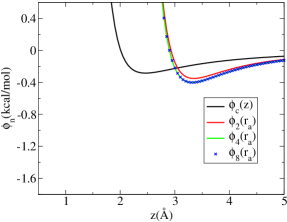
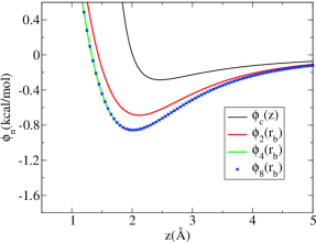
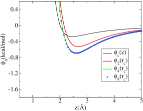
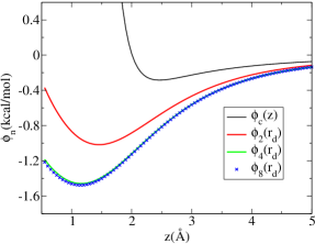
(A) (B) (C) (D)

Figure 1: The potential of a test LJ atom with parameters of the N in the acetonitrile model placed at four different typical sites ($r_{a}$, $r_{b}$, $r_{c}$ and $r_{d}$) on the silica surface. (A) $r_{a}$ is on the top of an oxygen atom. (B) $r_{b}$ is on the top of the middle of two closest oxygen atoms. (C) $r_{c}$ is in the middle of the corresponding $r_{a}$ and $r_{b}$. (D) $r_{d}$ is on the top of the center of an equilateral triangle formed by three closest oxygen atoms. Label for the black line is $\phi_{c}(z)=\phi_{c}(n=1,z)$. See Eq. (2)

The total VdW potential at position ${\mathbf{r}}$ from the whole silica surface including both $n$ layers of explicit atoms and the semi-infinite continuum region is:

$$\phi_{n}({\mathbf{r}})=\sum_{i=1}^{n}\sum_{j=1}^{N_{i}}4\epsilon_{i}\left[\left(\frac{\sigma_{i}}{|{\mathbf{r}}-{\mathbf{r}}_{j}^{i}|}\right)^{12}-\left(\frac{\sigma_{i}}{|{\mathbf{r}}-{\mathbf{r}}_{j}^{i}|}\right)^{6}\right]\\ +\phi_{c}(n+1,z)$$ (2)

where $N_{i}$ is the number of explicit atoms of the $i$-th layer (including periodic images up to a specified cutoff distance) and ${\mathbf{r}}_{j}^{i}$ is the position of the $j$-th atom of the $i$-th layer. A plot of $\phi_{n}({\mathbf{r}})$ with $n$ = 0, 2, 4, and 8 respectively for a test LJ atom with the LJ parameters of N in the acetonitrile model as a function of its distance from the silica surface is shown in Fig. 1.

Figure 1 shows that the potential calculated using four explicit layers overlaps that of eight explicit layers for all positions tested. Clearly, using four explicit layers with a continuum potential is accurate enough to reproduce the VdW potential of the semi-infinite region. Note that noncharged atoms prefer to dock into the position ${\mathbf{r}}_{d}$ rather than the other three because of its lower energy minimum.

The hydrogens in the hydroxylated silica surface used in this work are all attached to the oxygen atoms of the top surface layer (see Fig. 2 (B)). The entire silica surface (all Si atoms and O atoms) is fixed, with the top oxygen layer at the $z=0$ plane, except that hydrogens can freely rotate. The length of O-H bond is constrained to be $1.0{\rm\AA}$ and the Si-O-H harmonic angular bending potential has an equilibrium angle of $109.27$ degrees and a large bending strength of $200.0{\rm kcal/mol}$.

The hydroxylated silica surface has partial charges on the three atoms of the H-O-Si group, which are also taken from the work of Rossky and coworkers Lee_Rossky1994 ; Giovambattista_Rossky2006 . The long-ranged electrostatic interaction has to be treated carefully. We have carried out a test on a pair of ions in a slab-like box with the same length scales used in our simulation of the acetonitrile system (see below) using the exact Ewald2D method Heyes_Clarke1977 , the Ewald3D method, and the corrected Ewald3D method introduced by Yeh and Berkowitz Yeh_Berkowitz1999 . Fig. 3 shows a comparison of these three methods for the test case. Clearly the standard Ewald3D method is very inaccurate but the corrected Ewald3D is in close agreement with the Ewald2D method for separations less than about $100{\rm\AA}$. In what follows we use the corrected Ewald3D method, which is less computationally expensive but quite accurate in the region from $z=0$ to $75{\rm\AA}$.

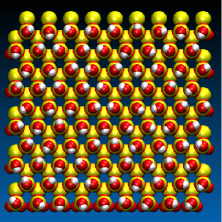
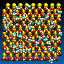
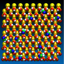
(A) (B) (C) (D)

Figure 2: Side view of the simulation setup (A), with a top view of the hydroxylated silica surface (B). Top views of the CN (C) and CH₃ groups (D) of the first sublayer of acetonitrile molecules docking into the hydroxylated silica surface in a typical configuration as visualized by VMD software vmd1996 are shown.

Figure 3: The electrostatic interaction between two unit point charges computed by three different methods. The simulation setup has a length scale of $l_{z}=150$ Å and $l_{x}=l_{y}=43$ Å.This test case is similar to Figure 4 in reference Yeh_Berkowitz1999 but for the specific length scales used in our simulation.

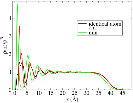
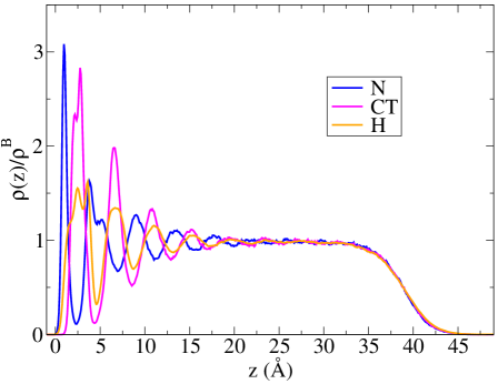
(A)	(B)
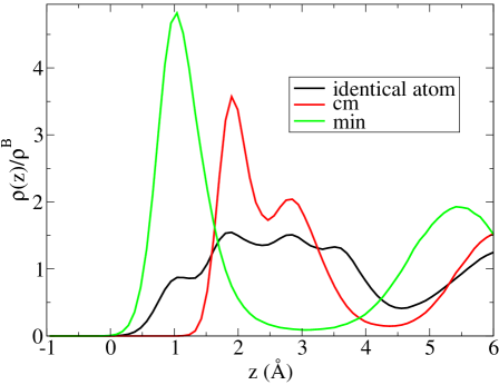
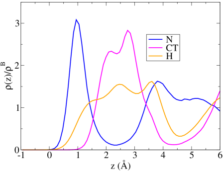
(C)	(D)

Figure 4: Density profiles of the interfacial system defined from positions of all atoms treated as identical, positions of the center of mass, and the minimum position of acetonitrile molecules (A) and positions of the nitrogen atoms, alkyl carbon atoms, and hydrogen atoms of acetonitrile (B). The existence of three qualitatively different regions is evident: a LS region near the silica surface strongly perturbed by the substrate, a bulk liquid-like region from about 22 to 33Å and a LV interface at larger $z$. C and D give an expanded view of A and B respectively from the surface to 6Å . The density is normalized by the bulk value $\rho^{B}$ from a separate bulk simulation. The minimum position of an acetonitrile molecules refers to the minimum z position of all six atoms of the molecule. T=298K and CT stands for the alkyl carbon atom.

II.2 Acetonitrile model and simulation parameters

We performed molecular dynamics simulations of acetonitrile confined in the $z$-direction by two parallel walls using the software DL_POLY version 2.18 dlpoly with modifications to include external potentials and the corrected Ewald3D method to treat the electrostatics. The acetonitrile system studied here consisted of 864 molecules. All acetonitrile molecules were confined by a hydrophobic wall located at $75$Å  and the silica wall with its top oxygen layer located at $0$Å. The potential of the hydrophobic wall had the same form as in Eq. (1) but uses only the repulsive part of the potential Weeks_Chandler_Andersen1971 . Periodic boundary conditions were employed with $L_{x}=45.605$Å, $L_{y}=43.883$Å, and $L_{z}=150$Å. The empty region between $75{\rm\AA}$ and $150{\rm\AA}$ is required for the application of the corrected Ewald3D method (see Fig. 3).

The simulation setup is shown in Fig. 2(B). The acetonitrile potential energy parameters were those previously published by Nikitin and Lyubartsev Nikitin_Lyubartsev2007 . The cutoff distance for the VdW and the short-ranged part of the corrected Ewald simulation was 15Å. The screening parameter for the Ewald summation was 0.26${\rm\AA}^{-1}$. The number of $k$-space vectors for the Ewald summation was 15, 15, and 45 for the $x$, $y$, and $z$ directions respectively. These parameters were optimized choices yielding the best efficiency for our system setup.

A bulk simulation was initially equilibrated at T = 298K and P = 1 atm before putting the acetonitrile on the silica surface. The interfacial system was equilibrated for nearly a nanosecond at constant number of molecules, constant volume and constant temperature T=298K (NVT ensemble) using the Berendsen method Berendsen1984 until no further energy drift was observed. To reduce the computational cost, we first employed a more efficient but less accurate method Wolf1999 ; Chen_Weeks2004 with truncated Coulomb interactions for several hundred picoseconds and then applied the accurate corrected Ewald3D method in the later stage of the equilibration. The latter was also used in all production runs. One NVE production simulation was run for a duration of 300ps using a time step of 1 fs. This was followed by another NVE simulation of 50ps using a time step of 0.5 fs to permit the accurate determination of time correlation functions at very short times. Positions of atoms were recorded at every 5 fs and every 1 fs respectively for further analysis. Total energy is well conserved and no temperature drift was observed in the NVE production simulation.

A separate simulation of the bulk acetonitrile system was carried out for comparison. The production simulation of the bulk system had 864 molecules in a cubic box of size 42.37Å. The number density was $\rho^{B}=0.774{\rm g/cm^{3}}$, which is in good agreement with the experimental value of $\rho=0.777{\rm g/cm^{3}}$ at the temperature T=298K Gallant1969 . A top view of the surface and the first sublayer acetonitrile molecules on the surface is shown in Fig. 2 (B), (C) and (D).

III Results and Discussions

III.1 Singlet densities and orientational profiles

Stable LV and LS interfaces are formed in the simulation of the acetonitrile system and are most simply described by the singlet density profile. However with larger molecules like acetonitrile there are several reasonable choices for which atomic type or molecular position should be used to characterize the location of the molecule in the density profile.

In Fig. 4 we show density profiles defined from positions of the nitrogen (N), methyl carbon (CT), hydrogen (H), center of mass (cm), and minimum $z$ position of any atom in the molecule. We also defined an “identical atom” profile in which all atoms in the molecule are treated as if they were of the same type and we report the spatial distribution of this single atomic species. The average of the number density $\rho(z)$ over the region $25{\rm\AA}<z<30{\rm\AA}$ ($0.98\rho^{B}$) is nearly the same as the bulk density using all definitions and we consider this the bulk region of our interfacial system.

Following previous work Paul_Chandra2005 , the LV interfacial region is defined as the region over which the number density decreases from 90% to 10% of the bulk density. As shown in Fig. 4 (A) and (B), density profiles from all definitions except the minimum position yield almost identical LV interfacial regions ($35.24{\rm\AA}<z<42.08{\rm\AA}$), while the minimum position shifts the LV interfacial region to $34.20{\rm\AA}<z<40.94{\rm\AA}$. The thickness of the LV interface is about $6.7{\rm\AA}$, which is slightly larger than the value $4.7{\rm\AA}$ reported by Paul and Chandra Paul_Chandra2005 using a three-site model of acetonitrile.

As would be expected, the LS density profiles are much more structured than those of the LV interface and have different forms depending on the choice of defining molecular position. Clearly, acetonitrile forms layers on the silica surface from $z=0$ to about $z\simeq 20{\rm\AA}$ and the various profiles provide information about different features of this layering. It is interesting that the indications of the surface-induced layering persist past 20 Å from the substrate. This contrasts with water near silica where perturbations die off by about 10 Å Lee_Rossky1994 , probably indicating the greater orientational flexibility of the tetrahedral hydrogen-bond network.

Most density profiles show shoulder peaks except the density profile based on the minimum position. The first layer of acetonitrile adsorbed on silica is defined as the region from $z=0$ to the first major depletion of density ($z=3{\rm\AA}$ for the minimum position and $z\simeq 4.5{\rm\AA}$ for the identical atom profile and the center of mass profile). The first minimum of the density profile of the nitrogen atom appears at a $z$ distance less than $3{\rm\AA}$ (Fig. 4 (D)), indicating that molecules with the nitrogen atom pointing to the silica surface likely dominate at close distances to the surface.

We further divide the first layer into two sublayers according to the shoulder peak position of the density profile of identical atoms $z=1.2{\rm\AA}$ (Fig. 4 (C)). A top view of the molecules within the sublayer $0<z<1.2{\rm\AA}$ was shown in Fig. 2 (C) and (D). Clearly molecules in the first sublayer prefer to orient with their nitrogen atoms binding to hydrogen atoms (Fig. 2 (C)). About 25% of the sublayer molecules dock into the equilateral triangle formed by three closest oxygen atoms that have their attached hydrogen atoms pointing outside the triangle (Fig. 2 (D)).

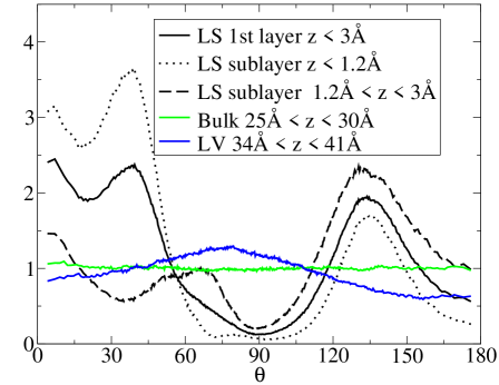
(A)

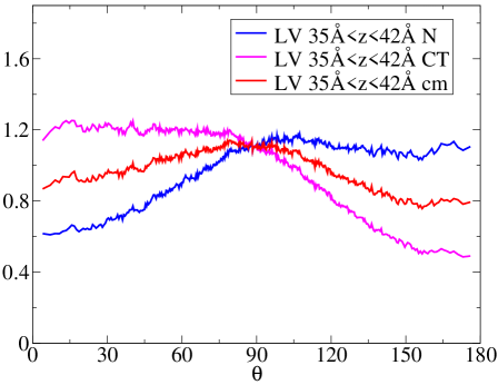
(B)

Figure 5: Orientational profiles of the acetonitrile dipoles relative to the surface normal (positive $z$ direction) when $z$ is the minimum position of the acetonitrile molecules (A) and the orientational profiles of the LV interface when $z$ is the position of nitrogen atom, methyl carbon atom and center of mass (B). The Jacobian factor $\sin\theta$ has been scaled out in all plots of angle distributions, so the bulk system has a uniform distribution. $\theta$ is the angle between the dipole orientation (CT $\leftarrow$ N) and the positive $z$ direction. In our geometry $\theta=0$ implies that the CN group points to the liquid phase at the LV interface and to the silica surface at the LS interface.

Once we have defined the sublayer, the first layer, the bulk region, and the liquid-vapor region according to singlet density profiles, it seems natural to examine the orientational distributions in these regions as shown in Fig. 5 (A). A consistent picture of the LS interface arises from all profiles. The orientation of an acetonitrile molecule in the first layer of the LS region tends to lie in two branches: $\theta<45^{\circ}$ where the nitrogen end points to the surface and around $\theta\simeq 130^{\circ}$ where the nitrogen end points away from the surface. Most molecules within the sublayer $z<1.2$ Å lie in the first branch $\theta<45^{\circ}$ while more molecules in the sublayer $1.2$ Å$<z<3$ Å lie in the second branch so the structure is reminiscent of a lipid bilayer. As the distance between an acetonitrile molecule and the silica surface increases, the orientational distribution gradually approaches unity, where the dipole of a molecule orients randomly as in the bulk.

However, results in the LV interfacial region appear to depend on the choice of singlet density profile. When the location of a molecule is defined by its minimum position as in Fig. 5 (A), the orientational profile has a small maximum at $\theta=90^{\circ}$, parallel to the interface. But Fig. 5 (B) shows that the orientation profile of molecules defined using the positions of N, CT and cm seem to give different interpretations of the preferred molecular orientation at the LV interface. When the position of the center of mass is used, more molecules seem to orient parallel to the interface, consistent with results from the use of the minimum position of molecules in Fig. 5 (A). However, as noted in Cheng_Berne2009 , more CH₃ groups of the acetonitrile molecules appear to point into the liquid (gas) phase if we define the location of an acetonitrile molecule using the position of its nitrogen (carbon) atoms.

We show here that this apparent discrepancy arises from the different contributions of “over-counted” dipoles, arising from the different definitions of molecular position. These considerations become important only when the size of the molecule is a finite fraction of the interface width, and when they are taken into account results from the different definitions can be related to each other.

A molecular $+/-$ dipole is defined as “over-counted” when its positive side (CT atom in the case of acetonitrile) falls into the region of interest ($35$ Å$<z<42$ Å for the LV interface), while its negative side (the N atom in this case) is still located outside of the region, with a similar definition for an over-counted $-/+$ dipole with the negative side inside and positive side outside. The difference shown in Fig. 5 (B) using definitions from the CT atom and N atom can be expressed as $g_{\rm over,+/-}(\theta)-g_{\rm over,-/+}(\theta)$.

The over-counted contribution of $+/-$ dipoles can also be related to the density and angular distribution of the dipoles based on the profile defined using the center of mass position:

$$g_{\rm over,+/-}(\theta)=\left\{\begin{array}[]{c}\frac{\displaystyle\int_{z_{1}-L/2\cos\theta}^{z_{1}+L/2\cos\theta}dz\,\rho_{0}(z)f_{0}(z,\theta)}{\displaystyle\left|\int_{z_{1}}^{z_{2}}dz\,\rho_{+}(z)\right|}\\ \\ \quad\quad\quad\quad{\rm for}\quad 0\leqslant\theta<\pi/2\\ \\ \frac{\displaystyle\int_{z_{2}+L/2\cos\theta}^{z_{2}-L/2\cos\theta}dz\,\rho_{0}(z)f_{0}(z,\theta)}{\displaystyle\left|\int_{z_{1}}^{z_{2}}dz\,\rho_{+}(z)\right|}\\ \\ \quad\quad\quad\quad{\rm for}\quad\pi/2\leqslant\theta\leqslant\pi\end{array}\right.$$ (10)

where $L$ is the length of the dipole (distance between CT and N). Here $\rho_{0}(z)$ is the density profile defined using the center of mass position and $\rho_{+}(z)$ is the profile when the location of the molecule is defined according to its atom with positive charge (these functions closely resemble each other and either can be used in the calculation). $f_{0}(z,\theta)d\theta$ is the probability for a given dipole with its center located at position $z$ having orientational angle in $[\theta,\theta+d\theta]$. When $+/-$ and $z_{1}/z_{2}$ are exchanged simultaneously, Eq. (10) then gives the contribution of over-counted $-/+$ dipoles.

In order to check the validity of Eq. (10), we first calculate the average orientational distribution around $z=z_{1}$ and $z=z_{2}$ as shown in Fig. 6 (A). Figure 6(B) shows the comparison between the calculation from Eq. (10) (red dashed line) when the average orientational distribution is used as the input and when the explicit histogram distribution of the overcounted molecules is used (solid black line). The overlap between the two lines confirms the validity of Eq. (10). In fact, Eq. (10) can be accurately approximated in this case by simply taking $f_{0}(z,\theta)=1$. The computed over-counted contributions are barely changed. As shown in Fig. 6(B), Eq. (10) gives an excellent description of the simulation results.

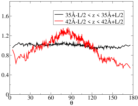
(A)

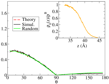
(B)

Figure 6: Orientational profile of molecules at the boundaries around $z_{1}=35{\rm\AA}$ and $z_{2}=42{\rm\AA}$ (A) and contribution from the over-counted $+/-$ molecules to the orientational distribution (B). The black solid line (Simul.) in (B) is computed from the histogram of the over-counted molecules. The red dashed line (Theory) in (B) is computed through Eq. (10) using $\rho_{+}(z)\simeq\rho_{0}(z)$, shown in the inset of (B) (see also Fig. 4), and $f_{0}(z,\theta)$ shown in (B) with $z_{1}=35{\rm\AA}$, $z_{2}=42{\rm\AA}$ and $L=2.6{\rm\AA}$. The green solid line (Random) in (B) is computed in the same way as the red dashed line except that $f_{0}(z,\theta)=1$.

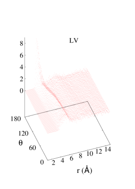
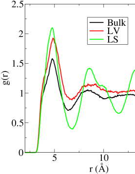
(A) (B) (C) (D)

Figure 7: Radial angular distribution $g_{cm}(r,\theta)$ at T = 298K for the first layer LS region (A), the bulk liquid region (B), the interfacial LV region (C), and the results after angular integration over $\theta$ (D). The center of mass position is used for the definition of three different regions. $\theta$ is the angle between the dipole axis of two molecules and $r$ is the distance between the center of mass positions of the two molecules.

Clearly, because the number of over-counted molecules at the high density side $z=z_{1}$ of the LV interface cannot be compensated by those at the low density side $z=z_{2}$ and the magnitude of $g_{\rm over,+/-}(\theta)$ is non-negligible, the orientational profiles computed from different definitions of the position of a molecule in the interface give apparently contradictory predictions for the prefered orientation of the molecules.

In the case of a bulk system, the over-counting from the two boundaries exactly cancels each other and $g_{\rm over,+/-}(\theta)=g_{\rm over,-/+}(\theta)$. In the case of the LS interface, because values of $\rho_{0}(z)$ in the numerator of Eq. (10) is much smaller than the average density of the interfacial region (e.g. $\rho_{0}(z=4.5{\rm\AA})\simeq 0)$, the magnitude of $g_{\rm over,+/-}$ is very small and makes almost no contribution to the overall orientational profile in the interfacial region (e.g. the first layer orientational profile). Therefore, there is little discrepancy for cases of bulk and solid-liquid interfacial systems.

In case of the LV interface, when the length of the dipole (e.g. $L=2.6{\rm\AA}$ for an acetonitrile molecule) is comparable to the interfacial width (e.g. $z_{2}-z_{1}\simeq 7{\rm\AA})$, $g_{\rm over,-/+}$ is asymmetric and the over-counted molecules from the dense boundaries can make a significant contributions to the overall distribution and thus generate an apparent discrepancy. These considerations should be taken into account in interpretations of simulation or experimental data.

III.2 Correlated structural properties

Although singlet density and orientational profile have been studied in previous work Morales_Thompson2009 ; Paul_Chandra2005 , correlated structures are seldom investigated. In order to shed light on how the antiparallel correlation Nikitin_Lyubartsev2007 between two acetonitrile molecule changes due to the effect of inhomogeneity, we define a quantity called the radial angular distribution function:

$$g_{cm}(r,\theta)=\frac{1}{N_{c}}\sum_{i=1}^{N_{c}}\sideset{}{{}^{\prime}}{\sum}_{j=1}^{N_{c}}\left<\delta(r-r_{ij})\delta(\theta-\theta_{ij})\right>,$$ (11)

where $N_{c}$ is the number of particles contained in the three different regions defined above: the bulk region, LV region, and the first layer of the LS region. The $g_{cm}(r,\theta)$ is essentially the normalized histogram over independent pairs of molecular dipoles in the three regions of interest; the prime on the sum indicates that terms with $i=j$ are excluded. Here $r_{ij}$ is the distance between the center of mass of the $i$-th and $j$-th molecule and $\theta_{ij}$ is the angle between the dipole orientations of the two molecules. The radial angular correlation function is normalized to $1$ at large distance $r$ and the integral over $\theta$ gives the usual center of mass radial distribution function.

Fig. 7 shows that acetonitrile at the LV interface has an even stronger antiparallel correlation than in the bulk. In contrast, molecules in the first layer of the LS interfacial region completely lose the preferred correlation at $\theta=180^{\circ}$. The silica surface not only aligns the singlet molecular orientation such that it prefers to point toward the normal of the surface (Fig. 5(A)), but it also significantly destroys the strong anti-parallel pair correlations seen for bulk liquid acetonitrile. At the free liquid-vapor interface, the singlet orientation differs only slightly from that of the random distribution in the bulk. The dominant intermolecular interactions cause LV interfacial molecules to preferentially orient in an antiparallel manner. But local interactions from the silica surface are strong enough to significantly modify the pair structure of molecules in the first layer. Since solid acetonitrile has even stronger anti-parallel correlations that would be similarly disrupted at the silica surface this, along with the general modification of bulk structure at a surface, could provide a possible explanation for the decrease of the melting point when acetonitrile is confined in silica pores.

III.3 Singlet and collective rotational dynamics

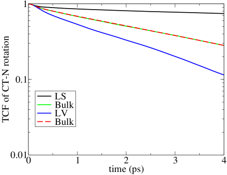
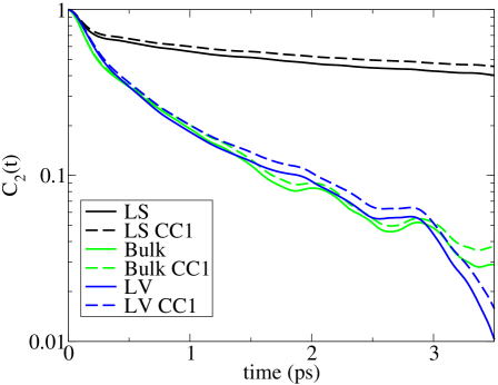
(A) (B)

Figure 8: Singlet (A) and collective (B) reorientational correlations for acetonitrile in different regions. See Eqs. (12) and  (16). The red dashed line in (A) is computed from a separate simulation of the bulk system. Dashed lines in (B) are the corresponding CC1 model calculations. Rotational time scales obtained by linear fit of the logarithm plot after $t>2{\rm ps}$ are shown in Table 1. The definition of different regions is the same as in Fig. 5.

Both singlet and collective rotational dynamics are of interest as they can be measured from spectroscopic experiments Loughnane_Fourkas1999 ; Kittaka2007 . The time correlation function (TCF) of the rotation of the symmetrical axis (CT-N) is defined as

$$C(t)=\frac{1}{N_{c}}\sum_{i=1}^{N_{c}}\left<{\mathbf{v}}_{i}(0)\cdot{\mathbf{v}}_{i}(t)\right>,$$ (12)

where ${\mathbf{v}}_{i}$ is the rotational axis of the $i$-th molecule and $N_{c}$ is the total number of molecules counted in particular region of interest. The collective reorientational behavior of the bulk acetonitrile system has been studied by Ladanyi and coworkers Elola_Ladanyi2005 but few workers have addressed the collective dynamics of interfacial or confined systems.

The collective polarizability $\overline{\Pi}$ of a group of molecules is the sum of polarizabilities of each molecule. The standard point dipole/induced point dipole (DID) model expresses the individual polarizability $\overline{\pi}(j)$ for molecule $j$ as a sum of a molecular component (gas-phase polarizability $\overline{\alpha}(j)$) and an interaction-induced component

$$\overline{\pi}(j)=\overline{\alpha}(j)+\overline{\alpha}(j)\cdot\sum_{k\not=j}^{N}\overline{T}_{jk}\cdot\overline{\pi}(k),$$ (13)

where the dipole-dipole tensor $\overline{T}_{jk}$ between molecule $j$ and $k$ can be written as

$$\overline{T}_{jk}=\frac{1}{r^{3}}\left.(3\hat{r}\hat{r}-\overline{\rm I})\right|_{{\mathbf{r}}={\mathbf{r}}_{jk}}$$ (14)

and $\hat{r}={\mathbf{r}}/r$ is the unit vector along the direction ${\mathbf{r}}$. Eq. (13) can be solved self-consistently or by matrix inversion Applequist1972 . An efficient first-order approach (CC1) corresponds to replacing $\overline{\pi}(k)$ on the right hand side of Eq, (13) by the gas-phase polarizability $\overline{\alpha}(k)$ Elola_Ladanyi2005 .

The total collective polarizability $\overline{\Pi}$ for a region of $N_{c}$ molecules is

$$\overline{\Pi}=\sum_{j}^{N_{c}}\overline{\pi}(j)=\overline{\Pi}_{0}\overline{\rm I}+\overline{\Pi}_{2},$$ (15)

where $\overline{\Pi}_{0}$ and $\overline{\Pi}_{2}$ are the isotropic and anisotropic polarizability of the region of $N_{c}$ molecules respectively. Different from the bulk system, the average of the $xz$ or $yz$ component of the anisotropic polarizability in the nonuniform system we study here is not zero. In order to focus on just the relaxation part of the anisotropic collective polarizability, we define the TCF $C_{2}(t)$ as

$$C_{2}(t)=\left<{\rm Tr}[(\overline{\Pi}_{2}(0)-\left<\overline{\Pi}_{2}\right>)\cdot(\overline{\Pi}_{2}(t)-\left<\overline{\Pi}_{2}\right>)]\right>$$ (16)

Analysis of $C_{2}(t)$ is crucial because it is directly relevant to the OKE signal McMorrow_Kenney-Wallace1988 ; Geiger_Ladanyi1989 ; Hu_Margulis2008 . The notation used in this subsection is the same as the work by Hu et. al. Hu_Margulis2008 . The TCFs of anisotropic collective polarizability for different regions of our system are primarily studied here using both the all-order and first order DID model. The gas phase polarizabilities of acetonitrile used here are $\alpha_{\parallel}=5.80$ ų and $\alpha_{\perp}=3.65$ ų Geiger_Ladanyi1989 . The polarization effect from the atoms of the silica surface is not considered here.

Table 1: Estimate of singlet and collective rotational time scales for acetonitrile in different regions.

axis/model	LS 1st layer	Bulk region	LV region
CT-N	24(4) ps	3.4(2) ps	1.9(1) ps
Collective	8.1(2) ps	1.4(1) ps	1.1(1) ps
CC1	9.6(2) ps	1.5(1) ps	1.2(1) ps

Fig. 8 shows the singlet and collective reorientation correlations in a logarithmic plot. A separate calcuation of $C(t)$ from the simulation of bulk acetonitrile (red dashed line in Fig. 8(A)) overlaps the corresponding $C(t)$ for the bulk region in the inhomogeneous system. The rotational time scale in the region with a distance of larger than $25$Å from the surface is almost the same as in the bulk. This finding is consistent with the experiment work of Kittaka and coworkers Kittaka2005 . Comparison between the all-order calculations and the first order approximation in Fig. 8 (B) shows that the effect of the higher orders is almost negligible in the bulk and in the LV region, consistent with the work of Elola and Ladanyi Elola_Ladanyi2005 .

Higher order effects are a little more important for the collective reorientation of molecules in the first layer close to the silica surface. The values of the rotational time scales determined by fitting the long time behavior (2-4 ps for singlet rotations and 2-3.5 ps for collective rotations) to an exponential form are shown in Table 1. The value of the time scale for the self-rotational correlation in the bulk and LV region are $\tau_{\rm B}=$ 3.4ps and $\tau_{\rm LV}=$ 1.9ps respectively. These values are different from those reported by Paul and Chandra Paul_Chandra2005 , 10.75ps and 5.75ps respectively, because they determined the orientational relaxation time scale from the time integral of the correlation function, and finite size and equilibration effects would be expected to affect both these estimates in different ways. Both work agrees however that the reorientational motion has been significantly enhanced at the LV interface relative to the bulk phase.

Both singlet and collective reorientation of the first layer of acetonitrile close to the silica surface are highly hindered. However, the collective reorientation in the first layer is much faster than the self-rotation of a molecule in the same region. Fourkas and coworkers measured the collective reorientation time scales in the bulk and in the pores as 1.66ps and 26ps respectively at T=290K and 1.42ps and 19ps respectively at T=309K Loughnane_Fourkas1999a . We estimated the experimental values for T=298K, 1.54ps and 22 ps by simply taking the average of the values at the higher and lower temperatures.

Thus, our calculated bulk value 1.39ps is about 10% smaller than the experimental value 1.54ps. Because experiments on acetonitrile in pores measure components arising from both bulk-like and surface molecules, and can be affected by other aspects of the confinement, our computed time scale for the collective reorientation of the first layer LS acetonitrile, 8.1ps seems in reasonable qualitative agreement with the reported experimental value of about 22ps. However, a quantitative understanding of the different time scales in the OKE experiment and test of the triexponential model used Loughnane_Fourkas1999a would require a similar theoretical investigation of the OKE signals in silica pores, which is beyond the scope of this paper.

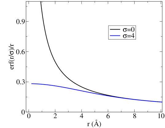
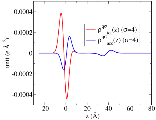
(A) (B) (C) (D)

Figure 9: Separation of the electrostatic interactions. (A) The potential from a point charge ($\sigma=0$) and from a Gaussian charge distribution with width $\sigma=4$. (B) The bare charge density of the mobile acetonitrile molecules and the corresponding smooth charge density. (C) The comparison between the smooth charge densities of the total system and the mobile acetonitrile molecules. (D) The total force in $z$ direction and its long-ranged part. The insets show the acetonitrile charge densities (B) and the total force (D) in the region of the LV interface. Smoothing eliminates the simulation noise still visible in the bare results. The blue lines in (B) and (C) are the same but on different scales. See Eqs. (22),  (23) and  (26).

III.4 Electrostatic potential and the long range contribution

In order to shed light on the importance of the correct treatment of the long-ranged electrostatics in this interfacial system, we analyze the total equilibrium charge density $\rho^{q}_{\rm tot}({\mathbf{r}})$, comprised of the fixed charges in the silica substrate and the induced equilibrium mobile charge density $\rho^{q}_{\rm ace}(\mathbf{r})$ in the acetonitrile fluid. The associated electrostatic potentials are given by Poisson’s equation (in Gaussian units) as

$$\mathcal{V}^{\rm tot}(\mathbf{r})=\int d\mathbf{r}^{\prime}\,\rho^{q}_{\rm tot}(\mathbf{r}^{\prime})\cdot\frac{1}{\left|\mathbf{r}-\mathbf{r^{\prime}}\right|}.$$ (17)

and

$$\mathcal{V}^{\rm ace}(\mathbf{r})=\int d\mathbf{r}^{\prime}\,\rho^{q}_{\rm ace}(\mathbf{r}^{\prime})\cdot\frac{1}{\left|\mathbf{r}-\mathbf{r^{\prime}}\right|}.$$ (18)

In other work Chen_Weeks2004 ; Rodgers_Weeks2008 , we have argued for the utility of splitting the basic Coulomb $1/r$ interaction appearing in Eqs. (17) and (18) into short- and long-ranged parts based on a “smoothing length” $\sigma$ of order a characteristic nearest neighbor spacing:

$$\frac{1}{r}=v_{0}(r)+v_{1}(r)=\frac{{\rm erfc}(r/\sigma)}{r}\ +\frac{{\rm erf}(r/\sigma)}{r}.$$ (19)

Here $v_{1}(r)$ is the functional form associated with the electrostatic potential due to a unit Gaussian charge distribution of width $\sigma$, defined as

$$\rho_{G}(\mathbf{r})=\frac{1}{\pi^{3/2}\sigma^{3}}\exp\left(-\frac{r^{2}}{\sigma^{2}}\right),$$ (20)

implying a $v_{1}(r)$ given by the convolution

$$v_{1}(r)\equiv\int d\mathbf{r}^{\prime}\rho_{G}(\mathbf{r^{\prime}})\cdot\frac{1}{\left|\mathbf{r}-\mathbf{r^{\prime}}\right|}=\frac{\mathop{\rm erf}(r/\sigma)}{r}~{}.$$ (21)

As shown in Fig. 9(A), $v_{1}(r)$ is slowly-varying in $r$-space over the length scale $\sigma$.

We showed in Ref. Hu_Weeks2009 that for bulk acetonitrile the forces from the long-ranged parts of the Coulomb interactions essentially cancel when $\sigma$  is properly chosen to be $4$Å, and a very accurate description of local pair correlations arises from considering the simpler “strong-coupling” system with only truncated Coulomb interactions $v_{0}(r)$. Moreover, as argued in Ref. Rodgers_Weeks2008 ; Rodgers_Weeks2008a , in nonuniform systems, where this force cancellation does not occur, the charge densities that best reflect the long-ranged electrostatics are not the bare densities $\rho^{q}_{\rm tot}(\mathbf{r})$ and $\rho^{q}_{\rm ace}(\mathbf{r})$ appearing in Eqs. (17) and (18) but rather the Gaussian-smoothed charge densities

$$\rho^{q\sigma}_{\rm tot}(\mathbf{r})\equiv\int d\mathbf{r}^{\prime}\,\rho^{q}_{\rm tot}(\mathbf{r}^{\prime})\rho_{G}(\left|\mathbf{r}-\mathbf{r^{\prime}}\right|),$$ (22)

and

$$\rho^{q\sigma}_{\rm ace}(\mathbf{r})\equiv\int d\mathbf{r}^{\prime}\,\rho^{q}_{\rm ace}(\mathbf{r}^{\prime})\rho_{G}(\left|\mathbf{r}-\mathbf{r^{\prime}}\right|),$$ (23)

generated from Eqs. (17), (18) and (21) when only the long-ranged Coulomb component $v_{1}(\left|\mathbf{r}-\mathbf{r^{\prime}}\right|)$ is used:

$$\mathcal{V}_{1}^{\rm tot}(\mathbf{r},\sigma) \equiv \int d\mathbf{r}^{\prime}\,\rho^{q}_{\rm tot}(\mathbf{r}^{\prime})\cdot v_{1}(\left|\mathbf{r}-\mathbf{r^{\prime}}\right|)$$ (24)

$$= \int d\mathbf{r}^{\prime}\,\rho^{q\sigma}_{\rm tot}(\mathbf{r}^{\prime})\cdot\frac{1}{\left|\mathbf{r}-\mathbf{r^{\prime}}\right|}.$$

and

$$\mathcal{V}_{1}^{\rm ace}(\mathbf{r},\sigma) \equiv \int d\mathbf{r}^{\prime}\,\rho^{q}_{\rm ace}(\mathbf{r}^{\prime})\cdot v_{1}(\left|\mathbf{r}-\mathbf{r^{\prime}}\right|)$$ (25)

$$= \int d\mathbf{r}^{\prime}\,\rho^{q\sigma}_{\rm ace}(\mathbf{r}^{\prime})\cdot\frac{1}{\left|\mathbf{r}-\mathbf{r^{\prime}}\right|}.$$

for the total system and the mobile acetonitrile molecules respectively.

Thus we are able to rationalize the contribution of the long-ranged part of the electrostatics through analysis of the smooth charge density $\rho^{q\sigma}_{\rm tot}(\mathbf{r})$ and the corresponding electrostatic potential $\mathcal{V}_{1}^{\rm tot}(\mathbf{r},\sigma)$. One virtue of this perspective is that because of the integration over the smoothing length $\sigma$, $\rho^{q\sigma}_{\rm tot}(\mathbf{r})$ is very slowly varying along the interface in the $x$ and $y$ directions, unlike the bare charge density. As a result, $\mathcal{V}_{1}^{\rm tot}(\mathbf{r},\sigma)=\mathcal{V}_{1}^{\rm tot}(z,\sigma)$ to a very good approximation Rodgers_Weeks2008 ; Rodgers_Weeks2008a and we can focus only on forces in the $z$-direction given by:

$$F_{z}(z,\sigma)=-\frac{\partial\mathcal{V}_{1}^{\rm tot}(z,\sigma)}{\partial z}.$$ (26)

A plot of $\rho^{q\sigma}_{\rm tot}(z)$, $\rho^{q\sigma}_{\rm ace}(z)$ and $F_{z}(z,\sigma)$ is shown in Fig. 9. The magnitude of the acetonitrile charge density close to silica surface ($0<z<10$ Å) is on the order of $0.01$ e Å^-3 and it dramatically reduces to the order of $0.0001$ e Å^-3 at the LV interface. The smoothed charge density in the LS region for the relevant $\sigma=4.0$ Å is much smaller, with a magnitude of order of only $0.0002$ e Å^-3.

This implies that the long-ranged ($\sigma=4$ Å) part of the charge density only contributes 4% to the total charge density in the region of LS interface. Nevertheless, the long-ranged forces play an important role in properly describing the surface-induced dipole, as discussed in detail in Ref.  Rodgers_Weeks2008, and illustrated below. However, in the LV interfacial region, the bare charge density is much smaller, and the long-ranged ($\sigma=4$ Å) charge density can contribute as much as 50% (see the inset of Fig. 9 (B)). Analysis of the force in the $z$ direction (Fig. 9 (D)) supports this same conclusion. Therefore, the long-ranged part of the electrostatics plays a relatively more important role in determining the structure and dynamics of acetonitrile in the LV interface than near the LS interface, where most aspects of the local structure is dominated by short-ranged forces.

Fig. 9 (C) shows a comparison of the total smooth charge density (red) and the smooth charge density of the mobile acetonitrile molecule only (blue). The overlap of the two densities at distances larger than $10$ Å indicates complete screening of the induced surface dipole beyond about $10$ Å, consistent with our finding in previous subsections that the dynamics and structure of acetonitrile in the region between $25$ Å and $30$ Å have reached the bulk limit.

IV Conclusion

We have investigated the structure and dynamics of the acetonitrile system on silica surface and at its LV interface. The change of melting point, the slowing down of dynamics for molecules close to silica surface and the tilting angle of the molecule at the LV interface were all explained in detail through our studies of structure and dynamics. The antiparallel correlations in the LS (LV) region was weaker (stronger) than in the bulk. Both singlet and collective reorientational time scales in the first layer close to the silica surface are approximately $6-7$ times slower than the corresponding time scales in the bulk. The collective reorientational time scale is about 3 times faster than that of the singlet reorientation. Moreover, we provide a general explanation of the ambiguity that arises in determining the orientational profile using interfaces defined with different choices of the atoms in a molecular system. Our current study of the acetonitrile system provides a general framework for future MD simulations of LS and LV interfacial systems. We plan to investigate other typical systems such as quadrupolar (carbon dioxide), dipolar (propionitrile) and associating fluids (hydrogen fluoride and water) on the silica surface and at their liquid-vapor interfaces.

References

- (1) Nikiel, L.; Hopkins, B.; Zerda, T. W. J. Phys. Chem. 1990, 94, 7458–7464.
- (2) Zhang, D.; Gutow, J. H.; Eisenthal, K. B.; Heinz, T. F. J. Chem. Phys. 1993, 98, 5099–5101.
- (3) Zhang, J.; Jonas, J. J. Phys. Chem. 1993, 97, 8812–8815.
- (4) Tanaka, H.; Iiyama, T.; Uekawa, N.; Suzuki, T.; Matsumoto, A.; Gr n, M.; Unger, K. K.; Kaneko, K. Chem. Phys. Lett. 1998, 293, 541 – 546.
- (5) Loughnane, B. J.; Farrer, R. A.; Fourkas, J. T. J. Phys. Chem. B 1998, 102, 5409–5412.
- (6) Loughnane, B. J.; Scodinu, A.; Farrer, R. A.; Fourkas, J. T.; Mohanty, U. J. Chem. Phys. 1999, 111, 2686–2694.
- (7) Loughnane, B. J.; Farrer, R. A.; Scodinu, A.; Fourkas, J. T. J. Chem. Phys. 1999, 111, 5116–5123.
- (8) Kim, J.; Chou, K.; Somorjai, G. J. Phys. Chem. B 2003, 107, 1592–1596.
- (9) Kittaka, S.; Iwashita, T.; Serizawa, A.; Kranishi, M.; Takahara, S.; Kuroda, Y.; Mori, T.; Yamaguchi, T. J. Phys. Chem. B 2005, 109, 23162–23169.
- (10) Kittaka, S.; Kuranishi, M.; Ishimaru, S.; Umahara, O. J. Chem. Phys. 2007, 126, 091103.
- (11) Morales, C. M.; Thompson, W. H. J. Phys. Chem. A 2009, 113, 1922–1933.
- (12) Mountain, R. D. J. Phys. Chem. B 2001, 105, 6556–6561.
- (13) Paul, S.; Chandra, A. J. Phys. Chem. B 2005, 109, 20558–20564.
- (14) Gulmen, T. S.; Thompson, W. H. Langmuir 2009, 25, 1103–1111.
- (15) Cheng, L.; Paramore, S.; Berne, B. J. private communication.
- (16) Lee, S. H.; Rossky, P. J. J. Chem. Phys. 1994, 100, 3334–3345.
- (17) Giovambattista, N.; Rossky, P. J.; Debenedetti, P. G. Phys. Rev. E 2006, 73, 041604.
- (18) Giovambattista, N.; Debenedetti, P.; Rossky, P. J. Phys. Chem. C 2007, 111, 1323–1332.
- (19) Giovambattista, N.; Debenedetti, P.; Rossky, P. J. Phys. Chem. B 2007, 111, 9581–9587.
- (20) Giovambattista, N.; Rossky, P. J.; Debenedetti, P. G. Phys. Rev. Lett. 2009, 102, 050603.
- (21) Ding, F.; Hu, Z.; Zhong, Q.; Manfred, M.; Gattass, R. R.; Brindza, M. R.; Fourkas, J. T.; Walker, R. W.; Weeks, J. D. to be published.
- (22) Yeh, I.-C.; Berkowitz, M. L. J. Chem. Phys. 1999, 111, 3155–3162.
- (23) Heyes, D.M.; Barber, M.; M. B.; Clarke, J. H. R. J. Chem. Soc., Faraday Trans. 2 1977, 73, 1485–1496.
- (24) http://cst-www.nrl.navy.mil/lattice/struk/c9.html.
- (25) Nikitin, A. M.; Lyubartsev, A. P. J. Comp. Chem. 2007, 28, 2020–2026.
- (26) Humphrey, W.; Dalke, A.; Schulten, K. J. Mol. Graphics 1996, 14, 33–38.
- (27) Smith W.; Yong C.; Rodger P. Molec. Sim. 1996 28, 385 471.
- (28) Weeks, J. D.; Chandler, D.; Andersen, H. C. J. Chem. Phys. 1971, 54, 5237–5247.
- (29) Berendsen, H. J. C.; Postma, J. P. M.; van Gunsteren, W. F.; DiNola, A.; Haak, J. R. J. Chem. Phys. 1984, 81, 3684–3690.
- (30) Wolf, D.; Keblinski, P.; Phillpot, S. R.; Eggebrecht, J. J. Chem. Phys. 1999, 110, 8254–8282.
- (31) Chen, Y.-G.; Kaur, C.; Weeks, J. J. Phys. Chem. B 2004, 108, 19874–19884.
- (32) Gallant, R. W. Hydrocarb Proc. 1969, 48, 135.
- (33) Elola, M. D.; Ladanyi, B. M. J. Chem. Phys. 2005, 122, 224506.
- (34) Applequist, J.; Carl, J. R.; Fung, K. J. Am. Chem. Soc. 1972, 94, 2952–2960.
- (35) McMorrow, D.; Lotshaw, W. T.; Kenney-Wallace, G. A. IEEE J. Quantum Electron. 1989, 24, 443–454.
- (36) Geiger, L. C.; Ladanyi, B. M. Chem. Phys. Lett. 1989, 159, 413–420.
- (37) Hu, Z.; Huang, X.; Annapureddy, H. V. R.; Margulis, C. J. J. Phys. Chem. B 2008, 112, 7833-7849.
- (38) Rodgers, J. M.; Weeks, J. D. Proc. Nat. Acad. Sci. (USA) 2008, 105, 19136–19141.
- (39) Hu, Z.; Rodgers, J.; Weeks, J. to be published.
- (40) Rodgers, J. M.; Weeks, J. D. J. Phys.: Cond. Matt. 2008, 20, 494206.