Open-Loop Spatial Multiplexing and Diversity Communications in Ad Hoc Networks

Abstract

This paper investigates the performance of open-loop multi-antenna point-to-point links in ad hoc networks with slotted ALOHA medium access control (MAC). We consider spatial multiplexing transmission with linear maximum ratio combining and zero forcing receivers, as well as orthogonal space time block coded transmission. New closed-form expressions are derived for the outage probability, throughput and transmission capacity. Our results demonstrate that both the best performing scheme and the optimum number of transmit antennas depend on different network parameters, such as the node intensity and the signal-to-interference-and-noise ratio operating value. We then compare the performance to a network consisting of single-antenna devices and an idealized fully centrally coordinated MAC. These results show that multi-antenna schemes with a simple decentralized slotted ALOHA MAC can outperform even idealized single-antenna networks in various practical scenarios.

The work of M. R. McKay was supported by the Hong Kong Research Grants Council (RGC) General Research Fund under grant no. 617809.

The material in this paper was presented in part at the IEEE International Conference on Communications, Beijing, China, May 2008, and the IEEE International Conference on Communications, Dresden, Germany, July 2009.

I Introduction

Multiple antennas offer the potential for significant performance improvements in wireless communication systems by providing higher data rates and more reliable links. A practical method which can achieve high data rates is to employ spatial multiplexing transmission in conjunction with low complexity linear receivers, such as maximum ratio combining (MRC) or zero forcing (ZF) receivers. In the context of point-to-point systems operating in the absence of interference, the performance of such techniques has now been well studied (see e.g., [1, 2]). Multiple antennas can also be used to provide more reliable links through spatial diversity techniques. Of the various spatial diversity techniques which have been proposed, orthogonal space time block codes (OSTBC) have emerged as one of the most important practical approaches, since they offer high diversity gains, whilst requiring only very low computational complexity. The performance of OSTBC techniques have also been well studied in the context of point-to-point systems, operating in the absence of interference (see e.g., [3, 4], and references therein).

In this paper, we investigate spatial multiplexing techniques and OSTBC in the context of wireless ad hoc networks using a slotted ALOHA medium access control (MAC) protocol. The interference model we use includes the spatial distribution of nodes, with the nodes distributed as a homogeneous Poisson point process (PPP) on the plane. Besides approximating realistic network scenarios, modeling the nodes according to a PPP has the benefit of allowing network performance measures to be obtained. This model has been used previously in [5] which considered code division multiple access (CDMA) systems, and in [6] which considered single-antenna systems with threshold scheduling and power control. It was also used in [7], where network performance measures for a single antenna coordinated MAC protocol were derived.

The PPP model has also been extended to ad hoc networks employing multiple antennas at each transmitting and receiving node. In particular, the schemes in [8, 9, 10, 11] considered the use of the receive antennas to cancel interference from the $L$ closest nodes to the receiver. However, a key requirement of these schemes is that each receiver must measure the channels of the $L$ closest interfering nodes, or at least the corresponding short-term covariance information, the practical feasibility of which is still not clear. In contrast, the schemes in [12, 13, 14, 15] considered the use of the receive antennas for either canceling self-interference or increasing the signal power from the corresponding transmitter only, and as such, require the receiver to estimate only the transmitter-receiver channel (something which can be done with standard channel estimation techniques). For this scenario, [12] considered various spatial diversity techniques, and derived transmission capacity and outage probability expressions. In [13, 14], the multiple antennas were used for spatial multiplexing, assuming a “closed-loop” scenario where channel knowledge is available at the transmitter. In particular, [13] considered multiple-input multiple-output (MIMO) singular value decomposition systems, whereas [14] considered MIMO broadcast transmission, for which each transmitting node communicated independently with multiple receiver nodes. Note that all of these papers, with the exception of [12, 15], assumed that either the receiver can acquire knowledge about the network interference, or that there is sufficient capabilities for each receiver to feedback channel information back to their corresponding transmitter. In practice, it seems reasonable to investigate simpler techniques which do not require the receiver to constantly measure the network interference, nor require the transmitter to have channel information. We refer to such schemes as point-to-point “open-loop” schemes.

One previous contribution which focuses on such schemes is provided in [15], where OSTBC and spatial multiplexing with ZF receivers were considered, and approximations were derived for the frame-error probability. In general, however, the fundamental question as to whether to use open-loop spatial multiplexing or diversity-based transmission in ad hoc networks, particularly from a capacity-based network performance point of view, is not well understood.

In this paper, we derive new network performance measures for point-to-point open-loop spatial multiplexing with MRC and ZF receivers, and OSTBC, using a slotted ALOHA MAC, and the same PPP ad hoc network model as in [5, 12]. In all cases, we do not require the receiver to know the network interference, and the transmitter does not have any channel state information. (Note that for the ZF case, each receiver cancels interference from its corresponding transmitter only.) We derive new closed-form expressions for the outage probability, network throughput, and transmission capacity. For spatial multiplexing, these results are exact; whereas, for OSTBC, they are accurate approximations, which we show to be significantly more accurate than previous corresponding approximations.

Our analytical results reveal key insights into the relative throughput performance of spatial multiplexing with MRC and ZF receivers, as well as OSTBC, demonstrating that each scheme may outperform the other, depending on different network parameters such as the node intensity and the chosen signal-to-interference noise ratio (SINR) operating value $\beta$. We also gain insights into the optimal number of transmit antennas to employ for each scheme. For certain scenarios, e.g., sufficiently dense networks or networks with high operating SINR values, these insights are obtained analytically. For example, we show that single-stream transmission is throughput-optimal in dense networks and for networks operating with high $\beta$ requirements, and that transmitting the maximum number of data streams is throughput-optimal for systems operating with low $\beta$ requirements.

We then analyze the transmission capacity of the spatial multiplexing and OSTBC systems. Among other things, we prove that for spatial multiplexing, the transmission capacity can scale linearly with the number of antennas, and we derive precise conditions which must be met to achieve this scaling, using tools from large-dimensional random matrix theory. We also provide concrete design guidelines for selecting the number of transmit streams for achieving (and maximizing) this scaling, and contrast our results with those in [10], which derived a similar scaling result with receivers employing (network) interference cancelation. In addition, we prove that the transmission capacity of OSTBC scales only sub-linearly with the number of antennas, regardless of the particular code employed.

Finally, we turn from the analysis and comparison of different MIMO schemes to look closer at the benefits of multiple antennas with a decentralized MAC, compared with the benefits of a tightly coordinated MAC. In particular, we compare the performance of a multi-antenna system employing a simple slotted ALOHA MAC protocol with a baseline scheme involving single-antenna devices and a fully coordinated access (CA) MAC which enforces guard zones around each receiver. This scheme is similar to that proposed in [7], however we also consider a time division multiple access (TDMA) scheme where only one transmitting node around each receiver within the guard zone is scheduled to transmit. It is worth noting that this is an idealized protocol, since the overhead involved in achieving full coordination is prohibitive in practice for ad hoc networks. To compare with this baseline scheme, we first derive new throughput expressions for the CA MAC protocol. These expressions allow us to show the important result that the slotted ALOHA approach with multiple antennas can actually perform better than the idealized CA MAC, for a wide range of system parameters. This shows that not only does the use of multiple antennas compensate for the inherent performance loss caused by using a simple decentralized MAC (i.e., slotted ALOHA), but it can actually yield an overall performance improvement. For sparse networks, we show that this is true for most slotted ALOHA transmission probabilities, and for dense networks when there is a sufficient number of antennas.

II System Model

We consider an ad hoc network comprising of transmitter-receiver pairs, where each transmitter communicates to its corresponding receiver in a point-to-point manner, treating all other transmissions as interference. In addition, each transmitter-receiver pair are separated by a distance $r_{\rm tr}$ meters. The transmitting nodes are distributed spatially according to a homogeneous PPP of intensity $\lambda$ nodes per meter squared in $\mathds{R}^{2}$. Each transmitting node transmits with probability $p$ according to a slotted ALOHA MAC protocol. As such, the effective intensity of actual transmitting nodes is $p\lambda$.

In this paper, we investigate network performance measures. To obtain such measures, it is sufficient to focus on a typical transmitter-receiver pair, with the typical receiver located at the origin. This can be done due to the Palm probabilities of a PPP, which states that conditioning on a typical receiver located at the origin does not affect the statistics of the rest of the process [16]. In addition, the stationarity property of the PPP indicates that the statistics of the signal received at the typical receiver is the same as for every other receiver. Note that the typical transmitter, i.e., the transmitter associated with the typical transmitter-receiver pair, is not considered part of the PPP.

We consider a network where each node is equipped with $N$ antennas. Each transmitting node communicates using $M$ out of its $N$ antennas, whereas each receiver operates employing all $N$ antennas. As we will show, transmitting with less than $N$ antennas may, in fact, lead to an increased network throughput due to the reduced interference in the network. The transmitting nodes, with the exception of the typical transmitter, constitute a marked PPP. This is denoted by $\Phi=\{(D_{\ell},\mathbf{H}_{\ell}),\ell\in\mathds{N}^{+}\}$, where $D_{\ell}$ and $\mathbf{H}_{\ell}\stackrel{{\scriptstyle d}}{{\sim}}\mathcal{CN}_{N,M}\left(\mathbf{0}_{N\times M},\mathbf{I}_{N\times M}\right)$ model the location and channel matrix respectively of the $\ell$th transmitting node with respect to (w.r.t.) the typical receiver. Further, we denote the typical transmitter as the $0$th transmitting node, and the channel matrix of the typical transmitter-receiver pair given by $\mathbf{H}_{0}\stackrel{{\scriptstyle d}}{{\sim}}\mathcal{CN}_{N,M}\left(\mathbf{0}_{N\times M},\mathbf{I}_{N\times M}\right)$. Each transmitting node is assumed to use the same transmission power $P$, and the transmitted signals are attenuated by a factor $1/r^{\alpha}$ with distance $r$ where $\alpha>2$ is the path loss exponent.

We consider the practical scenario where each receiver has perfect knowledge of the channel to its corresponding transmitter, but does not know the channel to the other transmitting nodes. Moreover, we assume an open-loop scenario where there are no feedback links between the transmitters and receivers, and as such, all transmitters have no channel state information (CSI). This is particularly relevant to ad hoc networks, where obtaining CSI may be difficult due to their changing nature.

In this paper, we consider the use of multiple antennas for either open-loop point-to-point spatial multiplexing with linear receivers, or OSTBC. There has been little work, to the author’s knowledge, done on analyzing and comparing these systems in ad hoc networks. We analyze important network performance measures for these spatial multiplexing and OSTBC systems, and draw key insights into their relative performance.

II-A Spatial Multiplexing with Linear Receivers

For spatial multiplexing transmission, we assume that each transmitting node sends $M\leq N$ independent data streams to its corresponding receiver. Focusing on the $k$th stream, the received $N\times 1$ signal vector at the typical receiver can be written as

$$\mathbf{y}_{0,k} =\sqrt{\frac{1}{r_{\rm tr}^{\alpha}}}\mathbf{h}_{0,k}x_{0,k}+\sqrt{\frac{1}{r_{\rm tr}^{\alpha}}}\sum_{q=1,q\neq k}^{M}\mathbf{h}_{0,q}x_{0,q}+\sum_{D_{\ell}\in\Phi}\sqrt{\frac{1}{|D_{\ell}|^{\alpha}}}\sum_{q=1}^{M}\mathbf{h}_{\ell,q}x_{\ell,q}+\mathbf{n}_{0,k}$$ (1)

where $\mathbf{h}_{p,q}$ is the $q$th column of $\mathbf{H}_{p}$, $x_{p,q}$ is the symbol sent from the $q$th transmit antenna of the $p$th transmitting node satisfying ${\rm E}[|x_{p,q}|^{2}]=\frac{P}{M}$, and $\mathbf{n}_{0,k}\stackrel{{\scriptstyle d}}{{\sim}}\mathcal{CN}_{N,1}\left(\mathbf{0}_{N\times 1},N_{0}\mathbf{I}_{N}\right)$ is the complex additive white Gaussian noise (AWGN) vector. To obtain an estimate for $x_{0,k}$, we consider the use of low complexity MRC and ZF linear receivers.

For MRC, the data estimate is formed via $\hat{x}_{0,k}=\mathbf{h}_{0,k}^{\dagger}\mathbf{y}_{0,k}$, where $(\cdot)^{\dagger}$ denotes conjugate transpose, from which the SINR can be written as

$$\gamma_{{\rm MRC},0,k}=\frac{\frac{\rho}{Mr_{\rm tr}^{\alpha}}||\mathbf{h}_{0,k}||^{2}}{\frac{\rho}{Mr_{\rm tr}^{\alpha}}\sum_{q=1,q\neq k}^{M}\frac{|\mathbf{h}_{0,k}^{\dagger}\mathbf{h}_{0,q}|^{2}}{||\mathbf{h}_{0,k}||^{2}}+\frac{\rho}{M}\sum_{D_{\ell}\in\Phi}\frac{\sum_{q=1}^{M}\frac{|\mathbf{h}_{0,k}^{\dagger}\mathbf{h}_{\ell,q}|^{2}}{||\mathbf{h}_{0,k}||^{2}}}{|D_{\ell}|^{\alpha}}+1}$$

where $\rho=\frac{P}{N_{0}}$ is the transmit signal-to-noise ratio (SNR). Note that

$$\frac{\rho}{Mr_{\rm tr}^{\alpha}}||\mathbf{h}_{0,k}||^{2}\stackrel{{\scriptstyle d}}{{\sim}}{\rm Gamma}\left(N,\frac{\rho}{Mr_{\rm tr}^{\alpha}}\right),$$ (2)

$$\frac{\rho}{Mr_{\rm tr}^{\alpha}}\sum_{q=1,q\neq k}^{M}\frac{|\mathbf{h}_{0,k}^{\dagger}\mathbf{h}_{0,q}|^{2}}{||\mathbf{h}_{0,k}||^{2}}\stackrel{{\scriptstyle d}}{{\sim}}{\rm Gamma}\left(M-1,\frac{\rho}{Mr_{\rm tr}^{\alpha}}\right),$$

and

$$\frac{\rho}{M}\sum_{q=1}^{M}\frac{|\mathbf{h}_{0,k}^{\dagger}\mathbf{h}_{\ell,q}|^{2}}{||\mathbf{h}_{0,k}||^{2}}\stackrel{{\scriptstyle d}}{{\sim}}{\rm Gamma}\left(M,\frac{\rho}{M}\right)\,,$$ (3)

where ${\rm Gamma}(v,\theta)$ denotes a gamma random variable with shape parameter $v$ and scale parameter $\theta$, with probability density function (p.d.f.)

$$f_{X}(x)=\frac{x^{v-1}e^{-\frac{x}{\theta}}}{\Gamma(v)\theta^{v}}\,,\quad x\geq 0\;.$$ (4)

For ZF, since each receiver only knows the CSI of its corresponding transmitter, the ZF weight vector is designed to cancel interference due to the other data streams (i.e., other than the one being detected) originating from the corresponding transmitter only. The data estimate can thus be written as

$$\hat{x}_{0,k} =\mathbf{g}_{0,k}^{\dagger}\mathbf{y}_{0,k}$$

$$=\sqrt{\frac{1}{r_{\rm tr}^{\alpha}}}{x}_{0,k}+\sum_{D_{\ell}\in\Phi}\sqrt{\frac{1}{|D_{\ell}|^{\alpha}}}\mathbf{g}_{0,k}^{\dagger}\mathbf{H}_{\ell}\mathbf{x}_{\ell}+\mathbf{g}_{0,k}^{\dagger}\mathbf{n}_{0,k}$$ (5)

where $\mathbf{g}_{0,k}^{\dagger}$ is the $k$th row of $\left(\mathbf{H}_{0}^{\dagger}\mathbf{H}_{0}\right)^{-1}\mathbf{H}_{0}^{\dagger}$. The SINR for ZF follows from (II-A), and is given by

$$\gamma_{{\rm ZF},0,k} =\frac{\frac{\rho}{Mr_{\rm tr}^{\alpha}\left[(\mathbf{H}_{0}^{\dagger}\mathbf{H}_{0})^{-1}\right]_{k}}}{\frac{\rho\left[(\mathbf{H}_{0}^{\dagger}\mathbf{H}_{0})^{-1}\mathbf{H}_{0}^{\dagger}\left(\sum_{D_{\ell}\in\Phi}\frac{1}{|D_{\ell}|^{\alpha}}\mathbf{H}_{\ell}\mathbf{H}_{\ell}^{\dagger}\right)\mathbf{H}_{0}(\mathbf{H}_{0}^{\dagger}\mathbf{H}_{0})^{-1}\right]_{k}}{M\left[(\mathbf{H}_{0}^{\dagger}\mathbf{H}_{0})^{-1}\right]_{k}}+1}$$ (6)

where $[\cdot]_{k}$ denotes the $(k,k)$th element. Note that

$$\frac{\rho}{Mr_{\rm tr}^{\alpha}\left[(\mathbf{H}_{0}^{\dagger}\mathbf{H}_{0})^{-1}\right]_{k}}\stackrel{{\scriptstyle d}}{{\sim}}{\rm Gamma}\left(N-M+1,\frac{\rho}{Mr_{\rm tr}^{\alpha}}\right)$$ (7)

and, from [17, Eq. (2.47)] and [18], it can be shown that

$$\frac{\rho}{M}\frac{\left[(\mathbf{H}_{0}^{\dagger}\mathbf{H}_{0})^{-1}\mathbf{H}_{0}^{\dagger}\left(\mathbf{H}_{\ell}\mathbf{H}_{\ell}^{\dagger}\right)\mathbf{H}_{0}(\mathbf{H}_{0}^{\dagger}\mathbf{H}_{0})^{-1}\right]_{k}}{\left[(\mathbf{H}_{0}^{\dagger}\mathbf{H}_{0})^{-1}\right]_{k}}\stackrel{{\scriptstyle d}}{{\sim}}{\rm Gamma}\left(M,\frac{\rho}{M}\right)\,.$$ (8)

II-B OSTBC

For OSTBC, $N_{s}$ different symbols are transmitted over $\tau$ time slots using $M\leq N$ antennas. Different codes have been proposed for OSTBC (see e.g., [19, 20, 21, 22]), each being characterized by different values of $N_{s}$, $M$ and $\tau$. Associated with each code is a code rate, which is defined by $R:=\frac{N_{s}}{\tau}$.

The transmitted OSTBC $M\times\tau$ code matrix is given by

$$\mathbf{X}_{\ell}=\sum_{q=1}^{N_{s}}\left(x_{\ell,q}\mathbf{A}_{q}+x_{\ell,q}^{*}\mathbf{B}_{q}\right)$$ (9)

where $x_{\ell,q}$ is the $q$th transmitted symbol of the $\ell$th transmitting node, and $\mathbf{A}_{q}$ and $\mathbf{B}_{q}$ are $M\times\tau$ matrices, both of which are dependent on the particular code employed. The received $N\times\tau$ signal matrix at the typical receiver can be written as

$$\mathbf{Y}_{0}=\sqrt{\frac{1}{r_{\rm tr}^{\alpha}}}\mathbf{H}_{0}\mathbf{X}_{0}+\sum_{D_{\ell}\in\Phi}\sqrt{\frac{1}{|D_{\ell}|^{\alpha}}}\mathbf{H}_{\ell}\mathbf{X}_{\ell}+\mathbf{N}_{0}$$ (10)

where $\mathbf{N}_{0}\stackrel{{\scriptstyle d}}{{\sim}}\mathcal{CN}_{N,\tau}\left(\mathbf{0}_{N\times\tau},N_{0}\mathbf{I}_{N\times\tau}\right)$ is the AWGN matrix. We assume that the channels $\mathbf{H}_{0}$ and $\mathbf{H}_{\ell}$ are constant during the $\tau$ time slots used for transmission. To obtain an expression for the data estimate for the $k$th symbol, it is convenient to introduce the matrix function $\varsigma_{k}(\cdot):\mathcal{C}^{N\times\tau}\to\mathcal{C}^{N\times\tau}$, which, for a given input matrix $\mathbf{V}$ with $(p,q)$th element $v_{p,q}$, produces the matrix $\mathbf{Z}_{k}=\varsigma_{k}(\mathbf{V})$ with $(p,q)$th element

$$z_{k,p,q}=\begin{cases}v_{p,q}^{*}\hskip 28.45274pt{\rm if}\hskip 28.45274pt(p,q)\in\underline{\varphi}_{k}\\ -v_{p,q}\hskip 19.91684pt{\rm if}\hskip 28.45274pt(p,q)\in\underline{\chi}_{k}\\ v_{p,q}\hskip 28.45274pt{\rm if}\hskip 28.45274pt(p,q)\in\underline{\varrho}\backslash(\underline{\varphi}_{k}\cup\underline{\chi}_{k})\end{cases}$$

where $(\cdot)^{*}$ denotes conjugate, and $\underline{\varrho}$ denotes the entire matrix index set given by

$$\underline{\varrho}=\left\{(p,q):p\in 1,\ldots,N\cap q\in 1,\ldots,\tau\right\}\;,$$ (11)

with $\underline{\varphi}_{k}\subseteq\underline{\varrho}$ and $\underline{\chi}_{k}\subseteq\underline{\varrho}$. Here, the mapping function $\varsigma_{k}(\cdot)$, and index sets $\underline{\varphi}_{k}$ and $\underline{\chi}_{k}$, depend, once again, on the specific OSTBC code employed. Given these code-specific parameters, the data estimate for the $k$th symbol is then obtained via the following operation

$$\hat{x}_{0,k}=||\mathbf{M}_{k}\odot\varsigma_{k}\left(\mathbf{Y}_{0}\right)||_{1}$$ (12)

where $||\cdot||_{1}$ denotes 1-norm (i.e., the sum of all entries), $\odot$ denotes Hadamard product (i.e., elementwise product), and $\mathbf{M}_{k}$ is an $N\times\tau$ matrix chosen according to the principle of MRC to satisfy

$$||\mathbf{M}_{k}\odot\varsigma_{k}\left(\mathbf{H}_{0}\mathbf{X}_{0}\right)||_{1}=||\mathbf{H}_{0}||_{F}^{2}x_{0,k}$$ (13)

where $||\cdot||_{F}$ denotes Frobenius norm.

To further illustrate the code-specific parameters $\mathbf{A}_{q}$, $\mathbf{B}_{q}$, $\mathbf{X}_{\ell}$, $\varsigma_{k}(\cdot)$ and $\mathbf{M}_{k}$, in the general OSTBC model presented above, let us consider the following concrete example.

Example: [Alamouti code with $N=2$]: In this case, we have

$$\mathbf{A}_{1}=\left[\begin{array}[]{cc}1&0\\ 0&0\end{array}\right]\;,\;\mathbf{B}_{1}=\left[\begin{array}[]{cc}0&0\\ 0&1\end{array}\right]$$ (18)

$$\mathbf{A}_{2}=\left[\begin{array}[]{cc}0&0\\ 1&0\end{array}\right]\;\;{\rm and}\;\;\mathbf{B}_{2}=\left[\begin{array}[]{cc}0&-1\\ 0&0\end{array}\right]\;.$$ (23)

Substituting (18) into (9), the OSTBC code matrix $\mathbf{X}_{\ell}$ can be written as

$$\mathbf{X}_{\ell}=\left[\begin{array}[]{cc}x_{\ell,1}&-x_{\ell,2}^{*}\\ x_{\ell,2}&x_{\ell,1}^{*}\end{array}\right]\;.$$ (24)

Let us focus on decoding $x_{0,1}$ (i.e., $k=1$). Then the mapping function $\varsigma_{1}(\cdot)$ is given by

$$\varsigma_{1}(\mathbf{V})=\left[\begin{array}[]{cc}v_{1,1}&v_{1,2}^{*}\\ v_{2,1}&v_{2,2}^{*}\end{array}\right]\;.$$ (25)

Substituting (24) and (25) with $\ell=0$ into (13), we find that the matrix $\mathbf{M}_{1}$ which solves the resulting equation is given by

$$\mathbf{M}_{1}=\left[\begin{array}[]{cc}h_{0,1,1}^{*}&h_{0,1,2}\\ h_{0,2,1}^{*}&h_{0,2,2}\end{array}\right]\;.$$ (26)

$\Box$

Returning to the general case, by noting that $\varsigma_{k}(\cdot)$ and $\odot$ are both linear functions, the data estimate (12) for the $k$th symbol can be written as

$$\hat{x}_{0,k} =\frac{|\mathbf{H}_{0}||_{F}^{2}x_{0,k}}{\sqrt{r_{\rm tr}^{\alpha}}}|+\sum_{D_{\ell}\in\Phi}\sqrt{\frac{1}{|D_{\ell}|^{\alpha}}}||\mathbf{M}_{k}\odot\varsigma_{k}\left(\mathbf{H}_{\ell}\mathbf{X}_{\ell}\right)||_{1}+||\mathbf{M}_{k}\odot\varsigma_{k}\left(\mathbf{N}_{0}\right)||_{1}\;,$$ (27)

from which the SINR is obtained as

$$\gamma_{{\rm OSTBC},0,k} =\frac{\frac{\rho}{RMr_{\rm tr}^{\alpha}}||\mathbf{H}_{0}||_{F}^{2}}{\frac{\rho}{RM}\sum_{D_{\ell}\in\Phi}\frac{1}{|D_{\ell}|^{\alpha}}\mathcal{K}_{\ell,\sum}+1}$$ (28)

where

$$\mathcal{K}_{\ell,\sum}=\frac{{\rm E}_{\mathbf{X}_{\ell}}\left[||\mathbf{M}_{k}\odot\varsigma_{k}\left(\mathbf{H}_{\ell}\mathbf{X}_{\ell}\right)||_{1}^{2}\right]}{||\mathbf{H}_{0}||_{F}^{2}}$$ (29)

is the normalized interference power for the $\ell$th transmitting node.

Deriving exact closed-form expressions for the SINR distribution is difficult, based on the exact SINR expression in (28). To proceed, we focus on deriving an approximation for the SINR, based on assumptions relating to the distribution of the $\mathcal{K}_{\ell,\sum}$ terms, and the independence between different random variables. We explain and justify these assumptions in Appendix -A, some of which were also used in [12, 23]. Our approximation for $\gamma_{{\rm OSTBC},0,k}$, derived in Appendix -A, is given by

$$\tilde{\gamma}_{{\rm OSTBC},0,k} =\frac{\frac{\rho}{RMr_{\rm tr}^{\alpha}}||\mathbf{H}_{0}||_{F}^{2}}{\frac{\rho}{RM}\sum_{D_{\ell}\in\Phi}\frac{1}{|D_{\ell}|^{\alpha}}\tilde{\mathcal{K}}_{\ell,\sum}+1}$$ (30)

where

$$\frac{\rho}{RM}\tilde{\mathcal{K}}_{\ell,\sum}\stackrel{{\scriptstyle d}}{{\sim}}{\rm Gamma}\left(\frac{N_{I}}{M},\frac{\rho}{RM}\right)\quad\;,\frac{\rho}{RMr_{\rm tr}^{\alpha}}||\mathbf{H}_{0}||_{F}^{2}\stackrel{{\scriptstyle d}}{{\sim}}{\rm Gamma}\left(MN,\frac{\rho}{RMr_{\rm tr}^{\alpha}}\right)\;$$ (31)

are independent random variables, and $N_{I}$ is the total number of non-zero elements in the columns of the OSTBC code matrix $\mathbf{X}_{\ell}$ containing either $\pm x_{\ell,k}$ or $\pm x_{\ell,k}^{*}$. We will show in Section III that the approximation in (30) is very accurate, significantly more so than a previous approximation presented in [12].

II-C Performance Measures

In this paper, we consider three main performance measures; namely, outage probability, network throughput, and transmission capacity. The outage probability is defined as the probability that the SINR falls below a certain threshold $\beta$, i.e.,

$${\rm F}(\beta)={\rm Pr}({\rm SINR}\leq\beta)\;.$$ (32)

The network throughput is defined as the total number of successful transmitted symbols/channel use/unit area. This is given by

$${\rm T}=\zeta p\lambda\left(1-{\rm F}(\beta)\right)$$ (33)

where $\zeta$ is the average number of transmitted symbols per node per channel use, and is given in Table I for spatial multiplexing and OSTBC.

Although throughput is an important performance measure, it may be obtained at the expense of unacceptably high outage levels, which is undesirable for some applications due to, for example, significant delays caused by data retransmission. This has motivated the introduction of the transmission capacity [5], defined as the maximum throughput subject to an outage constraint $\epsilon$, where the maximization is performed over all intensities $\lambda p$. The transmission capacity is thus given by

$${\rm c}(\epsilon)=\zeta\lambda(\epsilon)(1-\epsilon)$$ (34)

where $\lambda(\epsilon)$ is the contention density, defined as the inverse of $\epsilon={\rm F}(\beta;\lambda p)$ taken w.r.t. $\lambda p$. Note that here we have made explicit the dependence of the outage probability on $\lambda p$. In the following three sections, we will investigate each of these three performance measures for spatial multiplexing and OSTBC systems.

III Outage Probability and Network Throughput: Exact Analysis

In this section, we derive new exact closed-form expressions for the outage probability and network throughput for the spatial multiplexing and OSTBC systems. To facilitate the derivations, we first note that the received SINR for the spatial multiplexing and OSTBC systems can be written in the general form

$$\gamma=\frac{W}{Y+\sum_{\ell\in\Phi}|X_{\ell}|^{-\alpha}\Psi_{\ell 0}+1}$$ (35)

with the generic random variables

$$W\stackrel{{\scriptstyle d}}{{\sim}}{\rm Gamma}\left(m,\theta\right),\quad\quad Y\stackrel{{\scriptstyle d}}{{\sim}}{\rm Gamma}\left(u,\Upsilon\right)\Psi_{\ell 0}\stackrel{{\scriptstyle d}}{{\sim}}{\rm Gamma}\left(n,\Omega\right)\,.$$ (36)

Here $W$ represents the effective signal power from the desired transmitter, $Y$ represents the effective self-interference power from the desired transmitter, and $\Psi_{\ell 0}$ represents the effective interference power from the interfering transmitting nodes. These are all mutually independent. The particularizations of the shape and scale parameters of $W$, $Y$, and $\Psi_{\ell 0}$ for the spatial multiplexing and OSTBC systems are summarized in Table I.

TABLE I: Gamma parameters and $\zeta$ values for the spatial multiplexing and OSTBC systems.

	SM with MRC receivers	SM with ZF receivers	OSTBC
Desired signal, $W\stackrel{{\scriptstyle d}}{{\sim}}{\rm Gamma}(m,\theta)$	$m=N$, $\theta=\frac{\rho}{Mr_{\rm tr}^{\alpha}}$	$m=N-M+1$, $\theta=\frac{\rho}{Mr_{\rm tr}^{\alpha}}$	$m=MN$, $\theta=\frac{\rho}{RMr_{\rm tr}^{\alpha}}$
Multi-node interference, $\Psi_{\ell 0}\stackrel{{\scriptstyle d}}{{\sim}}{\rm Gamma}(n,\Omega)$	$n=M$, $\Omega=\frac{\rho}{M}$	$n=M$, $\Omega=\frac{\rho}{M}$	$n=\frac{N_{I}}{M}$, $\Omega=\frac{\rho}{RM}$
Self-interference, $Y\stackrel{{\scriptstyle d}}{{\sim}}{\rm Gamma}(u,\Upsilon)$	$u=M-1$, $\Upsilon=\frac{\rho}{Mr_{\rm tr}^{\alpha}}$	N/A	N/A
Effective multiplexing gain, $\zeta$	$M$	$M$	$R$

From Table I, we can directly compare the SINR distributions of each system and make some important observations. Focusing on the spatial multiplexing systems, it is evident that the distribution of the effective interference $\Psi_{\ell 0}$ caused by the interfering transmitting nodes is the same for both MRC and ZF receivers. The difference lies in the effective signal power $W$ and the self-interference $Y$. For ZF receivers, the receive d.o.f. is split between boosting the signal power and canceling the total self-interference. For MRC receivers, the total receive d.o.f. is used to boost the signal power, but no effort is made to cancel self-interference..

Based on (35), we present the following general theorem which, after substituting the parameters in Table I, yields exact closed-form expressions for the outage probability of the spatial multiplexing and OSTBC schemes.

Theorem 1

If the SINR $\gamma$ takes the general form (35), then its cumulative distribution function (c.d.f.) is

$${\rm F}_{\gamma}(\beta) =1-\frac{(-1)^{m-1}e^{-\lambda\left(\frac{\beta\Omega}{\theta}\right)^{\frac{2}{\alpha}}\eta(n)}e^{-\frac{\beta}{\theta}}}{\Gamma(m)}\sum_{\ell=0}^{m-1}\binom{m-1}{\ell}\left(-\frac{\beta}{\theta}\right)^{\ell}\sum_{i=0}^{m-\ell-1}s(m-\ell,i+1)\left(\frac{2}{\alpha}\right)^{i}$$

$$\hskip 28.45274pt\times\sum_{j=0}^{i}S(i,j)\left(-\lambda\left(\frac{\beta\Omega}{\theta}\right)^{\frac{2}{\alpha}}\eta(n)\right)^{j}\sum_{\tau=0}^{\ell}\binom{\ell}{\tau}{\rm E}_{Y}\left[e^{-\frac{\beta Y}{\theta}}Y^{\tau}\right]$$ (37)

where

$$\eta(n):={\frac{\pi p\Gamma\left(n+\frac{2}{\alpha}\right)\Gamma\left(1-\frac{2}{\alpha}\right)}{\Gamma(n)}}$$ (38)

and $s(n,m)$ and $S(n,m)$ are Stirling numbers of the first and second kind respectively [24, pp. 824]. Further, ${\rm E}_{Y}\left[e^{-\frac{\beta Y}{\theta}}Y^{\tau}\right]$ captures the effects of the self-interference on the outage probability, and is given by

$${\rm E}_{Y}\left[e^{-\frac{\beta Y}{\theta}}Y^{\tau}\right] =\frac{\Gamma(\tau+u)}{\Gamma(u)\Upsilon^{u}}\left(\frac{\beta}{\theta}+\frac{1}{\Upsilon}\right)^{-\tau-u}\;.$$ (39)

Proof:

See Appendix -B. ∎

Note that the outage probability and transmission capacity of systems with SINRs of the general form (35) were also considered previously in [6] and [12], focusing specifically on the special case $Y=0$ (i.e., no self-interference). However, in contrast to our results, [6] presented bounds, rather than exact expressions; whereas the results in [12], whilst exact, were derived using different methods and were expressed in a more complicated form involving summations over subsets.

Corollary 1

For $m=1$ and $Y=0$, the SINR c.d.f. (1) becomes

$${\rm F}_{\gamma}(\beta) =1-e^{-\lambda\left(\frac{\beta\Omega}{\theta}\right)^{\frac{2}{\alpha}}\eta(n)}e^{-\frac{\beta}{\theta}}\;.$$ (40)

Note that this very simple expression can be used to give the outage probability of spatial multiplexing with ZF receivers when $M=N$.

III-A Throughput of Spatial Multiplexing

To compute the throughput achieved by spatial multiplexing with MRC and ZF receivers, we substitute the relevant parameters from Table I into (1), and substitute the resulting expression into (33).

Figs. 1 and 2 show the throughputs achieved by spatial multiplexing with MRC and ZF receivers for different SINR operating values $\beta$, and different numbers of transmission streams $M$. In both cases, results are shown for $N=4$ antennas. We see that for all curves, the throughput increases monotonically with $\lambda$ up to a certain value, after which it decreases monotonically. This behavior is intuitive, since increasing $\lambda$ results in a higher number of transmissions in the network, however it also yields more interference for a given link. The inherent trade-off between these competing factors is clear from the figures.

For both receiver structures, we see that in many cases, the throughput is significantly higher when less antennas are used for transmission. This is particularly significant if the SINR operating value $\beta$ is high, and when the spatial intensity $\lambda$ is large. This behavior can be explained by noting that in these regimes, the additional interference in the network caused by each transmitting node employing more antennas outweighs the benefits of an increased multiplexing gain. As we may expect, however, for the contrasting scenario where $\beta$ and $\lambda$ are low, it is beneficial (in terms of network throughput) to use more transmit antennas. The results in Figs. 1 and 2 demonstrate various important tradeoffs which arise in multi-antenna ad hoc networks when using spatial multiplexing transmission. We will examine these further in the following section, where we derive simplified expressions for various asymptotic regimes.

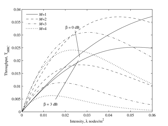
Figure 1: Throughput vs intensity of slotted ALOHA with spatial multiplexing and MRC receivers, and with $N=4$, $\alpha=3.1$, ${r_{\rm tr}}=2$ m, $\rho=25$ dB and $p=1$.

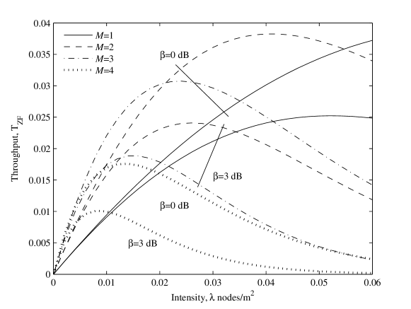
Figure 2: Throughput vs intensity of slotted ALOHA with spatial multiplexing and ZF receivers, and with $N=4$, $\alpha=3.1$, ${r_{\rm tr}}=2$ m, $\rho=25$ dB and $p=1$.

III-A1 Special Case: Spatial Multiplexing with ZF ($M=N$)

For this special case, as evident from (40), the exact outage probability and throughput expressions reduce to very simple forms, and we can gain some interesting analytical insights. In particular, taking the derivative of ${\rm T}_{\rm ZF}$, we find that with all other parameters fixed, the throughput is maximized if $\lambda$ is chosen to satisfy:

$$\lambda^{\rm opt}=\frac{\Gamma(N)}{\pi p\Gamma\left(N+\frac{2}{\alpha}\right)\Gamma\left(1-\frac{2}{\alpha}\right)\beta^{\frac{2}{\alpha}}r_{\rm tr}^{2}}\;.$$ (41)

This point is analogous to the “peaks” identified in Figs. 1 and 2, and gives the optimal tradeoff in terms of network interference and spatial multiplexing gain. As we may expect, we see that this optimal spatial intensity decreases when $N$ increases (since there is more network interference, whilst the per-link multiplexing gain is unchanged), or when $\beta$ or $r_{\rm tr}$ increases (since this puts higher reliability requirements on the per-link performance, whilst not changing the network interference). Note also that the probability of successful transmission, $1-{\rm F}_{\gamma_{\rm ZF}}(\beta)$, obtained by using $\lambda^{\rm opt}$, is $e^{-1}$. This is interesting since it coincides precisely with the probability of successful transmission for single antenna systems, presented in [25, 6].

In addition to considering the optimal $\lambda$, it is also of interest to study the optimal number of antennas. In particular, if all other parameters are kept fixed, then we find that the throughput is maximized by choosing $N$ as

$$N^{\rm opt}=\max(\lfloor x\rfloor,1)$$ (42)

with $x$ the solution to

$$\frac{\ln\left(1+\frac{1}{x}\right)\Gamma(x+1)}{\Gamma\left(x+\frac{2}{\alpha}\right)}=\frac{2\pi p\lambda\Gamma\left(1-\frac{2}{\alpha}\right)\beta^{\frac{2}{\alpha}}r_{\rm tr}^{2}}{\alpha}+\frac{\beta r_{\rm tr}^{\alpha}}{\rho}\;.$$ (43)

This is illustrated in Figs. 3, which plots the optimal number of antennas for different node intensities. We see that $N^{\rm opt}$ is decreasing in $\lambda$, in line with the observations in Figs. 1 and 2.

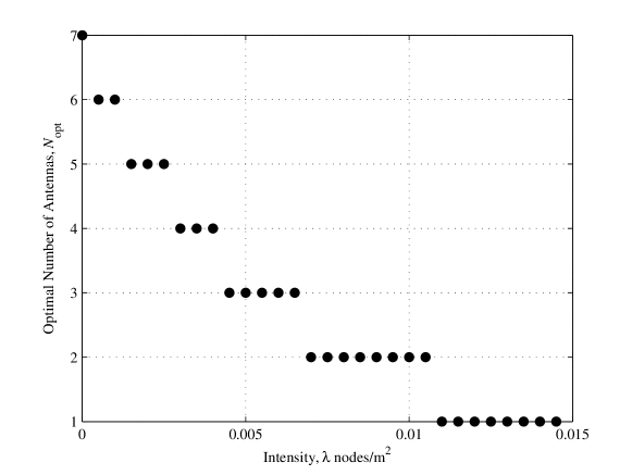
Figure 3: Optimal number of antennas vs. intensity with ${r_{\rm tr}}=3$ m, $\rho=25$ dB, $\beta=0$ dB, $\alpha=4$ and $p=1$.

III-B Throughput of OSTBC

To compute the throughput achieved by OSTBC, we substitute the relevant parameters from Table I into (1), and substitute the resulting expression into (33). Recall that the parameters from Table I give approximations for the outage probability and throughput of OSTBC, rather than exact results.

Figs. 4, 5, and 6 plot the outage probability vs. SINR threshold for three different OSTBC codes, with $N=M$. Fig. 4 is based on the code

$$\mathbf{X}_{\ell}=\left[\begin{array}[]{cccc}x_{\ell,1}&-x_{\ell,2}^{*}&x_{\ell,3}^{*}&0\\ x_{\ell,2}&x_{\ell,1}^{*}&0&x_{\ell,3}^{*}\\ x_{\ell,3}&0&-x_{\ell,1}^{*}&-x_{\ell,2}^{*}\\ 0&x_{\ell,3}&x_{\ell,2}&-x_{\ell,1}\end{array}\right]\;,$$ (44)

Fig. 5 is based on the code

$$\mathbf{X}_{\ell}=\left[\begin{array}[]{cccc}x_{\ell,1}&0&x_{\ell,2}&-x_{\ell,3}\\ 0&x_{\ell,1}&x_{\ell,3}^{*}&x_{\ell,2}^{*}\\ -x_{\ell,2}^{*}&-x_{\ell,3}&x_{\ell,1}^{*}&0\end{array}\right]\;,$$ (45)

and Fig. 6 is based on the code

$$\mathbf{X}_{\ell}=\left[\begin{array}[]{cccc}x_{\ell,1}&-x_{\ell,2}^{*}&0&0\\ x_{\ell,2}&x_{\ell,1}^{*}&0&0\\ 0&0&x_{\ell,1}&-x_{\ell,2}^{*}\\ 0&0&x_{\ell,2}&x_{\ell,1}^{*}\end{array}\right]\;.$$ (46)

The analytical curves are seen to accurately approximate the Monte Carlo simulated curves for all SINR thresholds. For further comparison, the outage probability approximation given in [12] is also shown. The increased accuracy of our approximation is clearly evident.

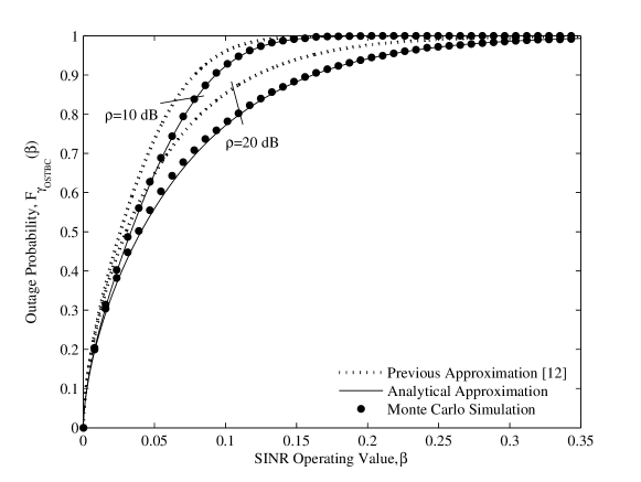
Figure 4: Outage probability vs SINR of slotted ALOHA with OSTBC using the code in (44), and with $\alpha=3.5$, ${r_{\rm tr}}=5$ m, $\lambda=0.1$ nodes/${\rm m}^{2}$, $N=4$ and $p=1$.

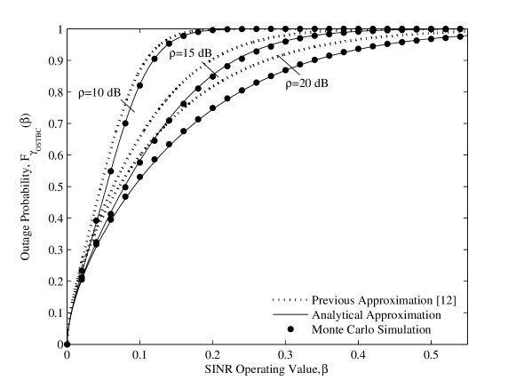
Figure 5: Outage probability vs SINR of slotted ALOHA with OSTBC using the code in (45), and with $\alpha=3.5$, ${r_{\rm tr}}=5$ m, $\lambda=0.05$ nodes/${\rm m}^{2}$, $N=3$ and $p=1$.

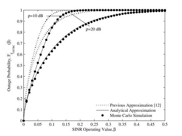
Figure 6: Outage probability vs SINR of slotted ALOHA with OSTBC using the code in (46), and with $\alpha=3.5$, ${r_{\rm tr}}=5$ m, $\lambda=0.1$ nodes/${\rm m}^{2}$, $N=4$ and $p=1$.

Note that our outage probability approximation becomes an exact result for the important class of cyclic antenna diversity codes, which transmit only one symbol per OSTBC codeword, with the symbol being sent out of a different antenna during each channel use. For example, for the case $M=4$, the codeword matrix $\mathbf{X}_{\ell}$ for this coding scheme would have the form

$$\mathbf{X}_{\ell}=x_{\ell,1}\mathbf{I}_{4}\;.$$ (47)

This type of code, whilst achieving full spatial diversity order, results in the lowest code rate among all OSTBC codes, under the assumption that at least one symbol is transmitted per time slot. However, as we show in Section IV, if the network is sufficiently dense, then this type of coding scheme becomes optimal in terms of maximizing throughput, due to the minimal network interference it yields compared with other higher rate codes.

Fig. 7 shows the throughput achieved by OSTBC, based on (33), for different SINR operating values $\beta$, and different numbers of antennas used for transmission $M$. The codes used for $M=2$ and $M=3$ are given by (24) and (45) respectively. Note that both of these codes correspond to maximum-rate codes for the particular antenna configuration employed [22]. As with spatial multiplexing, we see that for all curves, the throughput increases monotonically with $\lambda$ up to a certain peak point, after which the throughput decreases monotonically.

Fig. 7 also reveals the interesting fact that the throughput can be significantly higher if less antennas are used for transmission. This can be explained by first noting that for $M=2$ when using the code in (24), we have $\frac{N_{I}}{M}=2$, and for $M=3$ when using the code in (45), we have $\frac{N_{I}}{M}=\frac{7}{3}$ . Hence, whilst increasing $M$ increases the spatial diversity order, it also increases $\frac{N_{I}}{M}$. (Note that for maximum-rate codes, such as the ones used in Fig. 7, it can easily be shown that $N_{I}$ is always an increasing function of $M$.) Further, by invoking Lemma 4, we see that the moments of the approximate normalized interference term $\tilde{\mathcal{K}}_{\ell}$ in (30) are increasing functions of $\frac{N_{I}}{M}$. This suggests that the additional interference in the network caused by each transmitting node employing $M=3$ antennas using the code in (45), compared with $M=2$ antennas using the code in (24), outweighs the benefits in terms of an increased spatial diversity order.

Fig. 8 shows the throughput achieved by OSTBC, based on (33), for different SINR operating values $\beta$, and different values of $N_{I}$. In particular, for $N_{I}=4$, $N_{I}=8$, and $N_{I}=12$, we use the codes in (47), (46), and (44) respectively. Note that each of these codes have the same diversity order, but different code rates $R$. Specifically, for the case $N_{I}=4$, $R=\frac{1}{4}$; for the case $N_{I}=8$, $R=\frac{1}{2}$; and for the case $N_{I}=12$, $R=\frac{3}{4}$. Clearly the code rate is an increasing function of $N_{I}$. Fig. 8 reveals the interesting fact that in many cases, the throughput is higher when a lower code rate is used. This is because the additional interference caused by more simultaneous symbol transmissions in the network outweighs the benefits of an increased code rate.

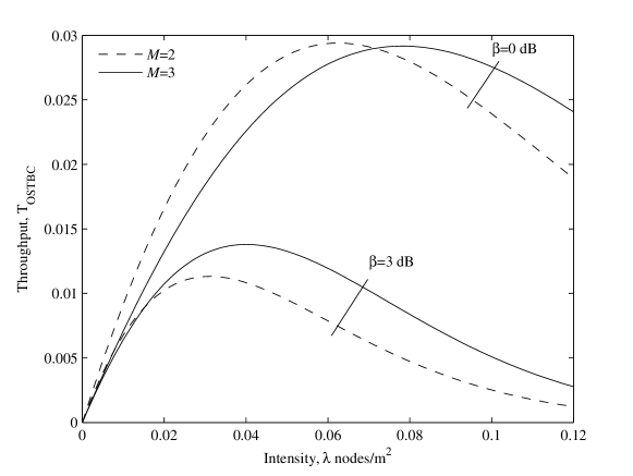
Figure 7: Throughput vs intensity of slotted ALOHA with OSTBC, and with $N=4$, $\alpha=3.1$, ${r_{\rm tr}}=2$ m, $\rho=25$ dB and $p=1$.

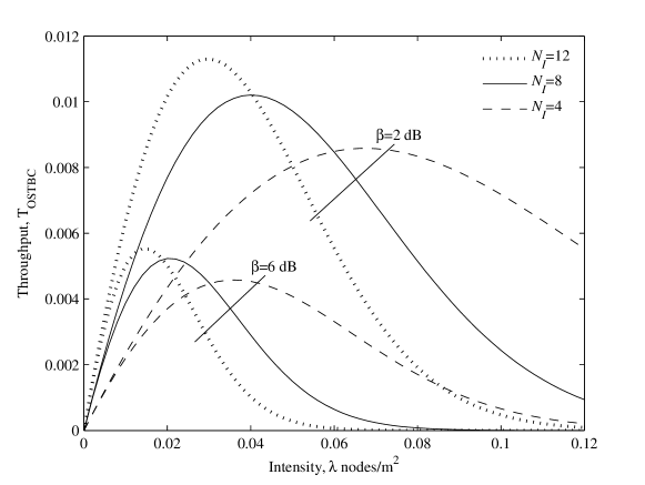
Figure 8: Throughput vs intensity of slotted ALOHA with OSTBC, and with $N=4$, $\alpha=3.1$, ${r_{\rm tr}}=3$ m, $\rho=20$ dB and $p=1$.

III-C Comparison

We see in Table I that the signal and interference powers for the spatial multiplexing and OSTBC schemes are different, and are dependent on the system parameters $M$, $N$, $R$ and $N_{I}$. As such, it is not straightforward to determine which scheme performs the best, and under which scenario. For example, when $M=2$, it can be shown that the signal power of OSTBC using the Alamouti code is greater than spatial multiplexing with ZF receivers, while the interference power of both OSTBC and spatial multiplexing schemes are the same. However, for a fixed $\beta$, the per-link data rate for spatial multiplexing is twice that of OSTBC, due to the $M=2$ transmitted streams per node for spatial multiplexing. Thus although the SINR of OSTBC is greater than spatial multiplexing with ZF receivers for $M=2$, the overall network throughput may not be greater.

The best performing receiver used for spatial multiplexing is also dependent on the particular scenario. For example, it is well known that for a single user MIMO system with no interfering nodes, spatial multiplexing with ZF receivers performs better than spatial multiplexing with MRC receivers at high SNR, hence ZF receivers is expected to perform better than MRC receivers in sparse networks. However, for MRC receivers, as the node density increases, the impact of the interference from other transmitting nodes becomes more dominant than the self-interference. By noting that the distribution of the interference power from these interfering transmitting nodes for both MRC and ZF receivers are equal, the distribution of the total interference for both MRC and ZF receivers thus converge with increasing node density. The key factor which distinguishes between these two schemes in dense networks is the signal power, which is greater for MRC receivers. This suggests that the best performing receiver used for spatial multiplexing is dependent on the particular node density.

The preceding discussion suggests that the best performing scheme is dependent on the system and network parameters. This can be seen in Fig. 9, which plots the network throughput vs. node intensity $\lambda$, of spatial multiplexing with MRC and ZF receivers, and OSTBC, based on (33), for different numbers of antennas used for transmission, $M$. We observe that spatial multiplexing with ZF performs the best in sparse network configurations (i.e., small $\lambda$), while OSTBC performs the best in dense networks (i.e., high $\lambda$). Further, spatial multiplexing with MRC receivers is seen to perform better than ZF receivers at high $\lambda$, which agrees with previous discussion. We will also prove this analytically in Section IV.

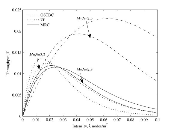
Figure 9: Throughput vs intensity of slotted ALOHA with spatial multiplexing and OSTBC, and with $\alpha=3.3$, ${r_{\rm tr}}=2$ m, $\rho=25$ dB, $\beta=2$ dB and $p=1$.

The best performing scheme can also be shown to be dependent on the SINR $\beta$ operating value, as shown in Fig. 10, which plots the network throughput vs. SINR $\beta$ for all three schemes, again for different $M$. We see that spatial multiplexing with MRC receivers performs the best for low $\beta$, while OSTBC performs the best for high $\beta$.

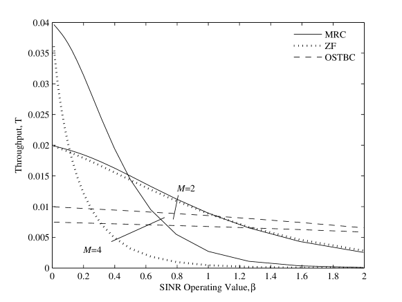
Figure 10: Throughput vs SINR operating value $\beta$ of slotted ALOHA with spatial multiplexing and OSTBC, and with $N=4$, $\alpha=2.5$, ${r_{\rm tr}}=3$ m, $\rho=20$ dB, $\lambda=0.01$ nodes/${\rm m}^{2}$ and $p=1$.

As can be seen from Figs. 1–10, the impact of the number of antennas used for transmission, and the relative throughput of the spatial multiplexing and OSTBC systems are dependent on different network parameters. To explore this further, it is convenient to analyze the throughput of spatial multiplexing and OSTBC in asymptotic regimes. This is considered in the following section.

IV Network Throughput: Asymptotic Analysis

In this section, we analyze the performance of spatial multiplexing and OSTBC in dense networks, and for low and high $\beta$ operating values. We note that in sparse networks, the performance of spatial multiplexing and OSTBC approaches the performance of single user MIMO systems, for which the performance is well known (see e.g., [1, 2, 3, 4]). Thus, although we investigate dense network scenarios, we do not consider the opposite case of sparse networks in this paper. Note also, that for $M=1$, corresponding to single-input multiple-output (SIMO) transmission, the performance of all schemes are the same.

IV-A Dense Networks (Large $\lambda$)

Under dense network conditions, we have the following corollary.

Corollary 2

As $\lambda\to\infty$, the SINR c.d.f. in (1) behaves as

$${\rm F}_{\gamma}(\beta)={\rm F}_{\gamma,\lambda\to\infty}(\beta)+o\left(e^{-\lambda\left(\frac{\beta\Omega}{\theta}\right)^{\frac{2}{\alpha}}\eta(n)}\lambda^{m-1}\right)$$ (48)

where

$${\rm F}_{\gamma,\lambda\to\infty}(\beta)=1-\frac{2\eta(n)}{\alpha\Gamma(m)}\left(\frac{\beta\Omega}{\theta}\right)^{\frac{2}{\alpha}}{\rm E}_{Y}\left[e^{-\frac{\beta Y}{\theta}}\right]e^{-\frac{\beta}{\theta}}e^{-\lambda\left(\frac{\beta\Omega}{\theta}\right)^{\frac{2}{\alpha}}\eta(n)}\lambda^{m-1}$$

and

$${\rm E}_{Y}\left[e^{-\frac{\beta Y}{\theta}}\right] =\left(\frac{\theta}{\Upsilon\beta+\theta}\right)^{u}\;.$$ (49)

To give an indication as to when a network is “sufficiently dense” such that the expansion (2) is accurate, Table II tabulates the quantity $1/\lambda_{\rm min}$, with $\lambda_{\min}$ representing the minimum node density required such that (2) is within at least $85\%$ of the true non-asymptotic value. Intuitively, the quantity $1/\lambda_{\rm min}$ gives a measure of the maximum allowable separation between adjacent transmitting nodes (on average), in order for the asymptotic expansion (2) to serve as a good approximation. Note that a scenario with $M=1$ data streams is chosen, because as we will discuss later, single-stream transmission is throughput-optimal in dense networks. Moreover, a transmit-receive distance of $5$ ${\rm m}$ is chosen, which is practically relevant (e.g., for wireless local area networks).

TABLE II: Average maximum area around each transmitting node, such that $\frac{\biggr{|}{\rm F}_{\gamma,\lambda\to\infty}(\beta)-{\rm F}_{\gamma}(\beta)\biggr{|}}{1-{\rm F}_{\gamma}(\beta)}>0.15$, for various SINR thresholds $\beta$ and transmit SNRs $\rho$ with $M=1$, $N=3$, $r_{\rm tr}=5$ m and $\alpha=2.1$.

$\rho$ dB $\setminus\beta$ dB	$1$	$2$	$5$	$10$	$20$
$2$	6.500	6.486	6.383	6.114	5.506
$5$	12.447	12.519	12.520	12.133	10.981
$10$	33.478	34.674	36.900	37.481	34.638
$20$	111.483	130.208	193.050	286.532	335.569

The results in the table show that the large–$\lambda$ expansion (2) serves as an accurate performance measure for practical network configurations; in some cases, applying even when the networks are relatively sparse. This is particularly true for moderate to large SNRs. For example, at $10$ dB SNR, a transmitter spacing of roughly $35$ ${\rm m}^{2}$ on average is sufficient, which is relatively large compared with the transmit-receive distance of $5$ m. As the SNR is reduced, e.g., to $2$ dB, a closer transmitter spacing of roughly $6$ ${\rm m}^{2}$ is needed. This behavior is intuitive, since dense networking conditions are representative of interference-limited scenarios, in which case the interference in the network is much more significant compared with the noise. If the SNR is reduced, then the noise has greater relative effect, and there must be more interference (i.e., a greater density $\lambda$) in order for the interference-limited behavior to be apparent.

From (33) and (48), and recalling that $\Omega/\theta=r_{\rm tr}^{\alpha}$ for each scheme (c.f. Table I), it follows that for large $\lambda$ the throughput becomes

$${\rm T}\propto e^{-\lambda\beta^{\frac{2}{\alpha}}r_{\rm tr}^{2}\eta(n)}\;\lambda^{m}\;.$$ (50)

From this, we can obtain some useful insights into the network performance and optimization:

• The throughput decays exponentially in $\lambda$. This loss of throughput indicates that in dense networks, the negative effects of interference will dominate any positive throughput gains obtained by an increase in the number of communication links.

• Since the exponential in (50) dominates for large $\lambda$, the component $\eta(n)$ is a critical factor which determines performance. Moreover, since $n$ is proportional to the effective interference power caused by each interfering transmitter, and $\eta(n)$ increases with $n$, for all three transmission schemes it is best to choose $n$ as small as possible. Thus, recalling the parameters in Table I, we have the following design criteria for dense networks:

  • For spatial multiplexing with either MRC or ZF receivers, it is optimal to use only a single transmit stream (i.e., $M=1$).

  • For OSTBC, it is optimal to use a cyclic antenna diversity coding scheme. This code, illustrated in (47) for $M=4$, minimizes $n$ by maximizing the coding parameter $N_{I}$ (i.e., $N_{I}=M$). To determine the optimal $M$ for cyclic antenna diversity codes, we consider the leading order factor $\lambda^{m}$. As $m$ is proportional to the spatial diversity order, we note that the optimal choice is $M=N$.

• For systems with $M>1$, OSTBC codes with $N_{I}<M^{2}$ will yield a higher throughput than both spatial multiplexing schemes; whereas, if $N_{I}>M^{2}$, the throughput will be worse than both. This can be seen by again noting that the exponential in (50) dominates for large $\lambda$. As $N_{I}=M$ for cyclic antenna diversity code, we see that these codes always perform better than spatial multiplexing. For the remaining case $N_{I}=M^{2}$, which only occurs for the Alamouti code and therefore $M=2$, the throughputs of all three schemes have the same exponential decay in (50); however, OSTBC has the largest leading order factor $\lambda^{m}$, and therefore achieves the highest throughput. Finally, for all $M>1$, spatial multiplexing with MRC achieves a higher throughput than ZF.

In general, these results reveal that OSTBC with a $M=N$ cyclic antenna diversity code is the optimal scheme in dense networks.

IV-B Networks with High SINR Operating Values (Large $\beta$)

For networks with high SINR operating values, we have the following corollary.

Corollary 3

As $\beta\to\infty$, the SINR c.d.f. (1) behaves as

$${\rm F}_{\gamma}(\beta) ={\rm F}_{\gamma,\beta\to\infty}(\beta)+o\left({\rm E}_{Y}\left[e^{-\frac{\beta Y}{\theta}}\right]e^{-\frac{\beta}{\theta}}e^{-\lambda\left(\frac{\beta\Omega}{\theta}\right)^{\frac{2}{\alpha}}\eta(n)}\beta^{m-1}\right)$$ (51)

where

$${\rm F}_{\gamma,\beta\to\infty}(\beta)=1-\frac{1}{\Gamma(m)\theta^{m-1}}{\rm E}_{Y}\left[e^{-\frac{\beta Y}{\theta}}\right]e^{-\frac{\beta}{\theta}}e^{-\lambda\left(\frac{\beta\Omega}{\theta}\right)^{\frac{2}{\alpha}}\eta(n)}\beta^{m-1}\;.$$ (52)

To check the accuracy of this expansion, Table III tabulates for various scenarios the minimum SINR operating value $\beta$ such that (52) is within $85\%$ of the true non-asymptotic value. These results demonstrate that the large–$\beta$ expansion (52) serves as an accurate performance measure for practical network configurations; in some cases, applying even when $\beta$ is low. This is particularly true for low to moderate SNRs. For example, at $2$ dB SNR and $\lambda$ chosen such that the average transmitter spacing is $20$ ${\rm m}^{2}$, a SINR operating value of $-12.832$ dB or above is sufficient—something which is expected to be true for most wireless applications. As the SNR is increased, e.g., to $10$ dB, a higher SINR operating value of $-1.726$ dB or above is needed. This matches with intuition, since, if the network is relatively sparse (as in the example above), then for the outage probability to remain constant as the SINR is increased, the SNR must increase accordingly.

TABLE III: Minimum SINR $\beta$ (dB) operating value such that $\frac{\biggr{|}{\rm F}_{\gamma,\beta\to\infty}(\beta)-{\rm F}_{\gamma}(\beta)\biggr{|}}{1-{\rm F}_{\gamma}(\beta)}>0.15$, for various $1/\lambda$, and transmit SNRs $\rho$ with $M=1$, $N=3$, $r_{\rm tr}=5$ m and $\alpha=4$.

$\rho$ dB $\setminus\frac{1}{\lambda}{\rm m}^{2}$	$100$	$50$	$20$	$12.5$	$10$
$2$	-14.547	-14.078	-12.832	-11.543	-10.701
$5$	-11.421	-10.804	-8.925	-7.211	-6.142
$10$	-5.933	-4.827	-1.726	0.885	2.366
$15$	-0.078	1.833	6.569	9.948	11.699

From (33) and (51), and recalling that $\Omega/\theta=r_{\rm tr}^{\alpha}$ for each scheme (c.f. Table I), it follows that for large $\beta$ the throughput becomes

$${\rm T}\propto\frac{1}{\Gamma(m)\theta^{m-1}\Upsilon^{u}}e^{-\frac{\beta}{\theta}}e^{-\lambda r_{\rm tr}^{2}\beta^{\frac{2}{\alpha}}\eta(n)}\beta^{m-1-u}\;.$$ (53)

From this, we can obtain some useful insights into the network performance and optimization:

• Recalling that $\alpha>2$, we see that the exponential $e^{-\frac{\beta}{\theta}}$ in (53) dominates for large $\beta$. This is intuitive, by recalling the direct correspondence between the SINR operating value $\beta$ and the outage probability.

• The component $\theta$, which represents the transmit SNR, is a critical factor, and this quantity should be maximized in order to maximize the throughput. When $\theta$ is independent of $M$, as is the case for cyclic antenna diversity codes, the $\beta^{m-1-u}$ polynomial term should be maximized in order to maximize the throughput. Recalling the parameters from Table I, we arrive at the following design criteria for networks with high SINR operating values:

  • The optimal transmission scheme is the same as for dense networks. That is, for spatial multiplexing with either MRC or ZF receivers it is optimal to use only a single transmit stream, whereas for OSTBC it is optimal to use the $M=N$ cyclic antenna diversity coding scheme.

  Note that if the SNR is also sufficiently high, then the exponential $e^{-\lambda r_{\rm tr}^{2}\beta^{\frac{2}{\alpha}}\eta(n)}$ may dominate $e^{-\frac{\beta}{\theta}}$; however, it is easy to see that the same optimality criteria still applies.

• For systems with $M>1$, OSTBC codes yield a higher throughput than each of the spatial multiplexing schemes. Moreover, since the throughput of both spatial multiplexing schemes have the same exponential decay and also the same polynomial factor $\beta^{m-1-u}$ in (53), their relative performance is determined by the constant factor $\frac{1}{\Gamma(m)\theta^{m-1}\Upsilon^{u}}$. Thus, by substituting the relevant parameters from Table I, we can show that ZF will deliver a higher throughput than MRC if the following condition is met:

  $$\rho\geq Mr_{\rm tr}^{\alpha}\left(\frac{\Gamma(N-M+1)}{\Gamma(N)}\right)^{\frac{1}{M-1}},$$ (54)

  otherwise MRC will perform better.

In general, these results indicate that, as for dense networks, OSTBC with a $M=N$ cyclic antenna diversity code is the preferable scheme for high SINR operating values.

IV-C Networks with Low SINR Operating Values (Small $\beta$)

For networks with low SINR operating values, we have the following corollary.

Corollary 4

As $\beta\to 0^{+}$, the SINR c.d.f. (1) behaves as

$${\rm F}_{\gamma}(\beta) ={\rm F}_{\gamma,\beta\to 0^{+}}(\beta)+O\left(\beta\right)$$ (55)

where

$${\rm F}_{\gamma,\beta\to 0^{+}}(\beta)=\lambda\frac{\Gamma\left(m-\frac{2}{\alpha}\right)}{\Gamma(m)}\frac{\eta(n)}{\Gamma\left(1-\frac{2}{\alpha}\right)}\left(\frac{\beta\Omega}{\theta}\right)^{\frac{2}{\alpha}}\;.$$ (56)

To give an indication of when the expansion (56) is accurate, Table IV tabulates the maximum SINR operating values such that (56) is within $85\%$ of the true non-asymptotic value. From the table, we see that quite low SINR operating values are required, and these may or may not be practical. Nevertheless, as we discuss shortly, the insights we will obtain from (56) also turn out to be valid for much higher SINR operating values than those tabulated in Table IV.

TABLE IV: Maximum SINR $\beta$ (dB) operating value such that $\frac{\biggr{|}{\rm F}_{\gamma,\beta\to 0^{+}}(\beta)-{\rm F}_{\gamma}(\beta)\biggr{|}}{1-{\rm F}_{\gamma}(\beta)}>0.15$, for various $1/\lambda$ and transmit SNRs $\rho$. Spatial multiplexing with MRC receivers is considered with $M=4$, $N=4$, $r_{\rm tr}=5$ m and $\alpha=3$.

$\rho$ dB $\setminus\frac{1}{\lambda}{\rm m}^{2}$	$100$	$50$	$20$	$12.5$	$10$
$10$	-22.055	-22.660	-24.559	-27.033	-30.362
$15$	-18.164	-19.462	-22.518	-25.850	-29.788
$20$	-15.476	-17.467	-21.487	-25.346	-29.586
$25$	-14.0351	-16.501	-21.068	-25.171	-29.547
$30$	-13.435	-16.128	-20.921	-25.100	-29.508

From (33) and (55), and recalling that $\Omega/\theta=r_{\rm tr}^{\alpha}$ for each scheme (c.f. Table I), it follows that for small $\beta$ the throughput becomes

$${\rm T}\propto\zeta p\lambda\left(1-\frac{\Gamma\left(m-\frac{2}{\alpha}\right)}{\Gamma(m)}\frac{\eta(n)}{\Gamma\left(1-\frac{2}{\alpha}\right)}\lambda r_{\rm tr}^{2}\beta^{\frac{2}{\alpha}}\right)\;.$$ (57)

From the preceding equations, we can obtain the following useful insights:

• If $\beta$ is “very” small (i.e., such that the $\beta$-dependent term in (57) is negligible), then the throughput approaches $\zeta\lambda p$, which trivially gives the following design criteria:

  • For spatial multiplexing with either MRC or ZF receivers, it is optimal to use the maximum number of transmit streams.

  • For OSTBC, it is optimal to use maximum-rate codes. This follows by noting that the maximum code rate is a decreasing function of the number of antennas used for transmission when $M\geq 2$ [22], and thus increasing the number of antennas for transmission leads to a lower throughput. The codes with the maximum-rate corresponds to either SIMO transmission with $M=1$ or the Alamouti code with $M=2$. From (55), the Alamouti code performs better than SIMO if

    $$\frac{\Gamma\left(N-\frac{2}{\alpha}\right)\Gamma(2N)}{\Gamma(N)\Gamma\left(2N-\frac{2}{\alpha}\right)}>\left(1+\frac{2}{\alpha}\right)\;.$$ (58)

    We observe that this occurs for low path loss exponents, i.e., as $\alpha\to 2$.

  Intuitively, the outage probability is very close to zero, and therefore it makes sense to send as much information as possible during each channel use. For this scenario, spatial multiplexing thus performs better than OSTBC.

• More generally, for all $\beta$ values for which (57) is accurate (i.e., the $\beta$-dependent term in (57) is not necessarily negligible), we can derive the following conditions:

  • For spatial multiplexing with MRC and ZF receivers, the optimal number of data streams is given by

    $$M^{\rm opt}=\min\left(\max\left(\lfloor x\rfloor,1\right),N\right)\,$$ (59)

    where, for MRC, $x$ is the solution to

    $$\frac{1}{\lambda\pi pr_{\rm tr}^{4}\beta^{\frac{2}{\alpha}}} =\frac{\Gamma\left(N-\frac{2}{\alpha}\right)}{\Gamma(N)}{\frac{\Gamma\left(x-1+\frac{2}{\alpha}\right)}{\Gamma(x-1)}}\left(1+\frac{2x}{\alpha(x-1)}\right)\;,$$ (60)

    whilst, for ZF, it is the solution to

    $$\frac{1}{\lambda\pi pr_{\rm tr}^{4}\beta^{\frac{2}{\alpha}}}=\frac{\Gamma\left(N-x+1-\frac{2}{\alpha}\right)}{\Gamma(N-x+1)}{\frac{\Gamma\left(x-1+\frac{2}{\alpha}\right)}{\Gamma(x-1)}}\left(1+\frac{2x}{\alpha(x-1)}+\frac{2(x-1)}{\alpha(N-x+1)}\right)\;.$$ (61)

    Note that the right hand sides of both (60) and (61) are increasing in $x$, hence $M_{\rm opt}$ is unique.

  • As $N\to\infty$,

    $$\frac{M_{\rm opt}}{N}\to\varrho^{\rm opt}$$ (62)

    where, for MRC,

    $$\varrho^{\rm opt}=\frac{1}{\beta}\left(\frac{\alpha}{\lambda\pi pr_{\rm tr}^{4}(\alpha+2)}\right)^{\frac{\alpha}{2}}\;,$$ (63)

    whist, for ZF, $\varrho^{\rm opt}$ is the solution to

    $$\varrho^{\rm opt} =\frac{\frac{1}{\beta}\left(\frac{\alpha}{\lambda\pi pr_{\rm tr}^{4}(\alpha+2)}\right)^{\frac{\alpha}{2}}\left(1-\varrho^{\rm opt}\right)}{\left(1+\left(\frac{\varrho^{\rm opt}}{1-\varrho^{\rm opt}}\right)\left(\frac{2}{\alpha+2}\right)\right)^{\frac{\alpha}{2}}}\;.$$ (64)

  These equations confirm the intuition that, for both receivers, as the node density is increased, less transmit antennas should be used. This is because adding more nodes to the network increases the aggregate interference, and thus, it is better for each node to transmit will less data streams in order to “balance” the overall network interference. This behavior was also observed for SINR operating values as high as $3$ dB in Figs. 1 and 2.

• The results above also reveal that less transmit antennas should be used if the SINR operating value $\beta$ increases, a phenomenon which is confirmed in Fig. 10. Moreover, the optimal number of transmit antennas is at least as many for MRC as for ZF. For the example shown in Fig. 10, for MRC, all transmit antennas should be used when $\beta$ is below $-3$ dB; whereas for ZF, $\beta$ must be below $-10$ dB.

• By noting that $R(M)<1$, it is clear that spatial multiplexing performs better than OSTBC. Moreover, for spatial multiplexing, since $\frac{\Gamma\left(m-\frac{2}{\alpha}\right)}{\Gamma(m)}$ is decreasing in $m$, for $M>2$, MRC achieves a higher throughput than ZF.

In general, these results indicate that spatial multiplexing with MRC, with all transmit antennas active, is the most favorable scheme for low SINR operating values.

V Transmission Capacity

In this section, we turn to the analysis of transmission capacity. In general, we find that for both spatial multiplexing and OSTBC, an exact analysis of the transmission capacity is intractable due to the complexity involved with inverting the exact outage probability expressions. One exception is the case of spatial multiplexing with ZF receivers with $M=N$, for which an exact expression for the transmission capacity is obtained from (40) and (34) as

$${\rm c}_{\rm ZF}(\epsilon)=\frac{N(1-\epsilon)}{(\beta R^{\alpha})^{\frac{2}{\alpha}}\eta(N)}\left(\log\left(\frac{1}{1-\epsilon}\right)-\frac{\beta r_{\rm tr}^{\alpha}N}{\rho}\right)\;.$$ (65)

For all other scenarios, we focus on studying the transmission capacity for small outage levels, which is representative of practical systems. Under these conditions, based on (35), we present the following key theorem which, after substituting the parameters in Table I, yields closed-form expressions for the transmission capacity of the spatial multiplexing and OSTBC schemes.

Theorem 2

If the SINR takes the general form in (35), then the transmission capacity as $\epsilon-{\rm F}^{\rm SU}(\beta)\to 0$ can be written as

$${\rm c}(\epsilon) =\frac{\zeta\theta^{\frac{2}{\alpha}}\Gamma(n)\Gamma(m)}{\pi\beta^{\frac{2}{\alpha}}\Omega^{\frac{2}{\alpha}}\Gamma\left(n+\frac{2}{\alpha}\right)\Gamma\left(m-\frac{2}{\alpha}\right)}\frac{\left(\epsilon-{\rm F}^{\rm SU}(\beta)\right)^{+}}{{\rm E}_{Y}\left[e^{-\frac{\beta(Y+1)}{\theta}}{}_{1}F_{1}\left(1-m,1+\frac{2}{\alpha}-m,\frac{\beta(Y+1)}{\theta}\right)\right]}+O\left(\left(\left(\epsilon-{\rm F}^{\rm SU}(\beta)\right)^{2}\right)^{+}\right)$$ (66)

where ${}_{1}F_{1}(\cdot,\cdot,\cdot)$ is the Kummer confluent hypergeometric function, and the notation $(\cdot)^{+}$ implies $(a)^{+}=\max(a,0)$. Also, the expectation in (66) can be written as

$${\rm E}_{Y}[\cdots] =\frac{e^{-\frac{\beta}{\theta}}}{\Gamma\left(m-\frac{2}{\alpha}\right)}\sum_{\ell=0}^{m-1}\binom{m-1}{\ell}\left(\frac{\beta}{\theta}\right)^{\ell}\Gamma\left(m-\ell-\frac{2}{\alpha}\right)\sum_{\tau=0}^{\ell}\binom{\ell}{\tau}{\rm E}_{Y}\left[e^{-\frac{\beta Y}{\theta}}Y^{\tau}\right],$$ (67)

and ${\rm F}^{\rm SU}(\beta)$ represents the outage probability with no multi-node interference, computed as

$${\rm F}^{\rm SU}(\beta)={\rm Pr}\left(\frac{W}{Y+1}\leq\beta\right)=1-e^{-\frac{\beta}{\theta}}\sum_{k=0}^{m-1}\frac{\left(\frac{\beta}{\theta}\right)^{k}}{k!}\sum_{\tau=0}^{k}\binom{k}{\tau}{\rm E}_{Y}\left[e^{-\frac{\beta Y}{\theta}}Y^{\tau}\right]\;.$$ (68)

The remaining expectations are given in closed-form in (39).

Proof:

Follows by taking a Taylor expansion of (1) around $\lambda=0$, and then finding the inverse of the resulting expression w.r.t. $\lambda p$. ∎

Note that the factor ${\rm F}^{\rm SU}(\beta)$ represents the outage probability of a single user MIMO system, for which outages are caused by self-interference and AWGN. Due to the additional multi-node interference in ad hoc networks, any specified outage constraint $\epsilon$ which falls below ${\rm F}^{\rm SU}(\beta)$ can never be met, and therefore the transmission capacity in such cases is zero. This phenomenon is illustrated in Fig. 11, where the outage probability is plotted versus intensity for spatial multiplexing with MRC receivers, for different antenna configurations. For the results shown, an outage probability of less than $0.2$ can never be achieved when $M\geq 2$, due to the effects of AWGN and self-interference, which ensures that $\epsilon>0$ when $\lambda=0$. Note however, that for OSTBC and spatial multiplexing with ZF receivers, there is no self-interference, and ${\rm F}^{\rm SU}(\beta)$ in this case accounts for outages due to AWGN only.

Figure 11: Outage probability vs. intensity of slotted ALOHA with spatial multiplexing using MRC receivers, and with $N=4$, ${r_{\rm tr}}=3$ m, $\alpha=4.23$, $\beta=3$ dB, $\rho=30$ dB and $p=1$.

To compute the transmission capacity achieved by spatial multiplexing and OSTBC, we substitute the relevant parameters from Table I into (66). The accuracy of our transmission capacity expression is confirmed in Fig. 12, which plots the transmission capacity vs. outage probability $\epsilon$ for spatial multiplexing with ZF receivers. We see that for outage probabilities as high as $\epsilon=0.1$, our expression is accurate. Although not shown, similar accuracy has been observed for the other schemes also.

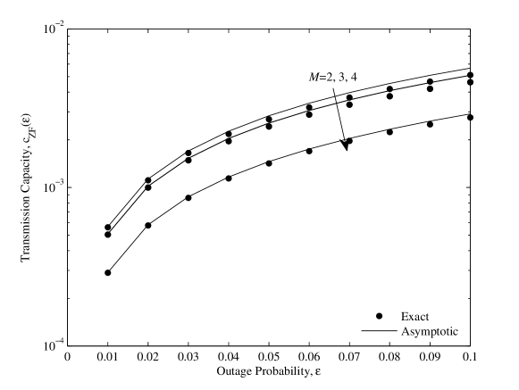
Figure 12: Transmission capacity vs. outage probability of slotted ALOHA using ZF receivers, and with ${r_{\rm tr}}=3$ m, $\beta=3$ dB, $\alpha=4$, $N=4$ and $p=1$.

For large numbers of antennas, we present the following corollary for the transmission capacity.

Corollary 5

As $M,N\to\infty$, the transmission capacity as $\epsilon-{\rm F}^{\rm SU}(\beta)\to 0$ satisfies

$$\frac{{\rm c}(\epsilon)}{\zeta} =\left(\frac{\left(m\theta-\beta-\beta u\Upsilon\right)^{+}}{n\Omega}\right)^{\frac{2}{\alpha}}\frac{\left(\epsilon-{\rm F}^{\rm SU}(\beta)\right)^{+}}{{\pi r_{\rm tr}^{2}\beta^{\frac{2}{\alpha}}}}+O\left(\left(\left(\epsilon-{\rm F}^{\rm SU}(\beta)\right)^{2}\right)^{+}\right)\;.$$ (69)

Proof:

See Appendix -C. ∎

(69) implies that if $\epsilon>{\rm F}^{\rm SU}(\beta)$ and $\frac{\left(m\theta-\beta-\beta Y\right)^{+}}{n\Omega}$ converges to a constant for large $M,N$, then the transmission capacity will scale linearly with $\zeta$. In the following, we will use these results to investigate how the transmission capacity scales with the number of antennas, for the spatial multiplexing and OSTBC systems which we consider. Under some conditions, we will show that linear scaling is indeed possible.

V-A Transmission Capacity of Spatial Multiplexing

Here we use Corollary 5 to gain insights into the scaling behavior of the transmission capacity for spatial multiplexing with MRC and ZF receivers, as given by the following corollaries.

Corollary 6

As $N\to\infty$ with $M=\kappa N$ where $0<\kappa\leq 1$, the transmission capacity of spatial multiplexing with MRC receivers as $\epsilon-H\left(\beta-\bar{\beta}_{\rm MRC}\right)\to 0$ behaves as

$$\frac{{\rm c}_{\rm MRC}(\epsilon)}{N}\to\kappa\left(\frac{r_{\rm tr}^{\alpha}}{\rho}+1\right)^{\frac{2}{\alpha}}\left(\left(\bar{\beta}_{\rm MRC}-\beta\right)^{+}\right)^{\frac{2}{\alpha}}\frac{\left(\epsilon-H\left(\beta-\bar{\beta}_{\rm MRC}\right)\right)^{+}}{\pi r_{\rm tr}^{2}\beta^{\frac{2}{\alpha}}}+O\left(\left(\left(\epsilon-H\left(\beta-\bar{\beta}_{\rm MRC}\right)\right)^{2}\right)^{+}\right)$$ (70)

where

$$\bar{\beta}_{\rm MRC}=\frac{1}{\kappa\left(\frac{r_{\rm tr}^{\alpha}}{\rho}+1\right)}$$ (71)

and $H(\cdot)$ is the Heaviside step function.

Proof:

Follows by substituting the relevant parameters for MRC receivers in Table I into (69), and noting that [26, Eq. (8)] $\frac{W}{Y+1}$ converges in probability to $\frac{1}{\kappa\left(\frac{r_{\rm tr}^{\alpha}}{\rho}+1\right)}$ as $N\to\infty$ with $M=\kappa N$. ∎

Corollary 7

As $N\to\infty$ with $M=\kappa N$ where $0<\kappa<1$, the transmission capacity of spatial multiplexing with ZF receivers as $\epsilon-H\left(\beta-\bar{\beta}_{\rm ZF}\right)\to 0$ behaves as

$$\frac{{\rm c}_{\rm ZF}(\epsilon)}{N} \to\kappa\left(\frac{r_{\rm tr}^{\alpha}}{\rho}\right)^{\frac{2}{\alpha}}\left(\left(\bar{\beta}_{\rm ZF}-\beta\right)^{+}\right)^{\frac{2}{\alpha}}\frac{\left(\epsilon-H\left(\beta-\bar{\beta}_{\rm ZF}\right)\right)^{+}}{\pi r_{\rm tr}^{2}\beta^{\frac{2}{\alpha}}}+O\left(\left(\left(\epsilon-H\left(\beta-\bar{\beta}_{\rm ZF}\right)\right)^{2}\right)^{+}\right)$$ (72)

where

$$\bar{\beta}_{\rm ZF}=\frac{\rho}{r_{\rm tr}^{\alpha}}\left(\frac{1}{\kappa}-1\right)\;.$$ (73)

Proof:

Follows by substituting the relevant parameters for ZF receivers in Table I into (69), and noting that [26, Theorem 7.2] $W$ converges in probability to $\frac{\rho}{r_{\rm tr}^{\alpha}}\left(\frac{1}{\kappa}-1\right)$ as $N\to\infty$ with $M=\kappa N$. ∎

At low outage probabilities $\epsilon$, these results imply that for MRC,

$${\rm c}_{\rm MRC}(\epsilon)=\left\{\begin{array}[]{ll}\Theta\left(N\right),&\bar{\beta}_{\rm MRC}>\beta\\ 0,&{\rm otherwise}\end{array}\right.$$ (76)

while for ZF,

$${\rm c}_{\rm ZF}(\epsilon)=\left\{\begin{array}[]{ll}\Theta\left(N\right),&\bar{\beta}_{\rm ZF}>\beta\\ 0,&{\rm otherwise}\end{array}\right..$$ (79)

Moreover, from (70) and (72), assuming that $\bar{\beta}_{\rm MRC}>\beta$ and $\bar{\beta}_{\rm ZF}>\beta$, the transmission capacity can be approximated for large $M$ and $N$ as

$${\rm c}_{\rm MRC}(\epsilon)\approx M^{1-\frac{2}{\alpha}}\left(N-M\beta-\frac{M\beta r_{\rm tr}^{\alpha}}{\rho}\right)^{\frac{2}{\alpha}}\frac{\epsilon}{\pi r_{\rm tr}^{2}\beta^{\frac{2}{\alpha}}},$$ (80)

$${\rm c}_{\rm ZF}(\epsilon)\approx M^{1-\frac{2}{\alpha}}\left(N-M-\frac{M\beta r_{\rm tr}^{\alpha}}{\rho}\right)^{\frac{2}{\alpha}}\frac{\epsilon}{\pi r_{\rm tr}^{2}\beta^{\frac{2}{\alpha}}}\;.$$

From the preceding equations, we observe the following:

• Under the assumption that the operating SINR $\beta$ is sufficiently small such that $\bar{\beta}_{\rm MRC}>\beta$ and $\bar{\beta}_{\rm ZF}>\beta$, both receivers achieve a transmission capacity scaling which is linear in $N$.

• ZF receivers are preferable over MRC receivers for sufficiently high SINR operating values, i.e., $\beta>1$, and vice-versa for small SINR operating values.

• Spatial multiplexing with MRC receivers achieves the same performance as a spatial multiplexing system with ZF receivers, where the ZF receivers utilize $N-M\beta+1$ degrees of freedom (d.o.f.) to boost the signal power and $M\beta-1$ d.o.f. to cancel the self-interference from $M\beta-1$ self-interfering streams.

This preceding discussion only tells part of the story, and to gain a clearer picture we must also investigate the conditions on $\beta$ in (76) and (79) which ultimately dictate when linear scaling is achievable for each receiver. Comparing these conditions, we find that

$$\bar{\beta}_{\rm MRC}<\bar{\beta}_{\rm ZF}\quad\Leftrightarrow\quad\frac{\rho}{r_{\rm tr}^{\alpha}}>\frac{\kappa}{1-\kappa}\;.$$ (81)

This result is interesting, since it gives insight into which receiver, MRC or ZF, can achieve linear scaling “more easily”, i.e., for a larger range of operating SINRs $\beta$, in terms of the average received SNR $\rho r_{\rm tr}^{-\alpha}$ and the antenna parameter $\kappa$. In particular, (81) will be satisfied when either the average received SNR is sufficiently high or $\kappa$ is sufficiently small (i.e., $M\ll N$), in which case, ZF will achieve linear scaling over a wider range of operating SINRs than MRC. This is intuitive, since by increasing the average received SNR, the SINR of ZF grows proportionately, while the SINR of MRC approaches a constant. Moreover, by decreasing $\kappa$, the signal power of ZF will converge to the signal power of MRC, while the self-interference power of MRC approaches a constant. On the other hand, if the average received SNR is sufficiently low or $\kappa$ is sufficiently high (i.e., $M\approx N$), then MRC will achieve linear scaling for a wider range of $\beta$ values than ZF.

In general, from a transmission capacity perspective, these results imply that for networks operating with low SNR it is highly desirable to employ MRC receivers in favor or ZF. If the SNR is not low, however, the choice is less clear, and depends largely on the specific network operating conditions. In particular, if the SNR is large enough that (81) is satisfied, then ZF will have the advantage of achieving linear scaling more easily than MRC. Regardless of this point, however, if $\beta$ is chosen sufficiently small, then the condition (81) becomes irrelevant, both schemes will achieve linear scaling. Thus, the specific operating SINR $\beta$, as well as the SNR, play a critical role in deciding which spatial multiplexing receiver is most advantageous.

From (76) and (79), we know that if $M=\kappa N$, then linear scaling of the transmission capacity is achieved for both receivers. A natural question which arises, however, is whether one can do even better than linear scaling, if $M$ is not confined to vary linearly with $N$. This is answered in the following proposition:

Proposition 1

For spatial multiplexing systems with either MRC or ZF receivers, linear scaling of the transmission capacity, i.e., ${\rm c}(\epsilon)=\Theta(N)$, achieved when $M=\kappa N$ with $0<\kappa<1$, is the best possible scaling. Moreover, if $M$ varies sub-linearly with $N$, then the transmission capacity scales sub-linearly also.

Proof:

See Appendix -D. ∎

Note that this result is certainly not obvious, since in general, the transmission capacity is typically maximized by selecting $\kappa<1$; i.e., by choosing only a subset of antennas for transmission. Thus, it is not immediately clear whether the optimal $M$ should grow in proportion to $N$, or at some slower (i.e., sub-linear) rate.

We now consider the optimal antenna configuration which maximizes the transmission capacity scaling, given in the following proposition.

Proposition 2

The antenna configuration which optimizes the transmission capacity is

$$M=\max\left(1,\min\left(\left\lfloor N\kappa^{*}\right\rfloor,N\right)\right)$$ (82)

where

$$\kappa^{*}=\left\{\begin{array}[]{ll}\left(1-\frac{2}{\alpha}\right)\frac{1}{\beta\left(1+\frac{r_{\rm tr}^{\alpha}}{\rho}\right)},&\quad\quad{\rm for\;MRC}\\ \left(1-\frac{2}{\alpha}\right)\frac{1}{1+\frac{r_{\rm tr}^{\alpha}\beta}{\rho}},&\quad\quad{\rm for\;ZF}\end{array}\right..$$ (85)

From this optimal antenna configuration, we observe the following:

• The optimal number of data streams is higher for MRC than ZF for sufficiently small SINR operating values $\beta$, i.e., $\beta<1$, and vice-versa for sufficiently high SINR operating values.

• As $\alpha\to 2$, $\kappa^{*}\to 0$, and the optimal number of data streams decreases. This can be explained by noting that low path loss exponents correspond to scenarios where all multi-node interference, including far-away interference, is significant. In this scenario, the number of data streams should be decreased to reduce the impact of multi-node interference.

• As $\alpha$ goes large, the impact of multi-node interference becomes negligible, and the optimal number of data streams is dependent on the specific network operating conditions. For example, when MRC receivers are employed, transmitting the maximum number of data streams is optimal for sufficiently low $\beta$, and vice-versa for high $\beta$. For ZF receivers, transmitting the maximum number of data streams is optimal for high average received SNR $\rho r_{\rm tr}^{-\alpha}$. This can be observed in Fig. 13, which shows the transmission capacity of spatial multiplexing with ZF for different $M$ at high transmit SNR $\rho$. The “Analytical” curves in the figure are based on (66).

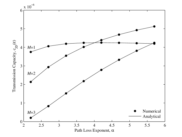
Figure 13: Transmission capacity vs. path loss exponent of slotted ALOHA with spatial multiplexing using ZF receivers in the interference-limited regime, and with ${r_{\rm tr}}=3$ m, $\beta=3$ dB, $\epsilon=0.0001$ and $p=1$.

Proposition 2 also provides a useful design criteria for choosing how many data streams should be transmitted for a given path loss exponent. For example, for ZF, when $\alpha=4$ and at high transmit SNR $\rho$, we see in (82) that the optimal number of transmitted data streams should be half the number of receive antennas. The optimal number of transmit antennas was also considered in [8], which considered the use of MMSE receivers to cancel the interference from the closest transmitting nodes and a single-link performance measure. In contrast, we consider the use of ZF receivers to cancel interference from the corresponding transmitter only, and a network performance measure.

V-A1 Comparison with Multi-Node Interference Cancelation (Single-Input Multiple-Output with Partial Zero-Forcing)

Linear scaling was also previously shown to occur in [10] for single-stream transmission, i.e., $M=1$, by employing a partial zero forcing (PZF) scheme, where the receive antennas were used to simultaneously cancel the interference from the $k_{\rm PZF}$ closest interfering nodes and boost the signal power from the corresponding transmitter. Specifically, the transmission capacity of the PZF scheme at high transmit SNR $\rho$ was shown to scale as

$${\rm c}_{\rm PZF}(\epsilon)=\Theta\left(k_{\rm PZF}\left(\frac{N-k_{\rm PZF}}{k_{\rm PZF}}\right)^{\frac{2}{\alpha}}\right)\;.$$ (86)

Linear scaling was then achieved by setting $k_{\rm PZF}=\kappa N$ where $0<\kappa<1$. At high transmit SNR $\rho$, comparing (80) and (86), we see that setting $k_{\rm PZF}=M$ results in the PZF scheme achieving the same scaling as our spatial multiplexing with ZF receivers scheme.

To understand the reason behind this same linear scaling result, we explore some similarities between our spatial multiplexing with ZF receivers scheme and the PZF scheme in [10]. For both schemes, it can be shown that the signal component contributes to the transmission capacity scaling by a factor of $N^{\frac{2}{\alpha}}$, and is achieved by allocating $N(1-\kappa)$ d.o.f. to boost the signal power, where $0<\kappa<1$. The key difference, however, lies with how the remaining $N\kappa$ d.o.f. are used. For our spatial multiplexing with ZF receivers scheme, the $N\kappa$ d.o.f. are used to cancel interference from the corresponding transmitting node, while for the PZF scheme, they are used to cancel interference from the $k_{\rm PZF}=N\kappa$ closest interferers. However, it turns out that the resulting interference component of both schemes contributes to the transmission capacity through the same scaling factor, which is $N^{1-\frac{2}{\alpha}}$. To see why, it is convenient to express the transmission capacity (34) in the alternative form

$${\rm c}_{\rm ZF}(\epsilon)=\lambda^{*}(\epsilon)(1-\epsilon)$$ (87)

where $\lambda^{*}(\epsilon)$ is the inverse of $\epsilon={\rm F}_{\rm ZF}\left(\beta;\frac{\lambda}{M}\right)$ taken w.r.t. $\lambda$. This alternate form can be obtained by noting that

$$\epsilon={\rm F}(\beta;\lambda/M)\quad\Rightarrow\quad\lambda=M{\rm F}^{-1}(\epsilon),$$ (88)

which has the same form as (34) for small $\epsilon$. (87) indicates that from a transmission capacity perspective, increasing the number of data streams $M$ has the same effect as decreasing the density of transmitting nodes by a factor of $M$.

From the modified transmission capacity definition (87), we can now explain why for both schemes the interference component contributes to the transmission capacity by the same scaling factor. First, for spatial multiplexing with ZF receivers, the average distance from the receiver to the closest interfering node, where the interfering nodes are distributed with density $\lambda/M$, can be shown to scale as $\sqrt{M}$ [27, Eq. (9)] whereas for PZF (after cancelation), it scales as $\sqrt{k_{\rm PZF}}$ [10]. Thus, with $M=k_{\rm PZF}$, these coincide. Second, for both schemes, the average number of interfering data streams per unit area is the same, given by $\lambda$. For spatial multiplexing with ZF, this can be seen by noting that $M$ data streams are being transmitted by $\lambda/M$ nodes per unit area.

Summing up, the key point of the discussion above is that the same linear transmission capacity scaling can be achieved whether we employ MIMO with ZF receivers, or SIMO with PZF. Clearly, the choice as to which scheme to employ in practice will depend on the specific network design. When there is the capability for employing multiple antennas on all nodes, MIMO with ZF will be more attractive, since it has lower complexity and less stringent requirements on the level of channel knowledge at the receivers. On the other hand, if single-antenna transmitters are required (e.g., due to size limitations, relevant for sensor networks), then SIMO with PZF will be appropriate. A key implementation issue for such networks, however, is how to accurately estimate the multi-node interference which is needed to perform interference cancelation at each receiver. Whilst very well motivated in theory, some important questions still remain as to the practical feasibility of this approach.

V-B Transmission Capacity of OSTBC

We now consider the transmission capacity of OSTBC at low outage probabilities $\epsilon$. In this case, analogous to (80), we consider the case where $N$ grows large, and also assume that $\beta$ and $\epsilon$ are selected such that $\epsilon>{\rm F}^{\rm SU}(\beta)$. Moreover, we consider high transmit SNRs $\rho$, and thus, substituting the relevant parameters from Table I into (66), we get

$$\tilde{{\rm c}}_{\rm OSTBC}(\epsilon) =\Theta\left(g(M)N^{\frac{2}{\alpha}}\right)$$ (89)

where

$$g(M)=R(M)M^{\frac{2}{\alpha}}\frac{\Gamma\left(\frac{N_{I}(M)}{M}\right)}{\Gamma\left(\frac{N_{I}(M)}{M}+\frac{2}{\alpha}\right)}$$ (90)

where we have made explicit the dependence of the code rate $R$ and $N_{I}$ on $M$. (Note that this result applies for arbitrary values of $M$.) In general, there is no simple relationship characterizing the dependence of $R$ and $N_{I}$ on $M$. Thus, to proceed, here we consider the extreme scenarios pertaining to minimum-rate and maximum-rate codes.

For minimum-rate codes, i.e., cyclic diversity systems, $R(M)=1/M$ and $N_{I}(M)=M$. Thus, it follows that $\tilde{{\rm c}}_{\rm OSTBC}(\epsilon)=\Theta\left(M^{\frac{2}{\alpha}-1}N^{\frac{2}{\alpha}}\right)$, which is obviously maximized if $M=1$, yielding $\tilde{{\rm c}}_{\rm OSTBC}(\epsilon)=\Theta\left(N^{\frac{2}{\alpha}}\right)$. This special case simply corresponds to a standard SIMO system.

For maximum-rate codes, e.g., the Alamouti code, it is known from [22] that for $M$ even

$$\frac{1}{2}<R(M)\leq\frac{M+2}{2M},\qquad N_{I}(M)=\frac{M(M+2)}{2}$$ (91)

and for $M$ odd

$$\frac{1}{2}<R(M)\leq\frac{M+3}{2(M+1)},\qquad\frac{M(M+1)}{2}\leq N_{I}(M)<\frac{M(M+2)}{2}\;.$$ (92)

Thus, using these bounds and the inequality $\frac{m^{x}}{\Gamma(1-x)}\leq\frac{\Gamma(m)}{\Gamma(m-x)}\leq m^{x}$ [12], we have $g^{\rm lb}(M)\leq g(M)\leq g^{\rm ub}(M)$, where

$$g^{\rm lb}(M):=\frac{1}{2\Gamma\left(1+\frac{2}{\alpha}\right)}\left(\frac{2M}{M+2}\right)^{\frac{2}{\alpha}}$$

$$g^{\rm ub}(M):=\begin{cases}&\left(\frac{2M}{M+2}\right)^{\frac{2}{\alpha}-1},\hskip 51.21504pt{\rm even}\;M\\ &\frac{M+3}{2(M+1)}\left(\frac{2M}{M+1}\right)^{\frac{2}{\alpha}},\hskip 28.45274pt{\rm odd}\;M\\ \end{cases}\;.$$ (93)

From this, it is clear that, regardless of whether $M$ is kept fixed or allowed to vary with $N$, the best achievable scaling is $\tilde{{\rm c}}_{\rm OSTBC}(\epsilon)=\Theta\left(N^{\frac{2}{\alpha}}\right)$. This result, combined with that for minimum-rate codes above, indicates that OSTBC can only achieve sub-linear scaling, in contrast to the spatial multiplexing systems considered previously.

We now consider the question of how to select $M$ to maximize the transmission capacity scaling for large $N$. This is tantamount to maximizing the leading multiplicative factor $g(M)$. For maximum-rate codes, we will focus on $g^{\rm up}(M)$, since it serves as an accurate approximation for $g(M)$. It is obvious that $g^{\rm up}(M)$ is maximized by selecting $M=2$ for $M\geq 2$. Thus, the key finding is that for OSTBC, either the Alamouti code or SIMO transmission should be employed. Although it is hard to obtain a simple design rule which specifies which of these two coding schemes will perform better under certain network conditions, we can gain insights by numerical analysis. In particular, Fig. 14 plots the transmission capacity achieved by OSTBC for different $M$. Results are presented for $N=3$, and the codes used for $M=2$ and $M=3$ are the maximum-rate codes given by (24) and (45) respectively. The “Analytical” curves are based on (66), and are clearly seen to match with the “Numerical” curves, obtained by taking $\rho$ large in the outage probability expression obtained by substituting the relevant parameters from Table I into (1), and subsequently solving for $\lambda(\epsilon)$ using numerical techniques. We see that the Alamouti code performs better than SIMO for $\alpha<4.7$, and vice-versa for $\alpha>4.7$.

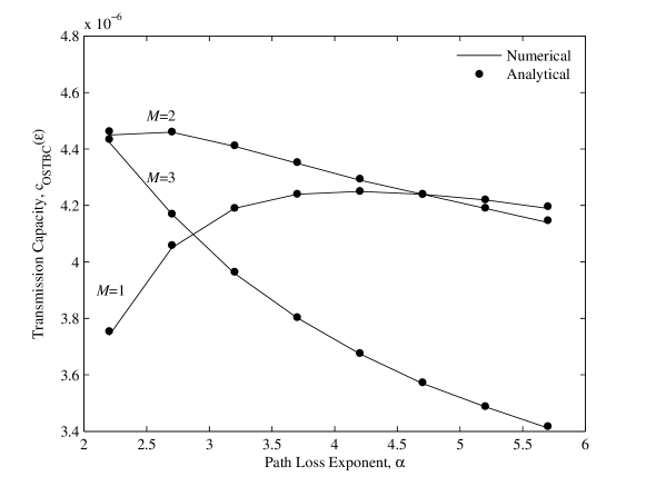
Figure 14: Transmission capacity vs. path loss exponent of slotted ALOHA with OSTBC, and with ${r_{\rm tr}}=3$ m, $\beta=3$ dB, $\epsilon=0.0001$ and $p=1$.

V-C Comparison

For large $N$ and assuming $\epsilon>{\rm F}^{\rm SU}(\beta)$ in (66), spatial multiplexing achieves a higher transmission capacity scaling than OSTBC, at high transmit SNR $\rho$, if

$$\begin{array}[]{ll}&R(M)<\frac{M}{\Gamma\left(1+\frac{2}{\alpha}\right)}\left(\frac{N_{I}(M)}{M^{3}}\left(1-\frac{M}{N}\right)\right)^{\frac{2}{\alpha}}\quad\quad{\rm for\;ZF}\\ &R(M)<\frac{M}{\Gamma\left(1+\frac{2}{\alpha}\right)}\left(\frac{N_{I}(M)}{M^{3}}\left(1-\frac{M\beta}{N}\right)\right)^{\frac{2}{\alpha}}\hskip 11.38092pt{\rm for\;MRC}\;.\end{array}$$ (96)

Clearly, these conditions depend on the specific OSTBC employed. As expected, we see that by incorporating a higher rate code, whilst keeping all other parameters fixed, the possibility of the condition (96) being satisfied is decreased. Moreover, by noting that $N_{I}(M)<M^{3}$ for all practical OSTBC codes, the condition in (96) becomes more likely to be satisfied as the path loss exponent $\alpha$ increases; indicating that environments with higher path loss exponents are more beneficial for spatial multiplexing, compared with OSTBC; and vice-versa for low path loss environments.

Figs.  15 and 16 show the transmission capacity achieved by spatial multiplexing with ZF receivers and OSTBC for different antenna configurations. The curves for both spatial multiplexing and OSTBC are based on (66). The results show that the relative transmission capacity of the transmission schemes depends on both the antenna configuration, the path loss exponent $\alpha$ and the SINR operating value. In particular, we observe that OSTBC performs best at small $\alpha$ (e.g., $\alpha=2$, corresponding to free space environments), whereas spatial multiplexing performs the best at large $\alpha$ (e.g., $\alpha=6$, corresponding to indoor environments). These observations agree with our analytical conclusions put forth above, based on (96).

We also observe that ZF receivers are preferable over MRC receivers for a sufficiently high SINR operating value, i.e., $\beta=0$ dB, and vice-versa for a low SINR operating value, i.e., $\beta=-5$ dB. This is because for high SINR operating values, the outage probability when there is no multi-node interference, i.e., the outage probability of the single user MIMO system, is higher for MRC than ZF, and offsets any positive gains resulting from the signal power that MRC has over ZF receivers. However, for sufficiently low SINR operating values, and as indicated by previous analysis, the outage probability when there is no multi-node interference is negligible for both receivers, and thus MRC is preferable over ZF.

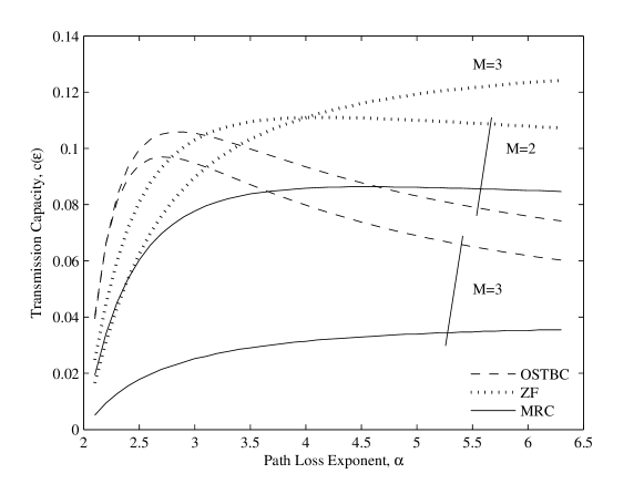
Figure 15: Transmission capacity vs. path loss exponent of slotted ALOHA with spatial multiplexing and OSTBC, and with $N=5$, ${r_{\rm tr}}=1$ m, $\beta=0$ dB, $N=5$, $\rho=30$ dB, $\epsilon=0.15$ and $p=1$.

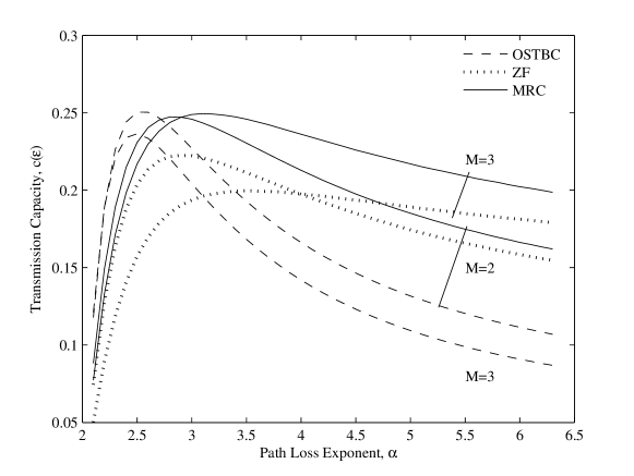
Figure 16: Transmission capacity vs. path loss exponent of slotted ALOHA with spatial multiplexing and OSTBC, and with $N=5$, ${r_{\rm tr}}=1$ m, $\beta=-5$ dB, $N=5$, $\rho=30$ dB, $\epsilon=0.15$ and $p=1$.

VI Network Throughput Comparison between Slotted ALOHA and Coordinated Access protocol

In this section, we compare the multi-antenna transmission schemes employing a slotted ALOHA MAC protocol, described in Section II, with a baseline single antenna transmission scheme employing a CA MAC protocol. It is worth noting that the CA protocol is an idealized protocol, since the overhead involved in achieving full coordination is prohibitive in practice for ad hoc networks. We will show that the simple multi-antenna slotted ALOHA MAC protocol can in fact yield even higher throughputs than the tightly scheduled CA MAC protocol in various practical scenarios. This shows that not only does the use of multiple antennas allow for a decentralized MAC, but it can actually also improve throughput in certain scenarios. We start by describing the CA protocol model.

VI-A Coordinated Access Protocol Model

For the CA protocol, transmissions are scheduled such that interference is minimized at each receiver. Since the strongest interferers are those closest to the receivers, we consider a CA scheduling protocol which removes the closest interferers within a guard zone around each receiver. Note that, although removing these strong interferers leads to a gain in throughput, this gain comes at the cost of significant overhead and synchronization requirements; something which is clearly undesirable in an ad hoc network setting.

Scheduling nodes to minimize interference has been considered for a long time, however there have been few results where the transmitting nodes form a PPP. In [28], a circular guard zone of radius $r_{\rm gz}$ around the typical receiver was considered, but neglected a guard zone around every other receiver in the network. Recently in [7], transmissions were scheduled only if the receiver has no interferers within a circular guard zone also of radius $r_{\rm gz}$. However, the throughput suffers when the network becomes dense, as the probability of a receiver with no interferers within its guard zone decreases.

In this section, we consider an alternative model where transmissions are scheduled in a TDMA manner. As with other common CA protocols, the throughput of the TDMA scheme we consider does not go to zero as the network becomes dense. For analytical tractability, we assume each receiver is located at the center of a non-overlapping square of side length $2r_{\rm gz}$, arranged according to a lattice structure. The transmitting nodes, distributed according to a PPP, which lie in the same square are each assigned a time slot of the same duration as the slots used in the slotted ALOHA protocol. We assume a dynamic slot allocation where the number of slots in a particular square is equal to the number of transmitters in that square. We note that although this may not be completely practical due to the deterministic placement of each receiver, this model correctly captures the fact that each receiver is spatially separated such that interference is minimized, and is very useful for comparison purposes.

The CA protocol is illustrated in Fig. 17, where we show a network before and after scheduling. The scheduled transmitter transmits to the receiver at the center of the corresponding square during the assigned time slot. In Fig. 17, the receivers are shown as crosses, while transmitters as dots. As shown, after applying the CA protocol, there is at most one transmitter in each square, which transmits to the receiver at the center of the square.

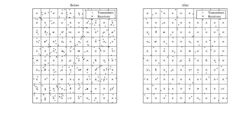
Figure 17: Coordinated access protocol model: before and after scheduling with $\lambda=3$ ${\rm m}^{2}$.

Under this model, the following theorem presents a new closed-form upper bound for the network throughput.

Theorem 3

The throughput of the CA MAC protocol employing single antennas is upper bounded by

$${\rm T}_{\rm CA}\leq e^{-\frac{\beta r_{\rm tr}^{\alpha}}{\rho}}\lambda_{\rm CA}\exp\left\{-\pi\lambda_{\rm CA}\left(\frac{2(\beta r_{\rm tr}^{\alpha})^{\frac{2}{\alpha}}\Gamma\left(\frac{2}{\alpha}\right)\Gamma\left(1-\frac{2}{\alpha}\right)}{\alpha}-\left(\frac{2r_{\rm gz}}{\sqrt{\pi}}\right)^{2}\;_{2}F_{1}\left(\frac{2}{\alpha},1;1+\frac{2}{\alpha};-\left(\frac{2r_{\rm gz}}{\sqrt{\pi}r_{\rm tr}}\right)^{\alpha}\frac{1}{\beta}\right)\right)\right\}$$ (97)

where $\lambda_{\rm CA}=(1-e^{-4\lambda r_{\rm gz}^{2}})/(4r_{\rm gz}^{2})$, and ${}_{2}F_{1}(\cdot,\cdot;\cdot;\cdot)$ is the Gauss hypergeometric function [24, Eq. (9.6.2)].

Proof:

See the Appendix -E. ∎

Note that the same throughput can also be obtained by considering an alternative but similar system where the transmitting nodes around the square guard zone transmit with probability $(1-e^{-4\lambda r_{\rm gz}^{2}})/(4\lambda r_{\rm gz}^{2})$ at each time slot. Thus the transmission probability of the CA protocol adaptively adjusts to the intensity of transmitting nodes. This is in contrast to the fixed transmission probability employed in slotted ALOHA.

For the case of dense networks, the throughput of the CA protocol approaches a constant as $\lambda\to\infty$, and is given by substituting $\lambda_{\rm CA}=\lambda_{\rm CA}^{\infty}=1/4r_{\rm gz}^{2}$ into (97). This constant value reflects the fact that the CA protocol ensures that only one node within a square of length $2r_{\rm gz}$ is allowed to transmit. This models, for example, a system using a TDMA protocol when a large number of transmitting nodes causes the throughput to reach a saturation point, and the only transmitting nodes are the ones allocated to the time slot corresponding to the current transmission period.

Fig. 18 presents the throughput vs. the guard zone parameter $r_{\rm gz}$ for different intensities. We see that the analytical upper bounds in (97) accurately match the Monte Carlo simulated curves in most cases. We also notice that there is an optimal value of $r_{\rm gz}$ which maximizes the throughput of the system. In addition, we see that the dense network throughput, obtained by substituting $\lambda_{\rm CA}^{\infty}$ into (97), closely matches the Monte Carlo simulated curves for transmitting node intensities as small as 0.03.

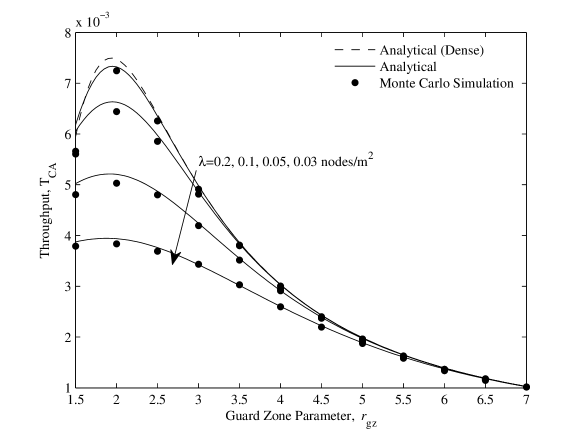
Figure 18: Throughput of the CA protocol vs. guard zone parameter with $\rho=10$ dB, $r_{\rm tr}=1.5$ m, $\alpha=4$ and $\beta=5$ dB.

VI-B Comparison

In this section, we compare the slotted ALOHA MAC protocol employing multiple antennas with the CA MAC protocol employing single antennas. When considering the CA protocol we choose the guard zone parameter $r_{\rm gz}$ which maximizes the throughput for each value of $\lambda$. Also, when considering the slotted ALOHA protocol we only utilize one transmit antenna and multiple receive antennas. Note that our analysis in Sections III and IV shows that utilizing more transmit antennas for spatial multiplexing and OSTBC may lead to a higher throughput in different networking scenarios. However, as our purpose is to show the practicality of the slotted ALOHA protocol, we consider the simple case when only one transmit antenna is utilized. Note that in this scenario, the performance of spatial multiplexing and OSTBC are the same. We assume both protocols use the same initial intensity of transmitting nodes $\lambda$, thereby allowing for a fair comparison.

Fig. 19 presents the intensities and transmission probabilities for which the throughput of slotted ALOHA is greater than for the CA protocol. Results are presented for different antenna configurations, and the respective throughput values are calculated from (33) and (97). Note that the throughput for slotted ALOHA can also be obtained from (33). We clearly see that increasing the number of receive antennas leads to an increase in the intensity range for which the slotted ALOHA throughput is greater than the CA throughput.

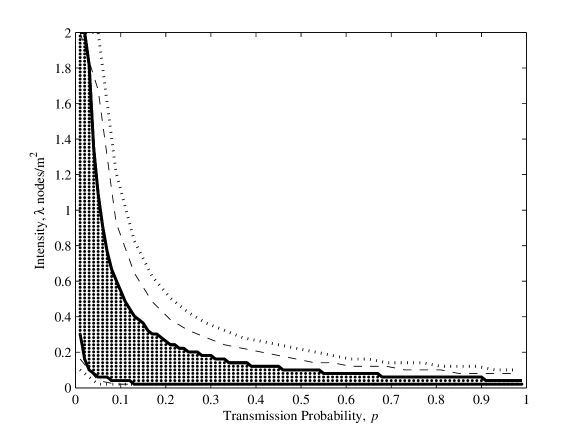
Figure 19: Comparison between slotted ALOHA and the CA protocol. The shaded area between the solid lines shows the region where the throughput of slotted ALOHA with $M=1$ in (33) is greater than the CA protocol in (97); for $N=2$. The dashed lines shows that the region expands for $N=3$, and the dotted lines shows further expansion for $N=4$. Results are shown for $M=1$, $\rho=10$ dB, $r_{\rm tr}=2$ m, $\alpha=3$ and $\beta=5$ dB.

In addition, Fig. 19 shows that slotted ALOHA outperforms the CA protocol for nearly all transmission probability values when the network is sparse. However, as the intensity increases, the transmission probability has to decrease in order for the throughput of slotted ALOHA to be greater than the CA protocol. Although not shown in Fig. 19, the throughput is an increasing function of the number of antennas.

VII Conclusion

Open-loop point-to-point transmission schemes and slotted ALOHA MAC are practical choices for ad hoc networks, due to their relatively low feedback requirements and decentralized structure, respectively. Within this framework we have analyzed important network performance measures for spatial multiplexing transmission with MRC and ZF receivers, and for OSTBC, using tools from stochastic geometry. We derived new expressions for the outage probability, which were subsequently used to evaluate the network throughput and transmission capacity.

Based on our analysis, we demonstrated that the optimal number of transmit antennas, and the relative performance of the spatial multiplexing and OSTBC systems is dependent on a number of system parameters, including the chosen SINR operating value and node intensity. In particular, from a throughput perspective, our analysis has led to the following design guidelines:

• For dense networks and high SINR operating values, cyclic antenna diversity codes utilizing the maximum number of transmit antennas is the preferred scheme.

• For low SINR operating values, spatial multiplexing with MRC receivers, while transmitting with the maximum number of data streams, is the preferred scheme.

For applications operating under a strict outage constraint, the transmission capacity is a preferable performance measure. From a transmission capacity perspective, the following were observed:

• For sufficiently high path loss exponents, spatial multiplexing is preferred over OSTBC, and vice-versa for low path loss exponents.

• In the large antenna $N$ regime, and if the self-interference is sufficiently smaller than the SINR operating value:

  • MRC and ZF receivers can achieve linear scaling, while OSTBC can only achieve sub-linear scaling.

  • For OSTBC, either the Alamouti scheme or SIMO is the optimal scheme, depending on the path loss exponent and number of receive antennas.

Finally, we demonstrated the practicality of the multi-antenna slotted ALOHA MAC system in ad hoc networks, by comparing it with a baseline single antenna CA MAC system. We showed the interesting result that in many practical scenarios, the multi-antenna slotted ALOHA MAC system can actually outperform the idealized single antenna CA MAC in terms of network throughput. Further, we demonstrated that increasing the number of antennas can have the benefit of increasing the range of node intensities for which the use of slotted ALOHA MAC outperforms the idealized single antenna CA MAC.

VIII Acknowledgments

The authors would like to thank Prof. Nihar Jindal for useful discussions regarding the linear scaling of spatial multiplexing.

-A Derivation of SINR Approximation for OSTBC

We require the following lemmas:

Lemma 1

Let $\mathbf{h}\stackrel{{\scriptstyle d}}{{\sim}}\mathcal{CN}_{N\times 1}\left(\mathbf{0}_{N\times 1},\mathbf{I}_{N}\right)$ and $\mathbf{g}\stackrel{{\scriptstyle d}}{{\sim}}\mathcal{CN}_{N\times 1}\left(\mathbf{0}_{N\times 1},\mathbf{I}_{N}\right)$ be independent random variables. Then

$$\frac{|\mathbf{h}^{\dagger}\mathbf{g}|^{2}}{||\mathbf{h}||^{2}}\stackrel{{\scriptstyle d}}{{\sim}}{\rm Gamma}(0,1)$$ (98)

is independent of $\mathbf{h}$.

Proof:

See [29]. ∎

Lemma 2

Let $\mathbf{h}\stackrel{{\scriptstyle d}}{{\sim}}\mathcal{CN}_{N\times 1}\left(\mathbf{0}_{N\times 1},\mathbf{I}_{N}\right)$,
$\mathbf{g}\stackrel{{\scriptstyle d}}{{\sim}}\mathcal{CN}_{N\times 1}\left(\mathbf{0}_{N\times 1},\mathbf{I}_{N}\right)$, $x\stackrel{{\scriptstyle d}}{{\sim}}\mathcal{CN}(0,1)$ and $y\stackrel{{\scriptstyle d}}{{\sim}}\mathcal{CN}(0,1)$, all mutually independent. Then

$$|\mathbf{h}^{\dagger}\mathbf{g}|^{2}<_{\rm st}|\mathbf{h}^{\dagger}\mathbf{g}+xy|^{2}$$ (99)

where

$$A<_{\rm st}B\;\;\Longrightarrow\;\;{\rm F}_{A}(z)>{\rm F}_{B}(z),\quad{\rm for}\;z\in\mathds{R}^{+},$$ (100)

for random variables $A$ and $B$ with c.d.f.s ${\rm F}_{A}(\cdot)$ and ${\rm F}_{B}(\cdot)$ respectively.

Proof:

Setting $X_{1}=\mathbf{h}^{\dagger}\mathbf{g}$, the distribution of $X_{1}$ conditioned on $\mathbf{h}$ is $\mathcal{CN}\left(0,||\mathbf{h}||_{F}^{2}\right)$. Thus, $|X_{1}|^{2}$ conditioned on $\mathbf{h}$ has the same distribution as $||\mathbf{h}||_{F}^{2}Y_{1}$, where $Y_{1}\stackrel{{\scriptstyle d}}{{\sim}}{\rm Exp}(1)$. Similarly, setting $X_{2}=\mathbf{h}^{\dagger}\mathbf{g}+xy$, $|X_{2}|^{2}$ conditioned on $\mathbf{h}$ has the same distribution as $\left(||\mathbf{h}||_{F}^{2}+|x|^{2}\right)Y_{2}$, where $Y_{2}\stackrel{{\scriptstyle d}}{{\sim}}{\rm Exp}(1)$. (99) now follows. ∎

Lemma 3

Let $X_{i}\stackrel{{\scriptstyle d}}{{\sim}}{\rm Gamma}\left(k_{\ell},\theta\right)$, for $i=1,\ldots,L$, all mutually independent. Then

$$\sum_{i=1}^{L}X_{i}\stackrel{{\scriptstyle d}}{{\sim}}{\rm Gamma}\left(\sum_{i=1}^{L}k_{i},\theta\right)\;.$$ (101)

Proof:

See [30]. ∎

Lemma 4

Let $X_{1}\stackrel{{\scriptstyle d}}{{\sim}}{\rm Gamma}(k_{1},\theta)$ and $X_{2}\stackrel{{\scriptstyle d}}{{\sim}}{\rm Gamma}(k_{2},\theta)$. If $k_{1}>k_{2}$, then

$${\rm E}\left[X_{1}^{n}\right]>{\rm E}\left[X_{2}^{n}\right]$$ (102)

for any $n\in\mathds{Z}^{+}$.

Proof:

The $n$th moment of $X\stackrel{{\scriptstyle d}}{{\sim}}{\rm Gamma}\left(k,\theta\right)$ is

$${\rm E}\left[X^{n}\right] =\frac{\Gamma(n+k)\theta^{n}}{\Gamma(k)}\;.$$ (103)

The proof follows upon showing the positivity of the derivative of (103) w.r.t. $k$. ∎

Lemma 5

Let $\mathbf{h}\stackrel{{\scriptstyle d}}{{\sim}}\mathcal{CN}_{L\times 1}\left(\mathbf{0}_{L\times 1},\mathbf{I}_{L}\right)$, $\mathbf{g}\stackrel{{\scriptstyle d}}{{\sim}}\mathcal{CN}_{L\times 1}\left(\mathbf{0}_{L\times 1},\mathbf{I}_{L}\right)$ and $\mathbf{y}\stackrel{{\scriptstyle d}}{{\sim}}\mathcal{CN}_{T\times 1}\left(\mathbf{0}_{T\times 1},\mathbf{I}_{T}\right)$, all mutually independent. Then $Z=\frac{|\mathbf{h}^{\dagger}\mathbf{g}|^{2}}{||\mathbf{h}||^{2}+||\mathbf{y}||^{2}}$ has approximately the same distribution as

$$Z^{\approx}\stackrel{{\scriptstyle d}}{{\sim}}{\rm Gamma}\left(\frac{L}{L+T},1\right).$$ (104)

Proof:

We justify this approximation by first noting that ${\rm E}[Z]={\rm E}[Z^{\approx}]$. Also, applying Lemma 1 and Lemma 4 to $Z$ yields: $Z^{\rm lb}<Z\leq Z^{\rm ub}$, where $Z^{\rm lb}\stackrel{{\scriptstyle d}}{{\sim}}\lim_{\varsigma\to 0}{\rm Gamma}\left(\varsigma,1\right)$ and $Z^{\rm ub}\stackrel{{\scriptstyle d}}{{\sim}}{\rm Gamma}\left(1,1\right)$. Now, $Z\to Z^{\rm lb}$ when $L\to 0$ and $Z\to Z^{\rm ub}$ when $L\to L+T\Rightarrow T\to 0$, implying that $Z\to Z^{\approx}$ at the two extremes: $\frac{L}{L+T}\to 0$ and $\frac{L}{L+T}\to 1$. For values away from these two extremes, our approximation is motivated by noting that for a fixed $L+T$, applying Lemma 2 to $Z$ and Lemma 4 to $Z^{\approx}$ reveals, respectively, that $Z$ and $Z^{\approx}$ both increase with $L$. ∎

We are now in a position to derive our approximation for the OSTBC SINR. We first outline the main issues which make dealing with the exact SINR (28) difficult, and provide some justification for our approximations which are used to overcome these.

• The first challenge is caused by mutual dependencies between random variables in the SINR. In particular, the normalized interference power, $\mathcal{K}_{\ell,\sum}$, is comprised of a sum of dependent random variables. As in [12, 23], we will neglect this mutual dependence, which is justified in [23] by noticing that the common terms in $\mathcal{K}_{\ell,\sum}$ are multiplied by independent random variables, so they should be “nearly independent”. In addition, the numerator and denominator in (28) are dependent. Once again, as in [23], we neglect this dependence, with the argument that there are sufficient independent terms in the numerator and denominator that the dependence is weak.

• The second challenge is the difficulty in computing the exact marginal distribution of $\mathcal{K}_{\ell,\sum}$ analytically, even under the independence assumption discussed above. This appears intractable, and to address this we seek an accurate approximation by fitting a gamma distribution. Such distributions are known to be exact for various cases and are expected to be quite accurate in general. They are also analytically friendly, allowing us to invoke the useful properties given in the lemmas above.

To most clearly illustrate our methods, we will first present our derivations for a specific OSTBC code; namely, the OSTBC code in (44). We will then give a brief discussion to highlight how the derivation extends to general OSTBC codes. It is convenient to define the operator ${\rm vecdim}(\cdot)$, which takes as input the inner product of two vectors with equal dimension, and returns the dimension of these vectors.

-A1 Derivation for the OSTBC Code in (44)

Without loss of generality, we focus on decoding $x_{0,1}$. The $\ell$th row of $\varsigma_{k}(\mathbf{V})$ and $\mathbf{M}_{k}$ are given respectively by

$$\varsigma_{k}(\mathbf{V})_{\ell}=\left[\mathbf{V}_{\ell,1},\hskip 5.69046pt\mathbf{V}_{\ell,2}^{*},\hskip 5.69046pt-\mathbf{V}_{\ell,3}^{*},\hskip 5.69046pt-\mathbf{V}_{\ell,4}\right]\hskip 5.69046pt{\rm and}$$

$$\left(\mathbf{M}_{k}\right)_{\ell}=\left[h_{0,\ell,1}^{*},\hskip 5.69046pth_{0,\ell,2},\hskip 5.69046pth_{0,\ell,3},\hskip 5.69046pth_{0,\ell,4}^{*}\right]\;.$$ (105)

Substituting (44) and (-A1) into (27), the data estimate for $x_{0,1}$ can be written as

$$\hat{x}_{0,1}=||\mathbf{H}_{0}||_{F}^{2}x_{0,1}+\sum_{D_{\ell}\in\Phi}\sqrt{\frac{1}{|D_{\ell}|^{\alpha}}}I_{\ell}+\sum_{k=1}^{N}\left(h_{0,k,1}^{*}n_{k,1}+h_{0,k,2}n_{k,2}^{*}-h_{0,k,3}n_{k,3}^{*}-h_{0,k,4}^{*}n_{k,4}\right)$$

where

$$I_{\ell} =W_{\ell,1}x_{\ell,1}+W_{\ell,2}x_{\ell,2}+Z_{\ell,2}x_{\ell,2}^{*}+W_{\ell,3}x_{\ell,3}+Z_{\ell,3}x_{\ell,3}^{*}\;,$$ (107)

with

$$W_{\ell,1} =\sum_{k=1}^{N}\left(h_{0,k,1}^{*}h_{\ell,k,1}+h_{0,k,2}h_{\ell,k,2}^{*}+h_{0,k,3}h_{\ell,k,3}^{*}+h_{0,k,4}^{*}h_{\ell,k,4}\right)\;,$$ (108)

$$W_{\ell,2}=\sum_{k=1}^{N}\left(h_{0,k,1}^{*}h_{\ell,k,2}-h_{0,k,2}h_{\ell,k,1}^{*}\right)$$

$$Z_{\ell,2}=\sum_{k=1}^{N}\left(-h_{0,k,3}h_{\ell,k,4}^{*}+h_{0,k,4}^{*}h_{\ell,k,3}\right)\;,$$ (109)

$$W_{\ell,3}=\sum_{k=1}^{N}\left(h_{0,k,1}^{*}h_{\ell,k,3}-h_{0,k,3}h_{\ell,k,1}^{*}\right)$$

$$Z_{\ell,3}=\sum_{k=1}^{N}\left(h_{0,k,2}h_{\ell,k,4}^{*}-h_{0,k,4}^{*}h_{\ell,k,2}\right)\;.$$ (110)

Note that the $W_{\ell,q}$’s and $Z_{\ell,q}$’s can each be interpreted as the inner product of two equal-length vectors; in each case, with one vector having elements drawn from either $\pm\mathbf{H}_{0}$ or $\pm\mathbf{H}_{0}^{\dagger}$, and the other vector having elements drawn from either $\pm\mathbf{H}_{\ell}$ or $\pm\mathbf{H}_{\ell}^{\dagger}$. For example, $W_{\ell,2}$ in (-A1) can be written as

$$W_{\ell,2}=\mathbf{w}_{0}\cdot\mathbf{w}_{\ell}$$ (111)

where $\mathbf{w}_{0}$ and $\mathbf{w}_{\ell}$ are $2N\times 1$ vectors given respectively by

$$\mathbf{w}_{0}=[h_{0,1,1}^{*},\,-h_{0,1,2},\,\ldots\,,h_{0,N,1}^{*},\,-h_{0,N,2}]^{T}$$ (112)

and

$$\mathbf{w}_{\ell}=[h_{\ell,1,2},\,h_{\ell,1,1}^{*},\,\ldots,\,h_{\ell,N,2},\,h_{\ell,N,1}^{*}]^{T}\;.$$ (113)

With this interpretation, it is clear that ${\rm vecdim}(W_{\ell,1})=4N$ and ${\rm vecdim}(W_{\ell,2})={\rm vecdim}(Z_{\ell,2})={\rm vecdim}(W_{\ell,3})={\rm vecdim}(Z_{\ell,3})=2N$.

From (-A1), the SINR can be written as

$$\gamma_{{\rm OSTBC},1} =\frac{\frac{\rho}{RMr_{\rm tr}^{\alpha}}||\mathbf{H}_{0}||_{F}^{2}}{\frac{\rho}{RM}\sum_{D_{\ell}\in\Phi}\frac{1}{|D_{\ell}|^{\alpha}}\mathcal{K}_{\ell,\sum}+1}\;$$ (114)

where $\mathcal{K}_{\ell,\sum}=\frac{{\rm E}_{x_{\ell,1},x_{\ell,2},x_{\ell,3}}\left[I_{\ell}I_{\ell}^{*}\right]}{||\mathbf{H}_{0}||_{F}^{2}}$. Note that

$$\mathcal{K}_{\ell,\sum} =\mathcal{K}_{\ell,1}+\mathcal{K}_{\ell,2}+\mathcal{K}_{\ell,3}$$ (115)

where

$$\mathcal{K}_{\ell,1}=\frac{|W_{\ell,1}|^{2}}{||\mathbf{H}_{0}||_{F}^{2}}$$ (116)

and, for $q=2,3$,

$$\mathcal{K}_{\ell,q} =\frac{{\rm E}_{x_{\ell,q}}\left[\bigl{|}W_{\ell,q}x_{\ell,q}+Z_{\ell,q}x_{\ell,q}^{*}\bigr{|}^{2}\right]}{||\mathbf{H}_{0}||_{F}^{2}}$$

$$=\frac{|W_{\ell,q}|^{2}+|Z_{\ell,q}|^{2}}{||\mathbf{H}_{0}||_{F}^{2}}.$$ (117)

It is clear that all three terms in (115) are mutually dependent. Moreover, there is dependence within each term, since $|W_{\ell,q}|^{2}$, $|Z_{\ell,q}|^{2}$, and $||\mathbf{H}_{0}||_{F}^{2}$ involve common elements. As stated previously, we neglect these dependencies. Thus applying Lemma 5 to $\frac{|W_{\ell,q}|^{2}}{||\mathbf{H}_{0}||_{F}^{2}}$ and $\frac{|Z_{\ell,q}|^{2}}{||\mathbf{H}_{0}||_{F}^{2}}$, followed by applying Lemma 3 reveals that $\mathcal{K}_{\ell,q}$ is approximately distributed as

$${\rm Gamma}\left({\rm vecdim}(W_{\ell,q})+{\rm vecdim}(Z_{\ell,q}),1\right)$$ (118)

for all $q=1,2,3$. (Note that for the particular code considered here, $Z_{\ell,1}=0$.) Now, from (44) and (107), it can be seen that

$$\sum_{q=1}^{N_{s}}{\rm vecdim}(W_{\ell,q})+{\rm vecdim}(Z_{\ell,q})=NN_{I}\,,$$ (119)

and we can therefore deduce that $\mathcal{K}_{\ell,\sum}$ is approximately distributed as ${\rm Gamma}\left(N_{I}/M,N_{I}\right)$. Finally, with the aforementioned assumption that the numerator and denominator of the SINR (114) are independent, we obtain the desired approximation.

-A2 Extension to General OSTBC Codes

Here we give some details of how to generalize the previous derivation for arbitrary OSTBC codes. Since this extension is quite straightforward, the discussion is kept brief. The challenge, once again, is to approximate the distribution of $\mathcal{K}_{\ell,\Sigma}=\frac{{\rm E}_{\mathbf{X}_{\ell}}\left[||\mathbf{M}_{k}\odot\varsigma\left(\mathbf{H}_{\ell}\mathbf{X}_{\ell}\right)||_{1}^{2}\right]}{||\mathbf{H}_{0}||_{F}^{2}}$ in (28). As before, it can be shown that

$$\mathcal{K}_{\ell,\Sigma}=\sum_{q=1}^{N_{s}}\mathcal{K}_{\ell,q},\quad\quad\mathcal{K}_{\ell,q}=\frac{|W_{\ell,q}|^{2}+|Z_{\ell,q}|^{2}}{||\mathbf{H}_{0}||_{F}^{2}}\;$$ (120)

where $W_{\ell,q}$ and $Z_{\ell,q}$ are each composed of the inner product of two equal-length vectors; one vector having elements drawn from $\pm\mathbf{H}_{0}$ or $\pm\mathbf{H}_{0}^{\dagger}$ without repetition, the other having elements drawn from $\pm\mathbf{H}_{\ell}$ or $\pm\mathbf{H}_{\ell}^{\dagger}$ without repetition. As evident from the previous example, the specific set of selected elements as well as the dimension of the vectors comprising the inner products are dependent on the particular OSTBC code employed.

Under the same independence assumptions as before, we apply Lemma 5 to $\frac{|W_{\ell,q}|^{2}}{||\mathbf{H}_{0}||_{F}^{2}}$ and $\frac{|Z_{\ell,q}|^{2}}{||\mathbf{H}_{0}||_{F}^{2}}$, followed by applying Lemma 3, to find that $\mathcal{K}_{\ell,q}$ is approximately distributed as

$${\rm Gamma}\left({\rm vecdim}(W_{\ell,q})+{\rm vecdim}(Z_{\ell,q}),1\right)\,.$$ (121)

It follows that $\mathcal{K}_{\ell,\Sigma}$ is approximately distributed as ${\rm Gamma}\left(N_{I}/M,1\right)$. The desired SINR approximation is then obtained by invoking the assumption that the numerator and denominator and independent, as before.

-B Proof of Theorem 1

We first rewrite the c.d.f. of $\gamma$ as

$${\rm F}_{\gamma}(\beta) ={\rm Pr}\left(\frac{W}{Y+\sum_{\ell\in\Phi}|X_{\ell}|^{-\alpha}\Psi_{\ell 0}+1}\leq\beta\right)$$

$$=1-{\rm Pr}\left(\sum_{\ell\in\Phi}|X_{\ell}|^{-\alpha}\Psi_{\ell 0}\leq\frac{W}{\beta}-Y-1\biggr{|}A\right){\rm Pr}(A)-{\rm Pr}\left(\sum_{\ell\in\Phi}|X_{\ell}|^{-\alpha}\Psi_{\ell 0}\leq\frac{W}{\beta}-Y-1\biggr{|}\bar{A}\right){\rm Pr}(\bar{A})$$

$$=1-{\rm Pr}\left(\sum_{\ell\in\Phi}|X_{\ell}|^{-\alpha}\Psi_{\ell 0}\leq\frac{W}{\beta}-Y-1\biggr{|}A\right){\rm Pr}(A)$$ (122)

where $A$ denotes the event $\frac{W}{\beta}-Y>1$ and $\bar{A}$ denotes the complement of $A$. Applying [6, Eq. (113)] along with some algebraic manipulation, the c.d.f. of $\gamma$, conditioned on $W$ and $Y$, can be written as

$${\rm F}_{\gamma|A,W,Y}(\beta) =1-\sum_{k=0}^{\infty}\frac{\left(-\pi p\lambda\Gamma\left(1-\frac{2}{\alpha}\right)\beta^{\frac{2}{\alpha}}\right)^{k}}{k!\Gamma\left(1-\frac{2k}{\alpha}\right)}\left(\left(W-Y\beta-\beta\right)^{-\frac{2}{\alpha}}{\rm E}\left[\Psi^{\frac{2}{\alpha}}\right]\right)^{k}{\rm Pr}(A)\;$$

where $\Psi\stackrel{{\scriptstyle d}}{{\sim}}\Psi_{\ell 0}$ for all $\ell$. Averaging with respect to (w.r.t.) $W$ gives

$${\rm F}_{\gamma|Y}(\beta) =1-\sum_{k=0}^{\infty}\frac{\left(-\pi p\lambda\Gamma\left(1-\frac{2}{\alpha}\right)\beta^{\frac{2}{\alpha}}{\rm E}\left[\Psi^{\frac{2}{\alpha}}\right]\right)^{k}}{k!\Gamma\left(1-\frac{2k}{\alpha}\right)}\mathcal{I}_{1}$$ (123)

where

$$\mathcal{I}_{1} =\int_{\beta(Y+1)}^{\infty}\left(w-Y\beta-\beta\right)^{-\frac{2k}{\alpha}}f_{W}(w){\rm d}w$$

$$=\frac{e^{-\frac{\beta(Y+1)}{\theta}}}{\Gamma(m)\theta^{m}}\sum_{\ell=0}^{m-1}\binom{m-1}{\ell}(\beta(Y+1))^{\ell}\Gamma\left(m-\ell-\frac{2k}{\alpha}\right)\theta^{m-\ell-\frac{2k}{\alpha}}\;.$$ (124)

Substituting (-B) into (123), we have

$${\rm F}_{\gamma|Y}(\beta)=1-\frac{e^{-\frac{\beta(Y+1)}{\theta}}}{\Gamma(m)}\sum_{\ell=0}^{m-1}\binom{m-1}{\ell}\left(\frac{\beta(Y+1)}{\theta}\right)^{\ell}\sum_{k=0}^{\infty}\frac{\left(-\frac{\pi p\lambda\Gamma\left(1-\frac{2}{\alpha}\right)\beta^{\frac{2}{\alpha}}{\rm E}\left[\Psi^{\frac{2}{\alpha}}\right]}{\theta^{\frac{2}{\alpha}}}\right)^{k}\Gamma\left(m-\ell-\frac{2k}{\alpha}\right)}{k!\Gamma\left(1-\frac{2k}{\alpha}\right)}\;.$$ (125)

The remaining challenge is to remove the infinite series in (125). To this end, we apply the identity [24, Eq. (24.1.3)]

$$\frac{\Gamma\left(m-\ell-\frac{2k}{\alpha}\right)}{\Gamma\left(1-\frac{2k}{\alpha}\right)}=(-1)^{m-\ell-1}\sum_{i=0}^{m-\ell-1}s(m-\ell,i+1)\left(\frac{2k}{\alpha}\right)^{i}$$ (126)

and Dobiński’s Formula [31], which gives

$${\rm F}_{\gamma|Y}(\beta) =1-\frac{(-1)^{m-1}e^{-\frac{\pi p\lambda\Gamma\left(1-\frac{2}{\alpha}\right)\beta^{\frac{2}{\alpha}}{\rm E}\left[\Psi^{\frac{2}{\alpha}}\right]}{\theta^{\frac{2}{\alpha}}}}e^{-\frac{\beta(Y+1)}{\theta}}}{\Gamma(m)}\sum_{\ell=0}^{m-1}\binom{m-1}{\ell}\left(-\frac{\beta(Y+1)}{\theta}\right)^{\ell}$$

$$\hskip 28.45274pt\sum_{i=0}^{m-\ell-1}s(m-\ell,i+1)\left(\frac{2}{\alpha}\right)^{i}\sum_{j=0}^{i}S(i,j)\left(-\frac{\pi p\lambda\Gamma\left(1-\frac{2}{\alpha}\right)\beta^{\frac{2}{\alpha}}{\rm E}\left[\Psi^{\frac{2}{\alpha}}\right]}{\theta^{\frac{2}{\alpha}}}\right)^{j}\;.$$ (127)

Averaging w.r.t. $Y$, we have

$${\rm F}_{\gamma}(\beta) =1-\frac{(-1)^{m-1}e^{-\frac{\pi p\lambda\Gamma\left(1-\frac{2}{\alpha}\right)\beta^{\frac{2}{\alpha}}{\rm E}\left[\Psi^{\frac{2}{\alpha}}\right]}{\theta^{\frac{2}{\alpha}}}}e^{-\frac{\beta}{\theta}}}{\Gamma(m)}\sum_{\ell=0}^{m-1}\binom{m-1}{\ell}\left(-\frac{\beta}{\theta}\right)^{\ell}\sum_{i=0}^{m-\ell-1}s(m-\ell,i+1)$$ (128)

$$\hskip 5.69046pt\times\left(\frac{2}{\alpha}\right)^{i}\sum_{j=0}^{i}S(i,j)\left(-\frac{\pi p\lambda\Gamma\left(1-\frac{2}{\alpha}\right)\beta^{\frac{2}{\alpha}}{\rm E}\left[\Psi^{\frac{2}{\alpha}}\right]}{\theta^{\frac{2}{\alpha}}}\right)^{j}\mathcal{I}_{2}$$

where

$$\mathcal{I}_{2} =\int_{0}^{\infty}e^{-\frac{\beta y}{\theta}}\left(y+1\right)^{\ell}{\rm f}_{Y}(y){\rm d}y$$

$$=\frac{1}{\Gamma(u)\Upsilon^{u}}\sum_{\tau=0}^{\ell}\binom{\ell}{\tau}\left(\frac{\beta}{\theta}+\frac{1}{\Upsilon}\right)^{-\tau-u}\Gamma(\tau+u)\;.$$ (129)

Finally, by noting that

$${\rm E}\left[\Psi^{\frac{2}{\alpha}}\right] =\frac{\Omega^{\frac{2}{\alpha}}\Gamma\left(n+\frac{2}{\alpha}\right)}{\Gamma(n)}$$ (130)

and substituting (-B) and (130) into (128), we obtain the desired result.

-C Proof of Corollary 5

We first note that by taking a Taylor expansion of (1) around $\lambda=0$, and then finding the inverse of the resulting expression w.r.t. $\lambda p$, the transmission capacity can be written in the general form

$$c(\epsilon)=\frac{\zeta\left(\epsilon-{\rm F}^{\rm SU}(\beta)\right)^{+}}{\pi\beta^{\frac{2}{\alpha}}r_{\rm tr}^{2}{\rm E}\left[\Psi^{\frac{2}{\alpha}}\right]g\left({\rm SNR}_{0}\right)}+O\left(\left(\left(\epsilon-{\rm F}^{\rm SU}(\beta)\right)^{2}\right)^{+}\right)$$ (131)

where

$$g\left({\rm SNR}_{0}\right) =\int_{\beta(Y+1)}^{\infty}\left(w-Y\beta-\beta\right)^{-\frac{2}{\alpha}}f_{W}\left(w\right){\rm d}w\;.$$ (132)

To proceed, we note that if $X\stackrel{{\scriptstyle d}}{{\sim}}{\rm Gamma}(n,\vartheta)$, then $\lim_{n\to\infty}\frac{X-n\vartheta}{\sqrt{n}\vartheta}\stackrel{{\scriptstyle d}}{{\sim}}\mathcal{CN}(0,1)$. Now if $\lim_{n\to\infty}\sqrt{n}\vartheta\to 0$ and $\lim_{n\to\infty}n\vartheta\to c$ where $c$ is a constant, then $\lim_{n\to\infty}X\to c$. We see from Table I that as $N\to\infty$ with $M=\kappa N$ where $0<\kappa<1$, $\sqrt{m}\Theta\to 0$, $\sqrt{u}\Upsilon\to 0$ and $\sqrt{n}\Omega\to 0$, and thus

$$W\to m\Theta,\qquad Y\to u\Upsilon\qquad{\rm and}\qquad\Psi\to n\Omega\;.$$ (133)

The result follows by substituting (133) into (131).

-D Proof of Proposition 1

Let $M=f(N)$. For large $M$ and $N$,

$$c =\Theta\left(f(N)\left(\frac{N}{f(N)}-\xi\right)^{\frac{2}{\alpha}}\right)$$ (134)

where

$$\xi=\begin{cases}1+\frac{\beta r_{\rm tr}^{\alpha}}{\rho},&{\rm for\,ZF}\\ \beta+\frac{\beta r_{\rm tr}^{\alpha}}{\rho},&{\rm for\,MRC}\end{cases}\;.$$ (135)

Since $M\leq N$, $f(N)$ must satisfy $f(N)\leq N$. Therefore, $f(N)$ must scale linearly or sub-linearly with $N$. If $f(N)$ is linear in $N$, then we know that the transmission capacity is linear in $N$ also. However, if $f(N)$ scales sub-linearly, then the transmission capacity (134) becomes

$$c =\Theta\left(N^{\frac{2}{\alpha}}f^{1-\frac{2}{\alpha}}(N)\right)\;$$ (136)

which is also sub-linear in $N$.

-E Proof of Lemma 3

The intensity $\lambda_{\rm CA}$ after applying the CA protocol is obtained by noting that at most one node is allowed to transmit in each square of length $2r_{\rm gz}$, and $1-e^{-4\lambda r_{\rm gz}^{2}}$ is the percentage of receivers with at least one node inside the square guard zone. By denoting the new aggregate interference after applying the CA protocol as $\rho\mathcal{I}_{\Phi_{{\rm CA}}}$, and noting that the typical transmitter-receiver channel, $|h_{0}|^{2}$, is exponentially distributed, we can write the throughput as

$${\rm T}_{\rm CA} =\lambda_{\rm CA}(1-{\rm F}(\beta))$$

$$=\lambda_{\rm CA}\int_{0}^{\infty}{\rm P}\left(|h_{0}|^{2}\geq\zeta(\rho x+1)\right)f_{\mathcal{I}_{\Phi_{{\rm CA}}}}(x){\rm d}x$$

$$=e^{-\zeta}\lambda_{\rm CA}\int_{0}^{\infty}e^{-\zeta\rho x}f_{\mathcal{I}_{\Phi_{{\rm CA}}}}(x){\rm d}x$$

$$=e^{-\zeta}\lambda_{\rm CA}\exp\left\{-\lambda_{\rm CA}\int_{\mathds{R}^{2}}1-{{\rm E}}_{h_{0}}\left[e^{-\rho\zeta|h_{0}|^{2}/|t|^{\alpha}}\right]{\rm d}t\right\}$$

$$=e^{-\zeta}\lambda_{\rm CA}\exp\left\{-\lambda_{\rm CA}\int_{\mathds{R}^{2}}\frac{\rho\zeta}{|t|^{\alpha}+\rho\zeta}{\rm d}t\right\}$$ (137)

where $\zeta=\frac{\beta r_{\rm tr}^{\alpha}}{\rho}$ and $f_{\mathcal{I}_{\Phi_{{\rm CA}}}}(x)$ is the p.d.f. of $\Phi_{\rm CA}$. Note that the third line in (-E) was obtained by applying standard results in stochastic geometry (see e.g., [16, pp. 231]). Note that the integral in (-E) is over the entire infinite plane, except for a square guard zone centered at the origin of length $2r_{\rm gz}$. Due to the difficulty in evaluating an exact closed-form solution to this integral, we obtain an upper bound by assuming a circular guard zone of radius $2r_{\rm gz}/\sqrt{\pi}$ centered at the origin. The use of a circular guard zone as an upper bound can be seen by first noting that the same number of interferers, on average, are removed from within both the square and circular guard zones. Second, by denoting $S$ as the interferers which do not fall within both guard zones, then the interferers in $S$ which are enclosed by the circle of radius $2r_{\rm gz}/\sqrt{\pi}$ are closer to the origin than the interferers in $S$ which are enclosed by the square of side length $2r_{\rm gz}$. This implies that the use of the circular guard zone removes interferers which are closer to the typical receiver, than the interferers which are removed using the square guard zone. The throughput upper bound is thus given by

$${\rm T}_{\rm CA}\leq e^{-\zeta}\lambda_{\rm CA}\exp\left\{-2\pi\lambda_{\rm CA}\int_{{\frac{2r_{\rm gz}}{\sqrt{\pi}}}}^{\infty}\frac{\rho\zeta r}{r^{\alpha}+\rho\zeta}{\rm d}r\right\}\;.$$ (138)

Finally, we solve the integral in (138) using [32, Eq. (3.259.2)-(3.259.3)] followed by some algebraic manipulation.

References

- [1] D. Tse and P. Viswanath, Fundamentals of Wireless Communication, 1st ed. New York: Cambridge, 2005.
- [2] R. H. Y. Louie, M. R. McKay, and I. B. Collings, “Maximum sum-rate of MIMO multiuser scheduling with linear receivers,” IEEE Trans. Commun., vol. 57, no. 11, pp. 3500–3510, Nov. 2009.
- [3] E. G. Larsson and P. Stoica, Space-Time Block Coding for Wireless Communications. United Kingdom: Cambridge University Press, 2003.
- [4] A. Forenza, M. R. McKay, I. B. Collings, and R. W. Heath Jr., “Switching between OSTBC and spatial multiplexing with linear receivers in spatially correlated MIMO channels,” in Proc. of IEEE Veh. Tech. Conf. (VTC), Melbourne, Australia, May 2006, pp. 1387–1391.
- [5] S. P. Weber, X. Yang, J. G. Andrews, and G. de Veciana, “Transmission capacity of wireless ad hoc networks with outage constraints,” IEEE Trans. Inform. Theory, vol. 51, no. 12, pp. 4091–4102, Dec. 2005.
- [6] S. P. Weber, J. G. Andrews, and N. Jindal, “The effect of fading, channel inversion, and threshold scheduling on ad hoc networks,” IEEE Trans. Inform. Theory, vol. 53, no. 11, pp. 4127–4149, Nov. 2007.
- [7] A. Hasan and J. G. Andrews, “The guard zone in wireless ad hoc networks,” IEEE Trans. Wireless Commun., vol. 6, no. 3, pp. 897–906, Mar. 2007.
- [8] S. Govindasamy, D. W. Bliss, and D. H. Staelin, “Spectral efficiency in single-hop ad-hoc wireless networks with interference using adaptive antenna arrays,” IEEE J. Select. Areas Commun., vol. 25, no. 7, pp. 1358–1369, Sept. 2007.
- [9] K. Huang, J. G. Andrews, R. W. Heath Jr., D. Guo, and R. A. Berry, “Spatial interference cancellation for multi-antenna mobile ad-hoc networks,” 2008. [Online]. Available: http://arxiv.org/abs/0807.1773v1
- [10] N. Jindal, J. G. Andrews, and S. P. Weber, “Rethinking MIMO for wireless networks: Linear throughput increases with multiple receive antennas,” in Proc. of IEEE Int. Conf. on Commun. (ICC), Dresden, Germany, June 2009, pp. 1–6.
- [11] R. Vaze and R. W. Heath Jr., “Optimal use of multiple antennas in ad-hoc networks: Transmission capacity perspective,” 2009, [Online]. Available: http://users.ece.utexas.edu/~vaze/Research/TC-MIMO/TC-MIMOVersion4.pdf.
- [12] A. M. Hunter, J. G. Andrews, and S. P. Weber, “Transmission capacity of ad hoc networks with spatial diversity,” IEEE Trans. Wireless Commun., vol. 7, no. 12, pp. 5058–5071, Dec. 2008.
- [13] A. M. Hunter and J. G. Andrews, “Adaptive rate control over multiple spatial channels in ad hoc networks,” in Proc. of Modeling and Optimization in Mobile, Ad Hoc, and Wireless Networks and Workshops (WiOPT), Berlin, Germany, Apr. 2008, pp. 469–474.
- [14] M. Kountouris and J. G. Andrews, “Transmission capacity scaling of SDMA in wireless ad hoc networks,” in Proc. of IEEE Int. Symposium on Info. Theory, Taormina, Italy, Nov. 2009, pp. 534–538.
- [15] K. Stamatiou, J. G. Proakis, and J. R. Zeidler, “Evaluation of MIMO techniques in FH-MA ad hoc networks,” in Proc. of IEEE Global Telecommun. Conf. (GLOBECOM), Washington D.C., USA, Nov. 2007.
- [16] D. Stoyan, W. S. Kendall, and J. Mecke, Stochastic Geometry and its Applications, 2nd ed. England: John Wiley and Sons, 1995.
- [17] M. R. McKay, “Random matrix theory analysis of multiple antenna communication systems,” PhD Thesis, School of Electrical and Information Engineering, University of Sydney, Australia. 2006. [Online]. Available: http://ihome.ust.hk/~eemckay/thesis.pdf
- [18] A. T. James, “Distributions of matrix variates and latent roots derived from normal samples,” Ann. Math. Statist., vol. 35, no. 2, pp. 475–501, 1964.
- [19] S. M. Alamouti, “A simple transmit diversity technique for wireless communications,” IEEE J. Select. Areas Commun., vol. 16, no. 8, pp. 1451–1458, Oct. 1998.
- [20] A. Paulraj, R. Nabar, and D. Gore, Introduction to Space-Time Wireless Communications. United Kingdom: Cambridge University Press, 2003.
- [21] V. Tarokh, H. Jafarkhani, and A. R. Calderbank, “Space-time block codes from orthogonal designs,” IEEE Trans. Inform. Theory, vol. 45, no. 5, pp. 1456–1467, July 1999.
- [22] X.-B. Liang, “Orthogonal designs with maximal rates,” IEEE Trans. Inform. Theory, vol. 49, no. 10, pp. 2468–2503, Oct. 2003.
- [23] W. Choi, N. Himayat, S. Talwar, and M. Ho, “The effects of co-channel interference on spatial diversity techniques,” in Proc. of IEEE Wireless Commun. and Networking Conf. (WCNC), Hong Kong, Mar. 2007, pp. 1936–1941.
- [24] M. Abramowitz and I. A. Stegun, Handbook of Mathematical Functions with Formulas, Graphs, and Mathematical Tables, 9th ed. New York: Dover Publications, 1970.
- [25] F. Baccelli, B. Blaszcyszyn, and P. Muhlethaler, “An ALOHA protocol for multihop mobile wireless networks,” IEEE Trans. Inform. Theory, vol. 52, no. 2, pp. 421–436, Feb. 2006.
- [26] D. N. C. Tse and S. V. Hanly, “Linear multiuser receivers: effective interference, effective bandwidth and user capacity,” IEEE Trans. Inform. Theory, vol. 45, no. 2, pp. 641–657, Mar. 1999.
- [27] M. Haenggi, “On distances in uniform random networks,” IEEE Trans. Inform. Theory, vol. 51, no. 10, pp. 3584–3586, Oct. 2005.
- [28] J. Venkataraman, M. Haenggi, and O. Collins, “Shot noise models for outage and throughput analyses in wireless ad hoc networks,” in Proc. of Military Commun. Conf. (MILCOM), Washington, D.C., Oct. 2006, pp. 1–7.
- [29] A. Shah and A. M. Haimovich, “Performance analysis of maximal ratio combining and comparison with optimum combining for mobile radio communications with co-channel interference,” IEEE Trans. on Veh. Technol., vol. 49, no. 4, pp. 1454–1463, July 2000.
- [30] A. Papoulis and S. U. Pillai, Probability, Random Variables and Stochastic Processes, 4th ed. North America: McGraw-Hill, 2002.
- [31] G.-C. Rota, “The number of partitions of a set,” The American Monthly Magazine, vol. 71, no. 5, pp. 498–504, May 1964.
- [32] I. S. Gradshteyn and I. M. Ryzhik, Table of Integrals, Series, and Products, 4th ed. San Diego, CA: Academic, 1965.