Number-conserving theory of nuclear pairing gaps: a global assessment

Abstract

We study odd-even mass staggering of nuclei, also called pairing gaps, using a Skyrme self-consistent mean-field theory and a numerically exact treatment of the pairing Hamiltonian. We find that the configuration-space Monte Carlo method proposed by Cerf and Martin offers a practical computational procedure to carry out the numerical solutions in large-dimensional model spaces. Refitting the global strength of the pairing interaction for 443 neutron pairing gaps in our number-conserving treatment, we find the correction to the pairing correlation energies and pairing gaps to have rms values of 0.6 MeV and 0.12 MeV, respectively. The exact treatment provides a significant improvement in the fit to experimental gaps, although it is partially masked by a larger rms error due to deficiencies in other aspects of the theory such as the mean-field energy functional.

I Introduction

Computer resources now make it possible to test theories of nuclear structure using the entire body of nuclear data. One particular aspect of nuclear structure is pairing, which is important for determining stability and dynamical properties of nuclei. The Bardeen-Cooper-Schrieffer (BCS) theory BCS has been a paradigm for treating nuclear pairing, but it is not well justified in finite nuclei. Besides its violation of particle-number conservation, the condensate may collapse in finite systems. A recent global study of nuclear pairing gaps be09 found that $\sim$ 25% of nuclei lacked a BCS pairing condensate because of the weakness of the interaction or a low single-particle density of states. The observed smoothness of nuclear binding energies calls for a theory that does not force a discontinuous jump between ground states with and without pairing condensates. In Ref. be09, it was found that a small but significant overall improvement in theory could be achieved by using the Lipkin-Nogami (LN) extension of BCS to correct for particle-number violation li60 . However, the LN treatment has its own limitations. For example, it becomes inaccurate near closed shells when implemented in the usual way do93 ; be00 . On a practical level, iterative BCS-LN solvers often have convergence problems near closed shells. We note that there are many methods other than the LN extension of BCS to treat the pairing interaction more accurately, including direct diagonalization in truncated spaces pi05 . For methods that emphasize particle number conservation, see Ref. st07 and references therein.

Here we address the question of the importance of a better treatment of pairing correlations by carrying out a global survey using a numerically exact technique to calculate pairing correlation energies at fixed particle number. In particular, we employ the configuration-space Monte Carlo (CSMC) algorithm of Cerf and Martin ce93 . Numerically exact solutions can also be obtained by direct diagonalization of the pairing Hamiltonian in configuration spaces of fixed seniority  ze05 ; mo97 , but the CSMC method is more efficient and can be implemented in much larger spaces.

Since our aim is to assess the relative performance of the theory with and without an exact treatment of pairing, we will avoid introducing extraneous elements and closely follow the methodology of Ref. be09 . In that work the performance of various self-consistent mean-field (SCMF) methods was tested on the neutron and proton pairing gaps for odd-$A$ nuclei; here we use the same 443 odd-neutron gaps to assess the importance of an exact treatment of the pairing interaction.

The neutron pairing gap for an (odd) neutron number $N$ is defined by the second-order energy difference in neutron number

$$\Delta^{(3)}_{o}(N)=-\frac{1}{2}\left[E(N+1)+E(N-1)-2E(N)\right]\;,$$ (1)

where $E(N)$ is the ground-state energy of the nucleus with $N$ neutrons and $Z$ protons. The proton number $Z$ is the same for all three nuclei in Eq. (1) and is not indicated explicitly in the formula.

As a prototype of an SCMF theory we use the energy density functional constructed from the SLy4 Skyrme functional ch98 for the normal density part and a density-dependent contact interaction for the pairing part. The Hartree-Fock+BCS (HF+BCS) equations are solved using the EV8 code bo05 . We construct a pairing Hamiltonian whose single-particle orbital energies and pairing matrix elements are extracted from the SCMF calculation of Ref. be09 . Next, we solve this Hamiltonian exactly using the CSMC method, which is free of a sign problem when all pairing matrix elements are attractive. The SCMF interaction energies are also taken from the calculations of Ref. be09 . The main difference here is in the treatment of pairing correlation energies and the strength of the pairing interaction. The performance of the theory is measured by the root-mean-square (rms) of the residuals with respect to the experimental data set after making a least-squared fit of the overall pairing interaction strength. The differences between the Monte Carlo treatment and the BCS approximation are used to estimate the importance of a particle-number-conserving exact treatment of pairing.

The outline of this paper is as follows. In Sec. II we discuss our methodology of constructing a pairing Hamiltonian from the SCMF results and how we use its exact solution to obtain an improved estimate of the pairing gap. In Sec. III we describe the CSMC method used to solve the pairing Hamiltonian. In Sec. IV we present our results for the pairing gaps. Our conclusions are given in Sec. V.

II Methodology

The leading approach in the search for a computationally tractable theory of nuclear structure starts with an SCMF theory to construct a set of configurations and then mixes the configurations through a residual interaction to restore broken symmetries and add a correlation contribution to the total energy. By itself, the mean-field theory is straightforward. However, there are different ways to introduce correlations, even if we limit ourselves to pairing correlations. The BCS treatment is the simplest way to introduce pairing correlations and can be easily implemented once the single-particle wave functions and energies have been obtained from the mean-field theory. The Hartree-Fock-Bogoliubov (HFB) approximation is an extension that is required when the orbital properties depend on pairing, but like BCS it violates particle-number conservation. To gain the benefit of the HFB approximation, the pairing Hamiltonian must be defined in very large model spaces and with a more general interaction than can be treated with the present CSMC method. Here we construct pairing Hamiltonians in which the orbitals are fixed from the mean-field calculation, as in the BCS approximation, and have interaction matrix elements that are all attractive. The HFB might be required in the dripline region. However, since very few of the known experimental gaps are in this region, our conclusions should apply to the vast majority of nuclei for which data exist.

For construction of the pairing Hamiltonian, we follow closely the treatment of Ref. bo85 as implemented in EV8. The single-particle energies are taken directly from the eigenvalues of the single-particle SCMF Hamiltonian and the interaction is chosen as a density-dependent contact interaction

$$V(\mathbf{r},\mathbf{r^{\prime}})=-V_{0}\left(1-\eta\frac{\rho(\mathbf{r})}{\rho_{0}}\right)\delta(\mathbf{r}-\mathbf{r^{\prime}})$$ (2)

together with an energy cutoff factor described below. In Eq. (2) $\rho_{0}=0.16\mbox{ fm}^{-3}$ is the conventional saturation density of nuclear matter and the parameter $\eta$ controls the specific density dependence. We will use $\eta=0.5$, called the “mixed” density-dependent pairing interaction. The strength $V_{0}$ is determined by minimizing the rms of the residuals of the calculated pairing gaps from their experimental counterparts be09 .

As implemented in EV8, the mean field is invariant under time reversal and the self-consistent single-particle orbitals appear in degenerate time-reversed pairs $i$ and $\bar{i}$ with energy $\varepsilon_{i}$. The total number of orbital pairs is $\Omega$. The antisymmetrized pairing matrix elements $V_{ij}$ are taken to be

$$V_{ij}\equiv f_{i}(\langle i\bar{i}|V|j\bar{j}\rangle-\langle i\bar{i}|V|\bar{j}j\rangle)f_{j}\;,$$ (3)

where $V$ is given by Eq. (2) and $f_{i}$ are energy cutoff factors bo85

$$f_{i}=\left[\frac{1}{1+e^{(\varepsilon_{i}-a)/b}}\frac{1}{1+e^{(-\varepsilon_{i}-a)/b}}\right]^{1/2}$$ (4)

with $a=5$ MeV and $b=0.5$ MeV. Denoting the single-particle orbitals by $\phi_{i}({\bf r},\sigma)$, we have

$$V_{ij}=-f_{i}f_{j}V_{0}\int d{\bf r}\left(\sum_{\sigma}|\phi_{i}({\bf r},\sigma)|^{2}\right) \left(\displaystyle\sum_{\sigma^{\prime}}|\phi_{j}({\bf r},\sigma^{\prime})|^{2}\right)$$ (5)

$$\times\left(1-\eta\frac{\rho(\mathbf{r})}{\rho_{0}}\right)\;.$$

Next we construct the pairing Hamiltonian

$$\hat{H}=\hat{H}_{1}+\hat{H}_{2}=\sum_{i}^{\Omega}\varepsilon_{i}(a^{\dagger}_{i}a_{i}+a^{\dagger}_{\bar{i}}a_{\bar{i}})+\sum_{i\neq j}^{\Omega}V_{ij}a^{\dagger}_{i}a^{\dagger}_{\bar{i}}a_{\bar{j}}a_{j}\;.$$ (6)

Note that the Hamiltonian (6) does not include diagonal matrix elements $V_{ii}$. We assume that they have already been incorporated into the mean-field part of the energy density functional.

An Hamiltonian of the form Eq. (6) was used in a recent study comparing the BCS approximation with exact matrix diagonalization results in model spaces of size $\Omega=16$ sa08 . However the sizes of the model space required for a global survey are prohibitively large for direct matrix diagonalization methods to be practical. We therefore use the CSMC method which scales much more gently as a function of $\Omega$. This method can be used to find the exact ground-state energy $E_{\rm CSMC}$ of the Hamiltonian in Eq. (6) to within a statistical error. We note that the pairing Hamiltonian can be solved algebraically for special forms of the interaction following Richardson’s method ri63 , but these are not applicable to more general interactions such as in Eq. (2).

Our improved estimate for the total ground-state energy is given by

$$E=E_{\rm SCMF}-E_{\rm BCS}+E_{\rm CSMC}\;,$$ (7)

where $E_{\rm SCMF}$ is the SCMF energy calculated with SLy4 plus the density-dependent contact pairing interaction (2), and $E_{\rm BCS}$ is the BCS ground-state energy of the Hamiltonian in Eq. (6). In Eq. (7) we are essentially replacing the BCS energy of the Hamiltonian in Eq. (6) with its exact CSMC ground-state energy. Both $E_{\rm SCMF}$ and $E_{\rm BCS}$ are calculated with an interaction strength $V_{0}$ determined by minimizing the rms deviation of the SCMF gaps from the experimental gaps. However, $E_{\rm CSMC}$ is calculated with a renormalized strength, determined by minimizing the rms residuals (with respect to experiment) of the theoretical gaps calculated from Eq. (7) and Eq. (1).

One problem of using a pairing Hamiltonian from a theory such as the one discussed in Ref. be09 is that there are diagonal interaction matrix elements both in the mean-field part as well as in the pairing part of the energy functional. Since the pairing interaction is added to describe correlations beyond those obtained in the SCMF with a single Slater determinant, it should not add diagonal interactions beyond the mean field. At an extreme, if the BCS condensate collapses, the BCS correlation energy should be zero. Because of these considerations we do not include diagonal interaction matrix elements $V_{ii}$ in our Hamiltonian (6) for either the CSMC or the BCS calculations. Such matrix elements remain, however, in the pairing part of the SCMF theory.

III Configuration space Monte Carlo solver

The CSMC Hamiltonian solver has been applied to individual isotope chains ca98 but our work here is its first use in a global survey. To introduce the various parameters of the method and make our presentation self-contained, we review the algorithm in Sec. III.1. In Sec. III.2, we discuss the statistical Monte Carlo error and demonstrate the computational scaling properties of the method.

III.1 The Monte Carlo method

In the following, we assume the particle number $N$ to be even. The algorithm applies to Hamiltonians of the form in Eq. (6) for which all pairing interaction matrix elements satisfy $V_{ij}\leq 0$. The overall operation of the algorithm is similar to many other Monte Carlo methods where a trial state $|\Phi\rangle$ is evolved in imaginary time

$$|\Psi(\tau)\rangle=e^{-(\hat{H}-E_{t})\tau}|\Phi\rangle\;,$$ (8)

where $\hat{H}$ is the system’s Hamiltonian and $E_{t}$ is an energy parameter adjusted to keep the normalization of $|\Psi(\tau)\rangle$ approximately fixed. The initial evolution filters out the ground-state component of the initial trial state, and subsequent evolution is used to obtain better statistics for the ground-state energy.

The remaining details of the Monte Carlo method relies on the representation of $\Psi(\tau)$ as a superposition of pure paired configurations ce93 . Let us label the fully paired eigenstates of $\hat{H}_{1}$, in Eq. (6), by $|{\bf n}\rangle=|n_{1},n_{2},\ldots n_{\Omega}\rangle$ where $n_{i}=0$ or $1$ is the pair occupation number of the $i$-th two-fold degenerate level, and

$$\hat{H}_{1}|{\bf n}\rangle=E_{\rm sp}({\bf n})|{\bf n}\rangle$$ (9)

with

$$E_{\rm sp}({\bf n})=2\sum_{i}\varepsilon_{i}n_{i}\;.$$ (10)

The wave function $|\Psi(\tau)\rangle$ can be written as a linear combination of these paired configurations $|{\bf n}\rangle$

$$|\Psi(\tau)\rangle=\sum_{\bf n}\alpha_{\bf n}(\tau)|{\bf n}\rangle\;.$$ (11)

The coefficients $\alpha_{\bf n}(\tau)$ can be chosen to be all positive and normalized as

$$\sum_{\bf n}\alpha_{\bf n}(\tau)=1\;.$$ (12)

Thus, the wave function $|\Psi(\tau)\rangle$ can be represented by an ensemble of paired configurations $|{\bf n}\rangle$ that are distributed with probability $\alpha_{\bf n}(\tau)$.

The evolution in imaginary time is carried out as a series of time evolutions, each of which is over a small time step $\Delta\tau$

$$|\Psi(\tau+\Delta\tau)\rangle=e^{-(\hat{H}-E_{t})\Delta\tau}|\Psi(\tau)\rangle\;.$$ (13)

Using the Suzuki-Trotter symmetric decomposition tr59 ; su77 ; hi81 , we write the short-time propagator as

$$e^{-(\hat{H}-E_{t})\Delta\tau}=e^{-(\hat{H}_{1}-E_{t})\Delta\tau/2}e^{-\hat{H}_{2}\Delta\tau}e^{-(\hat{H}_{1}-E_{t})\Delta\tau/2}$$

$$+\mathcal{O}(\Delta\tau^{3})\;.$$ (14)

We are interested in calculating the matrix elements of Eq. (III.1) between two paired configurations $|{\bf n}\rangle$ and $|{\bf n}^{\prime}\rangle$. Since $\hat{H}_{1}$ is diagonal in the $|{\bf n}\rangle$ basis, the only non-trivial part is the matrix elements of $e^{-\hat{H}_{2}\Delta\tau}$. Expanding this propagator in a Taylor series, we have ce93

$$\langle{\bf n}^{\prime}|e^{-\hat{H}_{2}\Delta\tau}|{\bf n}\rangle=e^{\nu}\displaystyle\sum_{L=0}^{\infty}P(L)\left[\frac{1}{\omega^{L}}\sum_{\kappa}W_{\kappa}({\bf n}\to{\bf n}^{\prime})\right],$$ (15)

where $\omega=\frac{N}{2}(\Omega-\frac{N}{2}+1)$ and $\nu=\omega\bar{V}\Delta\tau$ defines a dimensionless time step with $\bar{V}=\displaystyle\sum_{ij}V_{ij}/\Omega^{2}$. Here $W_{\kappa}({\bf n}\to{\bf n}^{\prime})$ represents the weight of a path of $L$ pair hops that takes the configuration ${\bf n}$ to ${\bf n}^{\prime}$. Each pair hop describes the transition of a pair of particles from an occupied two-fold level to an empty two-fold level. The probability to have $L$ pair hops in the time interval $\Delta\tau$ is a Poisson distribution $P(L)=e^{-\nu}\nu^{L}/L!$. The parameter $\omega$ represents the total number of possible pair hops and $\nu$ is the average number of pair hops in the time interval $\Delta\tau$. The weight $W_{\kappa}({\bf n}\to{\bf n}^{\prime})$ is given by

$$W_{\kappa}({\bf n}\to{\bf n}^{\prime})=\displaystyle\prod_{m=1}^{L}\left|\frac{V_{i_{m}j_{m}}}{\bar{V}}\right|\;,$$ (16)

where $(i_{m},\bar{i}_{m})$ and $(j_{m},\bar{j}_{m})$ are the orbital pairs whose occupations are swapped at the $m$-th step of the $L$-step pair hop process.

In practice, we carry out the Monte Carlo evolution as follows. We take the initial state $|\Phi\rangle$ to be the ground-state configuration of $\hat{H}_{1}$ and replicate it $N_{e}$ times to generate the initial ensemble. Subsequently, the members of the ensemble are evolved independently. For each time step $\Delta\tau$, the time evolution is done stochastically using Eqs. (15) and (16). The number of pair hops $L$ is drawn from the Poisson distribution $P(L)$, and an $L$-step pair hop process is carried out. At each step we choose an occupied pair orbital $(i_{m},\bar{i}_{m})$ from a uniform distribution, and an orbital $(j_{m},\bar{j}_{m})$ which is either unoccupied or equal to $(i_{m},\bar{i}_{m})$, again from a uniform distribution. The occupation numbers of $(i_{m},\bar{i}_{m})$ and $(j_{m},\bar{j}_{m})$ are swapped. The resulting new configuration is replicated stochastically with a weight of $\exp[-(E_{\rm sp}({\bf n})+E_{\rm sp}({\bf n}^{\prime})-2E_{t})\Delta\tau/2]W_{\kappa}({\bf n}\to{\bf n}^{\prime})$.

We adjust the normalization energy $E_{t}$ during the time evolution to keep the ensemble size stable. At the $k$-th time step we define

$$E_{t}(k)=E_{t}(k-1)+\frac{1}{\Delta\tau}\ln\left[\frac{N_{e}(k-1)}{N_{e}(k)}\right]\;,$$ (17)

where $N_{e}(k)$ is the size of the ensemble at the $k$-th time step.

We repeat the above process $N_{\tau}$ times for the initial evolution. The resulting ensemble of fully paired

configurations ${\bf n}_{m}$ ($m=1,\ldots,N_{e}$) can be expressed as the wave function

$$|\Psi_{1}\rangle=\frac{1}{N_{e}}\sum_{m}^{N_{e}}|{\bf n_{m}}\rangle$$ (18)

and is our first representative of the ground-state ensemble.

The ground-state energy $E$ can be calculated from the ground state $\Psi$ using $E=\sum_{{\bf n}^{\prime}}\langle{\bf n}^{\prime}|H|\Psi\rangle$ (where we have used $\sum_{{\bf n}^{\prime}}\langle{\bf n}^{\prime}|\Psi\rangle=1$). Approximating $\Psi$ by $\Psi_{1}$ in Eq. (18), we estimate the ground-state energy to be

$$E_{1}=\frac{1}{N_{e}}\sum_{m=1}^{N_{e}}\left[E_{\rm sp}({\bf n}_{m})+E_{v}({\bf n}_{m})\right]\;,$$ (19)

where $E_{\rm sp}({\bf n})$ is given by Eq. (10) and

$$E_{v}({\bf n})=\sum_{{\bf n}^{\prime}}\langle{\bf n}^{\prime}|H_{2}|{\bf n}\rangle\\ =\displaystyle\sum_{ij}^{\prime}V_{ij}\;.$$ (20)

The prime on the summation in Eq. (20) denotes that the sum is restricted to those combinations $ij$ where the orbital pair $(i,\bar{i})$ is occupied in $|{\bf n}\rangle$ and the orbital pair $(j,\bar{j})$ is either unoccupied in $|{\bf n}\rangle$ or the same as $(i,\bar{i})$.

Additional representatives $|\Psi_{i}\rangle$ of the ground-state wave function are generated by evolving the ensemble an additional number of time steps $N_{T}$ and taking a representative every $N_{c}$ steps to ensure uncorrelated ensembles. Using relations similar to Eq. (19), we obtain $N_{E}=N_{T}/N_{c}$ estimators $E_{1},E_{2},\ldots,E_{N_{E}}$ for the ground-state energy. The final estimate for the CSMC ground-state energy is

$$E_{\rm CSMC}=\frac{1}{N_{E}}\sum_{i}^{N_{E}}E_{i}\;,$$ (21)

and its corresponding statistical error is

$$\sigma=\sqrt{\frac{1}{N_{E}(N_{E}-1)}\sum_{i}^{N_{E}}(E_{i}-E_{\rm CSMC})^{2}}\;.$$ (22)

So far, we have discussed a system with an even number of particles $N$. The generalization to an odd number $N_{o}$ is straightforward. We put a single particle in one of the orbitals of a degenerate pair. This pair of orbitals becomes effectively blocked, i.e., it cannot participate in the pair transitions between orbitals. The energy of the remaining $N_{o}-1$ particles is found by applying CSMC to the reduced space in which the blocked orbital pair is excluded. The total energy of the $N_{o}$-particle system is then given by

$$E_{b}(N_{o})=E_{b}(N_{o}-1)+\varepsilon_{b}\;,$$ (23)

where $\varepsilon_{b}$ is the single-particle energy of the blocked orbital and $E_{b}(N_{o}-1)$ is the energy of $N_{o}-1$ particle system in the reduced space. The ground-state energy of the odd-$N$ system is found by minimizing Eq. (23) over different choices of the blocked orbital $b$.

For the calculations in this work, we have taken $N_{\tau}=5000$, $N_{T}=50,000$, $N_{c}=500$ and $N_{e}(0)=25,000$. This gives $N_{E}=100$ estimators $E_{i}$ of the the ground-state energy and its error in Eqs. (21) and (22), respectively.

III.2 Statistical error

The statistical error $\sigma$ in the CSMC energy estimate can be written as

$$\sigma=\sqrt{\frac{\chi_{e}}{N_{E}N_{e}}}\;\,\sigma_{\rm in}\;,$$ (24)

where $\sigma_{\rm in}^{2}$ is the intrinsic variance of the energy, i.e., the variance of the quantity $E_{\rm sp}({\bf n})+E_{v}({\bf n})$ for paired configurations ${\bf n}$ that are distributed according to $\alpha_{\bf n}$. Here $N_{E}=N_{T}/N_{c}$ is the number of uncorrelated ensembles of size $N_{e}$ used in the CSMC calculation. The replication process described in Sec. III.1 introduces correlations between configurations in the ensemble at a given time step and $N_{e}/\chi_{e}$ (with $\chi_{e}>1$) represents the effective number of uncorrelated configurations.

In the following, we provide an estimate for the intrinsic standard deviation $\sigma_{\rm in}$ assuming a constant pairing interaction. In this case $E_{v}({\bf n})$ in Eq. (20) is a constant, and $\sigma^{2}_{\rm in}$ is determined solely by the variance of the $E_{\rm sp}({\bf n})$. With $E_{\rm sp}({\bf n})$ given by Eq. (10), its average value $\bar{E}_{\rm sp}$ over the various configurations in the ensemble is

$$\bar{E}_{\rm sp}=2\sum_{\bf n}\sum_{i=1}^{\Omega}\varepsilon_{i}n_{i}\alpha_{\bf n}=\lambda N+2\sum_{i=1}^{\Omega}(\varepsilon_{i}-\lambda)\bar{n}_{i}\;,$$ (25)

where $\bar{n}_{i}=\displaystyle\sum_{\bf n}n_{i}\alpha_{\bf n}$. Eq. (25) holds for any constant $\lambda$ but we choose $\lambda$ to be the chemical potential to minimize the particle number fluctuations.

In the Appendix we use the BCS wave function to estimate the fluctuations in $E_{\rm sp}$ [see Eq. (32)]. For a uniform single-particle spectrum with a bandwidth $E_{c}\gg\Delta$ ($\Delta$ is the BCS pairing gap), we find

$$\sigma_{\rm in}^{2}\approx\frac{1}{2}\Omega E_{c}\Delta\;.$$ (26)

We can use this expression to estimate the scaling of $\sigma_{\rm in}$ with the size $\Omega$ of the single-particle space. For weak to moderate pairing, $\Delta\propto\Omega$, and $\sigma_{\rm in}\propto\Omega^{3/2}$. Our simple estimate (26) is accurate to within a factor of $\sim 2$ (see Fig. 8 in the Appendix). We have checked that even in cases when the single-particle spectrum is non-uniform and the pairing interaction is orbital-dependent (e.g., the nuclear pairing Hamiltonians used in this work), expression (26) (where $\Delta$ is taken to be an average pairing gap) provides a reasonable estimate for the intrinsic error in $E_{\rm sp}$.

If all $N_{e}$ configurations of the ensemble at a given time step were to be uncorrelated, the CSMC error would have been $\sigma_{\rm in}/\sqrt{N_{E}N_{e}}$. Since these configurations are correlated in the CSMC calculation, the actual statistical error is larger by a factor of $\sqrt{\chi_{e}}$ [see Eq. (24)]. In Fig. 1 we show (solid circles) this enhancement factor $\sqrt{\chi_{e}}$ (as determined empirically from the CSMC statistical error for $\nu=0.1$) versus $\Omega$ for a uniform single-particle spectrum with level spacing of $1$ MeV at half filling ($N=\Omega$) and a constant pairing strength of $V_{ij}=0.3$ MeV. The dashed line is a fit to $\chi_{e}\sim 1+(\Omega/\Omega_{0})^{3}$. In general we find that the scaling of $\chi_{e}$ with $\Omega$ depends on the strength of the pairing interaction.

Figure 1: The factor $\sqrt{\chi_{e}}$ as a function of $\Omega$ for an equally-spaced single-particle spectrum with level spacing of $1$ MeV and pairing strength of $V_{ij}=0.3$ MeV. The dashed line describes the fit $\chi_{e}=1+(\Omega/\Omega_{0})^{3}$ with $\Omega_{0}=15.2$.

To illustrate the scaling of the CSMC computational time with the size $\Omega$ of the single-particle space, we consider the same example as in Fig. 1. The results, shown by symbols in the upper panel of Fig. 2, scale (up to an additive constant) as $\Omega^{2}$ (dashed curve).

The lower panel of Fig. 2 shows the statistical error calculated from Eq. (22). It appears to scale as $\Omega^{3}$ (dashed line). Spaces as large as $\Omega=30$ are easily computed and we shall argue below that the accuracy achieved is adequate for our purposes. In contrast, if the calculations were done by conventional matrix diagonalization, one would have to deal with a matrix of dimension $1.6\times 10^{8}$ and $\Omega=50$ (corresponding to a matrix of dimension $1.3\times 10^{14}$) would be completely out of reach.

Figure 2: Scaling of computational effort with the number of orbitals $\Omega$ for an equally-spaced single-particle spectrum with level spacing of 1 MeV and a constant pairing interaction $V_{ij}=0.3$ MeV: a) single-processor CPU time for a single CSMC calculation (the dashed line is a fit describing a scaling of $\Omega^{2}$); b) statistical error of Eq. (22) (the dashed line corresponds to a scaling of $\Omega^{3}$). See text for the values of the CSMC parameters.

The CSMC calculations for the global survey were carried out using two values of $\nu$ (0.05 and 0.10) and averaging their respective energy estimates. We checked that the corresponding time steps were sufficiently small to avoid a significant systematic error from the Suzuki-Trotter decomposition in Eq. (III.1). To test for other biases in the CSMC algorithm, we compared with the matrix diagonalization of the Hamiltonian (6) for two cases presented in Ref. sa08 , namely ¹¹⁸Sn and ²⁰⁶Pb. The pairing Hamiltonians were obtained from Ref. be09 ; $\hat{H}_{1}$ is derived from SCMF with the Skyrme SLy4 energy functional and $\hat{H}_{2}$ is of the contact form as in Eq. (2) with $\eta=0$ (and no cutoff factors $f_{i}$). The single-particle space in these examples has a size $\Omega=16$, which requires matrices of dimension $\sim 13,000$ for the direct diagonalization. The calculated correlation energies (measured relative to the HF ground-state energy) are shown in Table 1 for two values of the pairing strength, $V_{0}=$ 360 and 450 MeV fm³. From the results we see that there are no discernible systematic errors in the CSMC calculations.

		$V_{0}=360$		$V_{0}=450$
		Lanczos	CSMC	Lanczos	CSMC
118Sn		$2.564$	$2.569\pm 0.006$	$4.553$	$4.546\pm 0.006$
206Pb		$0.363$	$0.365\pm 0.004$	$0.626$	$0.626\pm 0.005$

Table 1: Comparison of pairing correlation energies calculated by CSMC and by exact diagonalization method (Lanczos algorithm). The interaction strength $V_{0}$ is in units of MeV-fm³ and the correlation energies in units of MeV.

For the CSMC calculation in our global survey, it is important that the Monte Carlo statistical error does not degrade the accuracy of the calculated pairing gaps to a point where the performance measure would be affected. The maximal permissible statistical error is estimated as follows. We take a typical rms of the residuals (deviations between theory and experiment) in the range 0.25-0.30 MeV, and demand that the Monte Carlo statistical contribution, calculated in quadratures, be less than 0.01 MeV. This requires that the average statistical error for the pairing gap be smaller than $\sqrt{0.25^{2}-0.24^{2}}\approx 0.07$ MeV. In fact, with our choices of the numerical parameters in the global calculation, the maximal statistical error ($\sim 0.05$ MeV) satisfies this upper bound for all cases.

IV Results

For our global survey of odd neutron gaps, we take the same nuclei as in Ref. be09 , where 443 odd neutron pairing gaps were calculated and compared with experiment. Our procedure for obtaining a new set of theoretical gaps involves the following steps:

1. We start with the full SLy4+pairing energies as calculated in Ref. be09 and construct the pairing Hamiltonian $\hat{H}$ in Eq. (6) using the converged SCMF single-particle energies and wave functions. The diagonal interaction matrix elements $V_{ii}$ are not included in Eq. (6).

2. We calculate the BCS ground-state energy of $\hat{H}$, taking the same interaction strength $V_{0}$ as in the original calculations (i.e., $V_{0}=700$ MeV-fm³), and subtract it off the total SCMF energy.

3. We calculate the exact ground-state energy of $\hat{H}$ by CSMC and add it back to to obtain our new estimate of the ground-state energy. The overall interaction strength is renormalized in the CSMC calculation, and its value is determined by minimizing the rms residuals of the newly calculated pairing gaps.

4. To make a fair comparison with the BCS, we repeat step 3 with BCS energy (excluding diagonal interaction matrix elements as in the CSMC), refitting the overall strength of the interaction to minimize the rms residuals.

Some remarks are in order regarding our refit. The CSMC calculations were performed at two different values of $V_{0}$ (560 and 700 MeV fm³). We used a linear interpolation to obtain the ground-state energy for interaction strengths between these two values. The new value of $V_{0}$ is determined by minimizing the rms of the residuals using a linear least-squared fit. The model space for our CSMC calculation consists of all orbitals for which $f_{i}^{2}>0.01$ [see Eq. (4)]. We verified the convergence of our calculations by repeating them for a model space with $f_{i}^{2}>0.001$. The largest model space used in these calculations is $\Omega=64$ for the nucleus $N=156$ and $Z=100$. For this nucleus each CSMC calculation takes about 30 minutes on a single processor.

The results for our refits are shown in Table 2 along with the fit reported in Ref. be09 . First we note that the fitted value of the interaction strength $V_{0}$ is smaller for the CSMC gaps than its fitted value for the BCS gaps by about 6%. It is not surprising that the required strength is higher in a theory (e.g., BCS) that is subject to pairing collapse and gives a zero correlation energy in some of the nuclei. In fact, the differences between correlation energies comparing the CSMC and BCS can be quite large; their rms difference is $\sim 0.6$ MeV for the more than 900 nuclei in our data set. However, the observable quantities are not the correlation energies but the pairing gaps, for which the differences are much smaller. The rms of the differences between the CSMC and the BCS pairing gaps is 0.12 MeV. Given that the total rms residuals of the theory with respect to experiment is of the order 0.25-0.30 MeV, this difference between CSMC and BCS appears to be quite significant. However, one must realize that when there are independent sources of error, the larger ones can effectively mask the others. This can be seen in the third column of table II, reporting the rms residuals of the CSMC and BCS pairing gap with respect to experiment. The corresponding values, 0.28 and 0.24 MeV, only differ by 0.04 MeV. However, this is close to what one would expect when adding in quadratures the error of the BCS approximation (0.12 MeV) and the other sources of error (0.24 MeV). We also note that the values for the fitted strength and the rms residuals reported in Ref. be09 are somewhat higher than their corresponding values in our BCS fit, to which it should be compared.

Method	$\quad V_{0}\quad$	rms
	(MeV fm3)	(MeV)
SCMF be09	700	0.30
BCS	667	0.28
CSMC	627	0.24

Table 2: The rms residuals of the calculated pairing gap using different theoretical methods. See text for a description of the various methods.

To illustrate the performance of the theory locally, we compare in Fig. 3 the theoretical and experimental pairing gaps for the chain of Sn isotopes ($Z=50$). All three theories (SCMF, BCS and CSMC) overestimate the gap but follow correctly its overall dependence on neutron number, including the the dip at $N=65$ and the sharp drop near the $N=82$ shell closure. When compared with the experimental gaps, the CSMC shows a modest but systematic improvement over the SCMF and BCS theories, except for the $N=77-81$ nuclei in the vicinity of the shell closure.

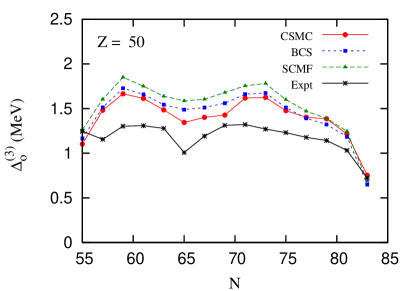
Figure 3: Pairing gaps of Sn isotopes: predictions of various theories (SCMF, BCS and CSMC) are compared with the experimental gaps.

It would be useful to know whether there are any systematic criteria for identifying nuclei for which the improved treatment of pairing has the most benefit. One criterion could be the magnitude of the error (i.e., residual) comparing the SCMF or BCS pairing gaps with their experimental values. To examine the dependence on the SCMF error we take subsets of gaps whose SCMF residual is larger (in absolute value) than some given value and calculate the rms of the subset as a function of the lower cutoff. The results are shown in Fig. 4. The rms error of the subset increases with cutoff but in the CSMC approach it does so at a lower rate than in the BCS treatment. For example, when we keep only those nuclei whose SCMF rms residual is greater than 0.5 MeV, we find that the BCS rms increases to 0.68 MeV while the CSMC rms is only 0.52 MeV, an improvement of 0.14 MeV. The inset of Fig. 4 shows the rms of the CSMC correction to the BCS residual versus the lower cutoff of the SCMF residual. This rms exhibits a gradual increase from about 0.12 MeV when all the nuclei are included to about 0.19 MeV when we include only those nuclei whose SCMF residual is greater than 0.5 MeV. Thus, there is a mild increase in the benefit derived from the exact treatment when the residual error is large.

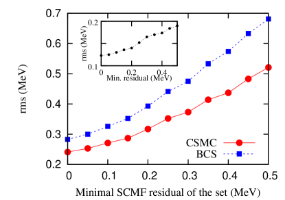
Figure 4: The rms residuals of the pairing gap in nuclei for which the absolute deviation of the SCMF pairing gap from the experimental value is greater than the value shown on the horizontal axis. The inset shows the rms of the CSMC correction to the BCS gap, the horizontal axis being the same as the main graph.

To narrow further the conditions under which an exact treatment is beneficial, we go back to the symmetries that are broken in mean field and BCS theory, namely particle-number conservation and rotational symmetry. A measure of the BCS violation of particle-number conservation is given by

$$(\Delta N)^{2}\equiv\langle(\hat{N}-\langle\hat{N}\rangle)^{2}=4\sum_{i>0}(1-v^{2}_{i})v_{i}^{2}\;,$$ (27)

where $v_{i}^{2}$ are the BCS occupation numbers. We divide the nuclei with odd number of neutrons into bins of width 1 according to their particle-number fluctuation $\Delta N$ (nuclei with $\Delta N=0$ have their own). Fig. 5 shows the rms of the residuals for the nuclei in each bin versus the midpoint of the bin. The bin with $\Delta N=0$ consists of all nuclei for which the BCS pairing has collapsed. Clearly the CSMC treatment is needed in that situation. The CSMC also gives an improvement for the bin centered at $\Delta N=3.5$ having the strongest pairing condensate. This is likely due to the too-large pairing strength $V_{0}$ required for the global BCS fit. Thus, when compared to the exact CSMC results, the BCS approximation seems to be adequate when $1\leq\Delta N\leq 3$. If we use in the BCS treatment the lower value of the CSMC interaction strength, we find the BCS performance to improve gradually with increasing $\Delta N$ and to become comparable to the CSMC performance for $\Delta N\geq 2$.

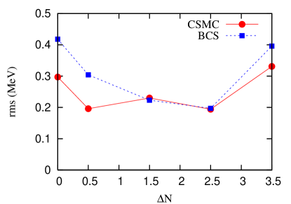
Figure 5: The rms residuals of the pairing gap as a function of particle-number fluctuation $\Delta N$ [see Eq. (27)]. The nuclei were divided into bins of width 1 according to the values of $\Delta N$ obtained from the $v$ amplitudes of the SCMF theory ($\Delta N=0$ nuclei have their own bin). The points are positioned at the center of the bins and the lines are drawn to guide the eye.

The violation of rotational symmetry in a nucleus is often characterized by the mass quadrupole deformation parameter $\beta_{2}$ defined by

$$\beta_{2}=\sqrt{\frac{\pi}{5}}\frac{Q_{0}}{A\langle r^{2}\rangle}\;,$$ (28)

where $A$, $\langle r^{2}\rangle$ and $Q_{0}$ are, respectively, the mass number, rms radius and intrinsic quadrupole moment of the nucleus. We divide the odd-$N$ nuclei into bins of width 0.1 according to their deformation $\beta_{2}$ in the SCMF treatment. The rms of the residuals are calculated for the nuclei in each bin and their values (in both BCS and CSMC) are plotted versus the bin centers in Fig. 6. We observe that there is almost no difference between the two treatments for oblate nuclei. For spherical and strongly deformed prolate nuclei, the CSMC gives a moderate improvement over BCS while for moderately deformed prolate nuclei there is a significant improvement in the CSMC method as compared with the BCS approximation.

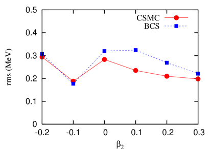
Figure 6: The rms residuals of the pairing gap as a function of deformation $\beta_{2}$ [see Eq. (28)]. The nuclei were divided into bins according to their $\beta_{2}$ value in the SCMF treatment. The points are positioned at the center of the bins, and the lines are drawn to guide the eye.

In Fig. 7 we show the average value of the ratio between the CSMC correction to the BCS correlation energy and the CSMC correlation energy, $(\delta E_{\rm CSMC}-\delta E_{\rm BCS})/\delta E_{\rm CSMC}$, versus $\Delta N$ (here $\delta E_{\rm BCS}\equiv E_{\rm HF}-E_{\rm BCS}$ and $\delta E_{\rm CSMC}\equiv E_{\rm HF}-E_{\rm CSMC}$). At $\Delta N=0$ the BCS solution collapses to the HF solution and this ratio is just $1$. We observe the above ratio to decrease monotonically versus $\Delta N$ as the BCS approximation becomes better.

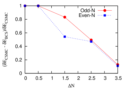
Figure 7: The ratio $(\delta E_{\rm CSMC}-\delta E_{\rm BCS})/\delta E_{\rm CSMC}$ as a function of particle-number fluctuation $\Delta N$ for nuclei with odd and even number of neutrons $N$. This ratio decreases as the BCS approximation becomes better at larger $\Delta N$. The case $\Delta N=1.5$ is a borderline case: the odd-$N$ behaves more like $\Delta N=0$ while the even-$N$ is closer to $\Delta N\gg 1$.

V Conclusion

Starting from an SCMF theory of the pairing gaps and treating pairing correlations exactly beyond the BCS approximation (with a renormalized pairing interaction strength), we found a significant improvement in the theory as measured by the rms residuals of the pairing gaps. The exact calculations were carried out by constructing a pairing Hamiltonian from the SCMF output and using the configuration space Monte Carlo (CSMC) method.

We find the improvement in the rms residuals of the pairing gaps to be most significant in nuclei for which the BCS condensate was weak, as measured by the smallness of particle-number fluctuation $\Delta N$. Based on our results, the BCS seems to be adequate if one limits the theory to nuclei for which $1\leq\Delta N\leq 3$. The artificially high value of the BCS interaction strength in a global fit leads to pairing gaps that are on average too large in nuclei with $\Delta N\geq 3$. We also found the improvement to be larger in moderately deformed ($\beta_{2}\sim 0.1-0.2$) prolate nuclei.

The total residual in the SCMF treatment of pairing gaps can be thought of as coming from two parts, the inadequacy in the mean field and the approximate treatment of pairing. Since in the CSMC method the pairing part is treated exactly, the CSMC residuals are wholly due to the inadequacy of the mean field. The rms of the residuals of the pairing gaps in the BCS treatment over their values in the CSMC treatment is then an estimate of the error involved in the BCS approximation. We find this rms value to be $\sim 0.12$ MeV (see inset of Fig. 4), and propose it as the bound on the accuracy that can be achieved in an SCMF theory that treats pairing correlations approximately.

From the computational perspective, the most notable aspect of this work is the use of the CSMC algorithm, which has not been used previously in a global survey.

Appendix A

In this Appendix we derive an estimate of the intrinsic statistical error $\sigma_{\rm in}$ based on the BCS wave function and show that it reduces to Eq. (26) in the limit of a large bandwidth $E_{c}\gg\Delta$ (assuming a uniform single-particle spectrum).

Using Eq. (25) and assuming the pair occupation $n_{i}$ to be uncorrelated, we have

$$\sigma^{2}_{\rm in}=4\sum_{i}(\varepsilon_{i}-\lambda)^{2}\sigma^{2}_{n_{i}}\;.$$ (29)

where $\sigma^{2}_{n_{i}}$ is the variance of the pair occupation $n_{i}$. To demonstrate the validity of Eq. (29), we compare in Fig. 8 the exact intrinsic variance $\sigma^{2}_{\rm in}$ (solid circles) with the r.h.s. of Eq. (29) (open circles). These quantities can be calculated directly in CSMC. The results shown are for a uniform single-particle spectrum with a level spacing of 1 MeV at half filling and a constant pairing interaction of $V_{ij}=0.3$ MeV using a time step of $\nu=0.1$. We have checked that Eq. (29) remains a good approximation for the intrinsic error in more general cases, e.g., away from half filling and for a non-uniform spectrum.

Since $n_{i}$ can take only two values $0$ or $1$, the variance $\sigma^{2}_{n_{i}}$ of a given pair occupation is completely determined by its average

$$\sigma^{2}_{n_{i}}=\bar{n}_{i}(1-\bar{n}_{i})\;.$$ (30)

Next, we use the BCS wave function to estimate

$$\bar{n}_{i}=\frac{v_{i}}{u_{i}+v_{i}}\;,$$ (31)

where $u_{i}$ and $v_{i}$ are the usual BCS amplitudes. Combining Eqs. (29), (30) and (31), we have

$$\sigma^{2}_{\rm in} =4\sum_{i}(\varepsilon_{i}-\lambda)^{2}\frac{u_{i}v_{i}}{(u_{i}+v_{i})^{2}}$$

$$=2\sum_{i}\Delta_{i}(\varepsilon_{i}-\lambda)\frac{u_{i}-v_{i}}{u_{i}+v_{i}}\;,$$ (32)

where $\Delta_{i}$ are the level-dependent BCS pairing gaps. The BCS estimate (32) for $\sigma_{\rm in}$ is shown in Fig. 8 by solid squares.

Figure 8: The intrinsic error $\sigma_{\rm in}$ as a function of $\Omega$ for a uniform single-particle spectrum with level spacing of 1 MeV and a constant pairing interaction $V_{ij}=0.3$ MeV. The exact intrinsic error (solid circles) calculated directly from CSMC (using a time step of $\nu=0.1$) is compared with the estimate of Eq. (29) with the exact $\sigma^{2}_{n_{i}}$ calculated in CSMC (open circles). The solid squares describe the BCS estimate Eq. (32) while the open squares correspond to Eq. (26). The various lines are fits describing a scaling of $\Omega^{3/2}$

.

The BCS expression (32) for the intrinsic variance can be further simplified for a uniform single-particle spectrum (in which case the gap $\Delta$ is level-independent) with a bandwidth $E_{c}\gg\Delta$. In this limit most single-particle levels satisfy $|\epsilon_{i}-\lambda|\gg\Delta$ and the BCS amplitudes can be replaced by their non-interacting values. This leads to the simple expression in Eq. (26).

In Fig. 8 we also compare the BCS estimate (32) (solid squares) with its simplified version (26) (open squares). The latter slightly overestimates the BCS expression; both underestimate the exact intrinsic variance but provide a reasonable estimate within a factor of $\sim 2$. All cases in Fig. 8 scale as $\Omega^{3/2}$ (the respective fits are shown by lines).

In the remaining part of this Appendix we show that Eq. (29) (with $\lambda$ being the chemical potential) is a good approximation, i.e., that the covariance contribution to $\sigma^{2}_{\rm in}$ in (29) is small.

Eq. (25) holds for an arbitrary parameter $\zeta$ replacing $\lambda$. Since the number of particles $N$ is conserved, we have in general

$$\sigma^{2}_{\rm in}=4\sum_{i}(\varepsilon_{i}-\zeta)^{2}\sigma^{2}_{n_{i}}+A(\zeta)\;,$$ (33)

where

$$A(\zeta)=4\sum_{i\neq j}(\varepsilon_{i}-\zeta)(\varepsilon_{j}-\zeta)\mbox{cov}(n_{i},n_{j})\;,$$ (34)

and $\mbox{cov}(n_{i},n_{j})=\overline{n_{i}n_{j}}-\bar{n}_{i}\bar{n}_{j}$ is the covariance of $n_{i}$ and $n_{j}$.

Figure 9: The variation of the fractional error $A/\sigma_{\rm in}^{2}$ (see Eq. (34)) as a function of $\zeta$ for a uniform single-particle spectrum (level spacing of 1 MeV) with $\Omega=20$ at half filling and a constant pairing interaction $V_{ij}=0.3$ MeV.

The covariance contribution to (33) vanishes for values of $\zeta$ for which $A(\zeta)=0$, a quadratic equation in $\zeta$. Using particle number conservation $2\sum_{j}n_{i}=N=2\sum_{j}\bar{n}_{i}$, we have

$$n_{i}-\bar{n}_{i}=-\sum_{j\neq i}(n_{j}-\bar{n}_{j})\;.$$ (35)

Eq. (35) implies that

$$\sigma^{2}_{n_{i}}=-\sum_{j\neq i}\mbox{cov}(n_{i},n_{j})\;.$$ (36)

Using Eq. (36), we can express the coefficients of $\zeta^{2}$ and $\zeta$ in the quadratic equation $A(\zeta)=0$ in terms of the variances alone. We then find the following two solutions

$$\zeta_{\pm}=\zeta_{0}\pm\sqrt{1+\frac{\displaystyle\sum_{i\neq j}\varepsilon_{i}\varepsilon_{j}\mbox{cov}(n_{i},n_{j})}{\zeta_{0}^{2}\sum_{i}\sigma_{n_{i}}^{2}}}\;,$$ (37)

where

$$\zeta_{0}=\frac{\displaystyle\sum_{i}\varepsilon_{i}\sigma^{2}_{n_{i}}}{\displaystyle\sum_{i}\sigma^{2}_{n_{i}}}=\frac{\displaystyle\sum_{i}\varepsilon_{i}\bar{n_{i}}(1-\bar{n_{i}})}{\displaystyle\sum_{i}\bar{n_{i}}(1-\bar{n}_{i})}$$ (38)

is the midpoint between the two solutions.

As an example we show in Fig. 9 the quantity $A/\sigma_{\rm in}^{2}$ as a function of $\zeta$ for a uniform single-particle spectrum. In general the zeros $\zeta_{\pm}$ of $A$ are not known without performing a full CSMC calculation. However, we observe that $|A/\sigma^{2}_{\rm in}|$ is rather small in the region between $\zeta_{-}$ and $\zeta_{+}$ as compared with its typical value outside this region. Thus taking $\zeta\approx\zeta_{0}$ in Eq. (33) and ignoring $A$ leads to a good approximation to $\sigma^{2}_{\rm in}$.

The sums on the r.h.s. of Eq. (38) are dominated by those levels $i$ for which $\bar{n}_{i}$ is close to $1/2$, i.e., by levels in the vicinity of the chemical potential $\lambda$. Thus we expect $\zeta_{0}$ to be in proximity to the chemical potential. We can also estimate $\zeta_{0}$ directly from Eq. (38) using the BCS expressions for $\bar{n}_{i}$ in Eq (31).

References

- (1) J. Bardeen, L.N. Cooper and J.R. Schrieffer, Phys. Rev. 108, 1175 (1957).
- (2) G. F. Bertsch, C. A. Bertulani, W. Nazarewicz, N. Schunck, and M. V. Stoitsov, Phys. Rev. C 79, 034306 (2009).
- (3) H.J. Lipkin, Ann. Phys. (NY) 9, 272 (1960); Y. Nogami, Phys. Rev. 134, B313 (1964).
- (4) J. Dobaczewski and W. Nazarewicz, Phys. Rev. C 47 2418 (1993).
- (5) M. Bender, et al., Eur. Phys. J. A. 8 59 (2000).
- (6) N. Pillet, N. Sandulescu, N. Van Giai, and J. F. Berger, Phys. Rev. C 71, 044306 (2005).
- (7) M.V. Stoitsov, J. Dobaczewski, R. Kirchner, W. Nazarewicz, and J. Terasaki, Phys. Rev. C 76, 014308 (2007).
- (8) N. Cerf and O. Martin, Phys. Rev. C 47, 2610 (1993); N. Cerf, Nucl. Phys. A564 383 (1993).
- (9) V. Zelevinsky and A. Volya, Nucl. Phys. A 752 325 (2005).
- (10) H. Molique and J. Dudek, Phys. Rev. C 56 1795 (1997).
- (11) E. Chabanat, P. Bonche, P. Haensel, J. Meyer, and F. Schaeffer, Nucl. Phys. A635, 231 (1998); 75, 121 (2003).
- (12) P. Bonche, H. Flocard, and P. H. Heenen, Comput. Phys. Commun. 171, 49 (2005).
- (13) P. Bonche, H. Flocard, P. H. Heenen, S. J. Krieger and M. S. Weiss, Nucl. Phys. A443 39 (1985).
- (14) N. Sandulescu and G. F. Bertsch, Phys. Rev. C 78, 064318 (2008).
- (15) R.W. Richardson, Phys. Rev. Lett. 3, 277 (1963); R.W. Richardson, Phys. Rev. 159, 792 (1967).
- (16) R. Capote, E. Mainegra and A. Ventura, J. Phys. G 24, 1113 (1998).
- (17) H. F. Trotter, Proc. Am. Math. Soc. 10 545 (1959).
- (18) M. Suzuki, Prog. Theor. Phys. 56, 1454 (1976); M. Suzuki, S. Miyashita, and A. Kuroda, Prog. Theor. Phys. 58, 1377 (1977).
- (19) J. E. Hirsch, D. J. Scalapino, R. L. Sugar, and R. Blankenbecler, Phys. Rev. Lett. 47, 1628 (1981).
- (20) M. V. Stoitsov, J. Dobaczewski, W. Nazarewicz and J. Terasaki, Eur. Phys. J. A 25, s01, 567 (2005).