Comparison of methods for computing the exchange energy in laterally coupled quantum dots

Abstract

We calculate the exchange energy in two dimensional laterally coupled quantum dots using Heitler-London, Hund-Mullikan and variational methods. We assess the quality of these approximations in zero and finite magnetic fields comparing against numerically exact results. We find that surprisingly, the Hund-Mullikan method does not offer any significant improvement over the much simpler Heitler-London method, whether at large or small interdot distances. Contrary to that, our variational ansatz proves substantially better. In a single dot at finite magnetic field, all approximate methods fail. This reflects the qualitative change of the single electron ground state from non-degenerate (harmonic oscillator) to highly degenerate (Landau level). However, we find that the magnetically induced failure does not occur in the most important, double-dot, regime.

I Introduction

In the last decade, a great interest in quantum dots has aroused, due to their potential use as hardware for a scalable quantum computer Loss and DiVincenzo (1998); de Sousa et al. (2001); Hu and Das Sarma (2000); Gammon (1998). In this implementation, the electron spin in quantum dots is used as the basic unit of information (qubit) Harju et al. (2002). To perform any quantum algorithm, 1-qubit and 2-qubit gates are sufficient. Any 2-qubit gate can be achieved through single qubit rotations and an adequate switching of the exchange energy, which parametrizes the spin coupling in the Heisenberg spin exchange Hamiltonian de Sousa and Das Sarma (2003); François H. and Antigoni (1998). The knowledge of the exact value of the exchange energy is important as it determines the time of the the $\sqrt{SWAP}$, a fundamental 2-qubit gate Loss and DiVincenzo (1998). The properties of the exchange energy in lateral dots have been investigated by a variety of methods: Heitler-London Pedersen et al. (2007); Burkard et al. (1999); Hu and Das Sarma (2000); de Sousa et al. (2001); Burkard et al. (2000), Hund-Mulliken Pedersen et al. (2007); Hu and Das Sarma (2000), Molecular Orbital Hu and Das Sarma (2000), Variational Kandemir (2005), Configuration Interaction Melnikov and Leburton (2006); Meller (1996); Wensauer et al. (2004), Hartree Pfannkuche et al. (1993), Hartree-Fock Hu and Das Sarma (2000); Pfannkuche et al. (1993), Hubbard model Hu and Das Sarma (2000), quantum Monte Carlo Pederiva et al. (2000) and local spin density approximation Pederiva et al. (2000); Theophilou and Papaconstantinou (2000).

This work compares several standard methods (Heitler-London, Molecular Orbital, Hund-Mulliken, Variational and the exact Configuration Interaction) to compute the exchange energy in quantum dots. We find that, with the exception of our Variational ansatz, the other standardly used extensions of the Heitler-London method do not in fact offer any real improvement. We revisit the failure of the Heitler-London method in a finite magnetic field Burkard et al. (2000). We explain the failure as due to the qualitative change of the single electron ground state from non- to highly- degenerate. As our most important result, we find that contrary to the singlet dot case, the Heitler-London method (and thus all the considered approximate methods) does not suffer the failure in the magnetic field in the double dot regime.

The article is organized as follows. In Sec. II we define the double dot model, and present the Fock-Darwin states. In Sec. III we define the approximate methods that we compare in further. In Sec. IV, we present the comparison, varying the magnetic field and the interdot distance.

II Model

We assume to have two electrons in a harmonic electrostatic potential with one (quantum helium), or two symmetrical (quantum hydrogen) minima Pfannkuche et al. (1993); Dybalski and Hawrylak (2005); Kandemir (2005); Voskoboynikov et al. (2001); Tutunculer et al. (2004). We consider the electron to be two-dimensional, as appropriate for electrically defined lateral semiconductor quantum dots de Sousa et al. (2001); Gammon (1998); François H. and Antigoni (1998); S. Kandemir (2005) in GaAs/AlGaAs heterostructure. We describe the electrons using the single band effective mass approximation Fabian et al. (2007). A constant magnetic field is applied along the growth direction (being here along the $z$-axis) S. Kandemir (2005); Creffield et al. (2000).

For the quantum hydrogen (double dot) the Hamiltonian of the $i$-th electron is given by Dybalski and Hawrylak (2005)

$$H_{d}^{(i)}=\frac{{\bf P}_{i}^{2}}{2m}+\frac{1}{2}m\omega^{2}{\rm min}\{({\bf r}_{i}-{\bf d})^{2},({\bf r}_{i}+{\bf d})^{2}\},$$ (1)

where the kinetic momentum ${\bf P}={\bf p}+e{\bf A}$ is expressed using the canonical momentum ${\bf p}=-{\rm i}\hbar{\bf\nabla}$, and the vector potential ${\bf A}=-\frac{1}{2}{\bf R}\times{\bf B}$, projected to the two dimensional plane. The magnetic field ${\bf B}=(0,0,B)$, and the position vector ${\bf R}=({\bf r},z)$, ${\bf r}=(x,y)$. The positron elementary charge is $e$, the effective mass of the electron is $m$, and $\hbar\omega$ is the confinement energy Voskoboynikov et al. (2001). The vector d defines the main dot axis with respect to the crystallographic axes.

The quantum helium (single dot) can be described setting the interdot distance to zero Dybalski and Hawrylak (2005), resulting in the Hamiltonian,

$$H_{d=0}^{(i)}=\frac{1}{2}\frac{{\bf P}_{i}^{2}}{m}+\frac{1}{2}m\omega^{2}{\bf r}_{i}^{2}\,.$$ (2)

For a system of two electrons the Hamiltonian is

$$H=H_{d}^{(1)}+H_{d}^{(2)}+H_{C}\,,$$ (3)

where $H_{C}$ is the Coulomb interaction Hamiltonian between the two electrons,

$$H_{C}=\frac{e^{2}}{4\pi\epsilon_{0}\epsilon_{r}}\frac{1}{|{\bf r}_{1}-{\bf r}_{2}|}\,,$$ (4)

where $\epsilon_{0}$ and $\epsilon_{r}$ are the vacuum and material dielectric constants, respectively. We neglect the Zeeman and spin-orbit interactions, as they are substantially smaller than the above termsStano and Fabian (2005).

In the numerical computations, we use the parameters of GaAs: $\epsilon_{r}=12.9$, $m=0.067m_{e}$ ($m_{e}$ is the free electron mass), take the confinement energy $\hbar\omega=1$ meV Szafran et al. (2004), and place the dot such that ${\bf d}=(d,0)$, that is along the x-crystallographic axis.

II.1 Fock-Darwin states

The eigenfunctions of the single dot Hamiltonian, Eq. (2), are the Fock-Darwin states de Sousa et al. (2001); S. Kandemir (2005),

$$\psi_{n\ell}^{1e}({\bf r})=C_{n\ell}r^{|\ell|}{\rm e}^{-r^{2}/(2l_{B}^{2})}L_{n}^{|\ell|}\left(\frac{r^{2}}{l_{B}^{2}}\right){\rm e}^{{\rm i}\ell\varphi}\,,$$ (5)

Here $C_{n\ell}$ is the normalization constant, $L_{n}^{\ell}$ are Laguerre polynomials, and $n$, $\ell$ are principal and orbital quantum numbers, respectively. The right hand side of Eq. (5) is expressed in polar coordinates ($r,\varphi$). The corresponding energies read,

$$E_{n,\ell}=\frac{\hbar^{2}}{l_{B}^{2}m}(2n+|\ell|+1)+\frac{eB\hbar}{2m}\ell\,,$$ (6)

where,

$$l_{B}=\left(\frac{e^{2}B^{2}}{4\hbar^{2}}+\frac{m^{2}\omega^{2}}{\hbar^{2}}\right)^{-1/4}\,,$$ (7)

is the effective confinement length.

II.2 Exchange Energy

Neglecting the Coulomb interaction, one can write the two-electron wave-function using single electron eigenstates. If the state is separable to the spinor and orbital parts, to have an antisymmetric function, orbital part must be symmetric and spinor antisymmetric, or vice versa. At low-temperature the relevant two electron Hilbert space can be restricted to comprise the two lowest orbital eigenstates of the Hamiltonian in Eq. (3). Such restricted subspace is described by an effective Hamiltonian,

$$H=\frac{J}{\hbar^{2}}{\bf S}_{1}\cdot{\bf S}_{2}\,,$$ (8)

where ${\bf S}_{1,2}=\hbar\bm{\sigma}_{1,2}/2$ are spin operators and the only parameter is $J$, the exchange energy. By this construction, the exchange energy is defined as the difference between the energy of the triplet and the singlet state Mattis (1965); Melnikov et al. (2006),

$$J=\langle\Psi_{T}|H|\Psi_{T}\rangle-\langle\Psi_{S}|H|\Psi_{S}\rangle\,,$$ (9)

where $\Psi_{S}$ and $\Psi_{T}$ are the spin singlet and triplet two-electron wave functions, respectively. These wave-functions are constructed from the single electron states (Fock-Darwin) appropriately, according to the specific method. After that, we evaluate integrals in Eq. (9) numerically, to obtain the exchange energy.

III Methods

In this section we define four approximative methods to compute the exchange energy for a system of two electrons in a coupled double dot system. They differ in the way how the two electron wave-functions, in Eq. (9), are constructed.

III.1 Heitler-London method

The Heitler-London approximation is the simplest method to calculate the exchange energy in a two electron dot Calderón et al. (2006); Hu and Das Sarma (2000). It employs the lowest Fock-Darwin state ($n=\ell=0$), displaced to the potential minima positions $\pm{\bf d}$ Burkard et al. (2000); de Sousa et al. (2001),

$$\psi_{L/R}({\bf r})=\frac{1}{l_{B}\sqrt{\pi}}\exp\left(-\frac{[(x\pm d)^{2}+y^{2}]}{2l_{B}^{2}}\pm\frac{{\rm i}edBy}{2\hbar}\right)\,.$$ (10)

From these one constructs the two-electron singlet and triplet states as,

$$\Psi_{S/T}=C_{S/T}[\psi_{L}({\bf r}_{1})\psi_{R}({\bf r}_{2})\pm\psi_{R}({\bf r}_{1})\psi_{L}({\bf r}_{2})]\chi_{S/T}\,,$$ (11)

where the singlet $\chi_{S}=\left(1/\sqrt{2}\right)\left(|\uparrow\downarrow-\downarrow\uparrow\rangle\right)$, $\chi_{T}$ is one of the three triplet states, $\left(1/\sqrt{2}\right)\left(|\uparrow\downarrow+\downarrow\uparrow\rangle\right)$, $|\uparrow\uparrow\rangle$ , $|\downarrow\downarrow\rangle$, and $C_{S/T}$ is the normalization constant.

III.2 Molecular Orbital method

The basic idea of the Molecular Orbital method is to use molecular orbitals, instead of the localized Fock-Darwin states, as the basic building blocks of the two electron wave-functions Hu and Das Sarma (2000); de Sousa et al. (2001). A Molecular orbital is the single electron eigenstate of the double dot Hamiltonian, Eq. (1). We take the following one-electron wave-functions as approximations to the lowest two molecular orbitals,

$$\psi_{\pm}({\bf r})=C_{\pm}\left[\psi_{L}({\bf r})\pm\psi_{R}({\bf r})\right]\,,$$ (12)

where $C_{\pm}$ are the normalization constants. The symmetrized combinations of the previous wave-functions form the following two electron states,

$$\begin{split}\Psi_{1}&=[\psi_{+}({\bf r}_{1})\psi_{+}({\bf r}_{2})]\chi_{S}\,,\\ \Psi_{2}&=[\psi_{-}({\bf r}_{1})\psi_{-}({\bf r}_{2})]\chi_{S}\,,\\ \Psi_{3}&=C_{3}\left[\psi_{+}({\bf r}_{1})\psi_{-}({\bf r}_{2})+\psi_{+}({\bf r}_{2})\psi_{-}({\bf r}_{1})\right]\chi_{S}\,,\\ \Psi_{4}&=C_{4}\left[\psi_{+}({\bf r}_{1})\psi_{-}({\bf r}_{2})-\psi_{+}({\bf r}_{2})\psi_{-}({\bf r}_{1})\right]\chi_{T}\,,\end{split}$$ (13)

where, again, $C_{3}$ and $C_{4}$ are normalization constants. To obtain the two electron energies, we diagonalize the Hamiltonian in Eq. (3) in the basis consisting of these four states.

III.3 Hund-Mullikan Method

In this method one expands the two electron basis used in the Heitler-London method, Eq. (11), by doubly occupied states Burkard et al. (2000), $\psi_{L}({\bf r}_{1})\psi_{L}({\bf r}_{2})$ and $\psi_{R}({\bf r}_{1})\psi_{R}({\bf r}_{2})$. It is simple to check that due to the choice of the single electron molecular orbitals, Eq. (12), such expanded basis is equivalent to the one used in the Hund-Mullikan method. It then follows that the Hund-Mullikan approximation is equivalent to the Molecular Orbital with the single electron orbitals approximated by Eq. (12).

III.4 Variational method

In the variational method one makes a guess for a trial wave-function, which depends on variational parametersKandemir (2005) . These parameters are adjusted until the energy of the trial wave-function is minimal. The resulting trial wave-function and its corresponding energy are variational method approximations to the exact wave-function and energy. Here we use the Heitler-London type of ansatz, Eq. (11), with

$$\Psi_{S,T}(D)=\Psi_{S,T}(d\rightarrow D)\,.$$ (14)

The energy is defined as the minimum over the variational parameter $D$,

$$E_{S,T}=\min\limits_{D}\langle\Psi_{S,T}(D)|H|\Psi_{S,T}(D)\rangle\,,$$ (15)

where $H$ is given by Eq. (3) and the minimization is done numerically.

III.5 Configuration Interaction Method (Exact)

The configuration interaction is a numerically exact method Wensauer et al. (2004), in which the two electron Hamiltonian is diagonalized in the basis of Slater determinants constructed from numerical single electron states in the double dot potential Baruffa et al. (2010, 2010); Wensauer et al. (2004). Typically, we use 21 single electron states, resulting in the relative error for energies of order $10^{-5}$Baruffa et al. (2010).

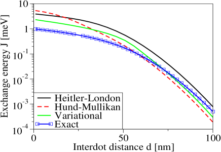
Figure 1: (Color online) Exchange energy as a function of the interdot distance for two electrons in a double dot in a zero magnetic field.

IV Results

Here we present results of the numerical calculations for the exchange energy using the methods listed in the previous. In Fig. 1 the exchange energy is plotted as a function of the interdot distance for two electrons in a double dot in zero magnetic field. We observe that for large interdot distance the exchange energy falls off exponentially, a fact that all methods reflect correctly. This suggests that, at least in principle, an efficient control of the exchange energy can be achieved by increasing the potential barrier separating the dots and/or by increasing the interdot separation. At a small interdot distance all methods differ significantly from the exact result. We note here that, despite the common belief, the Hund-Mullikan (equivalent to Molecular-Orbital) method does not offer any improvement, even at small interdot distances (strong interdot couplings). The Variational method of the form that we choose, on the other hand, proves more robust, typically cutting the error of the Heitler-London to a half.

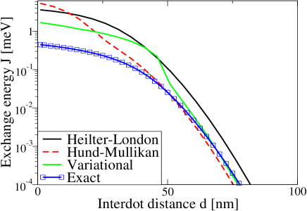
Figure 2: (Color online) Exchange energy as a function of the interdot distance for two electrons in a double dot in a finite magnetic field of $1$ Tesla.

We will see on examples that follow, that these two features are generic and we explain them below.

Figure 2 shows the exchange energy as a function of the interdot distance in a finite magnetic field $1$T. The exchange energy decreases faster than in zero magnetic field. A simple explanation follows from noting that the natural length scale is the effective confinement length $\ell_{B}$, which drops with the magnetic field, as seen from Eq. (7).

Figure  3 shows the exchange energy as a function of the magnetic field for a single dot. We can see that as the magnetic field increases, the approximative methods become increasingly off the exact results. Worse than that, except the variational method, even the trend is wrong (growth, instead of a fall-off)

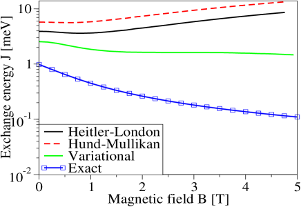
Figure 3: (Color online) Exchange energy as a function of the magnetic field for two electrons in a single dot.

To understand this failure, we plot in Fig. 4 the single electron single dot (Fock-Darwin) spectrum. One can appreciate the qualitative change between the low and high field limit. In the first, the ground state is non-degenerate, while in the second, a highly degenerate Landau level forms.

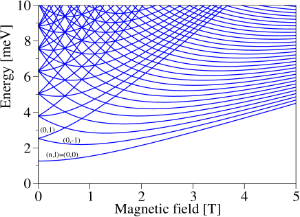
Figure 4: (Color online) Spectrum of a single electron in a single dot (Fock Darwin) as a function of the magnetic field.

The higher degeneracy, the more mixing and therefore worse results are expected for all methods based on a basis built from just a few single electron states. In other words, the effective strength of the Coulomb interaction grows with diminishing of the energy separation of the single electron states due to the magnetic field Maksym and Chakraborty (1990); Johnson and Payne (1991).

To gain further insight, we plot in Fig. 5 a comparison of the singlet and triplet energies in the Heitler-London approximation with their exact counterparts as a function of the magnetic field for a single dot.

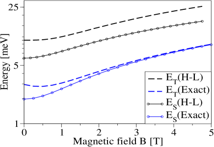
Figure 5: (Color online) Singlet and triplet energies in the Heitler-London method with their exact counterparts for a single dot.

From this we can see that both the singlet and the triplet are in the Heitler-London approximation similarly off the exact results (that is, the failure is not due to just one of them). If operating as a qubit, the double dot will be manipulated at large interdot distances.

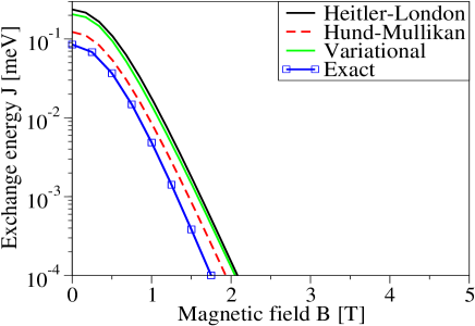
Figure 6: (Color online) Exchange energy as a function of the magnetic field for two electrons in a two-electron double dot ($d=60$ nm).

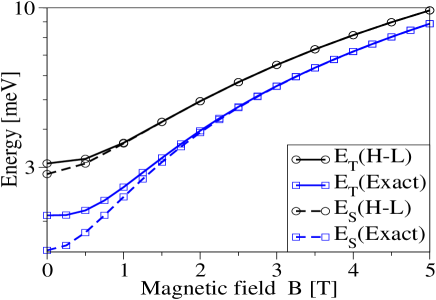
Figure 7: (Color online) Singlet and triplet energies in the Heitler-London method with their exact counterparts for double dot ($d=60$ nm).

Figure  6 shows the exchange energy in this regime. Surprisingly, the approximate methods reflect the exponential suppression of the exchange energy with the magnetic field correctly. This can be traced down to the fact that in the Heitler-London method, the exchange energy is proportional to the overlap of the localized single electron states, from Eq. (10). This is illustrated further in Fig. 7, where we plot the singlet and triplet energies in the Heitler-London approximation together with their exact values in this regime. One can see that even though the approximate values do not converge to the exact one, their errors tend to compensate. As a result, the exchange energy falls towards zero as the magnetic field is enlarged. This finding also helps to understand the previously seen trends. Namely, as seen from Eq. (13), the Molecular-Orbital approximation expands, compared to the Heitler-London, the singlet subspace only. In the resulting energy pair, the error of the singled is reduced, while the triplet is untouched. Since the exchange energy is the difference of the two energies, using the Hund-Mullikan/Molecular-Orbital is in fact detrimental compared to the Heitler-London method. The Variational method that we choose, on the other hand, treats the symmetric and antisymmetric wave-functions similarly. It is then natural to expect that their errors tend to compensate, resulting in more precise value for the exchange energy.

V Conclusions

To conclude, we studied the exchange energy in two electron single and double lateral quantum dots. We compared four approximate methods: Heitler-London, Hund-Mullikan, Molecular Orbital and Variational, with numerically exact results (the configuration interaction method). We find that, compared to the much simpler Heitler-London method, the Hund-Mullikan and Molecular Orbital methods do not offer any improvement, whether at large or small interdot distances. We explain that noting the former two methods treat the singlet and triplet wave-functions differently leading to uncompensated errors. On the other hand the variational ansatz proves robust. At finite magnetic field, all approximate methods fail. This is a consequence of the qualitative change of the single electron ground state. Finally, and most important, we find that all the approximate methods we study are free from the failure in the double dot regime.

VI Acknowledgements

We would like to thank Peter Staňo for proposing the project and for his guidance to finish it. This work was supported by the Ministry of Education, Science, Research and Sport of the Slovak Republic.

References

- Loss and DiVincenzo (1998) D. Loss and D. P. DiVincenzo, Phys. Rev. A, 57, 120 (1998).
- de Sousa et al. (2001) R. de Sousa, X. Hu, and S. Das Sarma, Phys. Rev. A, 64, 042307 (2001).
- Hu and Das Sarma (2000) X. Hu and S. Das Sarma, Phys. Rev. A, 61, 062301 (2000).
- Gammon (1998) D. Gammon, Science, 280, 225 (1998).
- Harju et al. (2002) A. Harju, S. Siljamäki, and R. M. Nieminen, Phys. Rev. Lett., 88, 226804 (2002).
- de Sousa and Das Sarma (2003) R. de Sousa and S. Das Sarma, Phys. Rev. B, 68, 155330 (2003).
- François H. and Antigoni (1998) J. François H. and A. Antigoni, Science, 282, 1429 (1998).
- Pedersen et al. (2007) J. Pedersen, C. Flindt, N. A. Mortensen, and A.-P. Jauho, Phys. Rev. B, 76, 125323 (2007).
- Burkard et al. (1999) G. Burkard, D. Loss, and D. P. DiVincenzo, Phys. Rev. B, 59, 2070 (1999).
- Burkard et al. (2000) G. Burkard, G. Seelig, and D. Loss, Phys. Rev. B, 62, 2581 (2000).
- Kandemir (2005) B. S. Kandemir, Phys. Rev. B, 72, 165350 (2005).
- Melnikov and Leburton (2006) D. V. Melnikov and J.-P. Leburton, Phys. Rev. B, 73, 155301 (2006).
- Meller (1996) J. Meller, New computational algorithms based on the Configuration Interaction method, Ph.D. thesis, Nicholas Copernicus Universityin Torun (1996).
- Wensauer et al. (2004) A. Wensauer, M. Korkusinski, and P. Hawrylak, Solid State Communications, 130, 115 (2004).
- Pfannkuche et al. (1993) D. Pfannkuche, V. Gudmundsson, and P. A. Maksym, Phys. Rev. B, 47, 2244 (1993).
- Pederiva et al. (2000) F. Pederiva, C. J. Umrigar, and E. Lipparini, Phys. Rev. B, 62, 8120 (2000).
- Theophilou and Papaconstantinou (2000) A. K. Theophilou and P. G. Papaconstantinou, Phys. Rev. A, 61, 022502 (2000).
- Dybalski and Hawrylak (2005) W. Dybalski and P. Hawrylak, Phys. Rev. B, 72, 205432 (2005).
- Voskoboynikov et al. (2001) O. Voskoboynikov, C. P. Lee, and O. Tretyak, Phys. Rev. B, 63, 165306 (2001).
- Tutunculer et al. (2004) H. Tutunculer, R. Koc, and E. Olgar, Journal of Physics A: Mathematical and General, 37, 11431 (2004).
- S. Kandemir (2005) B. S. Kandemir, Journal of Mathematical Physics (2005).
- Fabian et al. (2007) J. Fabian, A. Matos-Abiague, C. Ertler, P. Stano, and I. Zutic, Acta Physica Slovaca, 57, 565 (2007).
- Creffield et al. (2000) C. E. Creffield, J. H. Jefferson, S. Sarkar, and D. L. J. Tipton, Phys. Rev. B, 62, 7249 (2000).
- Stano and Fabian (2005) P. Stano and J. Fabian, Phys. Rev. B, 72, 155410 (2005).
- Szafran et al. (2004) B. Szafran, F. M. Peeters, and S. Bednarek, Phys. Rev. B, 70, 205318 (2004).
- Mattis (1965) D. Mattis, The Theory of Magnetism, Mattis (Harper and Row, 1965).
- Melnikov et al. (2006) D. V. Melnikov, J.-P. Leburton, A. Taha, and N. Sobh, Phys. Rev. B, 74, 041309 (2006).
- Calderón et al. (2006) M. J. Calderón, B. Koiller, and S. Das Sarma, Phys. Rev. B, 74, 045310 (2006).
- Baruffa et al. (2010) F. Baruffa, P. Stano, and J. Fabian, Phys. Rev. Lett., 104, 126401 (2010a).
- Baruffa et al. (2010) F. Baruffa, P. Stano, and J. Fabian, Phys. Rev. B, 82, 045311 (2010b).
- Maksym and Chakraborty (1990) P. A. Maksym and T. Chakraborty, Phys. Rev. Lett., 65, 108 (1990).
- Johnson and Payne (1991) N. F. Johnson and M. C. Payne, Phys. Rev. Lett., 67, 1157 (1991).