Ground states of unfrustrated spin Hamiltonians satisfy an area law

Abstract

We show that ground states of unfrustrated quantum spin-$1\!/2$ systems on general lattices satisfy an entanglement area law, provided that the Hamiltonian can be decomposed into nearest-neighbor interaction terms which have entangled excited states. The ground state manifold can be efficiently described as the image of a low-dimensional subspace of low Schmidt measure, under an efficiently contractible tree-tensor network. This structure gives rise to the possibility of efficiently simulating the complete ground space (which is in general degenerate). We briefly discuss “non-generic” cases, including highly degenerate interactions with product eigenbases, using a relationship to percolation theory. We finally assess the possibility of using such tree tensor networks to simulate almost frustration-free spin models.

I Introduction

An important insight in the study of quantum many-body systems is related to the observation that common states that naturally occur do not quite exhaust the entire Hilbert space available to them, but instead a much smaller subspace. This insight is at the heart of powerful numerical methods that have been devised in recent years. Ideas such as the density-matrix renormalization group approach, and new ideas that allow for the simulation of higher-dimensional quantum lattice models Review ; Scholl ; 2d , work exactly because they model well quantum states that in a certain sense have little entanglement. More precisely, the states which are tractible by these approaches satisfy what is called an area law Review ; Wilczek ; Bombelli ; Srednicki ; Harmonic ; Latorre ; Area1 ; Area2 ; Jin ; Cardy ; Fermi1 ; Fermi2 ; Fermi3 ; Hastings ; Masanes , so the entropy of a subregion scales at most as the boundary area of that region (for a review, see Ref. Review ). For practical purposes, and in particular for 1D systems, these methods in particular give accurate accounts of ground state properties.

Now, not all ground states of local quantum lattice models can be efficiently approximated. This holds even true for 1D chains: indeed, one can construct models for which approximating the ground state energy is provably NP-hard NPH — albeit using a fairly sophisticated construction involinvg large local dimensions Power . An important feature of these constructions is that the difficulty of their solution appears to be strongly related to whether the system is frustrated or not. This suggests that whether or not the system is frustrated is another criterion for whether a quantum lattice model should be considered “easy” or “hard”, in addition to its ground states having “a lot” or “little” entanglement. This intuition that frustrated systems should be hard to simulate is indeed true for classical systems, where the frustrated or glassy models are the hard ones to describe. For quantum systems, there is evidence that the situation should be more complex Shor .

In this work, we explore a class of models where the intuition of frustration-free models being easy to solve holds true. Building upon work in Ref. Bravyi06 and in Ref. OurPRL , for a natural class of two-local Hamiltonians acting on spin-$1/2$ particles (simply “spins” henceforth), we show that ground states can be reduced to a completely characterized and low-dimensional subspace, and then re-constructed by identifying the ground state-space of each interaction of the Hamiltonian term-by-term. Specifically, the ground space is the image of a symmetric subspace under an explicitly constructible, and efficiently contractible, tensor network. It follows that the ground states satisfy an area law, and hence contain little entanglement in the above sense. This generalizes recent results regarding the existence of states which have little entanglement in the ground-state manifolds of such Hamiltonians NoGoMBQC . We discuss how to efficiently simulate the ground state manifold, and suggest how this could be used to simulate “almost” frustration-free quantum lattice models.

II Preliminaries

II.1 Frustration-free Hamiltonians and area laws

We consider spin-$1/2$ Hamiltonians on a lattice. The lattice is described by some graph, the vertex set of which we denote by $V$. Naturally, the Hamiltonian will be local, or more specifically include only nearest-neighbor interaction terms. We represent the Hamiltonian as

$$H\;=\!\sum_{\left\{a,b\right\}\subseteq V}\!h_{a,b}$$ (1)

for some terms $h_{a,b}$ acting on pairs of spins in the lattice described by $V$. By rescaling, we may without loss of generality require that the ground state energy of each interaction term $h_{a,b}$ is zero. We wish to describe properties of the ground state manifold $M$ of such Hamiltonians, given the list of the individual two-spin terms $h_{a,b}$ as input. An important class of Hamiltonians are those which are frustration-free (or unfrustrated), for which each ground state vector $\left\lvert\Phi\right\rangle\mspace{-1.5mu}\in M$ is also a ground state of the individual coupling terms: i.e. for which

$$h_{a,b}\left\lvert\Phi\right\rangle\mspace{-1.5mu}=0$$ (2)

holds for all $h_{a,b}$ and all $|\Phi\rangle\in M$. The actual ground state $\rho$ is the maximally mixed state over $M$, and so is mixed unless the ground state manifold $M$ is non-degenerate.

Our main results pertain to frustration-free spin Hamiltonians as above, with the further constraint that each term $h_{a,b}$ has at least one entangled excited state. In Section VI, we show that the ground states $\rho$ of such Hamiltonians satisfy an area law Review ; Wilczek ; Bombelli ; Srednicki ; Harmonic ; Latorre ; Area1 ; Area2 ; Jin ; Cardy ; Fermi1 ; Fermi2 ; Fermi3 ; Hastings ; Masanes : that is, for a contiguous region of spins $A\subseteq V$, the entanglement of formation. If the ground state is non-degenerate and hence pure, the entanglement of formation is nothing but the usual entanglement entropy. of the ground state satisfies

$$E_{F}(\rho)\leqslant C|\partial A|$$ (3)

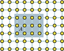
for $C>0$ constant, where $|\partial A|$ is the “boundary area” (i.e. the number of edges in the interaction graph of $H$, which are incident to both $A$ and $V\smallsetminus A$): see Fig. 1. The entanglement of formation is the largest asymptotically continuous entanglement monotone, so this also implies an entanglement area law for e.g. the distillable entanglement. Thus, ground states of frustration-free Hamiltonians contain little entanglement.

Figure 1: The entanglement scales at most as the boundary area $|\partial A|$ of a distinguished region $A$ in some lattice, here a cubic lattice, with tighter bounds for special cases.

This follows as a consequence of the fact that the ground-state manifold is the image of the symmetric subspace on $n$ spins (for some $n$ bounded above by the number of spins of the Hamiltonian) under an efficiently simulatable, and explicitly constructible, tree-tensor network. We show this in Section V, in which we demonstrate how this allows us to efficiently simulate the ground space of the spin models we consider. For the cases where we have a tree tensor network with a single top root, the problem considered here may be viewed as exactly the converse problem to the one discussed in Ref. Giov .

Our result of an analytical area law complements results on area laws in harmonic bosonic systems Harmonic ; Area1 ; Area2 , fermionic Fermi1 ; Fermi2 ; Fermi3 on cubic lattice and general gapped models in one-dimensional quantum chains Hastings . For a comprehensive review on area laws — and on implications on the simulatability of quantum many-body systems — see Ref. Review .

II.2 Quantum 2-sat problem

The arguments behind our analysis builds upon and extends the ideas of Ref. Bravyi06 , which defined the problem of quantum satisfiability, and presented Bravyi’s algorithm for quantum ${2}$-sat. We describe here the connection between this problem and frustration in spin Hamiltonians.

quantum ${2}$-sat is the quantum analogue of the “classical” 2-sat problem on boolean formulae. The latter asks when there exists an assignment of boolean variables $x_{1},\ldots,x_{n}$ which simultaneously “satisfy” a collection of constraints on pairs of those variables. This problem is efficiently solvable APT79 ; in contrast, the similar problem 3-sat (in which constraints apply to triples of variables) is NP-complete Karp72 . In quantum ${2}$-sat, individual clauses on boolean variables are replaced by projectors $p_{a,b}$ with

$$p^{2}_{a,b}=p_{a,b}$$ (4)

on pairs of spins: an instance of quantum ${2}$-sat is satisfiable if there is a vector which is a zero eigenvector of each projector simultaneously.

For an instance of quantum ${2}$-sat, determining whether there exist such simultaneous zero eigenvectors is equivalent to determining whether the Hamiltonian obtained by summing the projectors is unfrustrated. Conversely, the problem of determining when a $2$-local spin Hamiltonian $H$ is frustration-free may be reduced to quantum ${2}$-sat, by rescaling the terms of the Hamiltonian $H$ so that each term $h_{a,b}$ has a minimal eigenvalue of $0$, and replacing each rescaled term $h_{a,b}$ with the projector $p_{a,b}$ onto $\operatorname{img}(h_{a,b})$. By construction, such a substituation does not affect the ground space of the terms. Thus, solving quantum ${2}$-sat is equivalent to determining whether a $2$-local spin Hamiltonian is frustration-free.

Recently, random instances of quantum ${k}$-sat with rank-$1$ projectors Footnote have been studied for $k\geqslant 2$, delineating the “boundary” of frustration in $k$-local spin Hamiltonians in terms of the density of interactions kQSat ; RandomQSat ; BravyiQSat ; Zittartz . We instead extend the findings of Ref. Bravyi06 for $k=2$, remarking on implications for simulating the ground space manifold in frustration-free Hamiltonians. In Section III, we review Bravyi’s algorithm for quantum ${2}$-sat, in order to demonstrate important features of the reductions involved when they are applied to unfrustrated Hamiltonians satisfying natural constraints.

III Reduction tools for frustration-free Hamiltonians

Bravyi’s algorithm for quantum ${2}$-sat Bravyi06 efficiently demonstrates the satisfiability of an instance of quantum ${2}$-sat by a sequence of reductions of Hamiltonians, yielding a homogeneous instance (in which all projectors have rank $1$), and then verifying the satisfiability of these instances. We may similarly use Bravyi’s algorithm to detect frustration in $2$-local spin Hamiltonians, and consider the features of these Hamiltonian reductions when applied to particular classes of frustration-free Hamiltonians.

Throughout the following, we admit representations of Hamiltonians $H^{\prime}$ with non-zero single spin terms $h_{a}$,

$$H^{\prime}\;=\!\sum_{\left\{a,b\right\}\subseteq V}\!\!h_{a,b}\;\;+\;\;\sum_{a\in V}h_{a}\;,$$ (5)

and again describe $H^{\prime}$ as unfrustrated if there exists a joint ground state with eigenvalue zero of all terms (including the single-spin terms $h_{a}$).

III.1 Reductions by isometries

Condensing the analysis of Ref. Bravyi06 , we consider a reduction for $2$-local Hamiltonians $H$ to Hamiltonians $H^{\prime}$ on fewer spins, provided that $H$ contains only positive semidefinite terms which have non-trivial kernels. Throughout, we denote $\mathbb{C}^{2}$ by $\mathcal{H}_{2}$.

III.1.1 Two-spin isometric contractions

Consider a Hamiltonian term $h_{u,v}$ of rank $2$ or $3$. If $H$ is frustration-free, $h_{u,v}$ fixes a subspace of $\mathcal{H}_{2}^{\otimes\left\{u,v\right\}}$ of dimension at most $2$, over which the reduced state $\rho_{u,v}$ of a state vector $\left\lvert\Phi\right\rangle\mspace{-1.5mu}\in\ker(H)$ must be a mixture. We describe this reduced state by an encoding of one spin into two. Let $\left\{\left\lvert\psi_{0}\right\rangle\mspace{-1.5mu},\left\lvert\psi_{1}\right\rangle\mspace{-1.5mu},\left\lvert\psi_{2}\right\rangle\mspace{-1.5mu},\left\lvert\psi_{3}\right\rangle\mspace{-1.5mu}\right\}$ be an orthonormal basis for $\mathcal{H}_{2}\otimes\mathcal{H}_{2}$ such that

$$\ker(h_{u,v})\subseteq\operatorname{span}\left\{\left\lvert\psi_{0}\right\rangle\mspace{-1.5mu},\left\lvert\psi_{1}\right\rangle\mspace{-1.5mu}\right\}.$$ (6)

Define an isometry $U_{u:u,v}:\mathcal{H}_{2}^{\otimes\left\{u\right\}}\!\longrightarrow\!\mathcal{H}_{2}^{\otimes\left\{u,v\right\}}$ such that

$$\sum_{x\in\left\{0,1\right\}}\!\!\alpha_{x}\left\lvert x\right\rangle\mspace{-1.5mu}_{u}\quad\mapstochar\longrightarrow \;\;\sum_{x\in\left\{0,1\right\}}\!\!\alpha_{x}\left\lvert\psi_{x}\right\rangle\mspace{-1.5mu}_{u,v}\;.$$ (7)

This is an isometric reduction, similar to those in a tree tensor network or a MERA ansatz MERA . By construction, the support of the reduced state $\rho_{u,v}$ lies in $\operatorname{img}(U_{u:uv})$. We may then define a Hamiltonian

$$H^{\prime}=U_{u:u,v}^{\dagger}HU_{u:u,v}$$ (8)

on the subsystem $V^{\prime}=V\smallsetminus\left\{v\right\}$, where the spin $v$ is essentially deleted; any state vector $\left\lvert\Phi\right\rangle\mspace{-1.5mu}\in\ker(H)$ then has the form

$$\left\lvert\Phi\right\rangle\mspace{-1.5mu}=U_{u:uv}\left\lvert\Phi^{\prime}\right\rangle\mspace{-1.5mu},\qquad\left\lvert\Phi^{\prime}\right\rangle\mspace{-1.5mu}\in\ker(H^{\prime}).$$ (9)

We may express $H^{\prime}$ as a sum of terms

$$h^{\prime}_{a,b}=U_{u:u,v}^{\dagger}h_{a,b}U_{u:u,v},\quad h^{\prime}_{a}=U^{\dagger}_{u:u,v}h^{\prime}_{a}U_{u:u,v}.$$ (10)

(In the case that $h$ is of rank $3$, these will include a non-zero single spin operator $h^{\prime}_{u,v}$ which acts on $u$ alone.) If $H$ contains non-zero terms $h_{a,u}$ and $h_{a,v}$, we obtain two terms $h^{\prime}_{a,u}=U^{\dagger}_{u:u,v}h_{a,u}U_{u:u,v}$ and $h^{\prime}_{a,v}=U^{\dagger}_{u:u,v}h_{a,v}U_{u:u,v}$ in the Hamiltonian $H$, which both act on the spins $u$ and $a$. We sum these to obtain a combined term

$$\bar{h}^{\prime}_{a,u}=h^{\prime}_{a,u}+h^{\prime}_{a,v}$$ (11)

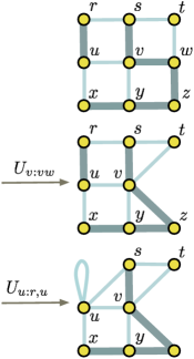
in the reduced Hamiltonian, which may be of higher rank than either $h^{\prime}_{a,u}$ or $h^{\prime}_{a,v}$. (We similarly accumulate any single-spin contributions $h^{\prime}_{u}$ and $h^{\prime}_{v}$ which may arise from single-spin terms $h_{u}$ and $h_{v}$ in $H$.) Fig. 2 illustrates the effect of multiple reductions on the interaction graph of the Hamiltonian.

Figure 2: Illustration of transformations of the interaction graph of a Hamiltonian $H$ by two-spin isometries. Darker, thicker edges represent interaction terms $h_{a,b}$ of rank $2$ or $3$, which may be eliminated by contraction (corresponding to a reduction $H\mapstochar\rightarrow U_{a:ab}^{\dagger}HU_{a:ab}$). In the case of an interaction term with $\operatorname{rank}(h_{r,u})=3$ as illustrated above, a single spin operator (represented above by a loop) is produced on the contracted vertex.

For example: Consider an anti-ferromagnetic four-spin Hamiltonian, with interactions

$$h_{j,k}\;=\;\tfrac{1}{2}\sigma_{x}^{(j)}\sigma_{x}^{(k)}\;+\;\tfrac{1}{2}\sigma_{y}^{(j)}\sigma_{y}^{(k)}$$ (12)

on a four-spin cycle with interacting pairs $(1,2)$, $(2,3)$, $(3,4)$, and $(4,1)$. Here we denote

$$\sigma_{x}\;= \;\left[\;\begin{matrix}0&1\\ 1&0\end{matrix}\;\right]\;=\;\left\lvert 1\right\rangle\mspace{-1.5mu}\mspace{-1.5mu}\left\langle 0\right\rvert+\left\lvert 0\right\rangle\mspace{-1.5mu}\mspace{-1.5mu}\left\langle 1\right\rvert,$$ (13a)

$$\sigma_{y}\;= \;\left[\;\begin{matrix}0&\!-i\\ i&0\end{matrix}\;\right]\;=\;i\left\lvert 1\right\rangle\mspace{-1.5mu}\mspace{-1.5mu}\left\langle 0\right\rvert-i\left\lvert 0\right\rangle\mspace{-1.5mu}\mspace{-1.5mu}\left\langle 1\right\rvert.$$ (13b)

Rescaling the interactions to have ground energy zero (and taking these for the $h_{j,k}$ instead) gives us

$$h_{j,k}\;=\;\left\lvert 0,0\right\rangle\mspace{-1.5mu}\mspace{-1.5mu}\left\langle 0,0\right\rvert_{j,k}+\left\lvert 1,1\right\rangle\mspace{-1.5mu}\mspace{-1.5mu}\left\langle 1,1\right\rvert_{j,k}\;.$$ (14)

The kernel of this operator is clearly spanned by $\left\lvert 0,1\right\rangle\mspace{-1.5mu}$ and $\left\lvert 1,0\right\rangle\mspace{-1.5mu}$. We may consider the effect of contracting spins $3$ and $4$ into a renormalized spin, using the isometry

$$R_{3:3,4}=\big{(}\left\lvert 0\right\rangle\mspace{-1.5mu}_{3}\otimes\left\lvert 1\right\rangle\mspace{-1.5mu}_{4}\big{)}\mspace{-1.5mu}\left\langle 0\right\rvert_{3}+\big{(}\left\lvert 1\right\rangle\mspace{-1.5mu}_{3}\otimes\left\lvert 0\right\rangle\mspace{-1.5mu}_{4}\big{)}\mspace{-1.5mu}\left\langle 1\right\rvert_{3}\;.$$ (15)

By construction, we have $R_{3:3,4}^{\dagger}h_{3,4}R_{3:3,4}=0$; and as $\left\{1,2\right\}$ is disjoint from $\left\{3,4\right\}$, we have $h^{\prime}_{1,2}=R_{3:3,4}^{\dagger}h_{1,2}R_{3:3,4}=h_{1,2}$. We compute the renormalized terms $h^{\prime}_{2,3}$ and $h^{\prime}_{4,1}$ as

$$h^{\prime}_{2,3}\;= \;R_{3:3,4}^{\dagger}\Big{(}\left\lvert 0,0\right\rangle\mspace{-1.5mu}\mspace{-1.5mu}\left\langle 0,0\right\rvert_{2,3}\otimes\openone_{4}+\left\lvert 1,1\right\rangle\mspace{-1.5mu}\mspace{-1.5mu}\left\langle 1,1\right\rvert_{2,3}\otimes\openone_{4}\Big{)}R_{3:3,4}$$

$$= \;\left\lvert 0,0\right\rangle\mspace{-1.5mu}\mspace{-1.5mu}\left\langle 0,0\right\rvert_{2,3}+\left\lvert 1,1\right\rangle\mspace{-1.5mu}\mspace{-1.5mu}\left\langle 1,1\right\rvert_{2,3}\;,$$ (16a)

$$h^{\prime}_{4,1}\;= \;R_{3:3,4}^{\dagger}\Big{(}\openone_{3}\otimes\left\lvert 0,0\right\rangle\mspace{-1.5mu}\mspace{-1.5mu}\left\langle 0,0\right\rvert_{4,1}+\openone_{3}\otimes\left\lvert 1,1\right\rangle\mspace{-1.5mu}\mspace{-1.5mu}\left\langle 1,1\right\rvert_{4,1}\Big{)}R_{3:3,4}$$

$$= \;\left\lvert 1,0\right\rangle\mspace{-1.5mu}\mspace{-1.5mu}\left\langle 1,0\right\rvert_{3,1}+\left\lvert 0,1\right\rangle\mspace{-1.5mu}\mspace{-1.5mu}\left\langle 0,1\right\rvert_{3,1}\;;$$ (16b)

up to rescaling, the resulting renormalized Hamiltonian is then

$$H^{\prime}=R_{3:3,4}^{\dagger}HR_{3:3,4}\sim \;\tfrac{1}{2}\Big{(}\big{[}\sigma_{x}^{(1)}\sigma_{x}^{(2)}+\sigma_{y}^{(1)}\sigma_{y}^{(2)}\big{]}$$

$$\;\;+\;\big{[}\sigma_{x}^{(2)}\sigma_{x}^{(3)}+\sigma_{y}^{(2)}\sigma_{y}^{(3)}\big{]}$$

$$\;\;-\;\big{[}\sigma_{x}^{(3)}\sigma_{x}^{(1)}+\sigma_{y}^{(3)}\sigma_{y}^{(1)}\big{]}\Big{)}\;,$$ (17)

with a ferromagnetic coupling between the site $1$ and the renormalized site $3$. Arbitrary rank-2 or rank-3 interactions may be contracted similarly.

III.1.2 Single-spin deletions

For a $2$-local Hamiltonian $H$ containing non-zero single-spin operators $h_{v}$ (e.g., such as may arise from the preceding reduction), any state vector $\left\lvert\Phi\right\rangle\mspace{-1.5mu}\in\ker(H)$ must be factorizable into a single-spin pure state vector $\left\lvert\psi\right\rangle\mspace{-1.5mu}\in\ker(h_{v})$ acting on $v$, and some state of the remaining spins. If the operator $h_{v}$ has full rank, it follows $\left\lvert\psi\right\rangle\mspace{-1.5mu}=\text{\boldmath$0$}$, so that $H$ has trivial kernel. Otherwise, $\left\lvert\psi\right\rangle\mspace{-1.5mu}$ may be taken to be a unit vector spanning the kernel of $h_{v}$, and we may form a Hamiltonian

$$H^{\prime}=\bigl{(}\mspace{-1.5mu}\left\langle\psi\right\rvert_{v}\otimes\mathbbm{1}\bigr{)}H\bigl{(}\left\lvert\psi\right\rangle\mspace{-1.5mu}_{v}\otimes\mathbbm{1}\bigr{)}$$ (18)

on the subsystem $V^{\prime}=V\smallsetminus\left\{v\right\}$, consisting of a sum of terms $h^{\prime}_{a}=h_{a}$ acting on individual spins $a\neq v$, and terms

$$h^{\prime}_{a,b}=\bigl{(}\mspace{-1.5mu}\left\langle\psi\right\rvert_{v}\otimes\mathbbm{1}\bigr{)}h_{a,b}\bigl{(}\left\lvert\psi\right\rangle\mspace{-1.5mu}_{v}\otimes\mathbbm{1}\bigr{)},$$ (19)

acting on pairs of spins $\left\{a,b\right\}\subseteq V$. In the latter case, if $v\in\left\{a,b\right\}$, then $h^{\prime}_{a,b}$ will be an operator acting on a single spin; otherwise, we have $h^{\prime}_{a,b}=h_{a,b}$. Again, in the case of single-spin terms $h^{\prime}_{a,b}$ acting on a spin $a$, if there was a term $h_{a}$ present in $H$, we may accumulate these into a term $\bar{h}^{\prime}_{a}=h_{a}+h^{\prime}_{a,b}$.

We may again describe $H^{\prime}$ using an isometric reduction in this case: if we define $P_{v}=\left\lvert\psi_{v}\right\rangle\mspace{-1.5mu}\otimes\mathbbm{1}_{V^{\prime}}$, then $P_{v}$ is an isometry whose image contains any state vector $\left\lvert\Phi\right\rangle\mspace{-1.5mu}\in\ker(H)$. We may then rewrite Eq. 18 as

$$H^{\prime}=P_{v}^{\dagger}HP_{v}.$$ (20)

expressing it in a form more explicitly similar to Eq. 8.

III.1.3 Remarks on these reductions

The reductions above correspond to the reductions presented in Ref. Bravyi06 for instances of quantum ${2}$-sat which contain two-spin operators of rank greater than $1$. This allows us to reduce quantum ${2}$-sat to the special case of “homogeneous” instances (in which all terms have rank $1$).

The key feature of both reductions above is that the kernels of $H$ and $H^{\prime}$ are related by isometries, and so have the same dimension. If the Hamiltonian $H^{\prime}$ has any terms of full rank (acting on either one or two spins), it follows that the Hamiltonian $H^{\prime}$ has trivial kernel; then the same holds for $H$ as well. If we do not encounter any full-rank terms, each reduc- tion produces a Hamiltonian acting on one fewer spins, even- tually yielding a “homogeneous” Hamiltonian (extending the terminology of Ref. Bravyi06 to Hamiltonians in general, including those with single-spin terms of rank 1).

The choice of the reduction at each stage does not matter, in the following sense. As long as we have a Hamiltonian containing two-spin terms of rank at least $2$, and which does not contain full-rank terms, we may extend any sequence of reductions to one which terminates with a Hamiltonian $\tilde{H}$ which is either homogeneous or contains a full-rank term. In the latter case, the original Hamiltonian has trivial kernel, and is therefore frustrated; otherwise, we obtain a “homogeneous” Hamiltonian whose kernel may be mapped to that of the original Hamiltonain $H$ by a sequence of known isometries. If we can solve the homogeneous case, we may then choose the reductions according to whichever criteria are convenient.

Note that this reduction process, from an input Hamiltonian $H$ to a homogeneous Hamiltonian, amounts to a tree tensor network of isometries (albeit applied to a vector subspace): from a temporal top layer defined by a Hamiltonian containing only terms of rank $1$, one constructs the ground space of the full Hamiltonian $H$ by sequential applications of isometries with a simple topology. We develop this observation further, and remark on implications for simulating the ground space of $H$, in Section V. Note also that for a one-dimensional quantum chain and a sequential contraction, this construction gives rise to a sequential preparation of a quantum state and hence to a matrix-product state of small bond dimension.

III.2 The homogeneous case

Given a homogeneous Hamiltonian $H^{\prime}$ (containing only terms of rank 1) acting on some system $V^{\prime}$, consider a collection of vectors $\left\lvert\beta_{a,b}\right\rangle\mspace{-1.5mu}\in\mathcal{H}_{2}^{\otimes\left\{a,b\right\}}$ such that

$$h_{a,b}=\left\lvert\beta_{a,b}\right\rangle\mspace{-1.5mu}\mspace{-1.5mu}\left\langle\beta_{a,b}\right\rvert\;.$$ (21)

We interpret each two-spin Hamiltonian term $h^{\prime}_{a,b}$ as a constraint on the corresponding two-spin marginal state $\rho_{a,b}$ of a state $\left\lvert\Phi\right\rangle\mspace{-1.5mu}\in\ker(H)$, and attempt to obtain additional constraints on pairs of spins $a,b\in V^{\prime}$ by combinations of the constraints which are already known. Ref. Bravyi06 shows that if $\left\lvert\Phi\right\rangle\mspace{-1.5mu}$ lies in the kernel of $\mspace{-1.5mu}\left\langle\beta_{a,b}\right\rvert$ and $\mspace{-1.5mu}\left\langle\beta_{b,c}\right\rvert$ acting on the corresponding spins, it also lies in the kernel of the functional

$$\mspace{-1.5mu}\left\langle\beta^{\prime}_{a,c}\right\rvert=\bigl{(}\mspace{-1.5mu}\left\langle\beta_{a,b}\right\rvert\otimes\mspace{-1.5mu}\left\langle\beta_{b,c}\right\rvert\bigr{)}\bigl{(}\mathbbm{1}\otimes\left\lvert\Psi^{-}\right\rangle\mspace{-1.5mu}\otimes\mathbbm{1}\bigr{)}$$ (22)

acting on the spins $a$ and $c$, where $\left\lvert\Psi^{-}\right\rangle\mspace{-1.5mu}\propto\left\lvert 0\right\rangle\mspace{-1.5mu}\left\lvert 1\right\rangle\mspace{-1.5mu}-\left\lvert 1\right\rangle\mspace{-1.5mu}\left\lvert 0\right\rangle\mspace{-1.5mu}$ is the two-spin antisymmetric state vector. We call such a constraint $\mspace{-1.5mu}\left\langle\beta^{\prime}_{a,c}\right\rvert$ an “induced” constraint, and use the term induction of constraints to refer to the operation on $\mspace{-1.5mu}\left\langle\beta_{a,b}\right\rvert$ and $\mspace{-1.5mu}\left\langle\beta_{b,c}\right\rvert$ which gives rise to $\mspace{-1.5mu}\left\langle\beta^{\prime}_{a,c}\right\rvert$ in Eq. 22, up to a scalar factor.

For each induced constraint $\mspace{-1.5mu}\left\langle\beta^{\prime}_{u,v}\right\rvert$ on a pair of spins $u,v$, we may add a term

$$\tilde{h}_{u,v}=\left\lvert\beta^{\prime}_{u,v}\right\rangle\mspace{-1.5mu}\mspace{-1.5mu}\left\langle\beta^{\prime}_{u,v}\right\rvert$$ (23)

to the Hamiltonian $H^{\prime}$, obtaining a Hamiltonian $\tilde{H}$ which (by construction) has the same kernel as $H^{\prime}$. If $H^{\prime}$ already contains a term $h_{u,v}$ which is not colinear to the induced term $\tilde{h}_{u,v}$, these may be accumulated into a term $\bar{h}_{u,v}$ whose rank is at least $2$, and one may apply a two-spin contraction as described in Section III.1. Otherwise, we may induce further constraints from the terms of $\tilde{H}$, until we obtain a complete homogeneous Hamiltonian $H_{c}$: a Hamiltonian in which the two-spin constraints $\mspace{-1.5mu}\left\langle\beta_{u,v}\right\rvert$ are closed under constraint-induction.

By inducing constraints on pairs of spins, possibly performing two-spin contractions as in Section III.1 when we obtain terms of rank $2$ or more, we may efficiently obtain a complete homogeneous Hamiltonian $H_{c}$ from a frustration-free, $2$-local Hamiltonian $H$. Furthermore, Ref. Bravyi06 shows that a complete homogeneous Hamiltonian $H_{c}$ acting on at least one spin (and which lacks single-spin operators Footnote2 ) has a ground space which contains product states. Thus, for homogeneous Hamiltonians $H$, we may either efficiently determine that it is frustrated, or efficiently obtain a Hamiltonian which is closed under constraint-induction. In the latter case, we may construct product states in the kernel of $H$ by selecting states for each spin consistent with the two-spin constraints Footnote3 .

IV Unfrustrated Natural Hamiltonians

We now present results concerning the ground state manifold of a “physical” class of $2$-local spin Hamiltonians. We will say that a Hamiltonian $H$ is natural if it is $2$-local, contains no isolated subsystems, and each term $h_{a,b}$ (acting on $\mathcal{H}_{2}\otimes\mathcal{H}_{2}$) has at least one entangled excited state (i.e., there exists an entangled state orthogonal to the ground state manifold of $h_{a,b}$). Without loss of generality, we may further require that the ground energy of each term in $H$ is zero. This is a natural assumption that typical physical interactions will satisfy: for instance, ferromagnetic or anti-ferromagnetic Ising interactions (which have excited eigenstates $\left\lvert 0\right\rangle\mspace{-1.5mu}\left\lvert 1\right\rangle\mspace{-1.5mu}-\left\lvert 1\right\rangle\mspace{-1.5mu}\left\lvert 0\right\rangle\mspace{-1.5mu}$ and $\left\lvert 0\right\rangle\mspace{-1.5mu}\left\lvert 0\right\rangle\mspace{-1.5mu}+\left\lvert 1\right\rangle\mspace{-1.5mu}\left\lvert 1\right\rangle\mspace{-1.5mu}$ respectively), ferromagnetic or anti-ferromagnetic XXX models (which also have those respective eigenstates), or indeed any interaction which is inequivalent to either $\operatorname{diag}(0,0,E_{a},E_{b})$ or $\operatorname{diag}(0,E_{a},0,E_{b})$ up to rescaling and a choice of basis for each spin.

Using the reductions of Section III.1, we show strong bounds on the dimension of the ground space of an unfrustrated natural Hamiltonian on spins. This will allow us in Section V to describe a scheme for efficiently simulating the ground space of frustration-free natural Hamiltonians, and in Section VI to demonstrate that the ground states of such Hamiltonians satisfy an entanglement area law.

IV.1 Ground-spaces of unfrustrated, natural, homogeneous Hamiltonians

We now present an extension of the analysis of Ref. Bravyi06 for homogeneous and complete Hamiltonians $H_{c}$ (acting on a set $V_{c}$ of spins), to examine the ground-state manifold of $H_{c}$ in the case that $H_{c}$ is also natural. We show, using techniques similar to those used in Ref. (RandomQSat, , Section III A), that the ground space of such a Hamiltonian is equivalent to the symmetric subspace $\operatorname{Symm}(\mathcal{H}_{2}^{\otimes V_{c}})\subseteq\mathcal{H}_{2}^{\otimes V_{c}}$, up to some efficiently constructible choice of invertible operations on each spin. As we may reduce more general Hamiltonians, i.e. having terms of rank $2$ or $3$ (extending beyond those Hamiltonians considered in Ref. RandomQSat ) to homogeneous natural Hamiltonians via the reductions of Section III.1, these results yield important consequences for natural frustration-free Hamiltonians in general.

Consider a Hamiltonian $H_{c}$ acting on $V_{c}$, where $H_{c}$ has no single-spin terms. Because the two-spin constraints de- scribed by the terms of $H_{c}$ are closed under the induction of constraints (as described by Eq. 22), and as there are no isolated subsystems, it is easy to show that every pair of spins is acted on by a non-zero term in $H_{c}$. For such a Hamiltonian, the excited states $\left\lvert\beta_{a,b}\right\rangle\mspace{-1.5mu}$ for the terms $h_{a,b}$ in $H_{c}$ are entangled states. We may then construct a family of operators $\left\{L_{v}\right\}_{v\in V_{c}}\subseteq\mathrm{GL}(2)$ such that

$$\mspace{-1.5mu}\left\langle\beta_{u,v}\right\rvert\;\propto\;\mspace{-1.5mu}\left\langle\Psi^{-}\right\rvert_{u,v}\bigl{(}L_{u}\otimes L_{v}\bigr{)}$$ (24)

for each pair of spins $u,v$, where $\left\lvert\Psi^{-}\right\rangle\mspace{-1.5mu}$ is again the two-spin antisymmetric state vector. For instance, one may fix $L_{a}=\mathbbm{1}$ for an arbitrarily chosen spin $a\in V_{c}$, and determine linear operators $L_{v}$ satisfying Eq. 24 for each $v\in V_{c}$ and operator $\mspace{-1.5mu}\left\langle\beta_{a,v}\right\rvert$. Any such choice of operators $\left\{L_{v}\right\}_{v\in V_{c}}$ satisfies Eq. 24 for all $u,v$, which follows from the closure of the constraints $\mspace{-1.5mu}\left\langle\beta_{u,v}\right\rvert$ under induction:

$$\mspace{-1.5mu}\left\langle\beta_{u,v}\right\rvert\;\propto \;\;\bigl{(}\mspace{-1.5mu}\left\langle\beta_{ua}\right\rvert\otimes\mspace{-1.5mu}\left\langle\beta_{a,v}\right\rvert\bigr{)}\bigl{(}\mathbbm{1}\otimes\left\lvert\Psi^{-}\right\rangle\mspace{-1.5mu}\otimes\mathbbm{1}\bigr{)}$$

$$\propto \;\;\bigl{(}\mspace{-1.5mu}\left\langle\Psi^{-}\right\rvert\otimes\mspace{-1.5mu}\left\langle\Psi^{-}\right\rvert\bigr{)}\bigl{(}L_{u}\otimes\left\lvert\Psi^{-}\right\rangle\mspace{-1.5mu}\otimes L_{v}\bigr{)}$$

$$\propto \;\;\mspace{-1.5mu}\left\langle\Psi^{-}\right\rvert\bigl{(}L_{u}\otimes L_{v}\bigr{)}.$$ (25)

We define scalars $\lambda_{u,v}\neq 0$ such that $\mspace{-1.5mu}\left\langle\beta_{u,v}\right\rvert=\lambda_{u,v}\mspace{-1.5mu}\left\langle\Psi^{-}\right\rvert\bigl{(}L_{u}\otimes L_{v}\bigr{)}$ for each $u,v\in V_{c}$, and let $T=(\bigotimes_{v\in V_{c}}L_{v})\mathchoice{{}^{-1}}{{}^{-1}}{{}^{\kern 0.3014pt\text{--}1}}{{}^{\kern 0.3014pt\text{--}1}}$: we then have

$$\mspace{-5.0mu}\bigl{(}\mspace{-1.5mu}\left\langle\beta_{u,v}\right\rvert\otimes\mathbbm{1}\bigr{)}T\;= \mspace{-1.5mu}\left\langle\Psi^{-}\right\rvert_{u,v}\otimes T_{\overline{u,v}}\;,$$ (26a)

where we define $$T_{\overline{u,v}}$$ by

$$T_{\overline{u,v}}\;\;= \;\;\lambda_{u,v}\!\bigotimes_{w\neq u,v}L_{w}^{-1}.$$ (26b)

As the operators $T_{\overline{u,v}}$ have full rank, the operator $\big{(}\mspace{-1.5mu}\left\langle\beta_{u,v}\right\rvert\otimes\mathbbm{1}\big{)}T$ then has the same kernel as $\mspace{-1.5mu}\left\langle\Psi^{-}\right\rvert_{u,v}$ , which is the $+1$-eigenspace of the swap operator acting on $u$ and $v$. It follows that the kernel of the Hamiltonian

$$T^{\dagger}H_{c}T\;= \;\sum_{u,v\in V_{c}}T^{\dagger}\bigl{(}\left\lvert\beta_{u,v}\right\rangle\mspace{-1.5mu}\mspace{-1.5mu}\left\langle\beta_{u,v}\right\rvert\otimes\mathbbm{1}\bigr{)}T$$

$$= \;\sum_{u,v\in V_{c}}\left\lvert\Psi^{-}\right\rangle\mspace{-1.5mu}\mspace{-1.5mu}\left\langle\Psi^{-}\right\rvert_{u,v}\otimes T_{\overline{u,v}}^{\dagger}\>\!T_{\overline{u,v}}^{\phantom{\dagger}}$$ (27)

is the symmetric subspace $\operatorname{Symm}(\mathcal{H}_{2}^{\otimes V_{c}})$; this corresponds to the result of (RandomQSat, , Section III A).

We remark on some important properties of $\operatorname{Symm}(\mathcal{H}_{2}^{\otimes n_{c}})$, where $n_{c}=|V_{c}|$. This subspace is spanned by uniform superpositions $\left\lvert W_{k}\right\rangle\mspace{-1.5mu}$ of the standard basis states having Hamming weight $0\leqslant k\leqslant n_{c}$,

$$\left\lvert W_{k}\right\rangle\mspace{-1.5mu}\;\;\;\propto\!\sum_{\begin{subarray}{c}x\in\left\{0,1\right\}^{n_{c}}\\ \!\!\!\|x\|_{1}=k\end{subarray}}\left\lvert x\right\rangle\mspace{-1.5mu}\;;$$ (28)

thus $\dim\operatorname{Symm}(\mathcal{H}_{2}^{\otimes n_{c}})=n_{c}+1$. This subspace may also be spanned by product state vectors $\left\lvert\alpha_{0}\right\rangle\mspace{-1.5mu}^{\otimes n_{c}}\!,\ldots,\left\lvert\alpha_{n_{c}}\right\rangle\mspace{-1.5mu}^{\otimes n_{c}}$ for any set of $n_{c}+1$ pairwise independent state vectors $\left\lvert\alpha_{j}\right\rangle\mspace{-1.5mu}\in\mathcal{H}_{2}$. Thus, any natural Hamiltonian $H_{c}$ which is also complete and homogenous has a ground space of dimension $n_{c}+1$, and can be spanned by a family of classically efficiently simulatable state vectors

$$\left\lvert\Phi_{j}\right\rangle\mspace{-1.5mu}\;= \;\bigotimes_{v\in V_{c}}\bigl{(}L_{v}\left\lvert\alpha_{j}\right\rangle\mspace{-1.5mu}\bigr{)},$$ (29)

for some choice of pair-wise independent single-spin state vectors $\left\lvert\alpha_{0}\right\rangle\mspace{-1.5mu},\ldots,\left\lvert\alpha_{n_{c}}\right\rangle\mspace{-1.5mu}\in\mathcal{H}_{2}$; we use this fact in Section V. Note that if even this efficient method should be too computationally costly for very large systems, one can also Monte-Carlo sample from the ground state manifold in this way.

IV.2 Preservation of natural Hamiltonians under reductions

A key feature of natural Hamiltonians (defined on page IV) is that the class of frustration-free natural Hamiltonians on spins is preserved by the two-spin contractions described in Eq. 8. This implies that the reductions of Section III.1 map the ground-state manifold of an unfrustrated natural Hamiltonian $H$ provided as input to that of a complete, homogeneous, natural Hamiltonian; we may then apply the results of the preceding section to describe the ground-state manifold of $H$.

Consider an isometry $U_{u:u,v}:\mathcal{H}_{2}^{\otimes\left\{u\right\}}\longrightarrow\mathcal{H}_{2}^{\otimes\left\{u,v\right\}}$ derived from a two-spin Hamiltonian term $h_{u,v}$ as described in Section III.1.1. We may show that for any term $h_{a,u}$ in $H$, the corresponding term $h^{\prime}_{a,u}=U_{u:u,v}^{\dagger}h_{a,u}U_{u:u,v}$ in the reduced Hamiltonian $H^{\prime}=U_{u:u,v}^{\dagger}HU_{u:u,v}$ has an entangled excited state if the same holds for $h_{a,u}$. We require the following two lemmas, whose proofs we defer to Appendix A:

Lemma 1 (Product states).

For two-spin state vectors $\left\lvert\psi\right\rangle\mspace{-1.5mu}$ and $\left\lvert\phi\right\rangle\mspace{-1.5mu}$, we have $\big{(}\mspace{-1.5mu}\left\langle\psi\right\rvert\otimes\mathbbm{1}\big{)}\big{(}\mathbbm{1}\otimes\left\lvert\phi\right\rangle\mspace{-1.5mu}\big{)}=0$ only if both $\left\lvert\psi\right\rangle\mspace{-1.5mu}$ and $\left\lvert\phi\right\rangle\mspace{-1.5mu}$ are product states.

Lemma 2 (Product operators).

Let $U:\mathcal{H}_{2}\longrightarrow\mathcal{H}_{2}\otimes\mathcal{H}_{2}$ be an isometry which is not a product operator. Let $\eta\geqslant 0$ be an operator on two spins, and $\eta^{\prime}=\big{(}U^{\dagger}\otimes\mathbbm{1}_{2})(\mathbbm{1}_{2}\otimes\eta)(U\otimes\mathbbm{1}_{2})$. If $\eta^{\prime}$ is not of full rank, then $\eta^{\prime}$ is a product operator if and only if $\eta$ is a product operator.

We show that frustration-free natural Hamiltonians are preserved by the reductions of Section III.1.1 as follows. Let $H$ be a natural $2$-local Hamiltonian, and $h_{u,v}$ be a two-spin term in $H$. Define

$$U_{u:u,v}\;=\;\left\lvert\psi_{0}\right\rangle\mspace{-1.5mu}\mspace{-1.5mu}\left\langle 0\right\rvert+\left\lvert\psi_{1}\right\rangle\mspace{-1.5mu}\mspace{-1.5mu}\left\langle 1\right\rvert$$ (30)

for orthonormal two-spin state vectors $\left\lvert\psi_{0}\right\rangle\mspace{-1.5mu},\left\lvert\psi_{1}\right\rangle\mspace{-1.5mu}$ whose span contains $\ker(h_{u,v})$; we require that $\left\lvert\psi_{1}\right\rangle\mspace{-1.5mu}$ be entangled, which ensures that $U_{u:u,v}$ is not a product operator. Consider the terms $h^{\prime}_{a,b}=U_{u:u,v}^{\dagger}h_{a,b}U_{u:u,v}$ which occur in the Hamiltonian $H^{\prime}=U_{u:u,v}^{\dagger}HU_{u:u,v}$. For any two-spin operator $h_{v,a}$ acting on $v$ and some other spin $a$, the fact that $h_{v,a}$ has an entangled excited state implies in particular that it is not a product operator. Thus, $h^{\prime}_{v,a}$ is a product operator only if it has full rank. If $H$ is frustration-free, $h^{\prime}_{v,a}$ cannot have full rank; then $h^{\prime}_{v,a}$ is not a product operator, and in particular it will have entangled excited states. As $h^{\prime}_{a,b}=h_{a,b}$ when $a,b\notin\left\{u,v\right\}$, it follows that $H^{\prime}$ is a natural Hamiltonian; and as $H^{\prime}$ has a kernel of the same dimension as $H$, it is frustration-free as well.

We may strengthen this result, to show that if $H$ is natural and frustration-free, and also contains no two-spin terms of rank $1$, then the same is true of $H^{\prime}=U_{u:u,v}^{\dagger}HU_{u:u,v}$ as well. For any two-spin term $h_{v,a}$ acting on $v$ with rank at least $2$, consider states $\left\lvert\varphi_{0}\right\rangle\mspace{-1.5mu},\left\lvert\varphi_{1}\right\rangle\mspace{-1.5mu}\in\operatorname{img}(h_{v,a})$ such that $\left\lvert\varphi_{0}\right\rangle\mspace{-1.5mu}=\left\lvert\alpha\right\rangle\mspace{-1.5mu}\left\lvert\beta\right\rangle\mspace{-1.5mu}$ is a product state and $\left\lvert\varphi_{1}\right\rangle\mspace{-1.5mu}$ is entangled; Any subspace of $\mathcal{H}_{2}\otimes\mathcal{H}_{2}$ of dimension at least $2$, such as $\operatorname{img}(h_{u,v})$, contains a product state vector $\left\lvert\varphi_{0}\right\rangle\mspace{-1.5mu}$; the existence of $\left\lvert\varphi_{1}\right\rangle\mspace{-1.5mu}$ is guaranteed by the definition of a natural Hamiltonian (compare also Ref. Tarrach ). and choose real parameters $\lambda_{0},\lambda_{1}>0$ such that

$$h_{v,a}-\lambda_{0}\left\lvert\varphi_{0}\right\rangle\mspace{-1.5mu}\mspace{-1.5mu}\left\langle\varphi_{0}\right\rvert-\lambda_{1}\left\lvert\varphi_{1}\right\rangle\mspace{-1.5mu}\mspace{-1.5mu}\left\langle\varphi_{1}\right\rvert\;\geqslant\;0.$$ (31)

Let $\eta_{k}=\left\lvert\varphi_{k}\right\rangle\mspace{-1.5mu}\mspace{-1.5mu}\left\langle\varphi_{k}\right\rvert$ for $k\in\left\{0,1\right\}$, and consider the images $\eta^{\prime}_{k}$ under contraction by $U_{u:u,v}$ :

$$\eta^{\prime}_{k}\;= \;\;U_{u:u,v}^{\dagger}\eta_{k}U_{u:u,v}$$

$$= \;\;\sum_{j,\ell}\bigl{(}\left\lvert j\right\rangle\mspace{-1.5mu}\mspace{-1.5mu}\left\langle\psi_{j}\right\rvert\otimes\mathbbm{1}\bigr{)}\bigl{(}\mathbbm{1}\otimes\eta_{k}\bigr{)}\bigl{(}\left\lvert\psi_{\ell}\right\rangle\mspace{-1.5mu}\mspace{-1.5mu}\left\langle\ell\right\rvert\otimes\mathbbm{1}\bigr{)}$$

$$= \;\;\sum_{j,\ell}\left\lvert j\right\rangle\mspace{-1.5mu}\mspace{-1.5mu}\left\langle\ell\right\rvert\otimes M_{j,k}M_{\ell,k}^{\dagger}\;,$$ (32)

where we define $M_{j,k}=\big{(}\mspace{-1.5mu}\left\langle\psi_{j}\right\rvert\otimes\mathbbm{1}\big{)}\big{(}\mathbbm{1}\otimes\left\lvert\varphi_{k}\right\rangle\mspace{-1.5mu}\big{)}$. By Lemma 1, we have $M_{j,k}=0$ only if both $\left\lvert\psi_{j}\right\rangle\mspace{-1.5mu}$ and $\left\lvert\varphi_{k}\right\rangle\mspace{-1.5mu}$ are product operators; this implies that the operators $M_{1,k}$ in particular are non-zero, so that $\eta^{\prime}_{k}\neq 0$ for any $k$. Note that

$$h^{\prime}_{v,a}\;= \;U_{u:u,v}^{\dagger}h_{v,a}U_{u:u,v}$$

$$\geqslant \;\lambda_{0}U_{u:u,v}^{\dagger}\eta_{0}U_{u:u,v}\;+\;\lambda_{1}U_{u:u,v}^{\dagger}\eta_{1}U_{u:u,v}$$

$$= \;\lambda_{0}\eta^{\prime}_{0}\;+\;\lambda_{1}\eta^{\prime}_{1}\;;$$ (33)

because $H^{\prime}$ has a non-trivial kernel, $h^{\prime}_{v,a}$ has rank at most $3$, in which case neither operator $\eta^{\prime}_{k}$ has full rank. By Lemma 2, $\eta^{\prime}_{1}$ is not a product operator; as $\eta^{\prime}_{0}$ is a product operator, these operators are linearly independent. Then, $\lambda_{0}\eta^{\prime}_{0}\;+\;\lambda_{1}\eta^{\prime}_{1}$ has rank at least $2$; by Eq. IV.2, the same is true of $h^{\prime}_{v,a}$. If all of the terms in $H$ have rank $2$ or higher, the same then holds for $H^{\prime}$ as well.

Thus, if we apply the reductions of Section III.1 to an initial Hamiltonian which is both natural and frustration-free, the resulting Hamiltonians will also be natural and frustration free. Furthermore, if $H$ contains no terms of rank $1$, then neither will the reduced Hamiltonians. Because the process of inducing constraints described in Section III.2 also preserves the property of each term $h_{a,b}$ having entangled excited states, these invariants ensure that initial Hamiltonians with these properties (natural and frustation-free, and possibly containing no terms of rank $1$) may be reduced to homogeneous and complete Hamiltonians which have these same properties. We may then apply the results of Section IV.1 to these reduced Hamiltonians.

Figure 3: A simple tree tensor network.

V Simulating ground spaces of frustration-free natural Hamiltonians

Building on the results of Section IV, we now show how the reductions of Section III.1 may be used to obtain a procedure for simulating states from the ground-state manifold of frustration-free natural Hamiltonians $H$.

V.1 Tree tensor networks and matrix-product states

As we noted on page III.1.3, implicit in the reductions of Section III.1 is that the isometric reduction from general Hamiltonians to homogeneous instances has the form of a tree-tensor network. Thus, simulating the ground state manifold of any unfrustrated $2$-local Hamiltonian on spins may be reduced to that of a complete homogeneous Hamiltonian acting on a smaller system. In this section, we sketch this reduction.

For any unfrustrated $2$-local Hamiltonian $H$ on $n$ spins, we may apply two-spin reductions as described in Section III.1 until we obtain a homogeneous instance without single-spin terms. We then attempt to induce additional constraints via Eq. 22, and apply further two-spin reductions if we obtain terms of rank $2$ or $3$. If $H$ is frustration-free, this process will ultimately terminate in a complete homogeneous Hamiltonian $H_{c}$ on a subset $V_{c}\subseteq V$.

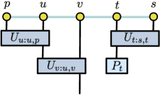
Consider the tensor network $T$ which performs the complete reduction as above; we describe $T$ in reverse order, as introducing new spins to represent a unitary embedding of $\ker(H_{c})$ into $\ker(H)$. The various “spin contraction” isometries $U_{u:u,v}$ as in Eq. 7 each have a single input-index and two output indices; the “spin deletion” isometries $P_{v}$ have no input indices at all. These are applied sequentially, giving rise to an acyclic directed network. As the in-degree of each tensor is at most $1$, it follows that the network contains no cycles at all (neither directed nor undirected): the output indices of each tensor represent spins whose state depends on only a single spin at the input. Put another way: any spin $v$ which is introduced by an isometry $U_{u:u,v}$ may be considered a “daughter spin” of a unique parent $U$, which imposes a tree-like hierarchy on the tensor network $T$, as illustrated in Fig. 3. Strictly speaking, the quantum circuit or tree tensor network will have the structure of a forest graph, which is a graph which may have more than one connected component, each of which are trees.

The roots of each tree are spins $u$ which are either prepared by an isometry $P_{u}$ derived from the removal of single-spin terms, or which correspond to free indices at the input of the tensor network $T$.

In the case that $H$ is non-degenerate, the resulting tensor network will (by that fact) simply be a tree-tensor network with no free input indices. Conversely, if the input Hamiltonian $H$ is degenerate, there will necessarily be free input indices, representing a domain consisting of a state space of dimension at least $2$. In the latter case, the tensor network $T$ will yield ground states of the original unfrustrated Hamiltonian $H$ if and only if it operates on a state $\left\lvert\varphi\right\rangle\mspace{-1.5mu}\in\ker(H_{c})$ at the input, where $H_{c}$ is the complete homogeneous instance obtained by the Hamiltonian reductions. Thus, if one may efficiently simulate states from the ground space of such a Hamiltonian, we may apply the network $T$ to simulate the ground space of the original Hamiltonian $H$.

V.2 Efficiently simulating ground spaces of unfrustrated natural Hamiltonians

Tensor networks $T$ with free input indices, and with a tree-like structure such as described above, can be efficiently simulated over inputs with low Schmidt measure SM , as follows.

For any observable $\Omega$ acting on $m$ spins, one may evaluate $\left\langle\Omega\right\rangle_{H}$ for the maximally mixed state over the ground-state manifold of $H$ by computing the expectation $\left\langle T^{\dagger}\Omega T\right\rangle_{\smash{H_{c}}}$ over the ground-state manifold of the complete homogeneous Hamiltonian $H_{c}$ obtained as described in Section III. As the tensor $T$ has tree-stucture, the observable $T^{\dagger}\Omega T$ also acts on at most $m$ spins. If we can obtain an orthonormal basis for $\ker(H_{c})$ which may be succinctly described in terms of product states, we may evaluate expectation values of $T^{\dagger}\Omega T$ with respect to $m$-fold products of single spin states.

As we noted in Section IV.1, $\ker(H_{c})$ can be spanned by a collection of $n_{c}+1$ product vectors (where $n_{c}$ is the number of spins on which $H_{c}$ acts). Let $\left\lvert\Phi^{\prime}_{0}\right\rangle\mspace{-1.5mu},\left\lvert\Phi^{\prime}_{1}\right\rangle\mspace{-1.5mu},\ldots,\left\lvert\Phi^{\prime}_{n_{c}}\right\rangle\mspace{-1.5mu}\in\ker(H_{c})$ be a collection of independent product vectors,

$$\left\lvert\Phi^{\prime}_{j}\right\rangle\mspace{-1.5mu}\;=\;\left\lvert\varphi_{j,1}\right\rangle\mspace{-1.5mu}\otimes\left\lvert\varphi_{j,2}\right\rangle\mspace{-1.5mu}\otimes\cdots\otimes\left\lvert\varphi_{j,n_{c}}\right\rangle\mspace{-1.5mu}\;.$$ (34)

We may efficiently compute a projection of $\Omega_{c}$ onto $\ker(H_{c})$ by performing a suitable transformation of the matrix

$$W(\Omega_{c})\;= \;\sum_{j,k=0}^{n_{c}}\left\lvert j\right\rangle\mspace{-1.5mu}\mspace{-1.5mu}\left\langle\Phi^{\prime}_{j}\right\rvert\Omega_{c}\left\lvert\Phi^{\prime}_{k}\right\rangle\mspace{-1.5mu}\mspace{-1.5mu}\left\langle k\right\rvert\;,$$ (35)

as follows. The operator $W(\openone)$ in particular is positive definite; we thus have $W(\openone)=U\Delta U^{\dagger}$ for some unitary $U$ unitary and positive diagonal matrix $\Delta$. It is not difficult to show that

$$\Delta^{-1/2}U^{\dagger}\sum_{j=0}^{n_{c}}\left\lvert j\right\rangle\mspace{-1.5mu}\mspace{-1.5mu}\left\langle\Phi^{\prime}_{j}\right\rvert\;=\;\sum_{j=0}^{n_{c}}\left\lvert j\right\rangle\mspace{-1.5mu}\mspace{-1.5mu}\left\langle\Phi_{j}\right\rvert\;,$$ (36)

for some orthonormal basis $\left\lvert\Phi_{0}\right\rangle\mspace{-1.5mu},\ldots,\left\lvert\Phi_{n_{c}}\right\rangle\mspace{-1.5mu}$ of $\ker(H_{c})$, by taking the product of the above operator with its adjoint. Thus, the restriction of $\Omega_{c}$ to $\ker(H_{c})$ with respect to the basis of states $\left\lvert\Phi_{j}\right\rangle\mspace{-1.5mu}$ may be computed as

$$\bar{\Omega}\;= \;\Delta^{-1/2}U^{\dagger}W(\Omega_{c})U\Delta^{-1/2}.$$ (37)

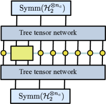
By considering operators $\Omega_{c}=T^{\dagger}\Omega T$, this allows us to compute the restriction of operators to the ground-space of $H_{U}$: see Fig. 4.

Figure 4: Schematic diagram showing the isometric decomposition for efficient simulating the ground state manifold. A local Hamiltonian term supported on two sites is marked yellow.

We may thus efficiently estimate such observables with respect to ground-states of $H_{U}$: for constant $m$, the required inner products may be calculated as (sums of) scalar products of at most $n_{c}$ inner products over vector spaces of bounded dimension. To evaltuate the value of $\Omega$ with respect to ground states of the input Hamiltonian $H$, it suffices to analyse the polynomially-sized operator $\bar{\Omega}$ representing the action of $\Omega$ on the ground-state manifold.

VI Entanglement bounds for ground states of frustration-free natural Hamiltonians

The fact that the reductions of Section III.1 preserve the class of natural Hamiltonians (as defined on page IV) allow us also to make more global statements about ground states for frustration-free Hamiltonians, again by reduction to the complete homogeneous case described in Section IV.1. In this section, considering frustration-free natural Hamiltonians $H$, we demonstrate an area law for the entanglement possible in a ground state of $H$ between any subsystem $A\subseteq V$ and its environment $V\smallsetminus A$. We also consider some very general cases in which still stronger upper bounds on the entanglement may be obtained.

VI.1 Area law for frustration-free natural Hamiltonians

We consider first the case where $A$ is a contiguous subsystem (i.e. for which there is a path between any pair of spins in $A$, following edges in the interaction graph of the Hamiltonian $H$), and subsequently generalize the observation in this case to arbitrary subsystems $A$. We first decompose

$$H\;=\;H_{A}+H_{B}+H_{A,B}\;,$$ (38)

for $B=V\smallsetminus A$, and where $H_{A}$ and $H_{B}$ contain all terms internal to $A$ and $B$, respectively. We then apply the reductions of Section III.1 to the subsystem $A$. That is, we perform two-spin contractions as described in Section III.1.1 for any two-spin terms in $H_{A}$ of rank $2$ or $3$, and perform spin-deletions as described in Section III.1.2 for any single-spin terms in $H_{A}$. Performing the constraint-induction process of Eq. 22 — again on the terms acting on $A$ alone — and then reducing further reductions as necessary, we eventually obtain a Hamiltonian $\tilde{H}$ of the form

$$\tilde{H}\;=\;\tilde{H}_{\tilde{A}}+H_{B}+\tilde{H}_{\tilde{A},B}\;,$$ (39)

where $\tilde{A}\subseteq A$ is the set of spins remaining after the reduction process, and where $\tilde{H}_{\tilde{A}}$ is a homogeneous and complete Hamiltonian. The Hamiltonians $\tilde{H}_{\tilde{A}}$ and $\tilde{H}_{\tilde{A},B}$ contain the terms derived from $H_{A}$ and $H_{A,B}$ respectively by the reduction process. In other words, we perform a complete tree tensor reduction on the subsystem $A$, until we obtain a Hamiltonian whose restriction to $A$ is homogeneous and complete. As $\dim\ker(\tilde{H})=\dim\ker(H)>0$, we have $\ker(\tilde{H}_{\tilde{A}})>0$ and $\ker(H_{B})>0$ as well; in particular, $\ker(\tilde{H})\subseteq\ker(\tilde{H}_{\tilde{A}})$, so that $\tilde{H}_{\tilde{A}}$ is frustation-free. Because $\ker(\tilde{H})\subseteq\ker(H_{B})$ as well, we then have

$$\ker(\tilde{H})\subseteq\ker(\tilde{H}_{\tilde{A}})\otimes\ker(H_{B})$$ (40)

taking the restrictions of $\tilde{H}_{\tilde{A}}$ and $H_{B}$ to their respective subsystems $\tilde{A}$ and $B$. Let $\tilde{n}=|\tilde{A}|$: as $\tilde{H}_{\tilde{A}}$ is also homogeneous and complete, it has kernel of dimension $\tilde{n}+1$ by Section IV.1.

In the case where $A$ contains multiple components $A_{1},A_{2},\ldots,A_{k}$ with respect to the interaction graph of $H$ (where each $A_{j}$ is disconnected from the others but connected internally), we may perform the Hamiltonian reductions of Section III.1 to each component independently. We may further decompose the Hamiltonian $\tilde{H}_{\tilde{A}}$ obtained in Eq. 39 as

$$\tilde{H}_{\tilde{A}}\;=\;\tilde{H}_{\tilde{A}_{1}}+\cdots+\tilde{H}_{\tilde{A}_{k}},\;\;\;\text{where $\tilde{A}_{j}=\tilde{A}\,\cap\,A_{j}$}.$$ (41)

As $\tilde{H}_{\tilde{A}}$ is unfrustrated, each of the sub-Hamiltonians $\tilde{H}_{\tilde{A}_{j}}$ is unfrustrated as well, in which case we may write

$$\ker(\tilde{H}_{\tilde{A}})\;\subseteq\;\ker(\tilde{H}_{\tilde{A}_{1}})\otimes\cdots\otimes\ker(\tilde{H}_{\tilde{A}_{k}}),$$ (42)

similarly to Eq. 40. Then, the dimension of $\ker(H_{\tilde{A}})$ is bounded by the product of $\dim\ker(\tilde{H}_{\tilde{A}_{j}})=\tilde{n}_{j}+1$ for each subsystem, where $\tilde{n}_{j}=\left\lvert\smash{\tilde{A}}_{j}\right\rvert$. Let $\alpha_{j}$ be the number of spins in $A_{j}$ which are adjacent in the spin lattice to spins in $B$, and let $\tilde{\alpha}_{j}\leqslant\alpha_{j}$ be the number of such spins in $\tilde{A}_{j}$. For any $H$ with nearest neighbor interactions on a lattice in finitely many dimensions (in the graph theoretical sense), there exist scalars $c,K>0$ such that

$$\alpha_{j}\geqslant Kn_{j}^{c}$$ (43)

for each subsystem $A_{j}$. We may then bound on the dimension of $\ker(\tilde{H}_{\tilde{A}})$ in terms of these “boundary spins” as

$$\log(\dim \ker(\tilde{H}_{\tilde{A}}))\;\leqslant\;\sum_{j=1}^{k}\log(\dim\;\!\ker(\tilde{H}_{\tilde{A}_{j}}))$$

$$\leqslant \;\sum_{j=1}^{k}\log(\tilde{n}_{j}+1)\;\leqslant\;\sum_{j=1}^{k}\tilde{n}_{j}^{c}\;\leqslant\;\frac{\alpha}{K},$$ (44)

where $\alpha=\alpha_{1}+\cdots+\alpha_{k}$ is the number of spins in $A$ adjacent to elements of $B$.

From this bound on $\dim\ker(\tilde{H}_{\tilde{A}})$, it follows that any pure state $\left\lvert\Phi\right\rangle\mspace{-1.5mu}$ in the ground space of $\tilde{H}$ has Schmidt measure SM at most ${\alpha}/{K}$ across the partition $\tilde{A}+B$, and so can support at most this many e-bits of entanglement between $\tilde{A}$ and $B$. Because any state vector $\left\lvert\Psi\right\rangle\mspace{-1.5mu}\in\ker(H)$ can be obtained from some vector $\left\lvert\Phi\right\rangle\mspace{-1.5mu}\in\ker(\tilde{H})$ by a network of isometries acting only on spins in $A$, it follows that any state vector $\left\lvert\Psi\right\rangle\mspace{-1.5mu}$ in the ground-state manifold of $H$ contains at most ${\alpha}/{K}$ e-bits of entanglement between $A$ and $B$. Note the similarity to ground states of low Schmidt rank close to factorizing ground states in Heisenberg models Factorization . In case the ground state $\rho$ is degenerate, each pure state in the spectral decomposition of $\rho$ will have that property. As the entanglement of formation is convex (this usually being taken as a necessary property of an entanglement monotone), one obtains the bound

$$E_{F}(\rho)\leqslant\frac{\alpha}{K}$$ (45)

for the entanglement of formation between $A$ and $B$. Finally, let $\partial A$ be the set of edges between $A$ and $B$. By definition, for each edge in $\partial A$, there is a spin in $A$ which is adjacent to some spin in $B$; then we have $\alpha\leqslant|\partial A|$, so that

$$E_{F}(\rho)\leqslant\frac{|\partial A|}{K}.$$ (46)

Thus, the amount of entanglement which can be supported by a ground state of $H$ between $A$ and $B$ is governed by an area law. We summarize:

Proposition 1 (Area law).

Let $H$ be an unfrustrated natural Hamiltonian on a lattice $V$, and denote with $\rho$ its (possibly degenerate) ground state. Then for any subsystem $A\subseteq V$, the entanglement of formation of $\rho$ with respect to $A$ and $V\smallsetminus A$ satisfies an area law, i.e. there exists a constant $C>0$ of the lattice model such that

$$E_{F}(\rho)\leqslant C|\partial A|.$$ (47)

VI.2 Stronger entanglement bounds for contiguous subsystems

The above analysis imposes no additional constraints, beyond the requirement that $H$ be natural and frustration-free. We may obtain still stronger bounds — by the logarithm of the system size, or even by a constant — on the entanglement between $A$ and its environment $B=V\smallsetminus A$, under fairly general conditions on the subsystem $A$ when it is a contiguous subsystem.

VI.2.1 Contiguous subsystems in general

Implicit in the analysis of the previous subsection is a stronger entanglement bound for contiguous subsystems in general: we observe that if $A$ consists of a single component, we have

$$\dim\ker(\tilde{H}_{\tilde{A}})\;=\;\tilde{n}+1$$ (48)

for $\tilde{n}=|\tilde{A}|$ by the analysis of Section IV.1 (where $H_{\tilde{A}}$ is the reduced Hamiltonian acting on the subsystem $A$ described in Eq. 39). By a similar analysis, if $\alpha$ is the number of spins in $A$ adjacent to at least one spin in $B$, we may use Eq. 43 to obtain

$$\log(\dim \ker(\tilde{H}_{\tilde{A}}))=\log(\tilde{n}+1)\leqslant\frac{\log(\alpha/K+1)}{c}\>\!.$$ (49)

As $\alpha\leqslant|\partial A|$, we may then obtain:

Proposition 2 (Logarithm law for contiguous systems).

Let $H$ be an unfrustrated natural Hamiltonian on a lattice $V$, and denote with $\rho$ its (possibly degenerate) ground state. There then exists a constant $C>0$ of the lattice model such that, for any contiguous subsystem $A\subseteq V$, the entanglement of formation of $\rho$ with respect to $A$ and $V\smallsetminus A$ satisfies

$$E_{F}(\rho)\leqslant C\log|\partial A|.$$ (50)

VI.2.2 Subsystems acted on by many high-rank Hamiltonian terms

In the above result, we have neglected the difference in the sizes of the subsystem $A$, and the reduced subsystem $\tilde{A}\subseteq A$. The difference in their sizes will be precisely the number of isometric reductions performed to obtain $\tilde{A}$ from $A$. Each isometric reduction corresponds to either an edge contraction in the interaction graph $G$ of the Hamiltonian $H$, or a vertex deletion in $G$, yielding an interaction graph $G^{\prime}$ for the Hamiltonian $H^{\prime}$. Two-spin isometries $U_{u:uv}$ represent the reduced state-space of the two-spin subsystem $\left\{u,v\right\}$ as the image of a single spin under an isometry: the corresponding reduction may thus be represented as a “contraction” of two spins into one, as illustrated in Fig. 2. Single-spin terms $h_{u}$ may be represented by loops on vertices: isometric reductions arising from terms $h_{u,v}$ of rank $3$ also yield a loop on the contracted vertex. Spin-removal reductions $P_{u}$ correspond to the deletion of a vertex $u$ with a loop, which removes all edges $au$ incident to $u$, possibly replacing them by loops on the neighbors $a$.

This representation of Hamiltonian reductions in terms of graphs is underdetermined, in that it is not always possible to determine the ranks of the reduced Hamiltonian $H^{\prime}$ from those of the Hamiltonian $H$ prior to contraction. However, the correspondence to graph reductions motivates a simple observation. Consider a subsystem $A$, and consider the Hamiltonian $H_{A}$ together with its interaction graph $G_{A}$. We may “colour” or “rank” the edges of $G_{A}$ according to whether the term corresponding to each edge is rank-$1$ (which we call “light” edges) or has rank $2$ or $3$ (which we call “heavy” edges). The two-spin isometric reductions of Section III.1.1 required to obtain $\tilde{H}_{\tilde{A}}$ corresponds to contractions of all heavy edges in $G_{A}$. As such contractions preserve connectivity, this implies that the interaction graph $\tilde{G}_{\tilde{A}}$ corresponding to $\tilde{H}_{\tilde{A}}$ has as many vertices as there are connected components in the “heavy subgraph” of $G_{A}$. In particular, if the number of “heavy” connected components (components connected only by heavy edges) is bounded above by some parameter $\beta$, we then obtain $\tilde{n}=|\tilde{A}|\leqslant\beta$, so that

$$\log(\dim\ker(\tilde{H}_{\tilde{A}}))\leqslant\log(\beta+1).$$ (51)

A consequence of this is that if $H$ is a frustration-free natural Hamiltonian which contains only terms of rank $2$ or $3$, all edges in $G_{A}$ will be heavy, so that it consists of a single heavy component; we then have $\log(\dim\ker(\tilde{H}_{\tilde{A}}))=1$. In this case, there is at most one e-bit of entanglement between $A$ and any other, disjoint subsystem in the lattice.

We may further refine this observation by considering the impact of Hamiltonian terms of rank $3$. More generally, we may consider rank-$1$ single-spin terms in the reduced Hamiltonians, arising either from rank-$1$ terms in preceding Hamiltonians, or from performing an isometric reduction on terms of rank $3$. Such single-spin terms correspond to loops on vertices in the interaction graphs $G^{\prime}_{A^{\prime}}$ of the reduced Hamiltonians $H^{\prime}_{A^{\prime}}$. In the case of a frustration-free natural Hamiltonian containing such terms, we may show that the Hamiltonian $H$ is non-degenerate with a ground state consisting essentially of a product of single-spin states (together with a single two-qubit entangled state if the original Hamiltonian $H$ contains a term of rank $3$). Consider the effect of preferentially performing single-spin deletions in the process of reducing $H$ by isometries: for a natural Hamiltonian, we may easily verify that removal of such a vertex $u$ (i.e. performing the single-spin removal reduction of Section III.1.2) will induce loops corresponding to single-spin terms on all neighbors of $u$. These spins may then be removed in turn, inducing still further loops; by the requirement that the original interaction graph $G$ be connected, this ultimately results in the removal of every spin on which $H$ acts, each by independent single-spin isometries which describe a fixed single-qubit state vector $\left\lvert\varphi_{u}\right\rangle\mspace{-1.5mu}$. As a result, the entire lattice contains no entanglement, or at most one e-bit if $H$ contained a single rank-$3$ term giving rise to a “seed” loop; any subsystem $A$ which is not acted on by the rank-$3$ term therefore contains no entanglement, nor has any entanglement with its environment.

The above exhibits the fragility of the condition of frustration-freeness: it follows, for instance, that any natural Hamiltonian $H$ which contains as many as two terms of rank $3$ is necessarily frustrated (i.e. does not have a ground space characterized by those of its interaction terms). Because the same unique ground state must be produced by any reduction, e.g. in which we first perform two-qubit isometries, it follows that each two-qubit isometry in such a reduction must also map the single-spin states (describing the unique ground state of the reduced Hamiltonians) to product states, which is of course highly unlikely if instead one considers arbitrarily chosen two-qubit isometries and single-product input states. These observations may be used together with the random satisfiability results of Ref. RandomQSat to suggest that “exact” frustration-freeness is likely to be rare in physical systems; small perturbations are likely to cause frustration. This is nothing but a manifestation of a fragility against spontaneous symmetry breaking. However, in Section VIII, we suggest ways in which systems which differ only slightly from frustation-free systems may be examined using the techniques of Sections V and VI.

VII Different models of frustation-free Hamiltonians

In this section, we consider frustration-free Hamiltonians $H$, but suspend our earlier restriction to natural Hamiltonians (as described on page IV) in order to consider different models of Hamiltonians that are of interest. In doing so, we will compare the resulting analysis to the case of frustration-free natural Hamiltonians in Section VI.

VII.1 Rank-two terms lacking entangled excited states

Any Hamiltonian term $h_{a,b}$ in $H$ which has rank $2$ and has only product states orthogonal to its ground space is of the form $h_{a,b}=\left\lvert\varphi\right\rangle\mspace{-1.5mu}\mspace{-1.5mu}\left\langle\varphi\right\rvert_{a}\otimes\eta_{b}$ (or the reverse tensor product), where $\eta$ is a single-spin operator of full rank and $\left\lvert\varphi\right\rangle\mspace{-1.5mu}\in\mathcal{H}_{2}$. This operator has the same kernel as the single-spin operator $\left\lvert\varphi\right\rangle\mspace{-1.5mu}\mspace{-1.5mu}\left\langle\varphi\right\rvert_{a}\otimes\mathbbm{1}_{b}$; therefore, if $H$ is frustration-free, we may perform this substitution without any change to the ground state manifold or its properties. As any rank-$3$ operator has entangled states orthogonal to its (unique) ground state, we may therefore restrict to the case where “non-natural” terms $h_{a,b}$ occuring in $H$ have rank $1$, so long as we permit input Hamiltonians with single-spin terms.

VII.2 Unfrustrated translationally invariant Hamiltonians

Consider a frustration-free Hamiltonian $H$ in which the interaction terms $h_{a,b}$ of each spin $a$ is the same for all of its neighbors $b$. If $H$ is not natural, it follows that $h_{a,b}=\left\lvert\alpha\right\rangle\mspace{-1.5mu}\mspace{-1.5mu}\left\langle\alpha\right\rvert_{a}\otimes\left\lvert\beta\right\rangle\mspace{-1.5mu}\mspace{-1.5mu}\left\langle\beta\right\rvert_{b}$ for some states $\left\lvert\alpha\right\rangle\mspace{-1.5mu},\left\lvert\beta\right\rangle\mspace{-1.5mu}\in\mathcal{H}_{2}$; and by a suitable choice of basis on each site, we may without loss of generality let $\left\lvert\alpha\right\rangle\mspace{-1.5mu}=\left\lvert\beta\right\rangle\mspace{-1.5mu}=\left\lvert 1\right\rangle\mspace{-1.5mu}$.

Consider a ground state vector $\left\lvert\Phi\right\rangle\mspace{-1.5mu}$ of the Hamiltonian. For each site $a$, if the state vector of $\left\lvert\alpha\right\rangle\mspace{-1.5mu}$ is not given by $\left\lvert 1\right\rangle\mspace{-1.5mu}$, it follows that all of the neighbors of $a$ are in $\left\lvert 1\right\rangle\mspace{-1.5mu}$; and conversely, if all of the neighbors of some site $a$ are in $\left\lvert 1\right\rangle\mspace{-1.5mu}$, the site $a$ may be in an arbitrary single-spin state without contributing to the energy of the global state. It follows that the ground-state manifold of $H$ consists of all superpositions of product states in which all sites are in $\left\lvert 1\right\rangle\mspace{-1.5mu}$, except for some set of mutually non-adjacent sites $A\subseteq S$, whose spins may have arbitrary states (including states which are entangled with other sites in $S$). In particular, for bipartite lattices, this includes states in which the entire “even” sublattice of sites an even distance from the origin are in $\left\lvert 1\right\rangle\mspace{-1.5mu}$, and the opposite “odd” sublattice may have an arbitrary entangled state.

Thus, if $H$ is isotropic and frustration-free, then without loss of generality it is either natural, or contains subspaces in which large subsystems of the lattice are essentially unconstrained, and may occupy states with arbitrarily large entanglement content. Consequently, one may expect that unfrustrated translationally-invariant Hamiltonians should have interaction terms with entangled excited states, i.e. be given by natural Hamiltonians.

VII.3 Unfrustated lattices with randomly located product terms and percolation

Finally, we wish to consider a class of random Hamiltonians which includes non-natural Hamiltonians, and compare the behaviour of their ground-state manifolds to natural Hamiltonians. If one distributes random Hamiltonian terms $h_{a,b}$ over nearest-neighbor pairs in an arbitrary lattice, then they will almost certainly have an entangled excited state, as the highest-energy eigenstate of each term will be a product state with probability zero. This remains true even if one constrains each interaction term $h_{a,b}$ in the lattice to have ranks described by integers $r_{a,b}\in\left\{1,2,3\right\}$ selected according to any distribution, including the case where every term has rank $1$. In order to obtain a random model of non-natural Hamiltonians, we must explicitly designate certain interactions $h_{a,b}$ to be rank-$1$ product operators (non-natural terms of higher rank being subject to the remarks of Section VII.1 above), and consider the scaling of the resulting lattice model.

Consider a $d$-dimensional rectangular lattice, in which each term $h_{a,b}$ has rank-$1$, and for each term we randomly determine whether $h_{a,b}$ is a product term (i.e. satisfies $h_{a,b}=\left\lvert\alpha\right\rangle\mspace{-1.5mu}\mspace{-1.5mu}\left\langle\alpha\right\rvert_{a}\otimes\left\lvert\beta\right\rangle\mspace{-1.5mu}\mspace{-1.5mu}\left\langle\beta\right\rvert_{b}$ for some $\left\lvert\alpha\right\rangle\mspace{-1.5mu},\left\lvert\beta\right\rangle\mspace{-1.5mu}\in\mathcal{H}_{2}$) or an entangled term (satisfies $h_{a,b}=\left\lvert\gamma\right\rangle\mspace{-1.5mu}\mspace{-1.5mu}\left\langle\gamma\right\rvert$ for some entangled $\left\lvert\gamma\right\rangle\mspace{-1.5mu}\in\mathcal{H}_{2}\otimes\mathcal{H}_{2}$). The probability that $h_{a,b}$ is entangled is given by some fixed $p>0$, independently for each edge. Having determined whether $h_{a,b}$ is entangled or not, we select a random rank-$1$ projector for $h_{a,b}$ subject to that constraint on $h_{a,b}$. Considering only frustration-free Hamiltonians $H$ constructed under such a model Footnote4 and subsystems $A$ of the lattice on which $H$ acts, we wish to determine the dimension of the ground-state manifold $M=\ker(H_{A})$; by a similar analysis as in Section VI, this will indicate how close the ground-states of $H$ come to obeying an entanglement area law.

As we noted in Section IV.1, the process of inducing rank-$1$ constraints as in Eq. 22 will yield entangled (“natural”) constraints from two other entangled constraints. Consider the subgraph of the lattice consisting of entangled constraints: it follows that any subsystem $A\subseteq V$ of the lattice which is connected only by entangled constraints forms a subsystem for which $H_{A}$ is a natural Hamiltonian, with a kernel of dimension at most $|A|+1$. Conversely, we may easily show that for any product term $h_{a,u}=\left\lvert\alpha\right\rangle\mspace{-1.5mu}\mspace{-1.5mu}\left\langle\alpha\right\rvert_{a}\otimes\left\lvert\beta\right\rangle\mspace{-1.5mu}\mspace{-1.5mu}\left\langle\beta\right\rvert_{u}$, the constraints $\tilde{h}_{a,v}$ induced by $h_{a,b}$ together with any other constraint $h_{u,v}$ will also be a product term (regardless of whether $h_{u,v}$ is a product term). Thus, such product terms $h_{a,u}$ in the Hamiltonian represent obstacles to the induction of constraints which would yield bounds on entanglement: as we noted in Section VII.2 above, the prevalence of product terms in a Hamiltonian $H$ allow for the effective decoupling of large subsystems in the ground-state manifold of $H$, yielding extremely high degeneracy.

These observations suggest an approach to bounding $\dim(M)$ using percolation theory Grimmett to bound the number and size of components connected by entangled edges in a large convex subset (for a review on applications of percolation theory in quantum information, see Ref. Kieling ). We may consider the worst case scenario in which no additional constraints may be induced between any two subregions $A_{1},A_{2}$ which are internally connected by entangling terms, but separated by a barrier of product terms which effectively decouple the subsystems $A_{1}$ and $A_{2}$. If the probability $p$ is above the percolation threshhold $p_{c}$ of the lattice, we may apply the following results:

Proposition 3 ((Grimmett, , Theorem 4.2)).

Let $A$ be a hypercube consisting of $n$ vertices, in a $d$-dimensional rectangular lattice with edge-percolation probability $p$. Then there exists a positive real $\kappa_{p}\in\mathbb{R}$ such that the number of connected components in $A$ grows as $\kappa_{p}n$, as $n\rightarrow\infty$.

Proposition 4 ((Grimmett, , Theorem 8.65)).

Let $C$ be a finite-size connected component containing an arbitrary vertex (e.g. the origin) in a $d$-dimensional rectangular lattice with edge-percolation probability $p$. For $p>p_{c}$, there exists a positive $\eta_{p}\in\mathbb{R}$ such that

$$\Pr_{p}\big{(}|C|=s\big{)}\;\leqslant\;\exp\Big{(}\!-\eta_{p}s^{(d-1)/d}\Big{)}.$$ (52)

Both $\kappa_{p}$ and $\exp(-\eta_{p})$ in the propositions above are analytic for $p>p_{c}$, and thus must converge to $0$ in the limit $p\rightarrow 1$. We may thus describe an upper bound on the dimension of $M$ as follows, for $A$ a large cube containing $n\gg 1$ spins. For $p>p_{c}$, there is almost surely a unique maximum-size component $A_{0}$ of the lattice which is connected by entangled edges: because the percolation probability $\theta_{p}$ is strictly positive (by definition) for $p>p_{c}$, we will have $|A_{0}|=\theta_{p}n$ on average. Each subsystem $A_{0},A_{1},\ldots,A_{k}\subseteq A$ which is connected by entangled edges induces a natural Hamiltonian $H_{A_{j}}$ which has a kernel of dimension at most $|A_{j}|+1$: we may bound $\dim(M)$ by noting that

$$M\subseteq\ker(H_{A_{0}})\otimes\ker(H_{A_{1}})\otimes\cdots\otimes\ker(H_{A_{k}})\;,$$ (53)

as in Eq. 42. This allows us to obtain the bound

$$\log\dim(M)\;\;\leqslant \;\;\sum_{j\geqslant 0}\;\log\dim(\ker(H_{A_{j}}))$$

$$\leqslant \;\;\sum_{j\geqslant 0}\;\log\big{(}|A_{j}|+1\big{)}.$$ (54)

By Proposition 3, the expected number of components $k$ grows like $\kappa_{p}n$ for some $\kappa_{p}>0$ as $n\rightarrow\infty$; using the probability bound on the typical finite component size of Proposition 4 as the probability of an indistinguished connected component having size $s$, we obtain the upper bound

$$\operatorname*{Exp}_{p} \Big{[}\log\dim(M)\Big{]}$$

$$\leqslant \;\log\big{(}|A_{0}|+1)+\sum_{j\geqslant 1}\log\big{(}|A_{j}|+1\big{)}$$

$$\leqslant \;\log(\theta_{p}n+1)+\;\sum_{j=1}^{\kappa_{p}n}\left[\sum_{s=1}^{\infty}\frac{\log(s+1)}{\exp\big{(}\eta_{p}s^{(d-1)/d}\big{)}}\right]$$

$$\leqslant \;\;\log(\theta_{p}n+1)+\kappa_{p}C_{p}n\;,$$ (55)

where $C_{p}$ is the sum in square brackets (which is small for $\exp(-\eta_{p})$ small).

As $\log\dim(M)$ is also the logarithm of the maximum Schmidt rank of any state with respect to the bipartition into $A$ and $V\smallsetminus A$ for the lattice $V$, the amount of entanglement scales with the logarithm of the size of the cube $A$, with a small and tunable linear correction, for $p\approx 1$. In this sense, frustration-free Hamiltonians in such a “percolated” product-model on rectangular lattices resemble frustration-free natural Hamiltonians in the expected case as $p\rightarrow 1$.

VIII Almost frustration-free Hamiltonians

The method of efficiently simulating ground state manifolds of frustration-free Hamiltonians can be extended to serve as a method to simulate almost-frustration-free Hamiltonians, albeit in a non-certified way. Consider a Hamiltonian

$$H=H_{0}+\lambda H_{1}$$ (56)

for $\lambda\in\mathbbm{R}$ playing the role of a small perturbation, where

$$H_{0}\;=\!\sum_{\left\{a,b\right\}\subseteq V}\!h_{a,b}$$ (57)

is exactly frustration-free (i.e. in the sense defined in Section II.1), and $H_{1}$ is a small local perturbation. Then, one can still efficiently compute

$$\inf_{\left\lvert\Phi\right\rangle\mspace{-1.5mu}\in M}\mspace{-1.5mu}\left\langle\Phi\right\rvert H\left\lvert\Phi\right\rangle\mspace{-1.5mu},$$ (58)

where $M$ denotes the (in general, degenerate) ground state manifold of $H_{0}$. Again, we may characterize $M$ as the image of the low-dimensional subspace $\operatorname{Symm}(\mathcal{H}_{2}^{\otimes n_{c}})$ under a tree-tensor network, as described in Section V; $H_{1}$ being a local Hamiltonian, each term of the infumum above can be efficiently computed using a suitable basis of $\operatorname{Symm}(\mathcal{H}_{2}^{\otimes n_{c}})$. This is a variational approach that will always provide an upper bound to the true ground state energy.

In this way, one approximates the ground state manifold of an almost frustration-free Hamiltonian with the ground state manifold of an exactly frustration-free one. The interesting aspect here is that one can consider the image of an entire large subspace under a tensor network. In practice, one would think of a Hamiltonian $H_{U}$ near to a realistic one $H$, where one may show that $H_{U}$ is frustration-free (which may be efficiently verified using the algorithm of Ref. Bravyi06 , as outlined in Section III), and then approximate the ground state of the full Hamiltonian. This approach appears to be particularly suitable for slightly frustrated Hamiltonians reminding of Shastry-Sutherland type SS models, with — in a cubic lattice and a frustration-free Hamiltonian — an additional bond along the main diagonal renders the model frustrated.

IX Summary

In this work, we have investigated in great detail a class of models whose ground-state manifolds can be completely identified: those of physically realistic frustration-free models of spin-$1/2$ particles on a general lattice. We have seen that the entire ground state manifold can be parametrized by means of tensor networks applied to symmetric subspaces, by essentially undoing a sequence of isometric reductions. We also found that any ground state of such a system satisfies an area law, and hence contains little entanglement. This is a physically meaningful class of physical models — beyond the case of free models — for which such an area law behaviour can be rigorously proven. It is the hope that the idea of considering entire subspaces under tensor networks, and eventually looking at the performance when being viewed as a numerical method, will give rise to new insights into almost frustration-free models.

X Acknowledgements

This work has been supported by the EU (QESSENCE, MINOS, COMPAS) and the EURYI award scheme. We would like to thank D. Gross and S. Michalakis for discussions. Part of this work was done while JE was visiting the KITP in Santa Barbara as participant of the Quantum Information Program.

Appendix A Technical lemmas

We now supply the proofs of technical lemmata required in the preceding sections.

Proposition (Lemma 1).

For two-spin state vectors $\left\lvert\psi\right\rangle\mspace{-1.5mu}$ and $\left\lvert\phi\right\rangle\mspace{-1.5mu}$, we have $\big{(}\mspace{-1.5mu}\left\langle\psi\right\rvert\otimes\mathbbm{1}\big{)}\big{(}\mathbbm{1}\otimes\left\lvert\phi\right\rangle\mspace{-1.5mu}\big{)}=0$ only if both $\left\lvert\psi\right\rangle\mspace{-1.5mu}$ and $\left\lvert\phi\right\rangle\mspace{-1.5mu}$ are product states.

Proof.

Consider Schmidt decompositions

$$\left\lvert\psi\right\rangle\mspace{-1.5mu}=\sum_{r}\mu_{r}\left\lvert e_{r}\right\rangle\mspace{-1.5mu}\left\lvert f_{r}\right\rangle\mspace{-1.5mu},\left\lvert\phi\right\rangle\mspace{-1.5mu}=\sum_{s}\nu_{s}\left\lvert g_{s}\right\rangle\mspace{-1.5mu}\left\lvert h_{s}\right\rangle\mspace{-1.5mu},$$ (59)

where without loss of generality we may require $\left\langle f_{r}\mspace{-1.0mu}\left|\mspace{1.0mu}g_{r}\right\rangle\right.\neq 0$ by an appropriate choice of labels. Then we have

$$\bigl{(}\mspace{-1.5mu}\left\langle\psi\right\rvert\otimes\mathbbm{1}\bigr{)}\bigl{(}\mathbbm{1}\otimes\left\lvert\phi\right\rangle\mspace{-1.5mu}\bigr{)}=\sum_{r,s}\bigl{(}\mu_{r}\nu_{s}\left\langle f_{r}\mspace{-1.0mu}\left|\mspace{1.0mu}g_{s}\right\rangle\right.\!\bigr{)}\left\lvert e_{r}\right\rangle\mspace{-1.5mu}\mspace{-1.5mu}\left\langle h_{s}\right\rvert\;,$$ (60)

which is only zero if $\mu_{0}\nu_{0}=\mu_{1}\nu_{1}=0$, which implies $\mu_{r}=0$ and $\nu_{1-r}=0$ for some value of $r\in\left\{0,1\right\}$. ∎

Proposition (Lemma 2).

Let $U:\mathcal{H}_{2}\longrightarrow\mathcal{H}_{2}\otimes\mathcal{H}_{2}$ be an isometry which is not a product operator. Let $\eta\geqslant 0$ be an operator on two spins, and $\eta^{\prime}=\big{(}U^{\dagger}\otimes\mathbbm{1}_{2})(\mathbbm{1}_{2}\otimes\eta)(U\otimes\mathbbm{1}_{2})$. If $\eta^{\prime}$ is not of full rank, then $\eta^{\prime}$ is a product operator if and only if $\eta$ is a product operator.

Proof.

Suppose that $\eta^{\prime}$ is not full rank, and is a product operator. As it is positive semidefinite, $\eta^{\prime}$ must either have the form $\left\lvert\alpha\right\rangle\mspace{-1.5mu}\mspace{-1.5mu}\left\langle\alpha\right\rvert\otimes\eta^{\prime\prime}$ or $\eta^{\prime\prime}\otimes\left\lvert\alpha\right\rangle\mspace{-1.5mu}\mspace{-1.5mu}\left\langle\alpha\right\rvert$ for some $\left\lvert\alpha\right\rangle\mspace{-1.5mu}\in\mathcal{H}_{2}$. In particular, there must exist a state vector $\left\lvert\gamma\right\rangle\mspace{-1.5mu}\in\mathcal{H}_{2}$ such that one of

$$\bigl{(}\mspace{-1.5mu}\left\langle\gamma\right\rvert\otimes\mathbbm{1}\bigr{)}\eta^{\prime}\bigl{(}\left\lvert\gamma\right\rangle\mspace{-1.5mu}\otimes\mathbbm{1}\bigr{)}\;= \;0\quad\text{or}$$ (61a)

$$\bigl{(}\mathbbm{1}\otimes\mspace{-1.5mu}\left\langle\gamma\right\rvert\bigr{)}\eta^{\prime}\bigl{(}\mathbbm{1}\otimes\left\lvert\gamma\right\rangle\mspace{-1.5mu}\bigr{)}\;= \;0$$ (61b)

holds. Decompose $\eta$ in its spectral decomposition,

$$\eta\;\;=\;\;\sum_{k}\lambda_{k}\left\lvert\phi_{k}\right\rangle\mspace{-1.5mu}\mspace{-1.5mu}\left\langle\phi_{k}\right\rvert$$ (62)

for $\lambda_{k}>0$. Suppose that $\big{(}\mspace{-1.5mu}\left\langle\gamma\right\rvert\otimes\mathbbm{1}\big{)}\eta^{\prime}\big{(}\left\lvert\gamma\right\rangle\mspace{-1.5mu}\otimes\mathbbm{1}\big{)}=0$: if we let $\left\lvert\Gamma\right\rangle\mspace{-1.5mu}=U\left\lvert\gamma\right\rangle\mspace{-1.5mu}$, we have

$$0\;= \;\bigl{(}\mspace{-1.5mu}\left\langle\gamma\right\rvert U^{\dagger}\otimes\mathbbm{1}\bigr{)}(\mathbbm{1}\otimes\eta)\bigl{(}U\left\lvert\gamma\right\rangle\mspace{-1.5mu}\otimes\mathbbm{1}\bigr{)}$$

$$= \;\bigl{(}\mspace{-1.5mu}\left\langle\Gamma\right\rvert\otimes\mathbbm{1}\bigr{)}\!\left(\sum_{k}\lambda_{k}\mathbbm{1}\otimes\left\lvert\phi_{k}\right\rangle\mspace{-1.5mu}\mspace{-1.5mu}\left\langle\phi_{k}\right\rvert\right)\!\bigl{(}\left\lvert\Gamma\right\rangle\mspace{-1.5mu}\otimes\mathbbm{1}\bigr{)}$$

$$= \;\;\sum_{k}\lambda_{k}T_{k}T_{k}^{\dagger}\;,$$ (63)

where we define $T_{k}=\big{(}\mspace{-1.5mu}\left\langle\Gamma\right\rvert\otimes\mathbbm{1}\big{)}\big{(}\mathbbm{1}\otimes\left\lvert\phi_{k}\right\rangle\mspace{-1.5mu}\big{)}$. By Lemma 1, each operator $T_{k}$ is zero only if both $\left\lvert\Gamma\right\rangle\mspace{-1.5mu}$ and $\left\lvert\phi_{k}\right\rangle\mspace{-1.5mu}$ are both product vectors; we may then decompose $\left\lvert\Gamma\right\rangle\mspace{-1.5mu}=\left\lvert\sigma\right\rangle\mspace{-1.5mu}\left\lvert\tau\right\rangle\mspace{-1.5mu}$ and $\left\lvert\phi_{k}\right\rangle\mspace{-1.5mu}=\left\lvert\tau^{\prime}\right\rangle\mspace{-1.5mu}\left\lvert\phi^{\prime}_{k}\right\rangle\mspace{-1.5mu}$, where we require $\left\langle\tau\mspace{-1.0mu}\left|\mspace{1.0mu}\tau^{\prime}\right\rangle\right.=0$ for all $k$. We then have

$$\eta\;=\;\left\lvert\smash{\tau^{\prime}}\right\rangle\mspace{-1.5mu}\mspace{-1.5mu}\left\langle\smash{\tau^{\prime}}\right\rvert\otimes\left[\sum_{k}\lambda_{k}\left\lvert\smash{\phi^{\prime}_{k}}\right\rangle\mspace{-1.5mu}\mspace{-1.5mu}\left\langle\smash{\phi^{\prime}_{k}}\right\rvert\right].$$ (64)

On the other hand, if $\big{(}\mathbbm{1}\otimes\mspace{-1.5mu}\left\langle\gamma\right\rvert\big{)}\eta\big{(}\mathbbm{1}\otimes\left\lvert\gamma\right\rangle\mspace{-1.5mu}\big{)}=0$, we obtain

$$0= \;\bigl{(}U^{\dagger}\otimes\mspace{-1.5mu}\left\langle\gamma\right\rvert\bigr{)}\eta\bigl{(}U\otimes\left\lvert\gamma\right\rangle\mspace{-1.5mu}\bigr{)}$$

$$= \;\sum_{k}\lambda_{k}U^{\dagger}\bigl{(}\mathbbm{1}\otimes\left\lvert\phi^{\prime}_{k}\right\rangle\mspace{-1.5mu}\bigr{)}\bigl{(}\mathbbm{1}\otimes\mspace{-1.5mu}\left\langle\phi^{\prime}_{k}\right\rvert\bigr{)}U\;,$$ (65)

for single-spin states $\left\lvert\phi^{\prime}_{k}\right\rangle\mspace{-1.5mu}=\big{(}\mathbbm{1}\otimes\mspace{-1.5mu}\left\langle\gamma\right\rvert\big{)}\left\lvert\phi_{k}\right\rangle\mspace{-1.5mu}$. We then require $U^{\dagger}\big{(}\mathbbm{1}\otimes\left\lvert\phi^{\prime}_{k}\right\rangle\mspace{-1.5mu}\big{)}=0$ for each $k$; because $U$ cannot be decomposed as $U^{\prime}\otimes\left\lvert u\right\rangle\mspace{-1.5mu}$ for any state $\left\lvert u\right\rangle\mspace{-1.5mu}\in\mathcal{H}_{2}$, this implies that the vectors $\left\lvert\phi^{\prime}_{k}\right\rangle\mspace{-1.5mu}$ themselves are zero. Thus, $\left\lvert\phi_{k}\right\rangle\mspace{-1.5mu}=\left\lvert\alpha_{k}\right\rangle\mspace{-1.5mu}\left\lvert\beta\right\rangle\mspace{-1.5mu}$ for some states $\left\lvert\alpha_{k}\right\rangle\mspace{-1.5mu}\in\mathcal{H}_{2}$ , and where $\left\langle\gamma\mspace{-1.0mu}\left|\mspace{1.0mu}\beta\right\rangle\right.=0$. We then have

$$\eta\;\;=\;\;\left[\sum_{k}\lambda_{k}\left\lvert\smash{\alpha^{\prime}_{k}}\right\rangle\mspace{-1.5mu}\mspace{-1.5mu}\left\langle\smash{\alpha^{\prime}_{k}}\right\rvert\right]\otimes\left\lvert\beta\right\rangle\mspace{-1.5mu}\mspace{-1.5mu}\left\langle\beta\right\rvert.$$ (66)

In either case, $\eta^{\prime}$ is a product operator only if $\eta$ is a product operator; the converse holds trivially. ∎

References

- [1] J. Eisert, M. Cramer, and M. B. Plenio, Rev. Mod. Phys. 82, 277 (2010).
- [2] U. Schollwoeck, Rev. Mod. Phys. 77, 259 (2005).
- [3] F. Verstraete, J. I. Cirac, and V. Murg, Adv. Phys. 57,143 (2008).
- [4] C. Holzhey, F. Larsen and F. Wilczek, Nucl. Phys. B 424, 443 (1994).
- [5] L. Bombelli, R. K. Koul, J. Lee, and R. Sorkin, Phys. Rev. D 34, 373 (1986).
- [6] M. Srednicki, Phys. Rev. Lett. 71, 666 (1993).
- [7] K. M. R. Audenaert, J. Eisert, M. B. Plenio, and R. F. Werner, Phys. Rev. A 66, 042327 (2002).
- [8] G. Vidal, J. I. Latorre, E. Rico, and A. Kitaev, Phys. Rev. Lett. 90, 227902 (2003).
- [9] B.-Q. Jin and V. Korepin, J. Stat. Phys. 116, 79 (2004).
- [10] M. B. Plenio, J. Eisert, J. Dreissig, and M. Cramer, Phys. Rev. Lett. 94, 060503 (2005).
- [11] M. Cramer and J. Eisert, New J. Phys. 8, 71 (2006).
- [12] P. Calabrese and J. Cardy, J. Stat. Mech. P06002 (2004).
- [13] M. M. Wolf, Phys. Rev. Lett. 96, 010404 (2006).
- [14] M. Cramer, J. Eisert, and M. B. Plenio, Phys. Rev. Lett. 98, 220603 (2007).
- [15] D. Gioev and I. Klich, Phys. Rev. Lett. 96, 100503 (2006).
- [16] M. B. Hastings, JSTAT P08024 (2007).
- [17] Ll. Masanes, Phys. Rev. A 80, 052104 (2009).
- [18] More precisely, one can construct problems of this sort which are QMA-complete. QMA is the class of problems which one obtains if one generalizes the notorious complexity class NP, to also allow algorithms which act on quantum states and which have a bounded probability of failure [19]. An efficient and deterministic algorithm for sampling the ground states for the models presented in Ref. [20] would thus imply .
- [19] J. Watrous, arXiv:0804.3401.
- [20] D. Aharonov, D. Gottesman, S. Irani, and J. Kempe, Comm. Math. Phys. 287, 41 (2009).
- [21] R. Movassagh, E. Farhi, J. Goldstone, D. Nagaj, T. J. Osborne, and P. W. Shor, Phys. Rev. A 82, 012318 (2010).
- [22] S. Bravyi, quant-ph/0602108.
- [23] N. de Beaudrap, M. Ohliger, T. J. Osborne, and J. Eisert, Phys. Rev. Lett. 105, 060504 (2010).
- [24] J. Chen, X. Chen, R. Duan, Z. Ji, B. Zeng, arXiv:1004.3787.
- [25] P. Silvi, V. Giovannetti, S. Montangero, M. Rizzi, J. I. Cirac, and R. Fazio, Phys. Rev. A 81, 062335 (2010).
- [26] B. Aspvall, M. F. Plass, and R. E. Tarjan, Inf. Proc. Lett. 8, 121 (1979).
- [27] R. M. Karp, Complexity of Computer Computations, pp. 85–103, in R. E. Miller and J. W. Thatcher, Eds., The IBM Research Symposia Series (Plenum Press, New York, 1972).
- [28] Except where explicitly noted, references to the ranks or kernels of -local operators (acting on spins and ) are to be understood as applying to these operators as they act on (i.e., on the spins and alone).
- [29] A. Ambainis, J. Kempe, and O. Sattath, arXiv:0911.1696.
- [30] C. R. Laumann, A. M. Läuchli, R. Moessner, A. Scardicchio, and S. L. Sondhi, arXiv:0910.2058, Phys. Rev. A 81, 062345 (2010).
- [31] S. Bravyi, C. Moore, and A. Russell, arXiv:0907.1297.
- [32] A. Klümper, A. Schadschneider, and J. Zittartz, Z. Phys. B 87, 281 (1992).
- [33] G. Vidal, Phys. Rev. Lett. 99, 220405 (2007).
- [34] We effectively ignore the presence of single-spin terms in much of our analysis. However, such terms impose constraints on the ground-state manifold. In particular, they imply that the Hamiltonian is frustration-free only if, for any ground state vector of , the spins on which such terms act are disentangled from the rest of the system.
- [35] In the case that contains single-spin terms, the resulting Hamiltonian may still be frustrated, e.g. if there are no product states which are also in the kernel of all of the single-spin terms. Extending the analysis of Ref. [22], this may be efficiently determined with no additional effort, by incorporating the single-spin constraints when constructing a product state in the kernel of the Hamiltonian terms, and verifying that these constraints may be simultaneously satisfied.
- [36] R. Rossignoli, N. Canosa, and J. M. Matera, Phys. Rev. A 80, 062325 (2009).
- [37] A. Sanpera, R. Tarrach, and G. Vidal, quant-ph/9707041.
- [38] J. Eisert and H. J. Briegel, Phys. Rev. A 64, 022306 (2001).
- [39] G. Grimmett, Percolation (Springer, New York, 1999).
- [40] K. Kieling and J. Eisert, Percolation in quantum computation and communication, in Quantum percolation and breakdown, Lecture Notes in Physics (Springer, Heidelberg, 2008), arXiv:0712.1836.
- [41] By the analysis of Ref. [30], one expects that such Hamiltonians will be frustrated with probability if the “natural” terms form more than one cycle in the lattice, which occurs with high probability if (or more precisely, if is greater than the percolation threshhold for the latice model).
- [42] B. S. Shastry and B. Sutherland, Physica 108B, 1069 (1981).