Invariant Spectral Hashing of Image Saliency Graph

Abstract

Image hashing is the process of associating a short vector of bits to an image. The resulting summaries are useful in many applications including image indexing, image authentication and pattern recognition. These hashes need to be invariant under transformations of the image that result in similar visual content, but should drastically differ for conceptually distinct contents. This paper proposes an image hashing method that is invariant under rotation, scaling and translation of the image. The gist of our approach relies on the geometric characterization of salient point distribution in the image. This is achieved by the definition of a saliency graph connecting these points jointly with an image intensity function on the graph nodes. An invariant hash is then obtained by considering the spectrum of this function in the eigenvector basis of the Laplacian graph, that is, its graph Fourier transform. Interestingly, this spectrum is invariant under any relabeling of the graph nodes. The graph reveals geometric information of the image, making the hash robust to image transformation, yet distinct for different visual content. The efficiency of the proposed method is assessed on a set of MRI 2-D slices and on a database of faces.

Keyworks Invariant Hashing, Geometrical Invariant, Spectral Graph, Salient Points.

1 Introduction

Summarizing images by much shorter sets of bits is of strong interest for many different image processing applications. The summaries, or hashes, can be used as content identification to efficiently query images in a database. In shape matching, hashes can represent patterns of interest in order to find corresponding patterns [3]. Key dependent hashes can also be used to authenticate images and ensure their integrity [10].

Image hashing is usually performed in two steps [9]. First, an intermediate hash is produced by extracting a representative set of parameters from the image. Second, this intermediate hash is quantized by means of vector quantization in order to increase its robustness while reducing its effective bit size. These two steps are independent and this paper focuses on the first step, namely the production of an intermediate hash.

One main challenge in image hashing is the robustness of the summary with respect to image transformations preserving the visual content. This robustness should be ensured while preserving the ability to distinguish distinct visual contents. Different authors have addressed this problem by proposing hashing methods based on image features [7, 13, 9, 10]. In [7], the hash is produced by locating features points and recording their relative coordinates in the orthonormal frame defined by two of them. The operation is repeated for all possible pairs of features points. Their approach is robust to global transformations and partial occlusion. However, it is limited to relatively simple patterns as they require the storage of many coordinates. In [13], the wavelet transform of the image is computed and each subband is tiled into rectangles. The variances or mean value of the intensities is computed for each rectangle and concatenated to produce the intermediate hash. The method presented in [9], uses an iterative region growing in the coarse subband of the discrete wavelet transform and simply records the location of the salient points as the intermediate hash value. Clearly, these two last methods achieve relatively poor results for large image rotation and scaling, since they strongly depend on the order of selection of the features points. In [10], features points are extracted as the locations for which an end-stopped wavelet transform is maximized. The recorded hash function is then the normalized histogram of the corresponding wavelet coefficients. Although the features histogram is more invariant under rotation and scaling, it still cannot ensure invariance of the hash values under large rotation. Besides, Kokiopouou et al. [5] have recently developed a metric between pattern transformation manifolds and achieved excellent results in terms of rotation and scale invariance. However, their approach is not applied for image hashing and uses orthogonal matching pursuit which is computationally cumbersome. The lack of robustness under large rotation for most common image hashing methods has been recently identified in [14]. The author therefore proposes a novel hashing approach whose efficiency does not depend on the rotation angle. His approach is based on mean luminance information over image sectors. Although more robust to large rotation, his method is not robust under scaling of the image.

This paper proposes a hashing method that is, by construction, invariant under rotation of any angle and under scaling up to interpolation that preserves the significant structures. The presented hash function is built in two steps. First, given a simple salient point detector (Sec. 2.1), a smoothed version of the Harris corner detector [4], a saliency graph is constructed (Sec. 2.2). This structure is a (weighted) undirected graph connecting geographically close salient points. Second, the graph Fourier transform of a function defined on the graph, that is, its spectrum in the Laplacian graph eigenvector basis, is computed (Sec. 3). The use of this graph Fourier transform makes the hash independent of the salient point selection order. Moreover, in order to ensure invariance under transformations of the image, both the feature points selection and the definition of the function need to be invariant. A particular attention is therefore brought to the invariance of these last two elements. Sec. 4 presents finally the results of the method applied on the Brainweb database of brain MRI images [6] and on the ORL Database of Faces [11].

2 Saliency Graph

Our image hashing method relies on the definition of a saliency graph built from particular salient points and from a certain geographical connectivity between them. This graph will be used in Sec. 3 for summarizing functions of its node locations in a geometrically consistent way. Hereafter, we first explain the method used to detect salient points, and then describe how the graph can be generated from them.

2.1 Smoothed Harris Corner Detector

We define our salient points as the intensity corners discovered by a smoothed Harris detector [4, 8]. These specific points are indeed preserved under the transformation of interest, that is, under image rotation, translation and scaling. Let us describe briefly this method while insisting on the properties of interest for our approach.

The smoothed Harris detector aims at detecting corners on the principle that around these points the local intensity gradient strongly varies. Mathematically, given a continuous model $I(\boldsymbol{x})$ of the image intensity at location $\boldsymbol{x}=(x,y)\in\mathbb{R}^{2}$, the smoothed Harris corner detector at scales $0<\sigma<\tau$ uses the matrix field

$$J^{(\sigma,\tau)}(\boldsymbol{x})\ =\ \int_{\mathbb{R}^{2}}\ [\boldsymbol{\nabla}I^{(\sigma)}\boldsymbol{\nabla}^{T}I^{(\sigma)}](\boldsymbol{x}^{\prime})\ g^{(\tau)}(\boldsymbol{x}-\boldsymbol{x}^{\prime})\ {\rm d}^{2}\boldsymbol{x}^{\prime}\ \in\mathbb{R}^{2\times 2},$$ (1)

where $g^{(\sigma)}$ is the Gaussian kernel of variance $\sigma^{2}$, $I^{(\sigma)}(\boldsymbol{x})=[I\ast g^{(\sigma)}](\boldsymbol{x})$ is the smoothed copy of $I$ and $\boldsymbol{\nabla}$ stands for the 2-D gradient operator. In other words, since the rank 1 matrix $[\boldsymbol{\nabla}I^{(\sigma)}\boldsymbol{\nabla}^{T}I^{(\sigma)}](\boldsymbol{x})$ has for eigenvector the gradient $\boldsymbol{\nabla}I^{(\sigma)}(\boldsymbol{x})$ itself, the matrix $J^{(\sigma,\tau)}(\boldsymbol{x})$ studies the variability of this vector in a neighborhood of $\boldsymbol{x}$ determined by the window $g^{(\tau)}$. In this paper, we arbitrarily set $\tau=3\sigma$ in order to have a neighborhood with enough gradient variations, and we give up hereafter the extra parameter $\tau$ in the notations.

Since the Gaussian kernel is isotropic, $J^{(\sigma)}(\boldsymbol{x})$ is invariant under rotation. If $I(\boldsymbol{x})\to I(R^{-1}_{\theta}\boldsymbol{x})$ for the common ${2\!\times\!2}$ rotation matrix $R_{\theta}$ of angle $0\leq\theta<2\pi$, we show easily that $J^{(\sigma)}(\boldsymbol{x})\to R_{\theta}\,J^{(\sigma)}\big{(}R^{-1}_{\theta}\boldsymbol{x}\big{)}\,R^{T}_{\theta}$. In particular, the eigenvalues of $J^{(\sigma)}$ remain unchanged under image rotation. Moreover, if the image undergoes a rescaling $I(\boldsymbol{x})\to I(\boldsymbol{x}/\xi)$ for $\xi>0$, $J^{(\sigma)}(\boldsymbol{x})\to c\,J^{(\frac{\sigma}{\xi})}(\boldsymbol{x}/\xi)$ for some spatially invariant $c>0$, which links eigenvalues across scales. Under a more realistic discrete model of the image intensity $I$ where $\boldsymbol{x}$ is taken on a pixel grid, these invariances remain approximatively true as long as $\sigma$ is larger than few multiples of the pixel size.

The smoothed Harris corner detector proceeds by analyzing the two eigenvalues $\zeta_{1}(\boldsymbol{x})<\zeta_{2}(\boldsymbol{x})$ of $J^{(\sigma)}(\boldsymbol{x})$. Indeed, on image corners, both eigenvalues are strong and positive [4, 8], while along straight edges, $0\simeq\zeta_{1}<\zeta_{2}$. This characterization is observed through the cornerness of $I$, that is,

$$\mathcal{C}^{(\sigma)}(\boldsymbol{x})\ =\ \det J^{(\sigma)}-\kappa\,{\rm tr}\big{(}J^{(\sigma)}\big{)}^{2}\ =\ \zeta_{1}\zeta_{2}-\kappa\,\big{(}\zeta_{1}+\zeta_{2}\big{)}^{2},$$

for some $\kappa>0$ (typically set to $\kappa=0.04$). Corners are then defined as the local maxima of the cornerness (as illustrated on Fig. 1), that is,

$$\mathcal{V}^{(\sigma)}\ =\ \{\boldsymbol{x}\,:\ \mathcal{C}^{(\sigma)}(\boldsymbol{x})\ \textrm{is locally maximum}\}.\vspace{0mm}$$ (2)

Corner points invariance:

The elements of $\mathcal{V}^{(\sigma)}$ inherit the geometrical invariance of $J^{(\sigma)}$ described above. This fact is obvious for translation and rotation. For image scaling, if $I(\boldsymbol{x})\to I(\boldsymbol{x}/\xi)$, $J^{(\sigma)}(\boldsymbol{x})\to c\,J^{(\sigma/\xi)}(\boldsymbol{x}/\xi)$ for some $c>0$ independent of $\boldsymbol{x}$, and $\mathcal{V}^{(\sigma)}\to\xi\,\mathcal{V}^{(\sigma/\xi)}=\{\xi\boldsymbol{x}:\boldsymbol{x}\in\mathcal{V}^{(\sigma/\xi)}\}$ since $\mathcal{C}^{(\sigma)}(\boldsymbol{x})\to c^{2}\,\mathcal{C}^{(\sigma/\xi)}(\boldsymbol{x}/\xi)$.

Size of $\mathcal{V}^{(\sigma)}$:

Generally, the size of $\mathcal{V}^{(\sigma)}$ is controlled by thresholding small values of $\mathcal{C}^{(\sigma)}$ in (2). In this work we prefer an adaptive formulation where we keep only a fixed number of the strongest local maxima in the cornerness. This will be useful latter to control the size of the graph defined from $\mathcal{V}^{(\sigma)}$.

Choice of $\sigma$ and scale invariance:

In order to define an object-dependent smoothing scale $\sigma^{*}$, we first compute the set $\mathcal{V}^{(\sigma_{0})}$ with a minimal scale $\sigma_{0}$ set to few pixels. This first point set is voluntary dense. However, we can compute its diameter $\operatorname{diam}(\mathcal{V}^{(\sigma_{0})})$, with $\operatorname{diam}(\mathcal{A})=\max_{x,x^{\prime}\in\mathcal{A}}{\rm dist}(\boldsymbol{x},\boldsymbol{x}^{\prime})$ for any set of pixels $\mathcal{A}\subset\mathbb{R}^{2}$. If the image contains only one object, this diameter is close to the diameter of the object itself. Therefore, by setting in a second round the object-dependent scale $\sigma^{*}=\rho\,\operatorname{diam}(\mathcal{V}^{(\sigma_{0})})>\sigma_{0}$, for some $0<\rho<1$, the aforementioned scale invariance of the corner set makes $\mathcal{V}^{(\sigma)}$ scale invariant. In particular, $(\operatorname{diam}\mathcal{V}^{(\sigma^{*})})^{-1}\ \mathcal{V}^{(\sigma^{*})}$ remains identical if $I(\boldsymbol{x})\to I(\boldsymbol{x}/\xi)$. With this procedure in hand and setting arbitrarily $\rho=0.025$ for the typical application of Sec. 4, the resulting corner set $\mathcal{V}^{(\sigma^{*})}$ is simply written $\mathcal{V}$.

2.2 Graph definition

In order to reveal geometric information of the image $I$, a graph can be built upon the detected salient points. A “Saliency Graph” is therefore defined as the undirected graph $\mathcal{G}=\mathcal{G}(I)=(\mathcal{V},\mathcal{W})$ connecting the corner points $\mathcal{V}=\{\boldsymbol{c}_{i}:1\leq i\leq N_{c}\}$ through the definition of the connectivity matrix $\mathcal{W}\in\mathbb{R}^{N_{c}\times N_{c}}$. In other words, given the diameter $d^{*}=\operatorname{diam}(\mathcal{G})=\operatorname{diam}(\mathcal{V})$ and a certain radius $r>0$ defined later, the connection between $\boldsymbol{c}_{i}$ and $\boldsymbol{c}_{j}$ is weighted by $(\mathcal{W})_{ij}$ (a zero weight meaning no connection) and the full matrix reads

$$(\mathcal{W})_{ij}\ =\ \begin{cases}\exp(-\frac{1}{2\,r^{2}\,(d^{*})^{2}}\,\|\boldsymbol{c}_{i}-\boldsymbol{c}_{j}\|^{2}),&\text{if $i\neq j$ and $\|\boldsymbol{c}_{i}-\boldsymbol{c}_{j}\|\leq 3\,rd^{*}$},\\ 0,&\text{else},\end{cases}$$

where the value 3 ensures that the exponential is set to 0 if it falls below 1.1% of its peak value.

This connectivity choice is motivated by the wish to converge towards the true space geometry when the number of nodes increases [12]. In particular, since the node set discretizes the planar domain, the following graph Laplacian

$$\Delta\ =\ \mathcal{E}-\mathcal{W}\ \in\,\mathbb{R}^{N_{c}\times N_{c}},\quad\text{with}\ \mathcal{E}_{ij}=\big{(}\textstyle\sum_{k}\mathcal{W}_{ik}\big{)}\,\delta_{ij},$$

tends to the continuous planar Laplacian if $N_{c}\to\infty$. Notice that, whatever $\mathcal{G}$, the vector of ones $\boldsymbol{1}\in\mathbb{R}^{N_{c}}$ is such that $\Delta\boldsymbol{1}=0$, that is, $\boldsymbol{1}$ is an eigenvector of zero eigenvalue.

The purpose of the Saliency Graph $\mathcal{G}$ is to capture the distribution geometry of the salient points. The definition of the connectivity $\mathcal{W}$ is therefore of paramount importance. Interestingly, the radius $r$ weights the impact of the geometry: if $r\to+\infty$ or if $r\to 0^{+}$, all the nodes are either inter-connected with unit weight (complete graph), or fully disconnected ($\mathcal{W}=0$). In such limit cases, knowledge about the salient point distribution is completely lost. The radius $r$ should therefore be selected carefully between these two extreme cases.

3 Invariant Spectral Hashing

Spectral Graph theory [1] studies the property of a graph through the spectrum of its Laplacian operator. In particular, the $N_{c}$ Laplacian eigenvectors

$$\mathcal{B}=\{\boldsymbol{v}_{j}\in\mathbb{R}^{N_{c}}:1\leq j\leq N_{c},\ \Delta\,\boldsymbol{v}_{j}=\lambda_{j}\boldsymbol{v}_{j}\,\},\quad\text{with}\ \boldsymbol{v}_{1}=\boldsymbol{1},\ \lambda_{1}=0,\ \lambda_{j}\leq\lambda_{j+1},$$

constitute an orthonormal basis of $\mathbb{R}^{N_{c}}$, that is, a basis any function $\boldsymbol{f}\in\mathbb{R}^{N_{c}}$ defined on the graph nodes. This basis $\mathcal{B}$ can be alternatively represented as the matrix $\mathcal{B}=(\boldsymbol{v}_{1},\cdots,\,\boldsymbol{v}_{N_{c}})\in\mathbb{R}^{N_{c}\times N_{c}}$, with $\mathcal{B}^{-1}=\mathcal{B}$. The graph Laplacian eigenvector basis is the generalization of the Fourier basis. For regular distribution of nodes on an infinite plane, $\mathcal{B}$ coincides with the 2-D Fourier basis. The Fourier transform of a vector $\boldsymbol{f}\in\mathbb{R}^{N_{c}}$ living on $\mathcal{G}$ is therefore naturally defined as

$$\boldsymbol{\hat{f}}=\mathcal{B}^{T}\boldsymbol{f},\quad\text{or}\quad\hat{f}_{j}=\boldsymbol{v}_{j}^{T}\,\boldsymbol{f},\quad\forall 1\leq j\leq N_{c}.$$

Interestingly, this Graph Fourier Transform (GFT) is invariant under any relabeling of the graph nodes, a useful property since there is no reason why the salient points discovered by the corner detector should be ordered similarly between two similar images. Indeed, given a permutation matrix $\Pi\in\{0,1\}^{N_{c}\times N_{c}}$ with only one 1 per row and column and $\Pi^{-1}=\Pi$, it is easy to show that if the nodes of $\mathcal{V}$ are permuted accordingly, $\boldsymbol{f}\to\Pi\boldsymbol{f}$, $\Delta\to\Pi\,\Delta\,\Pi^{T}$ and $\boldsymbol{\hat{f}}\to(\Pi\mathcal{B})^{T}\Pi\,\boldsymbol{f}=\boldsymbol{\hat{f}}$. Thanks to this GFT, we propose the following image hashing.

Definition (Invariant Spectral Hashing).

Given a certain Saliency Function $\boldsymbol{f}\in\mathbb{R}^{N_{c}}$ of $I$, namely a function depending on the salient point locations and on the image intensity $I$, the Invariant Spectral Graph (ISH) of $I$ is the spectrum of $\boldsymbol{f}$, that is,

$$\boldsymbol{\varphi}_{\rm Sp}(I)\ =\ |\boldsymbol{\hat{f}}(I)|\ \in\ \mathbb{R}_{+}^{N_{c}},$$

combined with the knowledge of the Saliency Graph Laplacian spectrum $\{\lambda_{i}:1\leq i\leq N_{c}\}$.

In this hash, the absolute value (applied component wise on the FT vector) removes the ambiguity on the eigenvector orientation. Consequently, the ISH of $I$ contains information about both salient point distribution (through the underlying graph) and image intensity (through the saliency function).

Saliency function:

There exist of course an infinite choice of saliency functions. Given the Saliency Graph $\mathcal{G}$ of an image $I$ determined from $N_{c}$ salient points, we focus our approach on this one

$$f_{i}=f(\boldsymbol{c}_{i})={\rm Var}\{I(\boldsymbol{x}):\ \forall\boldsymbol{x}\in\mathbb{R}^{2},\ \|\boldsymbol{x}-\boldsymbol{c}_{i}\|\leq\sigma\},\quad 1\leq i\leq N_{c},$$

the value $\sigma$ being the smoothed Harris detector radius. In other words, our saliency function $\boldsymbol{f}=(f_{1},\,\cdots,f_{N_{c}})^{T}$ is interested in the variance of $I$ in a neighborhood of each salient point. Taking the variance instead of for instance the mean gives the same impact to all the salient points whatever their intensity. What matters here is the variability of $I$ around these, that is, a variation that is linked to the corner contrast.

ISH Complexity:

Given an image $I$ of $N$ pixels, the computational complexity of the ISH evaluation is split as follows. For the smoothed Harris detector, the complexity is $O(N\log N)$ by performing fast convolution in the Fourier (FFT) domain. The time consuming part of the graph definition is the connectivity estimation. This one can be optimized from $O(N_{c}^{2})$ to $O(N_{c})$ by using a geographical quadtree data structure of the nodes. The Laplacian eigenvector/eigenvalue decomposition has a complexity of $O(N_{c}^{3})$, with computation time of about 0.01s for $N_{c}=100$ on a standard laptop. The saliency function is roughly estimated in $O(N_{c}N)$ computations but it could be optimized with a slight variation of its definition (e.g., using the precomputed cornerness). Finally, the GFT of $\boldsymbol{f}$ has complexity $O(kN_{c})$ if it is restricted to the $k$ first Fourier coefficients.

Distance between ISH:

In general, for two different images and two different saliency graphs, the two resulting Laplacian eigenvalue systems do not necessarily match. Therefore, in order to develop a consistent distance definition, for any image $I$ related to the ISH $\boldsymbol{\varphi}$ and to the Laplacian spectrum $\{\lambda_{1},\cdots,\lambda_{N_{c}}\}$, we first consider the continuous linear interpolation $\tilde{\varphi}:\mathbb{R}\to\mathbb{R}_{+}$ of the couples $\{(\sqrt{\lambda_{1}},\varphi_{1}),\cdots,(\sqrt{\lambda_{N_{c}}},\varphi_{N_{c}})\}$ such that $\tilde{\varphi}(\sqrt{\lambda_{i}}\,)=\varphi_{i}$, where the square root enforces the common Fourier reading of the spectrum. Then, for two images $I$ and $I^{\prime}$, their ISH distance up to the $k^{\rm th}$ eigenvalue ($1\leq k\leq N_{c}$) is defined as

$$(\mathcal{D}_{\rm Sp}(I,I^{\prime}))^{2}=\int^{(\min(\lambda_{k},\lambda_{k}^{\prime}))^{1/2}}_{0}\ |\widetilde{\boldsymbol{\varphi}}_{{\rm Sp}}(\omega)-\widetilde{\boldsymbol{\varphi}}^{\prime}_{{\rm Sp}}(\omega)|^{2}\ {\rm d}\omega.\vspace{0mm}$$

Distance between Laplacian spectra:

Since Laplacian eigenvalues encode the saliency graph geometry [1], it is worth to introduce a distance between two Laplacian spectra. With the notations of the previous section this distance reads

$$(\mathcal{D}_{\rm\Delta}(I,I^{\prime}))^{2}\ =\ \sum_{i=1}^{k}|\lambda_{i}-\lambda^{\prime}_{i}|^{2}.\vspace{0mm}$$

We will observe in the Sec. 4 that this distance can improve the performance of a characterization by $\mathcal{D}_{\rm Sp}$. Indeed, for similar visual contents, both $\mathcal{D}_{\rm Sp}$ and $\mathcal{D}_{\Delta}$ should be low, and so should be their product $\mathcal{D}_{\rm Sp}\mathcal{D}_{\Delta}$.

Ordered hash (OH):

Of course, there is another very simple hash defined from any saliency function $\boldsymbol{f}=\boldsymbol{f}(I)$. This is the ordered hash $\boldsymbol{\varphi}_{\rm ord}(I)\ =\ |\boldsymbol{f}^{*}|\ \in\mathbb{R}_{+}^{N_{c}}$, obtained by reordering the values of $\boldsymbol{f}$ in a vector $\boldsymbol{f}^{*}$ such that $|f^{*}_{i}|>|f^{*}_{i+1}|$ for any $1\leq i<N_{c}$. The distance between two ordered hashes is then simply computed as $(\mathcal{D}_{\rm ord}(I,I^{\prime}))^{2}\ =\ \|\boldsymbol{\varphi}_{\rm ord}-\boldsymbol{\varphi}^{\prime}_{\rm ord}\|^{2}$. As explained later, the ordered hash has a good efficiency but it requires to uses all the $N_{c}$ sorted values in order to reach the same results than a ISH using only a fraction of the frequencies.

4 Experiments

Image hashing pursues two competing goals: robustness and discrimination. In other words, the distance between hashes should be low for similar images (whatever the considered transformations) and high for different visual contents. Whether two images are similar or not can therefore be decided by comparing the distance between their hashes with a threshold value $\mathcal{T}>0$, that is, given a certain distance $\mathcal{D}$, two images $I$ and $I^{\prime}$ are characterized as “similar” if $\mathcal{D}(I,I^{\prime})<\mathcal{T}$ (positive test), and different else (negative test).

In this paper, we do not focus on an optimal threshold selection for the distances of interest. We rather evaluate the common True Positive (TP), True Negative (TN), False Positive (FP) and False Negative (FN) quantities for all possible $\mathcal{T}$. This procedure allows us to estimate (i) the Receiver Operating Characteristic (ROC) curves that presents the sensitivity of the test, or True Positive Rate (${\rm TPR}(\mathcal{T})={\rm TP}/({\rm TP}+{\rm FN})$), versus the False Positives Rates (${\rm FPR}(\mathcal{T})={\rm FP}/({\rm FP}+{\rm TN})$), and (ii), the Area Under the Curve (AUC) of the ROC equals to the probability that a random pair of similar images would be assigned a lower distance than this of a random pair of distinct images [2]. This AUC quantifies the discrimination and robustness performance of the ROC curves.

Experimental setup:

The databases used in our experiments are a T2-modulation volume MRI cut into slices along the $xy-$directions, from the Brainweb simulator [6] and the ORL Database of faces [11]. In order to test the ISH, three sets of transformations have been applied on these images: (i) 9 rotations of angles between $0$ and $\pi$, (ii) scalings of factors between $0.8$ and $1.2$, (iii) and 9 random combinations of these rotations and scalings. A schematic illustration of the face image manifold (that has a polar representation for each image) is shown in Fig. 1.

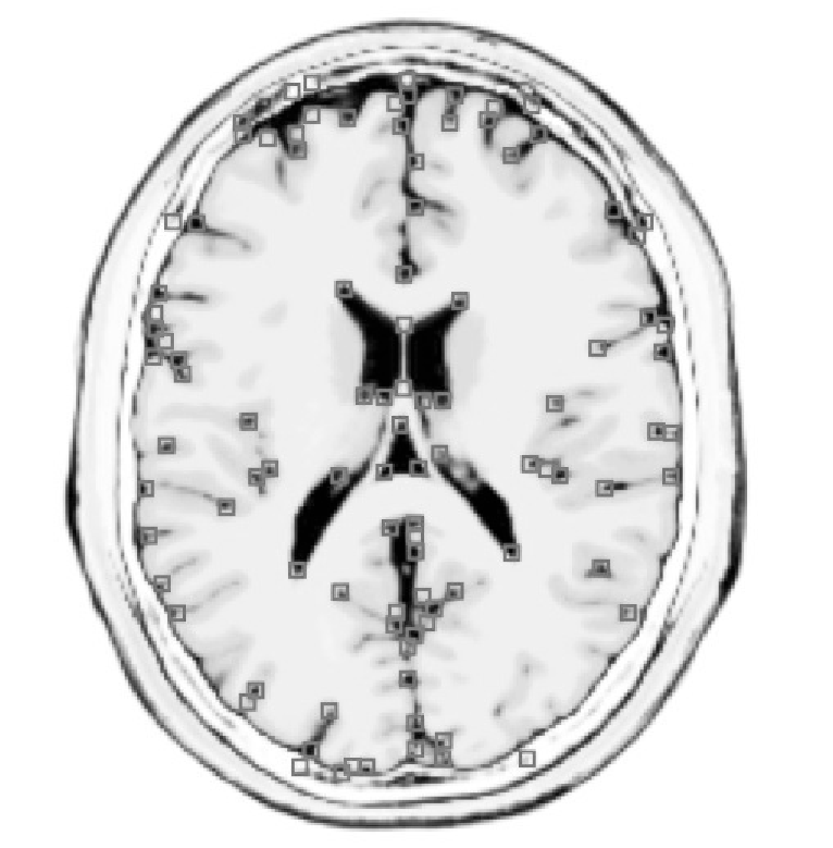
Figure 1: (Left) Corners (gray squares) discovered by the smoothed Harris detector for a brain MRI image. (Right) Schematic representation of the image manifold for the faces shown in polar coordinates ($\alpha,\theta$) where $\alpha$ is the scaling factor and $\theta$ is the rotation angle (Brain image manifold can be represented similarly).

For each image, the number of extracted salient points was set to $N_{c}=100$ maximum, the Gaussian kernel used for saliency detection has a standard deviation $\sigma$ of 2.5% of the graph diameter $d^{*}$. For the value of the connectivity radius $r$ (Sec. 2.2), good results have been obtained if $r=1/15$. With this value, each node in the resulting saliency graphs were connected to an average of 5 other nodes.

Results and discussions:

The ROC curves testing rotation invariance, scaling invariance, and mixed rotation and scaling invariance have been computed for the two databases and for $\mathcal{D}_{\rm ord}$, $\mathcal{D}_{\rm Sp}$ and $\mathcal{D}_{\rm Sp}\mathcal{D}_{\Delta}$. For these two last distances, the ROC curves have been obtained by keeping only the $k=10$ first eigenvalues and GFT coefficients. The ROC curves testing mixed rotation and scaling are shown in Fig. 2 for the two databases. All the related AUCs are summarized in Fig. 3.

For the brain MRI database, $\mathcal{D}_{\rm Sp}$ achieves sensitivities over 90% with false positives rates lower than 10%. Under rotation only, a sensitivity of 95% with a false positives rate of 8% is achieved. Results for the ORL Database of Faces were slightly worse due to the lower number of salient points detected. For all faces, the maximum possible number of salient points, i.e., all the local maxima of the cornerness function, was systematically lower than the imposed maximum of $N_{c}=100$. The hashing was therefore more sensitive to the variations of salient point positions between different transformation of the same image.

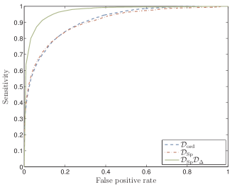
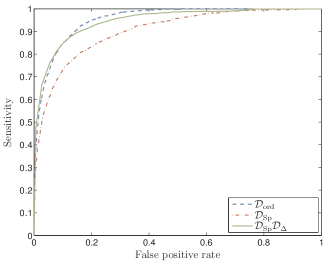
Figure 2: ROC curves for mixed image rotation and scaling: (left) brain database, (right) faces database. The “$-\cdot-$”, dashed and continuous curves show the robustness when $\mathcal{D}_{\rm ord}$, $\mathcal{D}_{\rm Sp}$ and $\mathcal{D}_{\rm Sp}\mathcal{D}_{\Delta}$ are used, respectively.

Database	Transf.	${\mathcal{D}_{\rm ord}}$	${\mathcal{D}_{\rm Sp}}$	${\mathcal{D}_{\rm Sp}\mathcal{D}_{\Delta}}$
	Rotation	0.695	0.926	0.985
Brainweb	Scaling	0.724	0.888	0.967
	Rot. & Scal.	0.787	0.904	0.969
	Rotation	0.892	0.918	0.961
ORL Faces	Scaling	0.933	0.891	0.938
	Rot. & Scal.	0.954	0.902	0.946

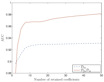
Figure 3: (Left) AUC table for the different transformations of the images using distance between ordered hashing ($\mathcal{D}_{\rm ord}$), distance between spectral hashing ($\mathcal{D}_{\rm Sp}$), and spectral hashing combined with spectra comparison ($\mathcal{D}_{\rm Sp}\mathcal{D}_{\Delta}$). (Right) Area under the ROC curve for increasing number of ISH coefficients and eigenvalues. Most information is contained in the 10 first coefficients after what the AUC remains mostly constant.

For the brain database, an interesting result is that the distance between brain slices that are physically close is shorter than the distance between slices wide apart in the brain. In other words, if we consider the brain MRI as a volumetric image $I_{z}(\boldsymbol{x})=I(x,y,z)$ for which each slice in the database is the result of fixing $z$ to some value, then the expectation of the distance $\mathcal{D}_{\rm Sp}$ between two slices separated along the $z-$axis by a distance $\delta_{z}>0$,

$$m_{d}(\delta_{z})=\mathbb{E}\big{\{}\mathcal{D}_{\rm Sp}(I_{z},I_{z+\delta}):\delta=\pm\delta_{z},z\in\mathbb{R}\big{\}},$$ (3)

is an increasing function of $\delta_{z}$ for $\delta_{z}$ sufficiently close to zero. Fig. 4 shows the evolution of $m_{d}(\delta_{z})$ (with two dashed curves providing the 99% confidence interval on $m_{d}$ estimation) computed over the 100 brain slices rotated and scaled. The expectation of the distance is indeed increasing for $\delta_{z}\leq 10$. This means that the distance $\mathcal{D}_{\rm Sp}$ between ISH truly reflects the difference between visual contents. The MRI was indeed taken with a $z-$resolution of 1mm for which visual contents of contiguous slices are very close, as depicted in Fig. 4. The false positive pairs of images are therefore more likely to be adjacent slides which are visually close than totally different slides.

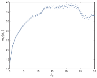
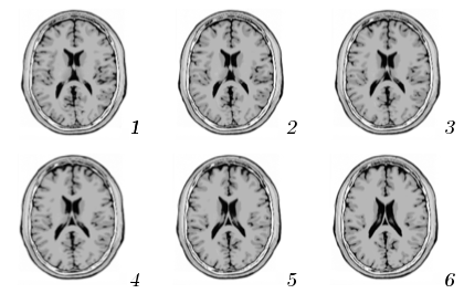
Figure 4: (Left) The expectation of the distance between slices of the brain database is an increasing function of the actual physical distance between slices. (Right) Six contiguous slices of the brain. The visual content does not change much from slice to slice. A suitable image metric should therefore yield low distances between them.

In order to validate the performance of the ISH compared to the naive ordered hashing (OR) ordering the $N_{c}$ values of the saliency function, all the ROC curves were computed using only the $k=10$ first GFT coefficients and the 10 first Laplacian eigenvalues. Therefore, the hash lengths related to the use of $\mathcal{D}_{\rm Sp}$ and $\mathcal{D}_{\rm Sp}\mathcal{D}_{\Delta}$ are both equal to 20, that is, 20% of the tested OR hash length. Results show that the spectral hashing with less coefficients performs as good or better than the naive ordering hashing. It is interesting to quantify the gain in discrimination when the number $k$ of GFT coefficients and eigenvalues increases in the spectral hashing. This can be evaluated by computing the AUC for an increasing number of coefficients. This evolution is depicted in Fig. 3 for both the spectral hashing and the combination of the spectral hashing with the spectral comparison. As a result, the performance does not increase much when more than 2$\times$10 coefficients are retained. The spectral hashing is therefore capable to extract the information useful to discriminate between different visual contents in fewer coefficients.

5 Conclusion

This paper has shown that the geometry of salient point distribution can advantageously be considered in order to form an invariant image hashing. This geometrical inclusion is achieved through the Laplacian spectrum of a Saliency Graph built by connecting geographically close salient points. In consequence, the associated Graph Fourier Transform of some saliency function, that can be improved with the Laplacian eigenvalue distribution, provides a robust and discriminant image hashing. Moreover, compared to the ordered hashing where the knowledge of the salient point distribution is lost, the Invariant Spectral Hashing requires much less values for the same efficiency. In a future research, the impact of the connectivity parameters (like the radius $r$) on the classification procedure will be assessed, together with a careful study of different quantization strategies (e.g., scalar quantization of the different spectra). We expect also to achieve a characterization of images made of several distinct objects arranged on a smooth background. The saliency graph can indeed serve to partition the image thanks to the structure of the first Laplacian eigenvectors (like the zero crossing paths).

References

- [1] F. R. K. Chung. Spectral graph theory. Regional Conference Series in Mathematics, American Mathematical Society, 92:1–212, 1997.
- [2] T. Fawcett. An introduction to ROC analysis. Pattern Recognition Letters, 27(8):861–874, Jun. 2006.
- [3] R. Gal and D. Cohen-Or. Salient geometric features for partial shape matching and similarity. ACM Transactions on Graphics, 25(1):130–150, Jan. 2006.
- [4] C. Harris and M. Stephens. A combined corner and edge detector. In Proceedings of the 4th Alvey Vision Conference, pp. 147–151, 1988.
- [5] E. Kokiopoulou and P. Frossard. Minimum distance between pattern transformation manifolds: Algorithm and applications. IEEE Trans. Pattern Analysis and Machine Intelligence, 31(7):1225–1238, Jul. 2009.
- [6] R. K. S. Kwan, A. C. Evans, and G. B. Pike. MRI simulation-based evaluation of image-processing and classification methods. IEEE Trans. Medical Imaging, 18(11):1085–1097, Nov. 1999.
- [7] Y. Lamdan and H. J. Wolfson. Geometric hashing: A general and efficient model-based recognition scheme. In Proc. Second International Conference on Computer Vision, pp. 238–249, 1988.
- [8] T. Lindeberg. Feature detection with automatic scale selection. International Journal of Computer Vision, 30(2):79–116, 1998.
- [9] M. Mihçak and R. Venkatesan. New iterative geometric methods for robust perceptual image hashing. In ACM CCS Workshop on Security and Privacy in Digital Rights Management, LNCS, 2001.
- [10] V. Monga and B. L. Evans. Perceptual image hashing via feature points: Performance evaluation and tradeoffs. IEEE Trans. Image Processing, 15(11):3452–3465, Nov. 2006.
- [11] F. Samaria and A. Harter. Parameterisation of a stochastic model for human face identification. In IEEE Workshop on Applications of Computer Vision, Sarasota (Florida), Dec. 1994.
- [12] A. Singer. From graph to manifold Laplacian: the convergence rate. Applied and Computational Harmonic Analysis, 21(1):128–134, 2006.
- [13] R. Venkatesan, S.-M. Koon, M. H. Jakubowskil, and P. Moulin. Robust image hashing. In International Conference on Image Processing (ICIP), 2000, 3:664–666, 2000.
- [14] S. Yang. Robust image hash based on cyclic coding the distributed features. In Ninth International Conference on Hybrid Intelligent Systems, pp. 441–444. IEEE Computer Society, 2009.