Zitterbewegung of optical pulses in nonlinear frequency conversion

Abstract

Pulse walk-off in the process of sum frequency generation in a nonlinear $\chi^{(2)}$ crystal is shown to be responsible for pulse jittering which is reminiscent to the Zitterbewegung (trembling motion) of a relativistic freely moving Dirac particle. An analytical expression for the pulse center of mass trajectory is derived in the no-pump-depletion limit, and numerical examples of Zitterbewegung are presented for sum frequency generation in periodically-poled lithium niobate. The proposed quantum-optical analogy indicates that frequency conversion in nonlinear optics could provide an experimentally accessible simulator of the Dirac equation.

1 Introduction

Originally predicted by Schrödinger in the study of the Dirac equation [1], Zitterbewegung (ZB) refers to the trembling motion of a freely-moving relativistic quantum particle that arises from the interference between the positive- and negative-energy parts of the spinor wave function [2]. For a free electron, the Dirac equation predicts the ZB to have an extremely small amplitude (of the order of the Compton wavelength $\simeq 10^{-12}\;{\rm m}$) and an extremely high frequency ($\simeq 10^{21}\;{\rm Hz}$), making such an effect experimentally inaccessible. In addition, the physical relevance of ZB in relativistic quantum mechanics is a controversial issue because such an effect arises in the framework of the single-particle picture of the Dirac equation, but not in quantum field theory [3, 4]. The notion of ZB and resulting formalism, however, are not peculiar to relativistic quantum dynamics, and phenomena analogous to ZB, which underly the same mathematical model of the Dirac equation, have so far predicted in a wide variety of quantum and even classical physical systems, including among others semiconductors and quantum wells [5, 6, 7], trapped ions [8], graphene [9, 10, 11, 12], cold atoms [13, 14], acoustic [15] and photonic [16, 17, 18] systems. Simulations of relativistic quantum effects using experimentally-accessible physical set-ups, in which parameter tunability allows access to different physical regimes, have seen in recent years an increasing interest, culminating to the very recent first experimental observation of a quantum analogue of ZB using a single trapped ion set to behave as a free relativistic quantum particle [19]. In the optical context, the use of photonic systems to mimic quantum phenomena in the lab has seen a continuous and increasing interest (see, for instance, [20] and references therein); in particular, optical analogues of the relativistic ZB have been recently proposed to occur in photonic crystals [16], metamaterial slabs [17], and binary waveguide arrays [18]. In this work it is shown theoretically that a classical analogue of ZB can be observed in a much simpler and well-known set-up of nonlinear optics, namely in the process of sum frequency generation of light waves in a nonlinear $\chi^{(2)}$ medium [21] in presence of pulse (or spatial) walk off. In the nonlinear optics context, optical three-wave interaction (TWI) in nonlinear $\chi^{(2)}$ media in presence of temporal (or spatial) walk-off is a well-known process, which has been widely investigated especially in connection to pulse compression of ultrashort pulses and to TWI soliton theory (see, for instance, [22, 23, 24, 25, 26, 27]). Notably, the nonlinear TWI equations are solvable by inverse scattering methods [22]. However, the ZB phenomenon discussed in this work and the idea of exploiting nonlinear optics to mimic the Dirac equation have not been addressed in such previous studies.

2 Basic model and quantum-optical analogy

The starting point of our analysis is provided by a standard model of TWI in a nonlinear quadratic medium describing propagation of either optical pulses or optical beams at frequencies $\omega_{1}$, $\omega_{2}$ and $\omega_{3}=\omega_{1}+\omega_{2}$ in presence of either group velocity mismatch or spatial walk-off. For the sake of definiteness, we will consider here the case of optical pulse interaction in presence of temporal walk-off (i.e. of group velocity mismatch), however the results hold also for spatial beam propagation in a quadratic medium with spatial walk-off provided that the temporal coordinate is replaced by a transverse spatial coordinate (see, for instance, [27]). Assuming that group velocity dispersion is negligible, in the plane-wave approximation and assuming perfect phase matching, pulse propagation in the $\chi^{(2)}$ medium is described by the following set of nonlinear coupled equations [21, 22, 23, 24, 25, 28]:

$$\left(\frac{\partial}{\partial z}+\frac{1}{v_{g1}}\frac{\partial}{\partial t}\right)A_{1} = i\rho A_{2}^{*}A_{3}$$ (1)

$$\left(\frac{\partial}{\partial z}+\frac{1}{v_{g2}}\frac{\partial}{\partial t}\right)A_{2} = i\rho A_{1}^{*}A_{3}$$ (2)

$$\left(\frac{\partial}{\partial z}+\frac{1}{v_{g3}}\frac{\partial}{\partial t}\right)A_{3} = i\rho^{*}A_{1}A_{2}$$ (3)

where $A_{l}=A_{l}(z,t)$ ($l=1,2,3$) is the amplitude of the electric field envelope at the carrier frequencies $\omega_{l}$, normalized such that $|A_{l}|^{2}$ is the photon flux at frequency $\omega_{l}$, $v_{gl}$ is the group velocity in the medium at frequency $\omega_{l}$, and $\rho$ is the strength of the nonlinear interaction, which reads explicitly

$$\rho=\frac{d_{eff}}{c_{0}}\sqrt{\frac{2\hbar\omega_{1}\omega_{2}\omega_{3}}{\epsilon_{0}c_{0}n_{1}n_{2}n_{3}}},$$ (4)

where $n_{l}$ is the refractive index of the medium at frequency $\omega_{l}$ ($l=1,2,3)$, $c_{0}$ is the speed of light in vacuum, and $d_{eff}=(1/2)\chi^{(2)}_{eff}$ is the effective nonlinear coefficient. To achieve perfect phase matching, a quasi-phase-matching (QPM) grating for the nonlinear susceptibility $\chi^{(2)}$ can be employed; in this case one has (see, for instance, [28])

$$d_{eff}=\frac{1}{2}\overline{\chi^{(2)}(z)\exp(i\Delta kz)}$$ (5)

where $\Delta k=(\omega_{3}n_{3}-\omega_{2}n_{2}-\omega_{1}n_{1})/c_{0}$ is the phase mismatch of the three waves and the overbar denotes a spatial average over a few modulation periods of the QPM grating. Equations (1-3) admit of the following two invariants along the propagation distance $z$

$$\mathcal{I}_{1,2}=\int_{-\infty}^{\infty}dt(|A_{1,2}|^{2}+|A_{3}|^{3})$$ (6)

which correspond to photon flux conservation (Manley-Rowe invariants) in the frequency conversion process. Solitary waves of Eqs.(1-3) in the fully nonlinear regime, including trapped bright-dark-bright solitary waves with locked velocity, have been investigated in Refs.[22, 23, 24, 25, 26, 27]. To study the analogue of ZB in the frequency conversion process, we assume here that at the input plane $z=0$ the nonlinear crystal is excited by a strong and nearly continuous-wave pump field at frequency $\omega_{1}$, and by a weak and short signal pulse at frequency $\omega_{2}$ and temporal profile $g(t)$. Under such assumptions, the invariance of $\mathcal{I}_{1,2}$ implies that the pump wave remains nearly undepleted along the propagation distance, and Eqs.(1-3) reduce to the following two linear coupled-field equations describing sum-frequency generation in the undepleted regime

$$\left(\frac{\partial}{\partial z}+\frac{1}{v_{g2}}\frac{\partial}{\partial t}\right)A_{2} = -i\kappa A_{3}$$ (7)

$$\left(\frac{\partial}{\partial z}+\frac{1}{v_{g3}}\frac{\partial}{\partial t}\right)A_{3} = -i\kappa A_{2}$$ (8)

where we have set $\kappa\equiv-\rho A_{1}^{*}=\rho{\sqrt{I_{1}/\hbar\omega_{1}}}$ and $I_{1}$ is the intensity of the pump field. Without loss of generality, $\kappa$ can be assumed to be real-valued and positive. Note that, in the absence of group velocity mismatch for the signal and second-harmonic waves at frequencies $\omega_{2}$ and $\omega_{3}$, i.e. for $v_{g2}=v_{g3}$, the solution to Eqs.(7) and (8) is analogous to the one for stationary fields [21], which shows a well-known oscillatory power transfer, along the propagation distance $z$, between the two fields with spatial period $\pi/\kappa$; namely one has

$$A_{2}(z,t) = g\left(t-\frac{z}{v_{g}}\right)\cos(\kappa z)$$ (9)

$$A_{3}(z,t) = -ig\left(t-\frac{z}{v_{g}}\right)\sin(\kappa z)$$ (10)

where $v_{g}=v_{g2}=v_{g3}$. Note that, in spite of the oscillatory power transfer in the frequency conversion process, the two pulses propagates with the common group velocity $v_{g}$ and do not show any trembling (jitter) motion. If the group velocity mismatch is not negligible ($v_{g2}\neq v_{g3}$), the solution to Eqs.(7) and (8) is more involved, and is given by Eqs.(25) and (26) discussed in the next section. Here we anticipate that, in this regime, the oscillatory power transfer between the two fields is generally accompanied by an oscillatory motion of the pulse center of mass, which is reminiscent of ZB for the free relativistic Dirac electron. To highlight such an analogy in a formal way, it is worth introducing the coordinates of a moving frame

$$\xi=z\;,\;\;\eta=t-z/v_{g}$$ (11)

where the velocity $v_{g}$ is defined by the relation

$$\frac{1}{v_{g}}=\frac{1}{2}\left(\frac{1}{v_{g2}}+\frac{1}{v_{g3}}\right).$$ (12)

In the moving frame, Eqs.(7) and (8) take the form

$$\left(\frac{\partial}{\partial\xi}+\delta\frac{\partial}{\partial\eta}\right)A_{2} = -i\kappa A_{3}$$ (13)

$$\left(\frac{\partial}{\partial\xi}-\delta\frac{\partial}{\partial\eta}\right)A_{3} = -i\kappa A_{2}$$ (14)

where we have set

$$\delta=\frac{1}{2}\left(\frac{1}{v_{g2}}-\frac{1}{v_{g3}}\right).$$ (15)

Equations (13) and (14) are supplemented with the boundary conditions

$$A_{2}(0,\eta)=g(\eta)\;,\;A_{3}(0,\eta)=0.$$ (16)

After introduction of the spinor wave field $\psi=(A_{2},A_{3})^{T}$, Eqs.(13) and (14) can be finally cast into the Dirac form

$$i\frac{\partial\psi}{\partial\xi}=-i\sigma_{z}\delta\frac{\partial\psi}{\partial\eta}+\kappa\sigma_{x}\psi$$ (17)

where $\sigma_{x}$ and $\sigma_{z}$ are the Pauli matrices. Note that, after the formal change

$$\delta \rightarrow c$$

$$\kappa \rightarrow \frac{mc^{2}}{\hbar}$$ (18)

$$\xi \rightarrow t\;,\;\eta\rightarrow x$$

Eq.(17) corresponds to the one-dimensional Dirac equation for a relativistic particle of mass $m$ in absence of external fields, moving alon the $x$ axis, written in the Weyl representation [2]. Therefore, the temporal evolution of the spinor wave function $\psi$ for the Dirac particle is mapped into the spatial evolution of the envelopes $A_{2}$ and $A_{3}$ for signal and sum-frequency pulses, respectively, whereas the spatial coordinate of the Dirac particle is mapped into the retarded time $\eta$ of the optical pulses.

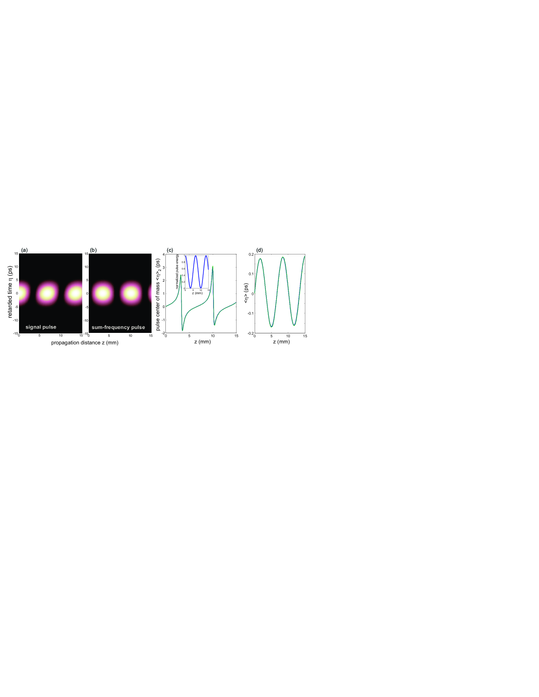
Figure 1: (color online) Sum frequency generation in a $L=1.5$-cm-long PPLN crystal showing ZB of the signal pulse. (a) and (b): snapshots of the intensity distributions of signal [Fig.1(a)] and sum-frequency [Fig.1(b)] pulses versus propagation distance $z$. (c) Numerically-computed behavior of pulse center of mass $\langle\eta\rangle_{2}$ for the signal field versus propagation distance (solid curve), and corresponding behavior predicted by Eq.(28) (dotted curve, almost overlapped with the solid one). The inset depicts the behavior of the normalized photon fluence $\phi_{2}(z)/\phi_{2}(0)$ of signal field versus propagation distance, showing the oscillatory exchange of power between the signal and sum-frequency waves. (d) Numerically-computed behavior of $\langle\eta\rangle$, defined by Eq.(19), versus propagation distance (solid curve), and corresponding behavior predicted by Eq.(29) (dotted curve, almost overlapped with the solid one). The input pulse duration is $\tau_{p}=5$ ps. Other parameter values are given in the text.

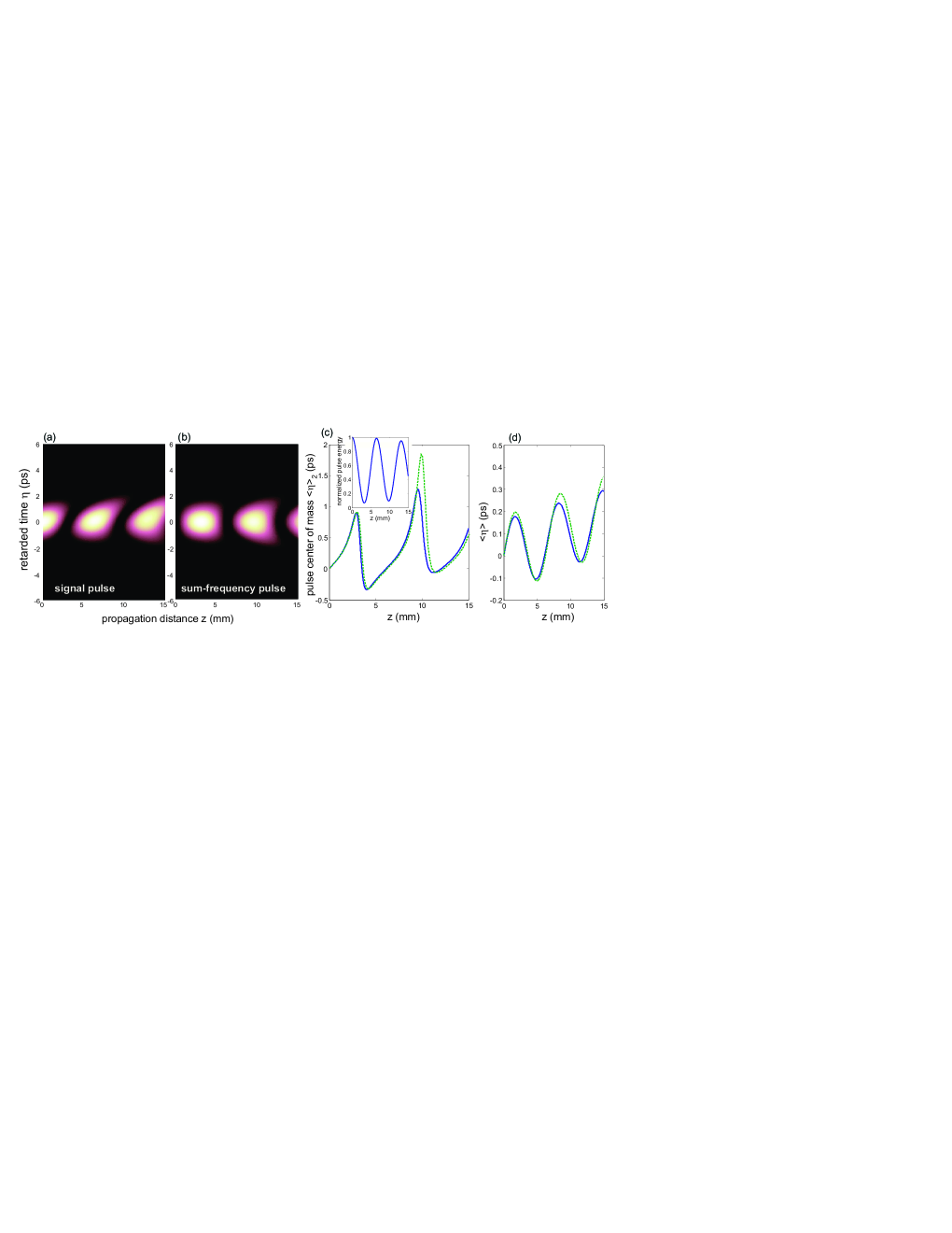
Figure 2: (color online) Same as Fig.1, but for an input pulse duration $\tau_{p}=1.5$ ps.

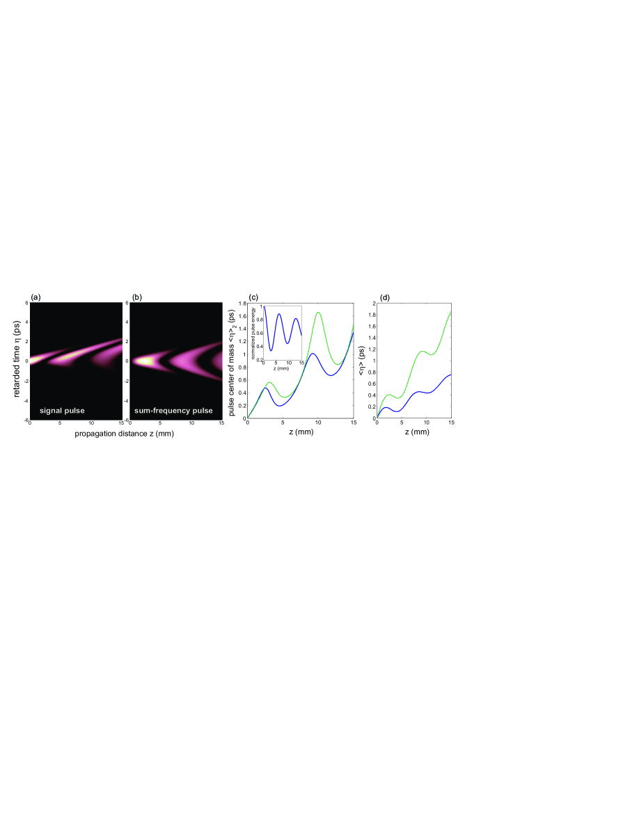
Figure 3: (color online) Same as Fig.1, but for an input pulse duration $\tau_{p}=0.5$ ps.

3 Zitterbewegung of optical pulses

For the Dirac equation (17), ZB refers to the rapid oscillatory motion of the expectation value of the particle position

$$\langle\eta\rangle(\xi)\equiv\frac{\int_{-\infty}^{\infty}d\eta\;\eta\left(|A_{2}|^{2}+|A_{3}|^{2}\right)}{\int_{-\infty}^{\infty}d\eta\left(|A_{2}|^{2}+|A_{3}|^{2}\right)}$$ (19)

around its mean trajectory, which arises whenever negative- and positive-energy eigenstates of the Dirac equation are simultaneously excitated by the initial condition. Note that, indicating by $\langle\eta\rangle_{2}(\xi)$ and $\langle\eta\rangle_{3}(\xi)$ the (temporal) center of mass of the signal and sum-frequency pulses at the crystal plane $\xi=z$, i.e.

$$\langle\eta\rangle_{2,3}(\xi)\equiv\frac{\int_{-\infty}^{\infty}d\eta\;\eta|A_{2,3}(\xi,\eta)|^{2}}{\int_{-\infty}^{\infty}d\eta|A_{2,3}(\xi,\eta)|^{2}}$$ (20)

one can write

$$\langle\eta\rangle(\xi)=\frac{\phi_{2}(\xi)\langle\eta\rangle_{2}(\xi)+\phi_{3}(\xi)\langle\eta\rangle_{3}(\xi)}{\mathcal{I}_{2}}$$ (21)

where $\phi_{2,3}(\xi)=\int d\eta|A_{2,3}(\xi,\eta)|^{2}$ are the photon fluences of the signal and sum-frequency pulses at the plane $z=\xi$, respectively, and $\mathcal{I}_{2}=\phi_{2}(\xi)+\phi_{3}(\xi)=\phi_{2}(0)$ is the Manley-Rowe invariant. In particular, if the initial pulse envelope $g(t)$ is symmetric, i.e. $g(-t)=g(t)$, as it will be shown below one has $\langle\eta\rangle_{3}(\xi)=0$, and thus according to Eq.(21) the ZB of the Dirac particle for Eq.(17) can be simply retrieved from the temporal jitter $\langle\eta\rangle_{2}(\xi)$ and fractional energy $\phi_{2}(\xi)/\phi_{2}(0)$ of the signal pulse.
The solution to Eqs.(13) and (14) with $\delta\neq 0$ and with the boundary conditions (16) can be readily obtained in the spectral (Fourier) domain. Indicating by $\hat{A}_{2,3}(\xi,\omega)=(1/2\pi)\int d\eta A_{2,3}(\xi,\eta)\exp(-i\eta\omega)$ the spectra of the signal and sum-frequency fields at the propagation plane $\xi$, one has

$$\hat{A}_{2}(\xi,\omega) = \hat{g}(\omega)\left[\cos(\beta\xi)-i\frac{\omega\delta}{\beta}\sin(\beta\xi)\right]$$ (22)

$$\hat{A}_{3}(\xi,\omega) = -\frac{i\kappa}{\beta}\hat{g}(\omega)\sin(\beta\xi)$$ (23)

where $\hat{g}(\omega)=(1/2\pi)\int d\eta g(\eta)\exp(-i\eta\omega)$ is the spectrum of the signal pulse incident onto the crystal at $\xi=0$, and

$$\beta(\omega)=\sqrt{\kappa^{2}+\omega^{2}\delta^{2}}.$$ (24)

In the temporal domain, the inverse Fourier transform of Eqs.(22) and (23) yields the following exact solution for the sum-frequency and signal pulses traveling along the crystal

$$A_{3}(\xi,\eta)=-\frac{i\kappa}{2\delta}\int_{-\delta\xi}^{\delta\xi}d\theta g(\theta+\eta)J_{0}\left(\kappa\sqrt{\xi^{2}-\frac{\theta^{2}}{\delta^{2}}}\right)$$ (25)

$$A_{2}(\xi,\eta) = \frac{g(\eta+\delta\xi)+g(\eta-\delta\xi)}{2}$$ (26)

$$+ \frac{1}{2\delta}\int_{-\delta\xi}^{\delta\xi}d\theta g(\theta+\eta)\frac{\partial}{\partial\xi}J_{0}\left(\kappa\sqrt{\xi^{2}-\frac{\theta^{2}}{\delta^{2}}}\right)$$

$$- \frac{1}{2}\int_{-\delta\xi}^{\delta\xi}d\theta\frac{\partial g}{\partial\eta}(\theta+\eta)J_{0}\left(\kappa\sqrt{\xi^{2}-\frac{\theta^{2}}{\delta^{2}}}\right)$$

where $J_{0}$ is the zero-order Bessel function of first kind. To calculate $\langle\eta\rangle$, $\langle\eta\rangle_{2}$ and $\langle\eta\rangle_{3}$, let us assume, for the sake of simplicity, that the signal pulse envelope $g(t)$ at the input crystal plane has a symmetric profile (with e.g. a Gaussian or a sech shape) satisfying the condition $g(-\eta)=g(\eta)$. In this case, from Eq.(25) it follows that $A_{3}(\xi,-\eta)=A_{3}(\xi,\eta)$, and thus

$$\langle\eta\rangle_{3}(\xi)=0\;,\;\;\langle\eta\rangle(\xi)=\frac{\phi_{2}(\xi)}{\phi_{2}(0)}\langle\eta\rangle_{2}(\xi).$$ (27)

The explicit expression of $\langle\eta\rangle_{2}(\xi)$, as obtained by substitution of Eq.(26) into Eq.(20), turns out to be rather cumbersome and not of easy physical interpretation. However, for a signal spectrum $\hat{g}(\omega)$ narrow at around $\omega=0$ with a spectral width $\Delta\omega$ much smaller than $\kappa/\delta$, i.e. for a relatively long input pulse, simple approximate expressions for $\langle\eta\rangle_{2}(\xi)$ and $\langle\eta\rangle(\xi)$ can be obtained, which read explicitly

$$\langle\eta\rangle_{2}(\xi) \simeq \xi\frac{\delta^{3}}{\kappa^{2}}\frac{\Delta\omega^{2}}{\cos^{2}(\kappa\xi)+\frac{\delta^{2}\Delta\omega^{2}}{\kappa^{2}}}$$ (28)

$$+ \frac{\delta}{2\kappa}\frac{\sin(2\kappa\xi)}{\cos^{2}(\kappa\xi)+\frac{\delta^{2}\Delta\omega^{2}}{\kappa^{2}}}$$

$$\langle\eta\rangle(\xi) \simeq \xi\frac{\delta^{3}\Delta\omega^{2}}{\kappa^{2}}+\frac{\delta}{2\kappa}\sin(2\kappa\xi)$$ (29)

where $\Delta\omega$ is the spectral width of the input signal pulse, defined by

$$\Delta\omega^{2}=\frac{\int d\omega\omega^{2}|\hat{g}(\omega)|^{2}}{\int d\omega|\hat{g}(\omega)|^{2}}.$$ (30)

Equation (29) corresponds to the well-known approximate expression of ZB in relativistic quantum mechanics (see, for instance, [2, 19]), whereas Eq.(28) shows the signature of ZB in the oscillatory motion of the signal pulse center of mass as it propagates along the crystal. Note that such an oscillatory motion, that arises from the second term on the right hand side of Eq.(29), is superimposed to a slight drift term [the first term on the right hand side of Eq.(29)]. The oscillatory motion of $\langle\eta\rangle$ and $\langle\eta\rangle_{2}$ along the propagation coordinate $\xi$ of the crystal basically follows the oscillatory-like of optical transfer between signal and sum-frequency pulses. Note also that, according to Eq.(28) and because of the assumption $\delta\Delta\omega/\kappa\ll 1$, the pulse center of mass $\langle\eta\rangle_{2}(\xi$ takes large values at the propagation distances $\xi=\pi/2\kappa$, $\xi=\pi/\kappa$, $\xi=3\pi/2\kappa$, … where most of the signal field is converted into the sum-frequency field.
As an example, let us consider the process of sum frequency generation in a nonlinear periodically-poled lithium-niobate (PPLNB) crystal (see, for instance, [29]) assuming $\lambda_{1}=1550$ nm, $\lambda_{2}=810$ nm, and $\lambda_{3}=532$ nm for the wavelengths (in vacuum) of pump, signal and sum-frequency waves, respectively. From Sellmeir equations [30], one can estimate at 25^oC and for extraordinary waves $n_{1}=2.1381$, $n_{2}=2.1748$, $n_{3}=2.2343$, $v_{g2}/c_{0}=0.4422$, $v_{g3}/c_{0}=0.4069$ and a QPM period of $\Lambda=2\pi/\Delta k\simeq 7.39\;\mu$m, which is easily accessible with current poling technology. For first-order QPM with alternating sign +/- of $\chi^{(2)}$ with period $\Lambda/2$, the effective nonlinear coefficient is given by [29] $d_{eff}=(2/\pi)d$, where $d$ is the element of the nonlinear $d$-tensor of the crystal involved in the parametric interaction ($d=d_{33}\simeq 27\;{\rm pm/V}$ for extraordinary waves). As an input signal pulse, we assume a Gaussian profile $g(t)\propto\exp(-t^{2}/\tau_{0}^{2})$ with a full-width at half maximum (FWHM) pulse duration $\tau_{p}=(\sqrt{2{\rm log}2})\tau_{0}$ and spectral pulse width $\Delta\omega=1/\tau_{0}$. As an example, Figs.1(a) and 1(b) show the evolution of the pulse intensity profiles $|A_{2}(\xi,\eta)|^{2}$ and $|A_{3}(\xi,\eta)|^{2}$ of signal and sum-frequency fields, respectively, in a $L=$1.5-cm-long PPLN crystal as obtained by direct numerical analysis of Eqs.(1-3), for a signal pulse duration $\tau_{p}=5$ ps of low peak intensity ($1$ W/cm²) and an intensity of the continuous-wave pump field $I_{1}=\hbar\omega_{1}|A_{1}|^{2}$ of $1\;{\rm MW/cm^{2}}$, corresponding to $\kappa\simeq 0.4656\;{\rm mm}^{-1}$ and $\delta\Delta\omega/\kappa\simeq 0.0827$. The numerical results of Fig.1 are with excellent accuracy reproduced by the analytical solutions (25) and (26), derived in the no-pump depletion limit. Figures 1(c) and 1(d) show the corresponding behavior, along the crystal coordinate $\xi=z$, of the normalized photon fluence $\phi_{2}(\xi)/\phi_{2}(0)$ [inset of Fig.1(c)], pulse center of mass $\langle\eta\rangle_{2}(\xi)$ of signal field [solid curve in Fig.1(c)], and ZB amplitude $\langle\eta\rangle(\xi)=[\phi_{2}(\xi)/\phi_{2}(0)]\langle\eta\rangle_{2}(\xi)$ [solid curve in Fig.1(d)]. In Figs.1(c) and (d), the behaviors of $\langle\eta\rangle_{2}(\xi)$ and $\langle\eta\rangle(\xi)$, as predicted by Eqs.(28) and (29), are also shown (dotted curves, almost overlapped with the solid ones). Note that, according to the theoretical analysis, the center of mass of the signal pulse undergoes a clear oscillatory motion, superimposed to a slight drift [arising from the first term on the right hand side of Eq.(28)]. For spectrally broader signal pulses, ZB can not be accurately described by the simple Eqs.(28) and (29), however the oscillatory motion of the pulse center of mass, superimposed to a drift motion, is still observed in numerical simulations. This is shown, as an example, in Figs.2 and 3, where pulse duration of the injected signal pulse has been reduced to $\tau_{p}=1.5$ ps in Fig.2 (corresponding to $\delta\Delta\omega/\kappa\simeq 0.2758$), and to $\tau_{p}=0.5$ ps in Fig.3 (corresponding to $\delta\Delta\omega/\kappa\simeq 0.827$). In an experiment, a measurement of the pulse center of mass at internal planes of the nonlinear crystal could be a nontrivial task, whereas autocorrelation measurements can readily reveal a jitter of the output pulse, at the exit of the crystal, with respect to a reference case. Owing to the dependence of the sinusoidal terms entering in Eq.(28) on the product $\kappa\xi\propto\sqrt{I_{1}}\xi$, in an experiment the signature of ZB can be easier revealed by monitoring the center of mass of the signal pulse at the output plane $\xi=L$ of the crystal as a function of the pump intensity $I_{1}$. This is shown, as an example, in Fig.4, where the numerically-computed behavior of $\langle\eta\rangle_{2}$ at the output crystal plane versus the intensity $I_{1}$ of the pump field is depicted, together with the approximate prediction based on Eq.(28).

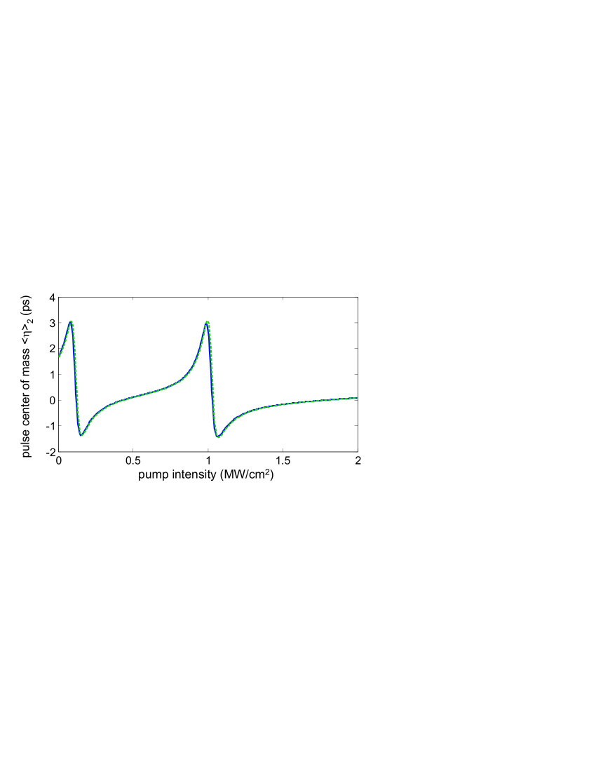
Figure 4: (color online) Numerically-computed behavior of the center of mass $\langle\eta\rangle_{2}$ for the signal pulse at the output of the PPLN crystal versus the intensity $I_{1}$ of the pump field. The crystal length is $L=1$ cm, the input pulse duration of the signal field is $\tau_{p}=5$ ps. The dotted curve in the figure is the behavior of $\langle\eta\rangle_{2}$ predicted by Eq.(28).

4 Conclusions

In this work, a photonic analogue of the trembling motion (Zitterbewegung) of a free relativistic Dirac particle, based on frequency conversion of short optical pulses in a nonlinear quadratic medium, has been presented. The analogy, which stems from the mathematical similarity between the Dirac equation of a massive particle and the coupled equations describing sum frequency generation in the presence of pulse walk-off, indicates that well-known and experimentally accessible nonlinear optical processes could be exploited to simulate the Dirac equation in an optical setting. As compared to other classical and quantum analogues of Zitterbewegung recently proposed in the literature, based on trapped ions [8, 19], graphene [9, ZB4_1, 11, 12] or photonic crystals, superlattices or metamaterials [16, 17, 18], our proposal may show a simpler experimental access and could stimulate further search for nonlinear optics analogues of relativistic quantum phenomena. For example, engineering of the QPM grating could be exploited to introduce in Eq.(17) a $\xi$-dependence of $\kappa$, i.e. to simulate the dynamics of a relativistic Dirac particle with a time-varying mass [31]. Likewise, if the temporal dependence of the pump pulse is included in the analysis and assuming $v_{g1}=v_{g}$, an $\eta$-dependence of the mass $\kappa$ is introduced in Eq.(17), which enables to mimic a relativistic Dirac particle in a Lorentz scalar potential [2].

The author acknowledges financial support by the Italian MIUR (Grant No. PRIN-2008-YCAAK project ”Analogie ottico-quantistiche in strutture fotoniche a guida d’onda”).

References

- [1] Schrödinger E 1930 Sitz. Preuss. Akad. Wiss. Phys.-Math. Kl. 24 418
- [2] W. Greiner 1990 Relativistic Quantum Mechanics (Berlin: Springer- Verlag)
- [3] Barut A O and Bracken A J 1981 Phys. Rev. D 23 2454
- [4] Krekora P, Su Q and Grobe R 2004 Phys. Rev. Lett. 93 043004
- [5] Ferrari L and Russo G 1990 Phys. Rev. B 42 7454 (1990)
- [6] Schliemann J, Loss D and Westervelt R M 2005 Phys. Rev. Lett. 94 206801
- [7] Zawadzki W 2005 Phys. Rev. B 72 085217
- [8] Lamata L, León J, Schätz T and Solano E 2007 Phys. Rev. Lett. 98 253005
- [9] Cserti J and David G 2006 Phys. Rev. B 74 172305
- [10] Rusin T M and Zawadzki W 2007 Phys. Rev. B 76 195439
- [11] Maksimova G M, Demikhovskii V Ya and Frolova E V 2008 Phys. Rev. B 78 235321
- [12] Rusin T M and Zawadzki W 2009 Phys. Rev. B 80 045416
- [13] Vaishnav J Y and Clark C W 2008 Phys. Rev. Lett. 100 153002
- [14] Zhang Q, Gong J and Oh C H 2010 Phys. Rev. A 81 023608
- [15] Zhang X and Liu Z 2008 Phys. Rev. Lett. 101 264303
- [16] Zhang X 2008 Phys. Rev. Lett. 100 113903
- [17] Wang L G, Wang Z G and Zhu S Y 2009 EuroPhys. Lett. 86 47008
- [18] Longhi S 2010 Opt. Lett. 35 235
- [19] Gerritsma R, Kirchmair G, Zähringer F, Solano E, Blatt R and Roos C F 2010 Nature 463 68
- [20] Longhi S 2009 Laser Photon. Rev. 3 243
- [21] R. W. Boyd 2003 Nonlinear Optics (New York: Academic Press).
- [22] Kaup D J, Reiman A and Bers A 1979 Rev. Mod. Phys. 51 275
- [23] Ibragimov E and Struthers A 1997 J. Opt. Soc. Am. B 14 1472
- [24] Ibragimov E, Struthers A and Kaup D J 1998 Opt. Comm. 152 101
- [25] Ibragimov E, Struthers A A , Kaup D J, Khaydarov J D and Singer K D 1999 Phys. Rev. E 59 6122
- [26] Degasperis A, Conforti M, Baronio F and Wabnitz S 2006 Phys. Rev. Lett. 97 093901
- [27] Baronio F, Conforti M, De Angelis C, Degasperis A, Andreana M, Couderc V and Barthélémy A 2010 Phys. Rev. Lett. 104 113902
- [28] Longhi S, Marano M and Laporta P 2002 Phys. Rev. A 66 033803
- [29] Roussev R V, Langrock C, Kurz J R and Fejer M M 2004 Opt. Lett. 29 1518
- [30] Edwards G J and Lawrence M 1984 Opt. Quantum Electron. 16 373
- [31] See, for instance: Maamache M and Lakehal H 2004 EuroPhys. Lett. 67, 695