High precision spectra at large redshift for dynamical DE cosmologies

Abstract

The next generation mass probes will investigate DE nature by measuring non–linear power spectra at various $z$, and comparing them with high precision simulations. Producing a complete set of them, taking into account baryon physics and for any DE state equation $w(z)$, would really be numerically expensive. Regularities reducing such duty are essential. This paper presents further n–body tests of a relation we found, linking models with DE state parameter $w(z)$ to const.–$w$ models, and also tests the relation in hydro simulations.

1 Introduction

The background metrics of space–time can be written in the forms

$~{}~{}~{}~{}~{}~{}~{}~{}~{}~{}~{}~{}~{}~{}~{}~{}~{}~{}~{}~{}~{}~{}~{}~{}~{}~{}~{}~{}~{}~{}~{}ds^{2}=c^{2}dt^{2}-a^{2}(t)\,d\ell^{2}=a^{2}(\tau)\,(d\tau^{2}-d\ell^{2})$

defining ordinary or conformal time, $t$ or $\tau$. In systems which abandoned cosmic expansion, the former expression yields the Minkowskian metrics: the no longer growing scale factor can be inglobated in spatial coordinates. In such systems $t$ is the natural time coordinate; e.g., many cyclic motions become (quasi–)periodical in respect to $t$. On the contrary, when a system resent the overall expansion, the natural time coordinate is $\tau$. For instance, sonic waves in the pre–recombination plasma, are (quasi–)periodical in respect to $\tau$. This periodicity yields the setting of maxima and minima in CMB spectra, as well as the scales of BAO’s in matter spectra.

Let us consider then the comoving distance between today’s observer and the LSB (last scattering band), $L=\int_{rec}^{0}d\ell$. It coincides with the conformal time $T=\int_{rec}^{0}d\tau$ a photon takes to reach the observer from the LSB. Accordingly, if two models have the same comoving distance from the LSB, we expect them to share those features which are determined by the cosmological dynamics. As a matter of fact, it has been known since several years [1] that, if they share $\Omega_{c,b}$, $h$ and $n_{s}$ (density parameters, Hubble parameter in units of 100 (km/s)/Mpc, primeval scalar index), their linear spectra are quite close. In particular, models with the same conformal age, differing just because of DE state equation, exhibit almost coincident linear spectra.

When non–linear effects are taken into account, the dynamics is no longer simply ruled by $\tau$. Non linear spectral deformations arise when matter halos form, abandoning the overall expansion. The point is whether they are so widely spread to yield a significantly discrepant spectral behavior at a given $k$–scale. Greater $k$’s correspond to scales entering a non–linear regime earlier; therefore, we expect greater discrepancies at greater $k$’s.

A test of these expectations can only be performed in a numerical way, by running model simulations. Let us then outline that forthcoming tomographic lensing experiments (see, e.g., [2]) will be able to measure spectra with a precision $\cal O$$(1\,\%)$ [3], so that this is the limit above which spectral discrepancies can no longer be disregarded. In turn, such experiments are expected to test spectra up to $k\simeq 10\,h$Mpc^-1, corresponding to length scales $\cal O$$(0.5\,h^{-1}$Mpc$)$, well inside galaxy clusters. To test spectral regularities, then, hydro effects cannot be disregarded.

A number of authors have considered these problems in some detail. The $k$ value above which hydrodynamics causes spectral distorsions $>1\,\%$ has been found to be $\sim 2$–$3\,h\,$Mpc^-1 [4]. Models with an assigned polynomial DE state equation $w(z)$ (models $\cal A$) were then compared with models with constant $w$ (models $\cal W$, or auxiliary models), selected so to have the same $L$ and the same $\sigma_{8}$ (mean square density fluctuation at 8$\,h^{-1}$Mpc), besides of $\Omega_{b,c}$ and $h$ [5]. Spectral discrepancies, within $k\sim 2$–$3\,h\,$Mpc^-1 were found to keep within $1\,\%$.

A critical feature of forthcoming mass probes is their capacity to explore the Universe at $z>0$. Models with the same conformal age at $z=0$, and different DE state equation, have different ages at $z>0$ and spectral discrepancies soon exceed $1\,\%$. In principle, then, one should find an auxiliary model $\cal W$$(z)$ of $\cal A$, at any $z$. But equal $H$ at $z\neq 0$ means different $H$ at $z=0$. Accordingly, simulations performed in boxes of identical size in units of $h_{o}^{-1}$Mpc, can no longer be compared (the _o suffix is used just here, to outline that $h$ is taken at $z=0$). If boxes of suitable different sizes are then used, sample variance is the dominant effect.

This difficulty was overcome by abandoning the request that $\cal A$ and $W(z)$ have the same $H(z)$, and requiring them to share just the reduced density parameters $\omega_{c,b}=\Omega_{c,b}h^{2}$ (weak requirement) [7]. The definition of $\rho_{cr}$ (critical density) however implies that, at any $z$,

$~{}~{}~{}~{}~{}~{}~{}~{}~{}~{}~{}~{}~{}~{}~{}~{}~{}~{}~{}~{}~{}~{}~{}~{}~{}~{}~{}~{}~{}~{}~{}~{}~{}~{}~{}\Omega_{c,b}\times H^{2}=\Omega_{c,b}\times(8\pi G/3)\rho_{cr}~{},$

so that the $\omega_{c,b}\propto\Omega_{c,b}H^{2}$ scales as $\Omega_{c,b}\rho_{cr}=\rho_{c,b}\propto a^{-3}$, indipendently of DE nature. Models with equal $\omega_{c,b}$ at $z=0$ will then share them at any $z$. The $\cal W$$(z)$ model expected to approach $\cal A$ at $z$, then depends on $z$ just because of its different constant DE state parameter $\tilde{w}(z)$. No constraint holds on $H(z)$, any more; thus, we can take the same $H$ value in all models at $z=0$.

Notice that the $\tilde{w}(z)$ dependence so defined is quite different from $w(z)$, the DE state equation in $\cal A$. This outlines a significant experimental risk, as observers fitting data against constant $w$ models, would find $\tilde{w}(z)$, instead of the actual DE state equation $w(z)$.

Here we extend the test in [7] to a set of models, sampling cosmologies consistent with data [8, 9], and confirm that the weak requirement works up to the required $k$ (see also [7]). We also test the requirement including hydrodynamics, confirming spectral regularities up to $k\sim 10\,h$Mpc^-1 (see also [10]). Further hydrodynamical tests are in progress.

A side result we shall outline concerns the rate of star formation. The size of the box used allows to follow such process in a rather approximate way. We however tested that our simulations produce an amount of star which is not unreasonable. Previous tests in boxes of comparable side admittedly found more substantial difficulties [11]. The point is then that, in spite of the proximity of the cosmologies treated, we find a significantly different star production. If this property is confirmed by simulations in boxes apt to follow in detail galaxy formation, it could envisage a new important feature to trace DE nature observationally.

2 N–body tests for cosmologies consistent with current data

Using available data, the WMAP team [8, 9] tried to constrain the coefficients $w_{0}$ and $w_{a}$ in a polynomial expression $w(a)=w_{0}+(1-a)\,w_{a}$ for the DE state parameter. However, the likelihood ellipses (Figure 1) have significantly shifted from WMAP5 to WMAP7.

Figure 1: Likelihood ellipses on the $w_{o}$–$w_{a}$ plane from WMAP5 and WMAP7 data releases. Black triangles indicate the $\cal A$ models considered. State equations beyond the $w_{o}=-w_{a}$ line should be modified at high–$z$. The dotted lines cross on the WMAP7 best fit.

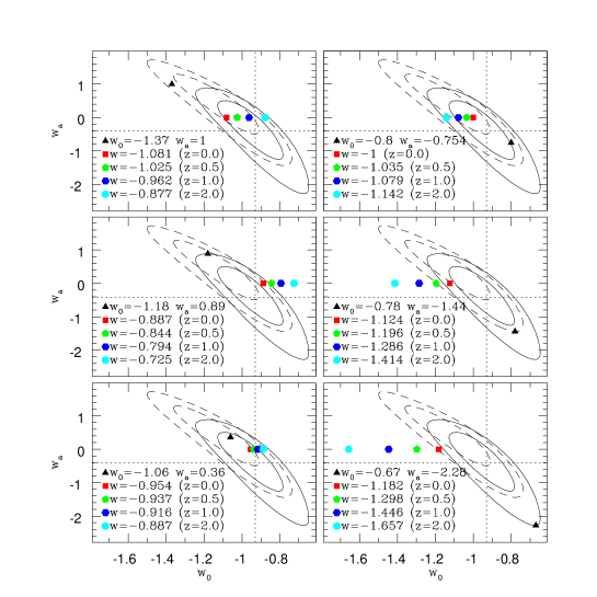
Figure 2: Each box refers here to a single $\cal A$ model in Figure 1 (black triangle) and related $\cal W$$(z)$ models (color polygones). Notice that, in most cases, distances between colored polygones are smaller than their distance from the black triangle. This outlines the possibility of a serious bias in data analysis, if data are tested by assuming constant–$w$ cosmologies.

The setting of the six $\cal A$ models considered is shown in the Figure. The other parameters are consistent with both WMAP5 and WMAP7 data: $\Omega_{m}=0.274$, $h=0.7$, $\sigma_{8}=0.81$ and $n_{s}=0.96$.

We test the spectra of $\cal A$ models vs. the corresponding $\cal W$$(z)$. All simulations start at $z=24$, from realizations fixed by an identical random seed. We use the pkdgrav code [6], modified to deal with any variable $w(a)$, as in [7]. In a box of side $L_{box}=256h^{-1}$Mpc we set $N=256^{3}$ particles and use a gravitational softening $\epsilon=25h^{-1}$kpc. We have 4 auxiliary models $\cal W$$(z)$ for $z=0,~{}0.5,~{}1,~{}2~{}$ (see Fig. 2), for each $\cal A$ model, run just down to the redshift where they are tested. For all models, mass functions agree with Sheth & Tormen [12] predictions.

The first $\cal A$ cosmology considered, consistent with WMAP5, is outside the 2–$\sigma$ curve for WMAP7. The significant shift of the ellipses is not due to the fresh CMB inputs. Rather, omitting the distance prior, as well as the whole SDSS data [8, 9], surely had an impact on it.

Figure 2 shows that the distance between $\cal W$ models, on the $w_{a}=0$ line by definition, is mostly smaller than their distance from $\cal A$. Distances depend on $w_{o}$ and are smaller for the central $w_{o}$ values. There is therefore a possible observational problem, as outlined in the Introduction.

Model spectra are worked out by FFT–ing the matter density field, computed on a regular grid $N_{G}\times N_{G}\times N_{G}$ (with $N_{G}=2048$) via a Cloud in Cell algorithm.

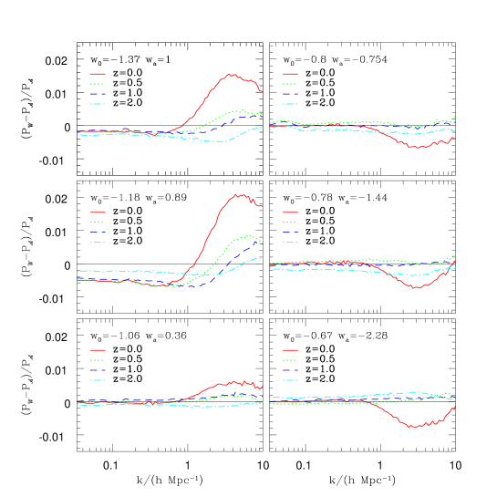
Figure 3: Spectral discrepancies at the redshift indicated by line colors. Each box refers to an $\cal A$ model with the same ordering as in Fig. 2. Top discrepancies at $z=0$; only there they approach $2\,\%$ for some model with $w_{o}\ll-1$ and for $k\sim 4$–$5\,h\,$Mpc^-1 (here however gas dynamics should not be ignored). Within $\sim 2$–$3\,h\,$Mpc^-1, discrepancies keep $<1\,\%~{}.$

Figure 3 then shows spectral discrepancies. Within $k=3\,h\,$Mpc^-1 the top discrepancy occurs for the two models with lowest $w_{o}$ ($<-1$), at $z=0$. Other models exhibit a nicer behavior, allowing to guess that the greatest discrepancies, between $\cal A$ and $\cal W$$(z=0)$ evolutionary histories, occur for models with $w_{o}\ll-1~{}.$ As expected, discrepancies decrease at higher $z$, where non–linearities had no time to affect low $k$’s. At $z=0.5$ they are in the permil range, for all models.

3 Hydrodynamical tests

We then compare $\cal A$ and $\cal W$$(z)$ models, also including baryon physics. Hydro simulations are much more time demanding and here we present results for one model: $w_{o}=-0.8,~{}w_{a}=-0.754\,$; top right in Figures 2 and 3. The assigned $\Omega_{m}$ value comes from $\Omega_{b}=0.046,~{}\Omega_{c}=0.228$.

The program used is gasoline, a multi-stepping, parallel Tree–smoothed particle hydro (SPH) n–body code [13]. It includes radiative and compton cooling. The star formation, based on [14], allows gas particles above constant density and temperature thresholds in convergent flows to spawn star particles at a rate proportional to the local dynamical time [15]. The program includes SN feedback [15] and a UV background, following [16]. We applied gasoline the same changes made in pkdgrav to handle dDE. Further details can be found in [7, 17].

All simulations use $(2\times)256^{3}$ particles and most are run in a box of 256$\,h^{-1}$Mpc. CDM (gas) particles have mass $m_{c}h/M_{\odot}=6.33\times 10^{10}$ ($m_{b}h/M_{\odot}=1.28\times 10^{10}$). The force resolution $\epsilon$ (softening) is 1/40 of the intra-particle separation. For $256\,h^{-1}$Mpc this yields $\epsilon\simeq 25~{}h^{-1}$kpc (wavenumber $\kappa=2\pi/\epsilon\simeq 150\,h\,$Mpc^-1). All simulations start at $z=24$. The $\cal A$ model is selected so that $\cal W$$(z=0)$ is $\Lambda$CDM. This $\Lambda$CDM was also run in a box of 64$\,h^{-1}$Mpc, still with $(2\times)256^{3}$ particles. All simulation parameters scale accordingly.

Figure 4 (l.h.s.) shows the ratios $M_{star}/M_{halo}$ vs. $M_{halo}$ in both 64 and 256$\,h^{-1}$Mpc boxes, compared with predictions in [18]. The Figure shows that star formation generally follows the halo occupation distribution trend. Slightly too many stars form in haloes in the top $M_{halo}$ bin, due to overcooling. This might be fixed by including AGN effects.

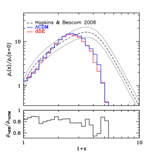
Figure 4: L.h.s.: Ratio between stellar and total mass in haloes. Empty and solid squares show the results for the 256 box; crosses for the 64 box. Results are compared with data in [18]; the 40% scatter yields $\sim\pm 2\sigma$. R.h.s.: Star formation evolution in $\Lambda{\rm CDM}$ and dDE in the 256 box; the dashed (black) line are data fits [19], assuming a Salpeter IMF; curves are normalized to the $z=0$ value. The lower panel shows the ratio between star productions in dDE and $\Lambda{\rm CDM}$ .

The r.h.s. of Fig. 4 shows star formation histories in 256$\,h^{-1}$Mpc boxes. Data [19] are also shown, with $\pm 20\,\%$ error bars, approximating 2-$\sigma$’s. Our outputs are shifted upwards by a factor 1.5 , so to account for an overall deficiency in star formation. Furthermore, observations and simulations peak for $z\simeq 2.3\,$ and $\simeq 1.5:$ stars form later in simulations. These discrepancies arise because stars do not form in halos with $<200$ gas particles [20], corresponding to a mass $\sim 1.3\times 10^{12}\,h^{-1}M_{\odot}$ in our simulations. In spite of that, at our resolution level star formation seems described well enough to allow spectral comparison on the scales relevant to us.

The bottom frame shows the ratio between star formation in $\cal A$ and $\Lambda$CDM. The decrease by $\sim 20\%$ arises from a change of $w(z),$ yelding a different evolutionary history, within an identical conformal age. Future work will seek the cause of this unexpectedly large shift.

Let us now come to spectral comparisons between $\cal A$ and $\cal W$$(z)$ models at $z=0$ and 0.5, 1, 2 . They are shown in Figures 5.

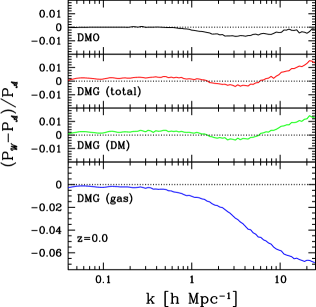
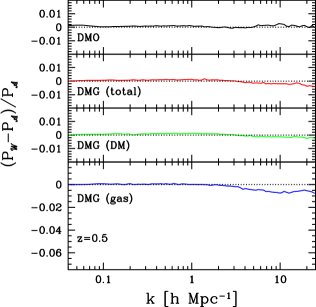
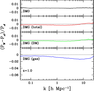
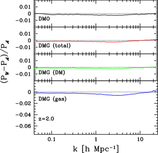
Figure 5: Comparison between $\cal A$ and $\cal W$$(z)$ spectra, for n–body (DMO) and hydro (DMG) simulations (various components shown). Top panels are for $z=0$ (l.h.s.) and $z=0.5$ (r.h.s.); bottom panels for $z=1$ and $z=2$.

For the model considered, regularities persist when gas dynamics is important, although residual discrepancies (mostly of the order of a few permils) are greater than in n–body simulations. The largest discrepancy is found in the gas spectra, even if the gas spectrum distortion at $z=0$, attaining $\sim 5\,\%$, apparently does not imply a significant distortion in the global spectrum.

Altogether we conclude that even the inclusion of hydrodynamics keeps the discrepancies between auxiliary and true model in the permil range, for the model considered.

4 References

References

- [1] Linder E V and Jenkins A, 2003 Mon. Not. R. Astron. Soc. 346 573
- [2] A. Refregier et al. , 2010, arXiv:1001.0061
- [3] Huterer D & Takada M, 2005 Astrophys. J. 23 369
- [4] Y.P. Jing, P. Zhang, W.P. Lin, L. Gao, V. Springel, 2006, APJ, L119
- [5] Francis M J, Lewis G F and Linder E V, 2007
- [6] Stadel J. G., 2001, PhD Thesis
- [7] Casarini L, Macciò A V & Bonometto S A, 2009 J. Cosmol. Astropart. Phys. 3 14
- [8] Komatsu E et al., 2009 Astrophys. J. Suppl. 180 330
- [9] Komatsu E et al., arXiv:1001.4538
- [10] Casarini L, Macciò A V, Bonometto S A, Stinson G., 2010, arXiv:1005.4683
- [11] Rudd D. H., Zentner A. R., Kravtsov A. V., 2008, Astrophys. J. , 672, 19
- [12] Sheth R. K., Tormen G., 2002, Mon. Not. R. Astron. Soc. , 329, 61
- [13] Wadsley J. W., Stadel J., Quinn T., 2004, NewA, 9, 137
- [14] Katz N., 1992, Astrophys. J. , 391, 502
- [15] Stinson G., Seth A., Katz N., Wadsley J., Governato F., Quinn T., 2006, MNRAS, 373, 1074
- [16] Haardt F., Madau P., 1996, Astrophys. J. , 461, 20
- [17] Governato F., Willman B., Mayer L., Brooks, A., Stinson G., Valenzuela O., Wadsley J., Quinn T., 2007, Mon. Not. R. Astron. Soc. , 374, 1479
- [18] Moster B. P., Somerville R. S., Maulbetsch C., van den Bosch F. C., Macciò A. V., Naab T., Oser L., 2010, Astrophys. J. , 710, 903
- [19] Hopkins A. M., Beacom J. F., 2006, Astrophys. J. , 651, 142
- [20] Christensen C., Quinn T., Stinson G., Bellovary J., Wadsley J., 2010, arXiv:1005.1681