Information filtering in complex weighted networks

Abstract

Many systems in nature, society and technology can be described as networks, where the vertices are the system’s elements and edges between vertices indicate the interactions between the corresponding elements. Edges may be weighted if the interaction strength is measurable. However, the full network information is often redundant because tools and techniques from network analysis do not work or become very inefficient if the network is too dense and some weights may just reflect measurement errors, and shall be discarded. Moreover, since weight distributions in many complex weighted networks are broad, most of the weight is concentrated among a small fraction of all edges. It is then crucial to properly detect relevant edges. Simple thresholding would leave only the largest weights, disrupting the multiscale structure of the system, which is at the basis of the structure of complex networks, and ought to be kept. In this paper we propose a weight filtering technique based on a global null model (GloSS filter), keeping both the weight distribution and the full topological structure of the network. The method correctly quantifies the statistical significance of weights assigned independently to the edges from a given distribution. Applications to real networks reveal that the GloSS filter is indeed able to identify relevant connections between vertices.

I Introduction

A popular way to look at a complex system is turning it into a graph, or network, by highlighting the fundamental elements of the system (vertices) and the interactions between them (edges connecting vertices), possibly with their strength (weights on edges). Due to the recent availability of massive data sets and computational facilities capable to process them, many networked systems have been carefully investigated in the last years albert02 ; boccaletti06 ; newman03 ; dorogovtsev01 ; pastor04 ; barrat08 ; caldarelli07 .

A recurrent property is the heterogeneity in the distributions of the main structural features of such systems. These include purely topological attributes, like the number of neighbors of a vertex (degree) albert99 ; Barabasi:1999 as well as variables depending on the weighted character of the edges, like the edge weights and the sum of the weights of the edges incident on a vertex (strength) Barrat:2004b . Such heterogeneity is responsible for peculiar properties of complex networks, like their high robustness against random attacks or failures cohen00 . Weights and topology are by no means independent, revealing a set of non-trivial relationships Barrat:2004b . For this reason it is improper to separate weights from topology and to study the system by exploiting either source of information.

However, keeping the full information about the network can give rise to problems. A large network with a high edge density may be intractable by traditional tools of network analysis. For instance, it may be impossible to produce a meaningful visualization of the network. Also, a high edge density is a serious obstacle for graph clustering techniques fortunato2010 , most of which rely on the working assumption that the network is sparse, i.e. that the number of edges is not much larger than the number of vertices. Other analysis tools may not be applicable due to their high computational complexity. In addition, the estimates of the edge weights may be biased by measurement errors, so the connections between some pairs of vertices might not be meaningful.

For all these reasons, it is important to develop suitable techniques to reduce the network, by maintaining only the most valuable information. The problem of information reduction in datasets has a long tradition and has led to the design of very popular methods, like Principal Component Analysis Jolliffe:2002 . For networked data a well known strategy is coarse graining Kim:2004 ; Itzkovitz:2005 ; song05 ; Gfeller:2007 , which consists in grouping vertices based on their mutual similarity or topological role in the network and replacing each group with super-vertices. Here, instead, we wish to preserve all vertices and act only on the edges, by selecting the most relevant ones. This is a major challenge. For one thing, it should be clarified what “relevant” means, as this is not straightforward. In fact, several options are possible, depending on the features of the system that shall be preserved. Since edge weights are usually broadly distributed, keeping just the largest weights is a viable option, since a few edges account for most of the total weight. All weights lower than a predefined threshold could be then erased farkas07 ; Eguiluz:2005 ; Allesina:2006 ; wu:2006 ; ramasco:2007 . However, global thresholding has two drawbacks. On the one hand, it introduces a scale in an originally multi-scale system. On the other hand it may spoil important topological properties. For instance, it may fragment the network into a large collection of components. To avoid that, one may construct a maximum spanning tree Macdonald:2005 , where as many edges as possible are removed such to maintain the connectedness of the graph and to keep the largest possible total weight on the remaining edges. This traditional technique is also not ideal, as it reduces the network to an acyclic graph (a tree), whereas cycles are very important structural features of complex networks. Moreover, a tree has a number of edges equal to the number of vertices minus one, and it is unlikely that the number of relevant edges simply depends on the number of vertices, for any system. Tumminello et al. have shown that many more edges/information can be kept, by extracting a subgraph that can be embedded on a surface of genus $k$, instead of a tree tumminello05 .

Still, selecting edges with a systematic bias towards the largest weights would destroy the heterogeneity in the distribution of edge weights, which is a crucial feature of complex weighted networks. Furthermore, this could significantly modify the coupling between weights and topology. Meanwhile there are a few methods capable to filter the information on the edges such to respect the multiscale structure of complex weighted networks. Such techniques include a two-stage algorithm proposed by Slater slater09 ; slater10 and a method by Glattfelder and Battiston glattfelder09 based on a multilevel network analysis. In recent works by Serrano et al. serrano09 ; serrano09a the focus is on the immediate neighborhood of each vertex. For a given vertex, the weights on its adjacent edges are analyzed, and those edges carrying a significant fraction of the total strength of the vertex are picked. The significance of the weight is estimated from the so-called disparity function, that results from a simple null model stating how weights are distributed among the edges incident on the vertex. Here we focus on the edges, i.e. on pairs of connected vertices, rather than on the individual vertices. Unfortunately, it is not possible to treat pairs of connected vertices independently of the rest of the network, as they are attached to other vertices, etc. The natural solution is a global null model, that accounts for the full topology of the network, while preserving the heterogeneity of the weight distribution. In this paper we propose the Global Statistical Significance (GloSS) filter, which satisfies these constraints.

At variance with other techniques, the GloSS filter yields a well defined global $p$-value for all edge weights of the network. Furthermore, it correctly identifies situations in which all edges are equally relevant/irrelevant, like when weights are independently and identically distributed on the edges. Finally, the performance of the GloSS filter on several real networks, both directed and undirected, is compared with that of other filtering techniques.

II Results and Discussion

II.1 The GloSS filter

The starting point is the weight matrix ${\bf W}$, whose element $w_{ij}$ indicates the weight of the edge joining vertices $i$ and $j$. If there is no edge/interaction between $i$ and $j$, $w_{ij}=0$. The number of neighbors of vertex $i$ is its degree $k_{i}$. We also recall that the strength Barrat:2004b $s_{i}$ of vertex $i$ is the sum of the weights of the edges incident on $i$: $s_{i}=\sum_{j}w_{ij}$. Our null model is a graph where the connections of the original network are locked, while weights are assigned to the edges by randomly extracting values from the observed weight distribution $P_{obs}\left(w\right)$. This null model thus preserves both the topology and the weight distributions of the original network, by construction.

Suppose that we want to evaluate the statistical significance, according to this null model, of the edge between vertices $i$ and $j$, with observed weight $w_{ij}$. The degrees and strengths of $i$ and $j$ are $k_{i}$, $k_{j}$, $s_{i}$ and $s_{j}$. This can be formalized by means of a Bayesian approach. The probability to observe weight $w_{ij}\neq 0$ on the edge, given the degrees and strengths of its endvertices, reads

$$P\left(w_{ij}\left|s_{i},k_{i},s_{j},k_{j}\right.\right)=P_{obs}\left(w_{ij}\right)\,\frac{P\left(s_{i},s_{j}\left|w_{ij},k_{i},k_{j}\right.\right)}{P\left(s_{i},s_{j}\left|k_{i},k_{j}\right.\right)}.$$ (1)

The denominator on the right hand side is a normalization factor, while $P_{obs}\left(w_{ij}\right)$ is a well defined number. In order to estimate the term in the numerator we must take into account that $w_{ij}$, $k_{i}$, $k_{j}$ are given and so the ”free” variables contributing to $s_{i}$ and $s_{j}$ are the weights of the remaining $k_{i}-1$ and $k_{j}-1$ connections of vertices $i$ and $j$, respectively. These weights can be treated as independent random variables in the null model, with the only restrictions that $\sum_{k\neq j}w_{ik}=s_{i}-w_{ij}$ and $\sum_{k\neq i}w_{jk}=s_{j}-w_{ij}$. This implies that

$$\begin{array}[]{ll}P\left(s_{i},s_{j}\left|w_{ij},k_{i},k_{j}\right.\right)=&F\left(s_{i}-w_{ij},k_{i}-1\right)\times\\ &F\left(s_{j}-w_{ij},k_{j}-1\right)\end{array}\;.$$ (2)

The function $F\left(s,k\right)$ is the probability of randomly extracting, from the weight distribution $P_{obs}\left(w\right)$, $k$ elements whose sum is equal to $s$, which means that

$$\begin{array}[]{ll}F\left(s,k\right)=&\int dx_{1}P_{obs}\left(x_{1}\right)\,\int P_{obs}\left(x_{2}\right)dx_{2}\cdots\\ &\cdots\int dx_{k}P_{obs}\left(x_{k}\right)\;\delta\left(x_{1}+x_{2}+\ldots+x_{k}-s\right)\end{array}\;,$$ (3)

where the Dirac delta $\delta\left(x_{1}+\ldots+x_{k}-s\right)$ ensures the satisfaction of the constraint on the vertices’ strength. We remark that, if either $i$ or $j$ (or both) has degree $1$, Eq. 2, as it stands, would not be defined. Here the whole strength of $i$ (or $j$) would come from the edge $ij$, so the probability distribution of observing that weight is just a $\delta$-function centered at $w_{ij}$, since no other values are compatible with the strength of the vertex ($s_{i,j}=w_{ij}$ if $k_{i,j}=1$).

Finally, the statistical significance (or $p$-value) $\alpha_{ij}$ of the observed edge weight $w_{ij}$ can be computed by calculating the integrals

$$\begin{array}[]{ll}\alpha_{ij}=P\left(>w_{ij}\left|s_{i},k_{i},s_{j},k_{j}\right.\right)=\frac{\int_{w_{ij}}^{\infty}dw\,P_{obs}(w)\,P\left(s_{i},s_{j}\left|w,k_{i},k_{j}\right.\right)}{\int_{0}^{\infty}dw\,P_{obs}(w)\,P\left(s_{i},s_{j}\left|w,k_{i},k_{j}\right.\right)}\end{array}\;.$$ (4)

Despite its apparently high complexity, the computation of the significance level can be carried out numerically in a fast and accurate way. The probability function $F\left(s,k\right)$ can in fact be viewed as a multiple convolution integral of the weight distribution function and its computation may be performed by invoking the convolution theorem. First the Fourier transform of the weight distribution is calculated, then its $k$-th power; the final answer is obtained by computing the Fourier antitransform of the result (see details in Appendix A). The extension of the former procedure to directed networks is straightforward. If $w_{ij}$ denotes the weight of the directed edge going from vertex $i$ to vertex $j$, it is sufficient to substitute in the former equations $k_{i}$ and $s_{i}$ with $k_{i}^{out}$ and $s_{i}^{out}$, respectively. For vertex $j$ one ought to replace $k_{j}$ with $k_{j}^{in}$ and $s_{j}$ with $s_{j}^{in}$. Once the $p$-value of each edge has been determined, we can establish a certain threshold and deem the edges as significant if their $p$-values lie above that threshold. This procedure defines what we have called the GloSS filter.

II.2 Tests on random weight distributions

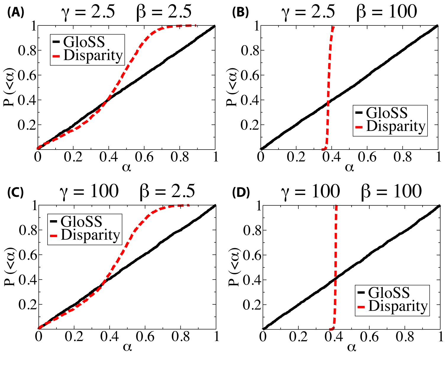
Ideally, any filtering procedure should be able to recognize situations in which there are no significant weights. For instance, given a distribution, we could assign weights taken from that distribution on each edge, independently of the other edges. In this way, the distribution of the weights on the edges would be random, with no correlations with topological features. Therefore, the fluctuations of the weights coming from such distribution are just the expected fluctuations of the distribution itself, whose statistical significance is exactly indicated by the $p$-value $\alpha$ of Eq. (4). The probability $P\left(<\alpha\right)$ for an observed weight to have a $p$-value $\alpha$ or lower is then exactly equal to $\alpha$, as all $p$-values are equally probable. In Fig. 1 we show the profile of $P\left(<\alpha\right)$ on random networks with power law distributions of degrees and weights, with exponents $\gamma$ and $\beta$, respectively. The four panels correspond to different choices of $\gamma$ and $\beta$. For high values of the exponents (like $\gamma,\beta=100$) the power law distribution is effectively exponential. In all cases we see that the GloSS filter recovers the expected relation $P\left(<\alpha\right)=\alpha$ (diagonal continuous line), which indicates that indeed weights are randomly distributed among the edges and there are no significant fluctuations. The Disparity filter by Serrano et al. serrano09 , instead, displays a different profile (dashed line). For actual power law distributions of weights (Figs. 1A and 1C), it yields the expected pattern up to a $p$-value of about $0.4$, then it deviates from it. In particular, for the case of exponential distributions of weights (Figs. 1B and 1D), all observed weights have essentially the same $p$-value $\alpha\simeq 0.4$ (yielding the approximate step function for the cumulative displayed in the figure). In this case the values of the weights are quite close to each other, and the method has problems to distinguish between them. We remark that, even if edge weights are quite homogeneous here, once their distribution is defined one can always assign to each weight a proper likelihood ($p$-value), and discuss about its compatibility with the chosen distribution. The different results obtained with the Disparity filter are due to the different null model adopted by this filter, which is local. However, at variance with the GloSS filter, it is not possible to build a network based on the null model of the Disparity filter, just because of its local character. It is only possible to restrict the picture to the subgraph consisting of a node and its incident edges.

Figure 1: (Color online) Cumulative distribution $P\left(<\alpha\right)$ of the significance level $\alpha$ for independent identically distributed weights. Networks are made of $N=1\,000$ vertices and have minimum degree equal to $5$. Connections among vertices are randomly drawn by preserving the a priori given degree sequence. Vertex degrees and edge weights are randomly chosen from the power law distributions $P\left(k\right)\sim k^{-\gamma}$ and $P\left(w\right)\sim w^{-\beta}$, respectively. Statistical significance of weights, for different choices of $\gamma$ and $\beta$, are computed with the GloSS filter (continuous curve) and the Disparity filter by Serrano et al. serrano09 (dashed curve).

Figure 2: (Color online) Top $50$ connections of the World Trade Web in year $2006$: GloSS filter (left), Disparity filter (right). Countries without edges are removed from the picture.

		GloSS					Disparity
rank		$\alpha$	$w$	start vertex	end vertex		$\alpha$	$w$	start vertex	end vertex
$1$		$3\times 10^{-7}$	$4649.2$	USA	Dominican Rep		$4\times 10^{-112}$	$307823$	USA	Canada
$2$		$1\times 10^{-6}$	$3893.1$	USA	Honduras		$1\times 10^{-62}$	$200515$	USA	Mexico
$3$		$3\times 10^{-6}$	$520.17$	Italy	Albania		$3\times 10^{-51}$	$211247$	Canada	USA
$4$		$5\times 10^{-6}$	$890.23$	Haiti	USA		$2\times 10^{-34}$	$4649.2$	USA	Dominican Rep
$5$		$2\times 10^{-5}$	$1176.9$	Zimbabwe	South Africa		$4\times 10^{-34}$	$38386.1$	USA	Venezuela
$6$		$3\times 10^{-5}$	$13084.3$	Belarus	Russia		$1\times 10^{-33}$	$13084.3$	Belarus	Russia
$7$		$6\times 10^{-5}$	$1263.25$	UK	Cyprus		$4\times 10^{-33}$	$82175.1$	China	Taiwan
$8$		$6\times 10^{-5}$	$727.11$	Uganda	Kenya		$8\times 10^{-30}$	$3893.1$	USA	Honduras
$9$		$6\times 10^{-5}$	$1580.3$	USA	Nicaragua		$3\times 10^{-28}$	$62399.9$	Austria	Germany
$10$		$8\times 10^{-5}$	$7572$	USA	Ecuador		$8\times 10^{-26}$	$315362$	USA	China
$11$		$9\times 10^{-5}$	$1642.65$	Benin	China		$9\times 10^{-26}$	$103930$	China	South Korea
$12$		$9\times 10^{-5}$	$3326.3$	USA	Guatemala		$9\times 10^{-26}$	$19399.3$	USA	Israel
$13$		$1\times 10^{-3}$	$4062.74$	Honduras	USA		$9\times 10^{-25}$	$7572$	USA	Ecuador
$14$		$1\times 10^{-3}$	$508.5$	USA	Haiti		$5\times 10^{-24}$	$143421$	Mexico	USA
$15$		$2\times 10^{-3}$	$1458.28$	Zambia	South Africa		$1\times 10^{-23}$	$38642.4$	Germany	Austria
$16$		$2\times 10^{-3}$	$187.33$	St. Kitts & Nevis	USA		$1\times 10^{-22}$	$106105$	Germany	Netherlands
$17$		$2\times 10^{-3}$	$2282.3$	USA	Sri Lanka		$5\times 10^{-22}$	$27804.6$	Germany	Czech Rep
$18$		$2\times 10^{-3}$	$1056.25$	Mozambique	South Africa		$1\times 10^{-21}$	$8822.4$	USA	Trinidad & Tobago
$19$		$2\times 10^{-3}$	$459.05$	India	Nepal		$4\times 10^{-21}$	$27330.9$	Ireland	UK
$20$		$2\times 10^{-3}$	$193.22$	China	Burkina Faso		$5\times 10^{-21}$	$19308.9$	Portugal	Spain

Table 1: List of the top $20$ most relevant connections of the World Trade Web according to the GloSS (left) and the Disparity filter (right), respectively. The weights are evaluated in millions of dollars. The edges selected by the Disparity filter carry on average much larger weights and have far lower p-values than those picked by GloSS.

II.3 Tests on real networks

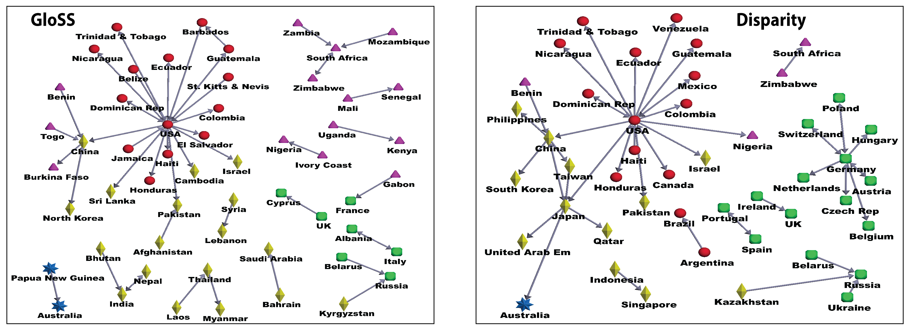
Here we show some applications of our filtering procedure to real weighted networks. First we focus our attention on the most “significant” weights of the network. For this purpose we take the World Trade Web (WTW) serrano03 , i.e. the network of trade relationships of world countries. Vertices represent the countries and edges are directed and weighted by the money flow running from any two countries to the other (import/export). The WTW is very useful to study propagation of economic crises and has been thoroughly investigated in the last years serrano03 ; garlaschelli04 ; garlaschelli05 . Data are freely available barbieri08 ; barbieri09 . The data we considered refer to the year $2006$: the network has $189$ vertices and $12\,705$ edges. In Fig. 2 we show the $50$ most significant edges, selected with the GloSS (left) and the Disparity (right) filter, respectively. We see that the results are quite different, even if some of the edges coincide. In particular, the GloSS filter is more likely to capture connections involving smaller/poorer countries than the Disparity filter, which selects more frequently larger countries and trade exchanges. This is manifest in Table 1, where we list the top $20$ edges, along with their weights and p-values.

Figure 3: (Color online) Applications of filtering techniques on two real weighted undirected networks: a network of US senators (left) and Zachary’s karate club (right). For each network we show the size of the largest connected component and the heterogeneity parameter of the degree ($k$), strength ($s$) and edge weight ($w$) distributions as a function of the number of edges added to the system (in decreasing order of relevance). The continuous line stands for the results of the GloSS filter, the dot-dashed line for those of the Disparity filter, the dashed line for global thresholding. In addition, we show scatter plots of the edge rankings estimated by the GloSS filtering technique and the other two considered here: Disparity and global thresholding.

Interesting economic relations, revealed as anomalous by the GloSS filter, are those between China and North Korea and also those relating China to Togo, Burkina Faso and Benin. While the existence of an anomalous connection between China and North Korea can be explained in terms of simple political reasons, the relations of China with the African countries have deeper economic foundations based on agreements on trade, economic and technological cooperation. Particularly relevant economic relations are also those established between Australia and Papua New Guinea, between Italy and Albania and between France and Gabon. Papua New Guinea became independent from Australia only in $1975$, but its economic development is still controlled by Australia. After the collapse of communism in Albania ($1991$), a mass exodus of refugees moved to Italy. Albanians form nowdays one of the largest foreign communities in Italy and strong trade relationships are present between the two countries. Gabon was a colony of France up to $1960$, but still maintain exclusive political and economic relationships with France.

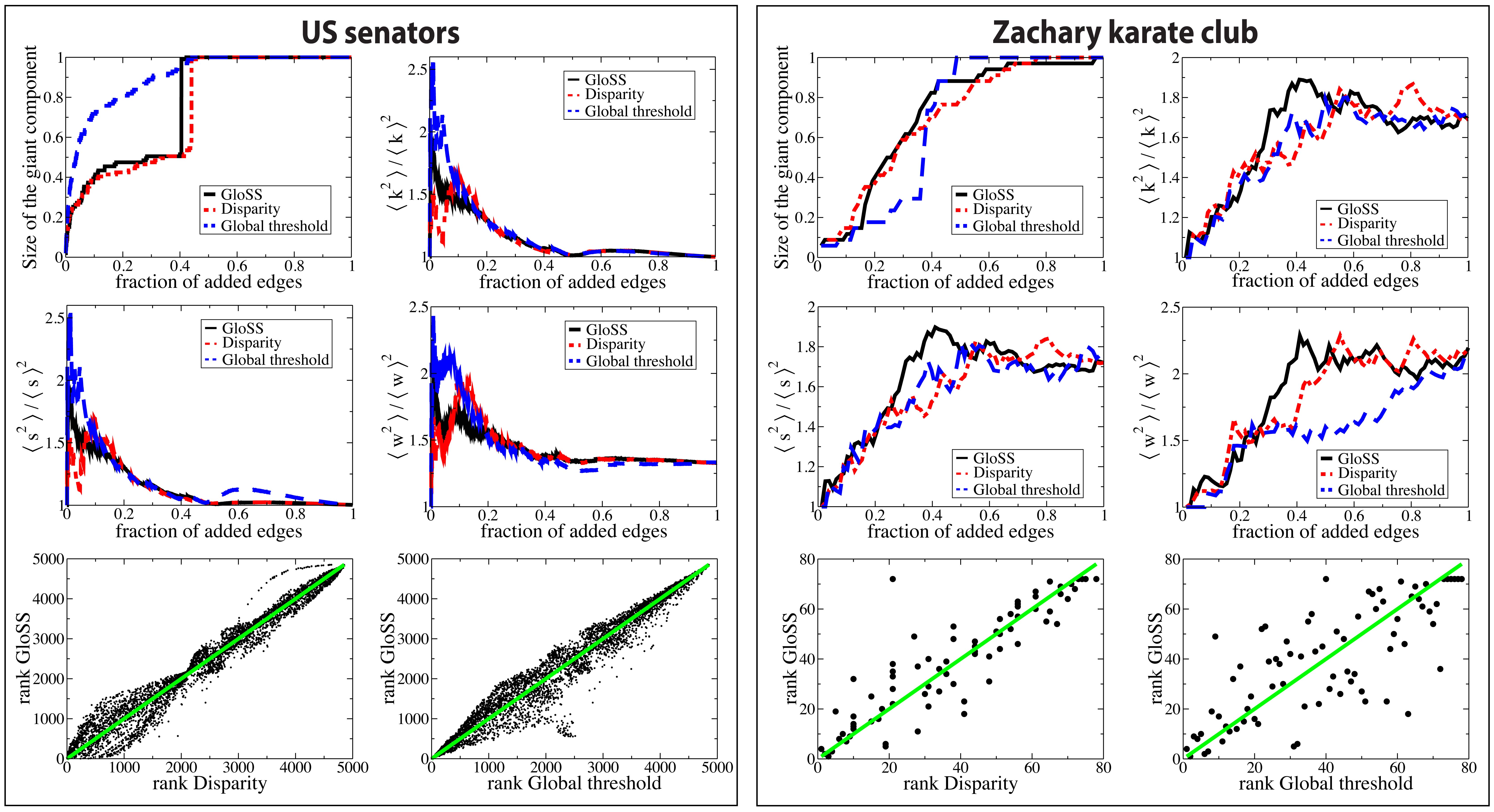
We now proceed with a more systematic study of the importance of the selected weights for the structure of the network. Since the goal is to reduce the information of the system by keeping as many as possible of its features, one may wonder how many edges, picked in descending order of significance, are necessary to reproduce the most important features of the original weighted graph. For instance, how many edges are needed to form a connected graph? This test has been suggested in Ref. serrano09 . In addition, we wish to check when the distributions of the vertex degrees, vertex strengths and edge weights are restored. Since it is hard to verify the match of two distributions, while it is far easier to compare two numbers, we limit the comparison to an important property of a distribution, the heterogeneity parameter, expressing the dispersion of the distribution around its average. For a variable $x$ with a certain probability distribution, the heterogeneity parameter is defined as the ratio of the second moment of the distribution by the square of the first moment: $\langle x^{2}\rangle/\langle x\rangle^{2}$. Our tests consist then in adding edges until the heterogeneity parameters of the distributions of the reduced network reach those of the original network and remain stable until the last edges are added. In Appendix B we use an alternative measure for the comparison of distributions: the Kullback-Leibler divergence kullback51 . We carried out the tests by using three different filtering techniques: GloSS, Disparity and global thresholding. We also compare the rankings produced by our filtering method with those obtained with the other techniques to estimate their correlation.

We start with two undirected graphs: a network of US senators poole07 and the karate club network of Zachary zachary . The first is a network with $99$ vertices, corresponding to members of the 109th Senate of the United States that served for the full two-years term. The weight of the edge between a pair of senators is weighted by the number of times they have voted in the same way (the total number of edges is $4\,851$). The data are freely available from http://voteview.com.

Figure 4: (Color online) Applications of filtering techniques on two real weighted directed networks: the US airport network (left) and the World Trade Web (right). The panels are analogous as those of Fig. 3, although those relative to the degree and strength distributions are split to account for the two possible edge directions (incoming and outgoing). The continuous line stands for the results of the GloSS filter, the dot-dashed line for those of the Disparity filter, the dashed line for global thresholding.

Naturally, senators of the same party (Republican or Democratic) are more likely to vote together than senators of different parties. Consequently, the distribution of edge weights is bimodal, with two groups of values corresponding to edges joining Republican or Democratic senators and to edges joining Republicans to Democrats. Zachary’s karate club network consists of $34$ vertices and $78$ edges, corresponding to the members of a karate club in the USA and their social relationships. It has become quite popular lately as it is frequently used as benchmark to test algorithms for community detection fortunato2010 . In Fig. 3 we show the results of our analysis of both graphs. The performances of the GloSS and Disparity filters are rather similar. For the senators network we see that after adding about $40\%$ of the edges the reduced network acquires the features of the original one. In this case, there is a strong correlation between the GloSS filter and global thresholding when it comes to selecting the most relevant edges. This is due to the fact that the senator network is almost fully connected and its weight distribution is bimodal (as opposed to the typically broad distributions observed in many systems). Under the null model assumption of random assignments of weights (from the given bimodal distribution), the larger weights between members of the same party are more likely to be deemed relevant by the GloSS filter.

Figure 5: (Color online) Applications of filtering techniques on two real weighted directed networks: the food web of Florida Bay in the dry season and the commuting network between cities in UK. The panels report the same analyses as those of Fig. 4. The continuous line stands for the results of the GloSS filter, the dot-dashed line for those of the Disparity filter, the dashed line for global thresholding.

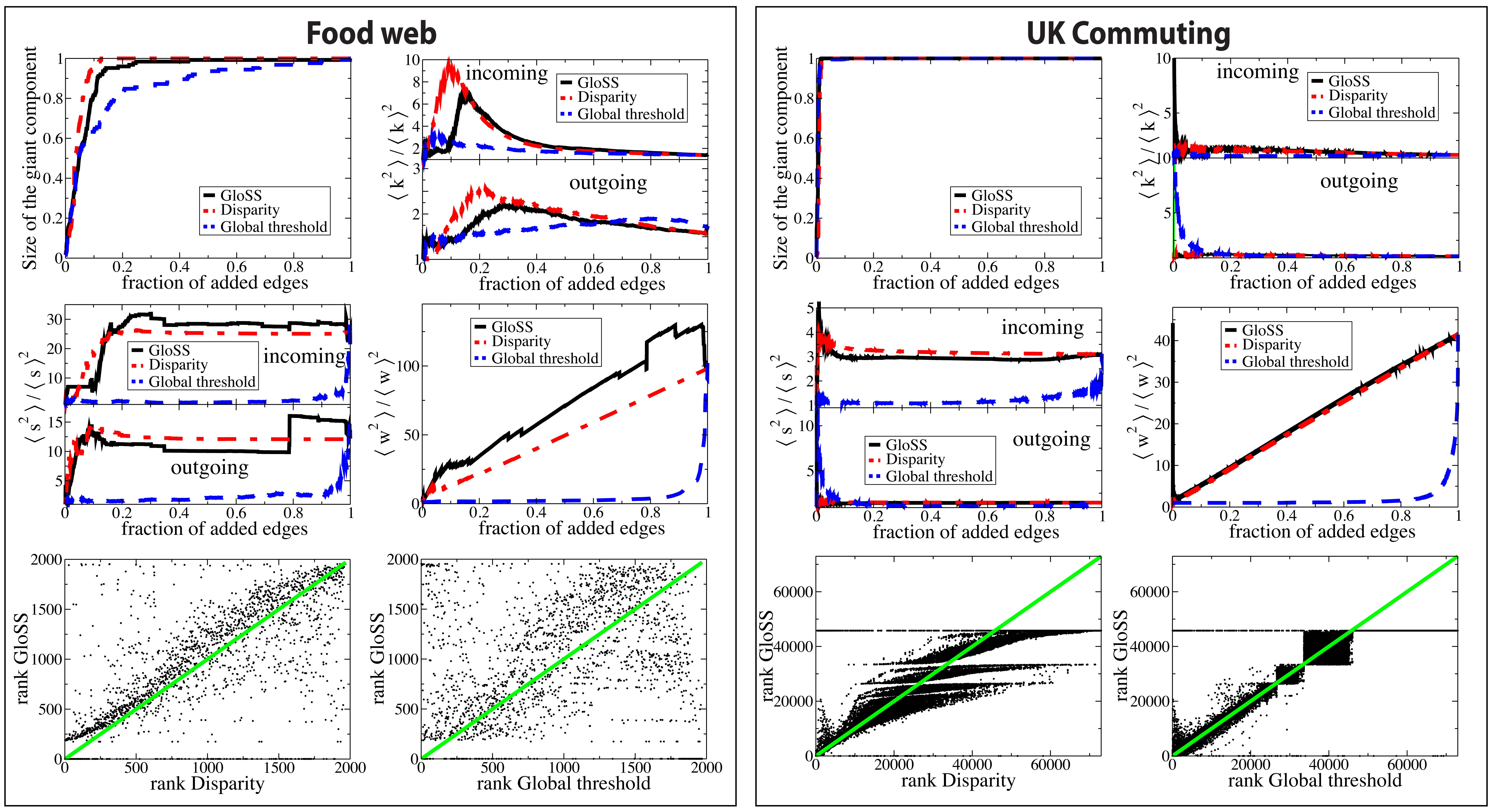
Finally, we discuss applications to directed networks. We take four datasets: the World Trade Web (WTW), the air transportation network of the USA, the Florida Bay ecosystem in the dry season ulanowicz98 and a network of commuting in the UK. The WTW has been described at the beginning of this subsection. Data on the US air transportation network can be downloaded from the Bureau of Transportation Statistics (US government) (http://www.bts.gov). Vertices are US airports and edges are weighted by the number of passengers transported along the corresponding routes in the year 2000. Our network has $664$ vertices and $15\,132$ edges. The food web of Florida Bay entails the trophic interactions between species, weighted by carbon transfers from one species to another. The network has been constructed within the ATLSS Project of the University of Maryland (http://www.cbl.umces.edu/atlss.html) The species are $125$, their interactions $1\,969$. The network of commuting is composed of $376$ vertices, representing local authorities, geographical divisions covering the territories of England and Wales. Each of the $72\,954$ directed edges corresponds to a flow of commuters between the local authority of origin and that of destination with a weight accounting for the number of commuters per day. The data come from the $2001$ UK census, where the local authority of residence and of work/study is registered for a significative part of the British population. The database can be accessed online at the site of the Office for National Statistics http://www.ons.gov.uk/census.

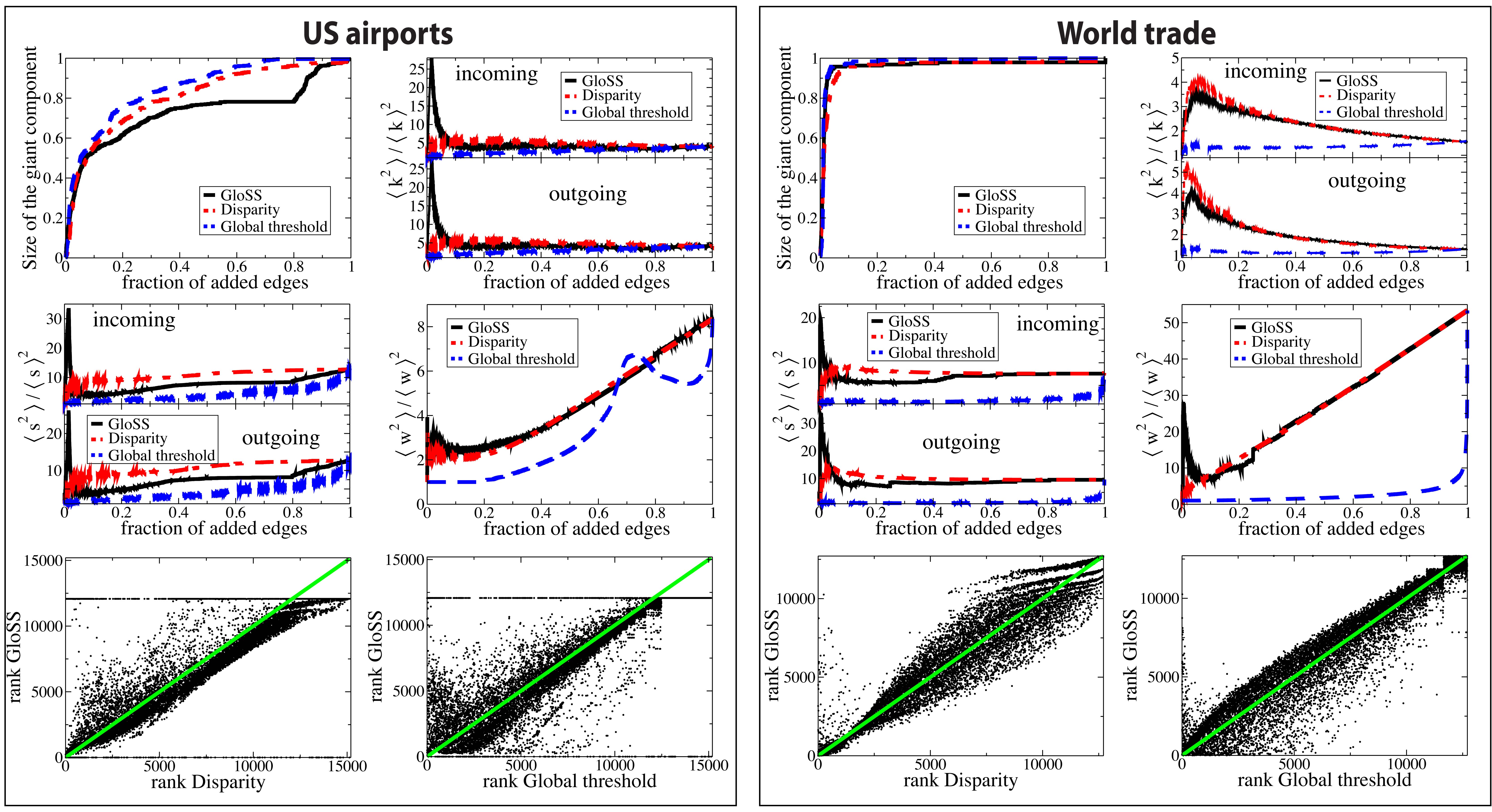
In Fig. 4 we show the results of our analysis for the WTW and the US airport network, following the same scheme as in Fig. 3. The results for the food web and the network of commuting are reported in Fig. 5. We remark again a substantial similarity between the GloSS and the Disparity filter. This seems to be odd, as the two filtering procedures are very different in their selection of the most significant edges, as we have shown in Fig. 2 and Table 1. What emerges from Figs. 3, 4 and 5 is that if a sizable fraction of edges are picked, both filters select mostly the same weights, so after a while the reduced descriptions of the network would match or become very similar. On the other hand global thresholding is clearly inadequate to catch the main properties of the original network, for it requires many more edges to recover them, as already pointed out in Ref. serrano09 .

Figure 6: (Color online) Cumulative distribution $P\left(<\alpha\right)$ of the significance level $\alpha$ for weights taken from the observed distribution of some of the real networks we considered. The continuous line corresponds to the GloSS filter, the dashed line to the Disparity filter.

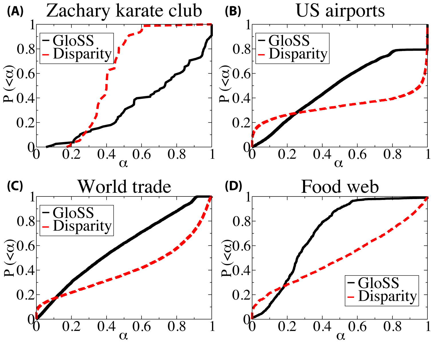
We close the section by performing a study analogous to that reported in Fig. 1, but for some of the real networks examined here (Fig. 6). For the GloSS filter (continuous lines) we find different patterns than that expected for the null model, in which all p-values are equally probable. Only for the US airports the p-values have roughly the same probability, up until $\alpha\sim 0.8$. For Zachary’s karate club, the WTW and the food web, there are significant differences with respect to the null model. The Disparity filter (dashed lines) displays a markedly different behavior: with the exception of Zachary’s karate club, very low $\alpha$ values are much more frequent than found by the GloSS filter.

III Conclusions

Filtering the information of complex weighted networks is crucial both to detect the most relevant connections and to be able to process a system that is often too large for many analytical tools to work efficiently. In this paper we have presented the first filtering technique based on a consistent global null model, preserving both the distribution of edge weights and the full topology of the graph. The recipe is by no means unique and it would not be difficult to propose alternatives with slight modifications of the main ingredients. In fact, filters are as arbitrary as the notion of “relevant information” is, so objective comparisons of different strategies are unfeasible. Still, there are situations in which the answer of the filter is intuitive. For instance, if weights are independently and identically distributed among the edges, there should be no anomalous fluctuations and, consequently, the $p$-values of the edges should be homogeneously distributed. We have seen that our GloSS filter indeed quantifies the correct statistical significance in such instances, while other techniques have problems.

Tests on real weighted networks show that the GloSS filter is capable of subsuming the basic information about the system in a fairly small fraction of the edges, especially the multiscale structure of both the topology and the edge weights. While we have put some emphasis on networks with heterogeneous distributions of features, we remark that our procedure is very general and it applies as well to cases in which distributions are peaked, as we have seen for the network of US senators. The significance of the edges is not so strongly correlated with their weights like for other techniques, so we are able to obtain potentially relevant information also from the vertices with low strength and degree and, consequently, a more balanced tradeoff between topology and weights.

Therefore we believe that the GloSS filter is a valuable tool for the analysis of networked datasets. The procedure is implemented in a freely downloadable software (http://filrad.homelinux.org/resources).

Appendix A Numerical implementation of the GloSS filter

The evaluation of the Fourier transform (and antitransform) can be performed by using a Fast Fourier Transform (FFT) algorithm. This requires as input a binned version of the weight distribution, where the number of bins $b$ must be a power of $2$. The range of values we are interested in is $\left[0,S\right]$, where $S=k_{max}w_{max}$ is the product of the maximal degree and the maximal weight observed in the network. A proper number of bins is needed in order to be able to distinguish different weight values: if $\delta w$ is the minimum value of the difference among all pairs of unequal weights in the network, we set $Q=\lceil\log_{2}\left(S/\delta w\right)\rceil$ and perform the linear binning of $P_{obs}\left(w\right)$ over $b=2^{Q}$ bins. We implement our filtering technique by calculating the Fourier transform of the weight distribution and all its powers up to $k_{max}$. For each resulting expression we obtain the Fourier antitransform and finally compute the $p$-values of all edges according to Eq. (4). The complexity of the various stages of our algorithm can be simply estimated: $b\,\log_{2}\left(b\right)$ is the typical complexity for calculating the Fourier transform or antitransform; computing the powers of the Fourier transform requires a time which grows as $b\,k_{max}$; deriving the inverse of the Fourier transform for each power scales as $k_{max}\,b\,\log_{2}\left(b\right)$; evaluating the statistical significance for each of the $M$ edges in the network goes as $M\,b$. Since in general $M\gg k_{max}$, the computational complexity of the whole filtering technique proposed in this paper is $M\,b=M\,2^{Q}$.

Appendix B Matching the backbone and the original graph

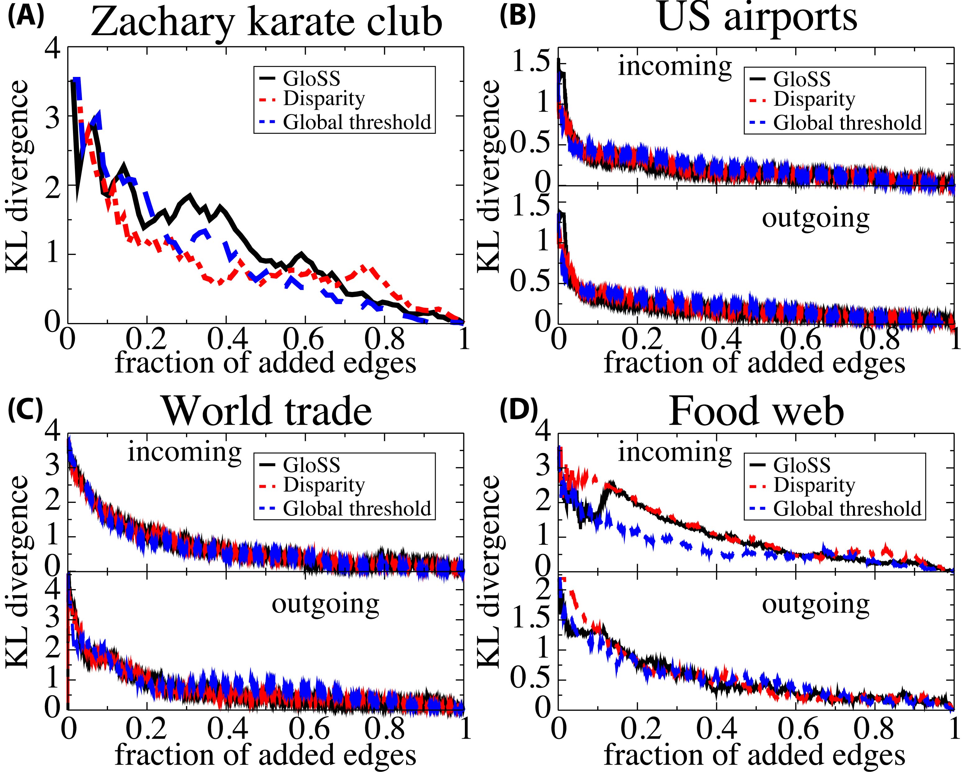
In Section II.3 we have compared the distribution of local properties of the backbone with that of the original graph, to check how many edges are needed to reproduce the basic features of the graph at study. For this purpose we have compared the heterogeneity parameters of corresponding distributions as a function of the fraction of added edges. To give more robustness to our results, we consider here an alternative measure for the comparison of distributions, the Kullback-Leibler (KL) divergence kullback51 , a well-known measure in information theory. The results are shown in Fig. 7 for four real networks. As we had found in Section II.3, there is little difference between the GloSS and the Disparity filters, while global thresholding follows slightly different trends.

Figure 7: (Color online) Each panel shows the difference between the degree distributions of the filtered networks and those of the original systems, measured by the Kullback-Leibler divergence, for the GloSS filter (continuous line), the Disparity filter (dot-dashed line) and global thresholding (dashed line). For directed graphs the panels are split in two halves, referring to the in-degree and the out-degree distributions, respectively.