Computing singularities of perturbation series

Abstract

Many properties of current ab initio approaches to the quantum many-body problem, both perturbational or otherwise, are related to the singularity structure of Rayleigh–Schrödinger perturbation theory. A numerical procedure is presented that in principle computes the complete set of singularities, including the dominant singularity which limits the radius of convergence. The method approximates the singularities as eigenvalues of a certain generalized eigenvalue equation which is solved using iterative techniques. It relies on computation of the action of the perturbed Hamiltonian on a vector, and does not rely on the terms in the perturbation series. Some illustrative model problems are studied, including a Helium-like model with $\delta$-function interactions for which Møller–Plesset perturbation theory is considered and the radius of convergence found.

I Introduction

Many-body perturbation theory (MBPT) has been one of the most popular approaches for ab initio many-body structure calculations, both in atomic, nuclear and chemical physics. Low-order Møller–Plesset (MP) partial sums were for many years considered highly accurate and the method of choice for calculations of ground state energies. However, in recent years it has become clear that the convergence properties are not that simple, and that plain MBPT more often than not is divergent Christiansen et al. (1996); Olsen et al. (1996); Dunning Jr. and Peterson (1998); Stillinger (2000); Leininger et al. (2000); Roth and Langhammer (2010).

Divergent series in this context can still be very useful. The series should be considered not as a final answer, but – as a Taylor series of a particular function with a particular singularity structure – be analyzed to obtain new ways of summing the series. Indeed the now extremely popular coupled cluster method, which has to a large extent supplanted low-order MBPT as the most effective method for ab initio structure calculations, can be described in terms of summations of selected classes of diagrams (i.e., selected terms in the series) to infinite order Bartlett (1981). Numerous other ways of resumming the series give improvements of the convergence, such as Padé or algebraic approximants Brändas and Goscinski (1970); Goodson (2000, 2003); Sergeev and Goodson (2006); Roth and Langhammer (2010). Especially in nuclear physics, summations of classes of diagrams to infinite order, such as the random-phase approximation Siu et al. (2009), have wide-spread use.

The performance of MBPT and the various resummation techniques is determined by the singularity structure of the energy eigenvalue maps $E_{n}(\lambda)$, where $\lambda$ is the perturbation parameter. The determination of these singularities, which are of branch-point type, is therefore crucial, but also very involved. Current approaches use the terms in the series to estimate the location of the singularities, perhaps in combination with approximants Hunter and Guerrieri (1980); Pearce (1978); Zamastil and Vinette (2005); Goodson (2000, 2003); Sergeev and Goodson (2006). However, due to a theorem by Darboux Pearce (1978); Sergeev and Goodson (2006) the asymptotic form of the series only gives information about the dominant singularity, i.e., the one closest to the origin, and such methods may also be sensitive to round-off errors Sergeev and Goodson (2006). It is also possible to do (very expensive) parameter sweeps of $\lambda$ to locate avoided crossings Helgaker et al. (2002); Sergeev et al. (2005); Herman and Hagedorn (2009), thereby discovering empirically some singularities, but only those with small imaginary parts.

In this article, we present a general and reliable numerical procedure for computing in principle the complete set of singularities of the eigenvalue maps $E_{n}(\lambda)$ and a procedure for determining the dominant singularity in standard Rayleigh–Schrödinger (RS) perturbation theory from the results, thereby finding the radius of convergence (ROC) of the series. The method relies solely on being able to compute the action of the Hamiltonian on a vector, which is compatible with the common approach of using the full configuration-interaction (FCI) methodology for computing the series terms Laidig et al. (1985); Handy et al. (1985); Christiansen et al. (1996); Olsen et al. (1996). We apply the numerical procedure to several examples and discuss the results.

We have chosen the examples for their instructive nature and the fact that we can compare with an explicit analysis. We analyze a simple harmonic oscillator with a $\delta$-function potential added Patil (2006), a three-electron quantum wire model in one spatial dimension Reimann and Manninen (2002), and an MP treatment of a Helium-like model with $\delta$-function interactions, which was also considered recently in detail by Herman and Hagedorn Herman and Hagedorn (2009) using parameter sweeps. In this paper we make conclusions about the ROC of this model. We use only very simple basis sets based on standard discretization techniques. The two first examples illustrate the properties of our numerical procedure, while the final example illustrates an application of moderate complexity.

Our method is based on the characterization of the singularities as branch points in the complex plane Kato (1995); Schucan and Weidenmüller (1973); Helgaker et al. (2002). Those are equivalently the points $\lambda_{*}$ where eigenvalues coalesce. It has been shown by the authors Jarlebring et al. (2010) that these points can be approximated to high precision by solving a particular two-parameter eigenvalue problem. More precisely, we find $\lambda(\varepsilon)$ such that a pair eigenvalues have a small relative distance $\varepsilon$, i.e., $E_{n}(\lambda)$ and $E_{m}(\lambda)=(1+\varepsilon)E_{n}(\lambda)$ are both eigenvalues. We adapt this result, exploit the structure of the Hamiltonian matrix, and combine this with modern solvers for eigenvalue problems.

The dominant singularity for RS perturbation theory for the ground state is the branch point $\lambda_{*,0}$ closest to the origin where $E_{0}$ meets $E_{n}$, $n\neq 0$ Schucan and Weidenmüller (1973); Kato (1995). The second part of the numerical method is a procedure that tracks the eigenvalue branches from the branch points $\lambda_{*}$ to the origin, thereby determining if it is the dominant branch point $\lambda_{*,0}$. We have chosen to focus on locating the dominant branch point since the ROC is a fundamental property of the perturbation series. The tracking procedure can equally well be applied to study other branch points.

After discussing the numerical method in Section II, we apply it to the model problems in Section III. Finally we present our conclusions in Section IV.

II Method

II.1 Properties of RS perturbation series

Consider a Hamiltonian matrix $H$ of dimension $N$ on the form

$$H(\lambda)=H_{0}+\lambda V,$$

where $V$ is treated as a perturbation, and where $\lambda$ is a complex parameter introduced for convenience. For the actual physical system we have $\lambda=\lambda_{\text{phys}}\in\mathbb{R}$. Both $H_{0}$ and $V$ are Hermitian matrices. The eigenvalues $E_{n}(\lambda)$ of $H(\lambda)$ are the $N$ roots of the characteristic polynomial $\det[H(\lambda)-EI]$, where $I$ is the identity matrix. The eigenvalues $E_{n}(\lambda)$ are the branches of an $N$-valued algebraic function, whose only singular points (denoted $\lambda_{*}$) are in fact of branch-point type Kato (1995); Schucan and Weidenmüller (1973); Helgaker et al. (2002).

For Hermitian matrices the branch-points come in complex conjugate pairs. There are no real branch points, and in the generic case (see Section II.4) all branch points are of square-root type. For sufficiently small $\lambda-\lambda_{*}$ the eigenvalues can be expanded in a Puiseux series around each branch point Schucan and Weidenmüller (1973). This is contained in Katz’ theorem Katz (1962) which we state here:

Theorem 1

Suppose $H(\lambda)=H_{0}+\lambda V$ is generic in the sense that $H_{0}$ and $V$ are Hermitian and chosen at random. Then for any pair of branches $E_{n}$ and $E_{m}$ there exists a branch point $\lambda_{*}$ at which $E_{n}(\lambda_{*})=E_{m}(\lambda_{*})=b_{nm}$. Moreover, for sufficiently small $\lambda-\lambda_{*}$ there exists a constant $c_{nm}$ such that

$$E_{n}(\lambda)=b_{nm}+c_{nm}(\lambda-\lambda_{*})^{1/2}+\mathcal{O}(\lambda-\lambda_{*})$$

and

$$E_{m}(\lambda)=b_{nm}-c_{nm}(\lambda-\lambda_{*})^{1/2}+\mathcal{O}(\lambda-\lambda_{*}),$$

where it is to be understood that the same branch of the square-root function is to be used in both equations.

Katz’ theorem may be viewed as a generalization of the well-known Wigner–von Neumann non-crossing rule Schucan and Weidenmüller (1973). It is interesting that all eigenvalue pairs are involved at some branch point, which implies that the function $E_{0}(\lambda)$ actually can be analytically continued to any excited state $E_{n}(\lambda)$.

Finite-dimensional Hamiltonians usually arise due to some discretization in form of a finite basis set, e.g., using the FCI methodology. The singularity structure of the full problem is richer than in the finite-dimensional case, but we postpone a brief discussion to Section III.1.

In RS perturbation theory for the ground state one computes a truncated Taylor series for $E_{0}(\lambda)$, viz,

$$E_{0}(\lambda)=\sum_{k=0}^{K}E_{0,k}\lambda^{k}+\mathcal{O}(\lambda^{K+1}),$$

which is an asymptotic series approximating $E_{0}(\lambda)$ as $\lambda\rightarrow 0$. The coefficients $E_{0,k}$ can be generated recursively by insertion into the eigenvalue problem for $H(\lambda)$ which gives a series usually represented in form of Feynman diagrams. The actual computation of the terms become increasingly complicated for higher-order terms for many-body systems (in practice, one rarely computes more than sixth-order series using diagrammatic techniques), but if $H(\lambda)$ is is available as a matrix or as a procedure that computes matrix-vector products, the high-order terms are straightforward to compute Laidig et al. (1985); Roth and Langhammer (2010).

One of the important questions we consider in this paper is whether the truncated series is convergent as $K\rightarrow\infty$ for $\lambda=\lambda_{\text{phys}}$, that is to say whether the ROC is greater than $\lambda_{\text{phys}}$ or not. As a Taylor series, the ROC is given by $|\lambda_{*,0}|$, where $\lambda_{*,0}$ is the smallest branch point, called the dominant branch point, where the branch belonging to $E_{0}(0)$ meets a different branch $E_{n}$, $n\neq 0$. We say that the $E_{0}$ and $E_{n}$ branch at $\lambda_{*,0}$ Kato (1995); Baker (1971); Schucan and Weidenmüller (1973); Goodson and Sergeev (2004). We remark that in other perturbation theories, like the folded diagram series for the effective interaction in nuclear physics Schucan and Weidenmüller (1973), other branch points may be dominant.

Thus, to compute the dominant singularity we are looking for the points $\lambda_{*}\in\mathbb{C}$ not on the real line such that $E_{n}(\lambda_{*})=E_{0}(\lambda_{*})$ for $n\neq 0$. The ROC is then $R=\min\{|\lambda_{*}|\}=|\lambda_{*,0}|$. Instrumental to this we consider the values of $\lambda$ such that the matrix $H(\lambda)=H_{0}+\lambda V$ has a double eigenvalue. In what follows we call such a value of $\lambda$ a critical value. It usually is a branch point, but in some cases we also get spurious solutions.

II.2 Computing the $m$ smallest critical values

We saw above that it is possible to characterize the singularities of a perturbation series by computing $\lambda$ such that $H(\lambda)$ has a double eigenvalue. The problem of finding all $\lambda$ such that a matrix depending linearly on $\lambda$ has a double eigenvalue has been considered by the authors elsewhere Jarlebring et al. (2010). The derivation of the method presented here is based on a result in Ref. Jarlebring et al. (2010) stating that all solutions can be approximated by the solutions of a generalized eigenvalue problem defined as follows. We let $\varepsilon>0$ be a small scalar, called the regularization parameter, and define the matrices $\Delta_{0}(\varepsilon),\,\Delta_{1}(\varepsilon)\in\mathbb{C}^{N^{2}\times N^{2}}$ by

$$\Delta_{0}(\varepsilon)=-I\otimes V+(1+\varepsilon)V\otimes I$$

and

$$\Delta_{1}(\varepsilon)=I\otimes H_{0}-(1+\varepsilon)H_{0}\otimes I,$$

where $\otimes$ denotes the Kronecker product. Consider now the generalized eigenvalue problem

$$\lambda\Delta_{0}(\varepsilon)v=\Delta_{1}(\varepsilon)v,\ \ \$$ (1)

where $v=v_{1}\otimes v_{2}$. An important result is is that the solutions of (1) approximate all $\lambda$ such that $H(\lambda)$ has a double eigenvalue.

Approximations of the eigenvalues $E_{n}(\tilde{\lambda})$ can be obtained from the eigenvalue problem for the matrix $H_{0}+\tilde{\lambda}V$, where $\tilde{\lambda}$ satisfies (1). To shed a light on this approach, one can prove that the eigenvalues of (1) correspond to the set of values of $\lambda$ for which the matrix $H_{0}+\lambda V$ has two eigenvalues within a relative distance of $\varepsilon$, i.e., a pair of eigenvalues of the form $E$ and $E(1+\varepsilon)$. This is clearly a relaxation of the problem. A suitable choice of $\varepsilon$, as well as other implementation aspects, have been studied in detail Jarlebring et al. (2010). This includes the exclusion of spurious solutions. It is also showed that the error in $\tilde{\lambda}$ behaves like $\mathcal{O}(\varepsilon^{2})$.

Although the above method allows us to compute all critical values of $\lambda$, it may be computationally prohibitive for large problems. The computational complexity is determined by the solution of the generalized eigenvalue problem (1), which requires $\mathcal{O}(N^{6})$ operations if all eigenvalues are computed with a general purpose method. To overcome this problem we use an iterative method known as the Arnoldi method Saad (1992), to compute the $m$ smallest eigenvalues of (1), where $m$ is a given integer.

The Arnoldi method generalizes the familiar Lanczos iterations employed in FCI calculations to non-Hermitian matrices, and only requires an efficient computation of the matrix-vector product associated with the eigenvalue problem. The matrix-vector product associated with (1) is

$$y=\Delta_{1}(\varepsilon)^{-1}\Delta_{0}(\varepsilon)x.$$ (2)

Let $X,Y\in\mathbb{C}^{N\times N}$ be such that $x=\operatorname{vec}(X)$ and $y=\operatorname{vec}(Y)$, where $\operatorname{vec}:\mathbb{C}^{N\times N}\rightarrow\mathbb{C}^{N^{2}}$ denotes the vectorization operation, i.e., stacking the columns of the matrix on top of each other. A key to the success of our method is that we can express the matrix-vector product (2) in terms of the matrices $X$ and $Y$. By straightforward manipulations using the rules of the Kronecker product we obtain

$$H_{0}Y-(1+\varepsilon)YH_{0}^{T}=-VX+(1+\varepsilon)XV.$$ (3)

This matrix equation, where $Y$ is the unknown, is a matrix equation known as a Sylvester equation. The right-hand side can be evaluated in $\mathcal{O}(N^{3})$ operations. The Sylvester equation can be solved in $\mathcal{O}(N^{3})$ operations by using the Bartels-Stewart algorithm Bartels and Stewart (1972), which is a standard method for Sylvester equations. Hence, by exploiting the structure in this way, the matrix-vector products of (1) can be efficiently computed in $\mathcal{O}(N^{3})$ operations. If $H_{0}$ is diagonal, this can be improved to $\mathcal{O}(N^{2})$ operations, which is seen as follows.

Let $Y=:(y_{1},\ldots,y_{N})$ and $(c_{1},\ldots,c_{N})$ the columns of the right-hand side of (3). Suppose the diagonal entries of $H_{0}$ are $H_{0,i,i}$,  $i=1,\ldots,N$. It is straighforward to show that column $i$ of (3) can be written as the solution of a linear system with a diagonal matrix,

$$y_{i}=\operatorname{diag}(d_{1},\ldots,d_{N})c_{i}$$ (4)

where

$$d_{j}=\frac{1}{H_{0,j,j}-(1+\varepsilon)H_{0,i,i}},\;j=1,\ldots,N.$$

Now note that we can compute a column vector of $Y$ using (4) with only $\mathcal{O}(N)$ operations. Hence, the Sylvester equation corresponding to diagonal $H_{0}$ can be solved in $\mathcal{O}(N^{2})$ operations. In the simulations in Section III.3 we will use this approach, whereas using the Bartels-Stewart algorithm Bartels and Stewart (1972) turned out to be more robust in Section III.4.

Two additional properties of the Arnoldi method makes it particularly suitable for our purposes.

• As we shall illustrate in Section III the overall algorithm for computing the dominant branch point, outlined in Section II.3, typically requires only a small number of critical values $m\ll N$. The Arnoldi method can be useful if not all eigenvalues need to be computed.

• If the chosen $m$ is deemed insufficient, we wish to continue the iteration. The Arnoldi method can be easily resumed if more eigenvalues are needed.

The procedure above describes a method which can be used for quite large systems since the complexity of the matrix-vector product is only $\mathcal{O}(N^{2})$. The matrices $V$ and $H_{0}$ stem from discretizations and we wish to be able to solve as large systems as possible. We will now use that for large problems (fine discretization/large basis set), a somewhat accurate guess is available by solving a corresponding smaller problem (coarser discretization/small basis set).

Inverse iteration Saad (1992) is a method to compute one eigenpair where a reasonable approximation of the eigenvalue is already available. Inverse iteration is, similar to the Arnoldi method, also only based on matrix vector products. It however, does not involve any orthogonalization step. Since it is only based on matrix-vector products we can use (3) directly with inverse iteration.

By using the Arnoldi method for a coarse discretization, and inverse iteration for a finer discretization, we can solve very large problems in a reliable way in a multi-level fashion.

II.3 Computing the dominant branch point

The value $\lambda_{*,0}\in\mathbb{C}$ is the first branch point of $E_{0}(\lambda)$. Since $H(\lambda_{*,0})$ has a double eigenvalue, we can compute candidates for $\lambda_{*,0}$, i.e. the critical values, with the procedure described in Section II.2. It now remains to determine which one of the candidate solutions computed with the method in Section II.2 corresponds to $\lambda_{*,0}$.

We will use a computational approach based on following paths from the candidate solution $\lambda$ to the origin. It is justified by the following technical result.

Proposition 2

Consider a critical value $\tilde{\lambda}$ such that $|\tilde{\lambda}|<|\lambda_{*,0}|$. Let $p:[0,1]\rightarrow\mathbb{C}$ be a parametrization of a curve from $p(0)=\tilde{\lambda}$ to $p(1)=0$ such that $|p(\theta)|\leq|\tilde{\lambda}|$ for $\theta\in[0,1]$. Assume that $p$ does not pass directly through another critical value. Then two continuous eigenvalue functions $[0,\ 1]\ni\theta\mapsto E_{n}(\theta)$ and $[0,\ 1]\ni\theta\mapsto E_{b}(\theta)$ satisfying $E_{a}(\theta),E_{m}(\theta)\in\sigma(H_{0}+p(\theta)V)$ for $\theta\in[0,\ 1]$ and $E_{n}(0)=E_{m}(0)$ are uniquely defined. Moreover, we have

$$E_{n}(1)\neq E_{0}(0)\textrm{ and }E_{m}(1)\neq E_{0}(0).$$

Proof. The first statement follows from Rouché’s Theorem Krantz (1999). The second statement can be proven by contradiction. More precisely, the statement $E_{n}(1)=E_{0}(0)$ or $E_{m}(1)=E_{0}(0)$ contradicts with the assumption $|\tilde{\lambda}|<|\lambda_{*,0}|$. $\Box$

From Proposition 2 it follows that $\lambda_{*,0}$ is the smallest branch point for which one of the corresponding curves, $E_{n}$ or $E_{m}$, terminates at $E_{0}(0)$. Only the branch points with positive (or negative) imaginary parts are relevant and some may be spurious. Denoting all relevant numerical branch points by $\left\{\lambda_{k}\right\}_{k=1}^{N^{\prime}}$, where

$$|\lambda_{1}|\leq|\lambda_{2}|\leq\ldots\leq|\lambda_{N^{\prime}}|,$$

this brings us to the following algorithm.

Algorithm 3

(Computation of the ROC)

• Compute $E_{0}(0)$, set $i=1$.

• Consider $\lambda_{i}$ and continue the two corresponding branches $E_{n}$ and $E_{m}$ for $\theta\in[0,\ 1]$, i.e. from $\lambda=\lambda_{i}$ to $\lambda=0$.

• If one of the branches terminates at $E_{0}(0)$, then stop
  else $i=i+1$, go to step 2.

• $R=|\lambda_{i}|$.

We conclude this section with some implementation aspects. For step 2. critical values of the parameter $\lambda$ are needed in increasing magnitude. These can be computed by the Arnoldi algorithm as described in Section II.2. The value of $m$ is fixed before the iteration starts. If it turns out to be insufficient, the Arnoldi process can still be resumed as also outlined in Section II.2.

For the continuation process in step 3. we assume that curve $p$ is linear, i.e. the curve corresponding to $\lambda_{i}$ satisfies

$$p(\theta)=(1-\theta)\lambda_{i}.$$

As the critical values are isolated points, this line does not contain other critical values, with probability one. For the continuation of the eigenvalues we follow the eigenvalues by sampling the line between $\theta\in[0,1]$ with sufficiently many points. In our applications, $21$ sampling points were sufficient to follow the eigenvalues accurately and not dominate the computation time.

Although we have chosen to to so in our implementation, it is not necessary to compute the whole set of eigenvalues along $p(\theta)$. Standard continuation techniques may instead be used, where continuity of the eigenvalues with respect to $\theta$ is exploited. See for example the book by Seydel Seydel (2010).

II.4 A comment on genericity

As stated in Section II.1 the statements concerning the nature and location of the branch points $\lambda_{*}$ of the eigenvalue maps depend on the fact that $H(\lambda)$ is generic: a statement indicating that the matrix is a “typical” Hermitian matrix. Statements about generic matrices hold with probability $1$ when the matrix is chosen at random.

On the other hand, Hamiltonians are rarely generic: symmetries such as angular momentum conservation or parity invariance lead to a natural block structure in $H(\lambda)$ so that the eigenvalue problem decouples into smaller, unrelated problems. It is easy to see that the non-crossing rule may be violated, and consequently that not all critical points of $H(\lambda)$ are branch points if not all symmetries are removed from the system. The numerical procedure then yields spurious real or complex solutions corresponding to violations of the non-crossing rule or the square-root branch point classification, respectively.

III Numerical results

III.1 Branch points in complete basis limit

In this section we apply the numerical procedure to three model problems: a simple one-dimensional harmonic oscillator with a $\delta$-function spike, which is exactly solvable Patil (2006) and equivalent to a center-of-mass frame formulation of a parabolic two-electron quantum wire with $\delta$-function interactions, a three-electron parabolic quantum wire with smoothed Coulomb interactions Reimann and Manninen (2002), and a helium-like model with $\delta$-function nuclear and inter-electron interactions Herman and Hagedorn (2009). In the latter example we consider Møller–Plesset perturbation theory, while in the other examples we let the perturbation $V$ be the bare inter-particle interactions.

The Hamiltonian matrix is like in most MBPT approaches an approximation of a partial differential operator $\mathcal{H}$ obtained by a finite basis expansion with discretization parameter $h$, i.e., as $h\rightarrow 0$, the dimension $N\rightarrow\infty$ and the discrete spectrum approaches the exact limit under mild conditions. (Special care has to be taken for the continuum spectrum of $\mathcal{H}$ if it exists.)

One may characterize the singularities of the eigenvalue map of $\mathcal{H}$ as $\alpha$ or $\beta$ singularities Goodson (2003). The $\alpha$ singularities are complex-conjugate pairs of branch points with non-zero imaginary parts. These are also called “intruder states” Helgaker et al. (2002). A finite-dimensional Hamiltonian only has $\alpha$ type branch points. The $\beta$ singularities are real branch points corresponding to a coalescence of an eigenvalue with the continuous spectrum. Baker argued this is a generic feature of unconfined fermion systems Baker (1971); Goodson and Sergeev (2004); Herman and Hagedorn (2009). The approximate Hamiltonian will, as long as it contains sufficiently good approximations to continuum states, have a cluster of branch points near a $\beta$ singularity. As $h\rightarrow 0$, assuming that the basis set is in fact complete, the continuous spectrum is “filled out” with discrete points, and hence there will be many close crossings clustering around (but never equal to) a real value.

To interpret and classify the numerically found $\lambda_{*}$ we must consider the non-trivial limit $h\rightarrow 0$. In general, three cases can be expected:

1. The branch point approaches a finite, complex value, and represents an $\alpha$ singularity.

2. The branch point approaches infinity, in case of which a singularity of the perturbation series disappears for the exact Hamiltonian.

3. The branch point approaches a finite real value. This can happen in two separate ways: (i) Since the branch points come in complex conjugate pairs this means that the limit actually becomes an analytic point as $h\rightarrow 0$, i.e., a violation of the non-crossing rule (which does not hold in the infinite-dimensional case). (ii) The real limit corresponds to a $\beta$ singularity. In that case infinitely many branch points must approach the same real value as $h\rightarrow 0$ ($N\rightarrow\infty$).

III.2 Harmonic oscillator with $\delta$-function

We consider the toy model Hamiltonian Patil (2006)

$$\mathcal{H}(\lambda)=-\frac{1}{2}\frac{\partial^{2}}{\partial x^{2}}+\frac{1}{2}x^{2}+\lambda\delta(x).$$

Any fixed $\lambda=\lambda_{\text{phys}}$ may be taken as the actual, physical value for the toy model.

The eigenvalue problem $(\mathcal{H}-E)\psi(x)=0$ may be solved to arbitrary precision and represents a particularly instructive test-case for our numerical procedure. Parity symmetry allows us to focus on even eigenfunctions which includes the ground state. (The odd eigenfunctions are in fact trivial since $\delta(x)\psi(x)=0$ in this case.) Figure 1 shows the eigenvalues of the even eigenfunctions as $\lambda$ is varied.

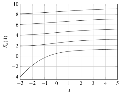
Figure 1: Eigenvalues of the harmonic oscillator with a $\delta$-function. Only eigenvalues of even eigenfunctions are shown. Notice the crossing with the real axis around $\lambda\approx-0.6758$, which will give rise to a spurious solution in the numerical method.

Introducing the even-numbered harmonic oscillator basis functions $u_{n}(x)=\phi_{2n}(x)$ we obtain $(H_{0})_{nm}=(2n+1/2)\delta_{nm}$ and $V_{nm}=\phi_{2n}(0)\phi_{2m}(0)$, the latter being a rank 1 matrix. Here,

$$\phi_{n}(x)=(2^{n}n!\sqrt{\pi})^{-1/2}H_{n}(x)e^{-x^{2}/2},$$ (5)

with $H_{n}(x)$ being the standard Hermite polynomials. It has been shown Jarlebring et al. (2010) that the numerical procedure will give spurious solutions of large magnitude since $V$ has rank one; in this case $|\lambda_{*}|\sim 10^{12}$. Also, one false real value arises for $\lambda$ such that $H(\lambda)$ has a zero eigenvalue, see Figure 1. Note that all spurious solutions are easily detected.

Figure 2 shows the smallest computed branch points for various $N$ with the dominating $\lambda_{*,0}$ inset. The results for the various $N$ indicate that the qualitative distribution of branch points does not change much with the basis size. For $N\rightarrow\infty$ we then estimate that RS perturbation theory will converge for all $|\lambda|<2$.

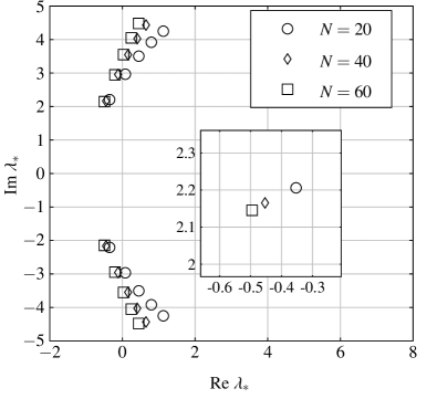
Figure 2: The smallest branch points for the harmonic oscillator with a $\delta$-function, computed for various matrix sizes $N$. The dominating branch point $\lambda_{*,0}$ is shown inset.

We remark that it is not easy to find the branch points by doing a parameter sweep. Figure 1 does not reveal clear avoided crossings involving any pairs of eigenvalues, which is explained by the large imaginary parts of the various $\lambda_{*}$.

We conclude this subsection by plotting the paths the eigenvalues trace out when $\lambda$ is gradually decreased from $\lambda_{*}$ to zero, i.e., we consider $\lambda(\theta)=(1-\theta)\lambda_{*}$ and plot eigenvalues as function of $\theta$. Figure 3 shows the result for $\lambda_{*,0}$ and one other branch point. This illustrates the continuation process described in Section II.3.

Figure 3: Eigenvalue branch paths as $\lambda$ is gradually decreased from $\lambda_{*}$ to zero for two branch points of the harmonic oscillator with $\delta$-potential. Three eigenvalues are shown. The upper panel shows the paths for the dominant branch point $\lambda_{*,0}$, while the lower panel shows the paths for the first non-dominant branch point.

III.3 Three-electron quantum wire

The next numerical calculation is on a one-dimensional model of a three-electron parabolic quantum wire, called so due to the quasi-one-dimensional confinement Reimann and Manninen (2002). The electrons interact via a regularized Coulomb potential of the form

$$u(x_{1},x_{2})\propto\frac{1}{\sqrt{|x_{1}-x_{2}|^{2}+a^{2}}},$$

where in our calculations we have set $a=0.1$. The Hamiltonian is then of the form

$$\mathcal{H}(\lambda)=\sum_{i=1}^{3}\left(-\frac{1}{2}\frac{\partial^{2}}{\partial x_{i}^{2}}+\frac{1}{2}x^{2}_{i}\right)+\lambda\frac{1}{2}\sum_{i\neq j}u(x_{i},x_{j}),$$

where we have introduced the parameter $\lambda$ which, in the chosen units, measures the relative strengths of the interactions compared to the semiconductor bulk and the size of the trap. Again, any fixed $\lambda=\lambda_{\text{phys}}$ can be taken to be the actual value.

Due to the harmonic confinement, the spectrum of $\mathcal{H}(\lambda)$ is discrete for all $\lambda$. It can be shown using a theorem due to Kato Kato (1995) that for all complex $\lambda$ all the eigenvalues depend analytically on $\lambda$, i.e., there are no singularities at all. This is basically due to the boundedness of $u(x_{1},x_{2})$. Thus the ROC is infinite in the exact problem, and any perturbation approach should converge. A discretization will, however, necessarily produce branch point singularities, which will approach infinity or real values as the discretization is made finer.

We use a standard discretization based on Slater determinants constructed from spin-orbitals on the form $\phi_{n}(x)\chi_{\sigma}(s)$, where $\phi_{n}(x)$ are the harmonic oscillator functions (5) and $\chi_{\pm 1/2}$ are the spinor basis functions. For a given $M$ we use all possible determinants created from spin-orbitals with $\sum_{i=1}^{3}n_{i}\leq M$. Thus, we include all unperturbed three-body harmonic oscillator states of energy less than $M+3/2$. We restrict our attention to the lowest possible total spin projection $S_{z}=\frac{1}{2}$.

This yields matrices $H_{0}$ and $V$ of dimension $N=O(M^{2})$ when we separate out the center-of-mass motion which is a dynamical symmetry – the center-of-mass moves like a free particle in a harmonic oscillator. We only consider even-parity wave functions, which includes the ground state. These are the only symmetries of the Hamiltonian operator, resulting in matrices for which the generic statements hold.

Having obtained these matrices, we compute the branch points $\lambda_{*}$ for $\varepsilon=10^{-4}$ and also deduce the ROC using our numerical procedure. It is worthwhile to mention that in this case, the tracking procedure reveals that the dominant singularity is a critical value far from being the smallest.

Figure 4: The radius of convergence as function of the number of oscillator shells $M$ for the quantum wire model. A clear linear tendency towards $R=\infty$ is shown.

It is instructive to study the behavior of the ROC as function of $M$, as shown in Figure 4. As expected it seems to approach infinity linearly with $M$ as the discretization becomes finer.

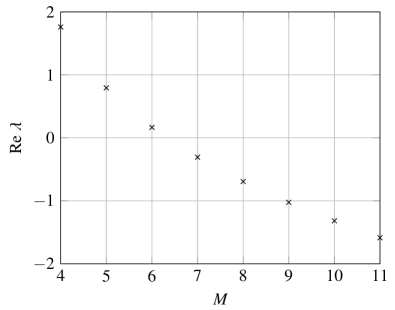
Figure 5: The real part of the dominant singularity $\operatorname{Re}\lambda_{*,0}$ as function of $M$ for the quantum wire model. It changes sign around $M=7$, so that $\lambda_{*,0}$ changes from a back-door to a front-door singularity.

If one tries to characterize $\lambda_{*,0}$ as an intruder state, it is revealed in Figure 5 that $\operatorname{Re}\lambda_{*,0}$ changes sign as $M$ is increased. This means that the characterization as “front-door” or “back-door intruders” Helgaker et al. (2002) is dependent on the basis used.

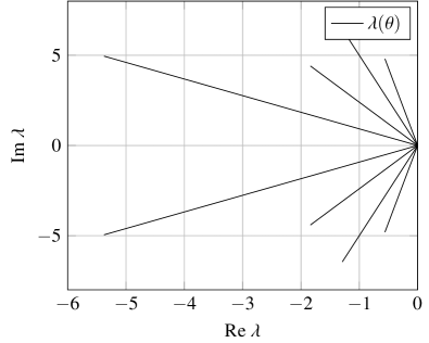
Figure 6: The smallest branch points at $M=10$ for the quantum wire model (circles) and paths $(1-\theta)\lambda_{*}$ used for determining which branches $E_{n}(\lambda)$ meet at $\lambda_{*}$. See also Figure 7.

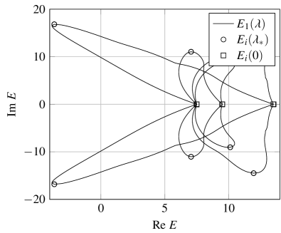
Figure 7: The eigenvalue $E_{0}(\lambda_{*})$ (squares) corresponding to the branch points $\lambda_{*}$ in Figure 6. Also shown are the paths $E_{n}[(1-\theta)\lambda_{*}]$ for the branching eigenvalues, determining which branches $E_{n}(\lambda)$ actually meet at $\lambda_{*}$.

To illustrate the continuation procedure for determining which eigenvalues branch a given $\lambda_{*}$, we have shown a number of the branch points involving the ground state $E_{0}(\lambda)$ and some other $E_{n}(\lambda)$ in Figure 6. We construct a path $\lambda(\theta)=(1-\theta)\lambda_{*}$ (also shown) and compute the eigenvalues of $H(\lambda(\theta))$ that branch at $\lambda_{*}$. As these are continued to $\lambda(1)=0$, they will be equal to unperturbed energies, and the branches are easy to determine. In Fig. 7 the eigenvalue paths $E_{0}(\lambda(\theta))$ and $E_{n}(\lambda(\theta))$ are shown. It is clearly seen that the ground state and some excited state meet at $\lambda_{*}$. This also shows how the continuation procedure may be used to find the non-dominant singularities involving the ground state, which can be taken as input for approximant construction.

III.4 A helium-like model

The final example is a helium-like model in one spatial dimension, also considered by Herman and Hagedorn Herman and Hagedorn (2009). It shares many of the qualitative features with the true helium atom in three spatial dimensions, and our goal is to determine the ROC for a Møller–Plesset calculation of the ground state energy. The model has the Hamiltonian

$$\mathcal{H} = \sum_{i=1}^{2}\left(-\frac{1}{2}\frac{\partial^{2}}{\partial x_{i}^{2}}-Z\delta(x_{i})\right)+\delta(x_{1}-x_{2})$$

$$= \mathcal{H}_{0}+\mathcal{V},$$

where $\mathcal{V}=\delta(x_{1}-x_{2})$ is the inter-electron interaction. The two electrons also interact with the nucleus of charge $Z$ via $\delta$-function potentials. We set $Z=1.38$ for the calculations.

For Møller–Plesset perturbation theory we rewrite the physical Hamiltonian as

$$\mathcal{H}=\mathcal{H}_{0}+\mathcal{U}^{\text{HF}}+(\mathcal{V}-\mathcal{U}^{\text{HF}}),$$ (6)

where the Hartree–Fock operator $\mathcal{U}^{\text{HF}}$ is defined in the usual way Helgaker et al. (2002). Since we are going to treat $\mathcal{V}-\mathcal{U}^{\text{HF}}$ as a perturbation, we introduce a parameter $\lambda$, viz,

$$\mathcal{H}^{\text{HF}}(\lambda)=\mathcal{H}_{0}+\mathcal{U}^{\text{HF}}+\lambda(\mathcal{V}-\mathcal{U}^{\text{HF}}).$$

for which $\mathcal{H}^{\text{HF}}(1)=\mathcal{H}$. We now wish to determine whether the MP series converges, i.e., the radius of convergence must be greater than $R=1$.

For this, we need to determine the Hartree–Fock basis and energies. We do this using a linear finite element basis over the interval $[-L,L]$ using $n$ sub-intervals of length $\Delta x=2L/n$ to obtain the usual Roothan–Hall equations which are solved iteratively Helgaker et al. (2002). In our calculations we have $L=15$ and $n=1000$, giving $\Delta x=0.03$. The exact solution to the Hartree–Fock ground state can be obtained in this case Herman and Hagedorn (2009) which provides a good check on the accuracy of the implementation.

The discretization parameters are $\Delta x$, $L$ and the number of single-particle functions $M$ we use in the MP series. However, we will consider the spatial discretization parameters to be fixed and sufficient for an “exact” treatment of the one-body Hamiltonians, and instead only focus on $M$.

The ground state is a singlet state, for which the spatial wave function is symmetric with respect to interchange of $x_{1}$ and $x_{2}$, and has positive parity, i.e.,

$$\psi(x_{1},x_{2})=\psi(x_{2},x_{1})=\psi(-x_{1},-x_{2}).$$

There are otherwise no dynamical symmetries in this problem.

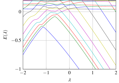
Figure 8: (Color version online) Plot of the eigenvalues $E_{n}(\lambda)$ for the helium-like model, using $M=42$ single-particle functions. Note crossing around $\lambda\approx-1.1$ with small imaginary part. We therefore expect interesting crossings with $E_{1}$ and some other $E_{n}$ to have significant imaginary part since no other avoided crossings involving the ground state is visible.

Figure 8 shows a parameter sweep of the eigenvalues of $\mathcal{H}^{\text{HF}}(\lambda)$. In this case, it is clear that there is a back-door intruder around $\operatorname{Re}\lambda_{*}\approx-1.1$, so $R\lesssim 1.1$ is obvious. It is highly likely that it corresponds to a $\beta$ type singularity in the exact problem, as there are clearly several close crossings (verified in our computations) with continuum states (with positive energy at $\lambda=0$) near $\lambda_{*}$. This is also supported by Herman and Hagedorn Herman and Hagedorn (2009).

However, it is not clear whether or not there are other branch points with, say, a small real part and imaginary part $\operatorname{Im}\lambda_{*}=0.7$, which would imply $R<1$ and hence an ultimate divergence of the MP series.

The position or existence $\beta$ singularities in the discrete problem is highly dependent on the basis chosen Olsen et al. (1996); Sergeev et al. (2005), so our conclusions must be taken relative to our discretization, which does include “diffuse” basis functions approximating the continuous spectrum.

Figure 9: Convergence radius of the helium-like model as function of the number of single-particle functions $M$. A rapid convergence towards $R\gtrsim 1.13$ is seen.

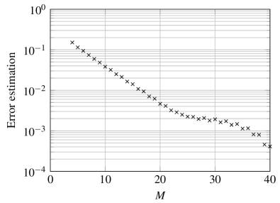
Figure 10: Estimated error in the ROC for the helium-like model as function of the number of single-particle functions $M$. An exponential error is observed, i.e., $|R(M)-R(\infty)|\sim\exp(-\beta M)$.

We compute, like in the preceding numerical examples, the dominant branch point $\lambda_{*,0}$ for various $M$ and study its behavior. For $M\leq 13$ we used the Arnoldi method, while for $M>13$ the inverse iteration method. It turns out that, in fact, $R>1$; the avoided crossing does indeed come from the dominant branch point. In Figure 9 the ROC as function of $M$ is shown. Clearly, it stabilizes around some value $R\gtrsim 1.12$. In Figure 10 an error estimate is plotted, based on the largest $M=42$, and clearly the error behaves like $\exp(-\beta M)$ where $\beta>0$ is a constant.

In Figure 11 the paths $E_{0}(\lambda(\theta))$ and $E_{1}(\lambda(\theta))$ are shown, where $\lambda(\theta)=(1-\theta)\lambda_{*,0}$. This corresponds to Figure 7 for the quantum wire model. The path is surprisingly complicated, showing that the eigenvalues may take complicated deviations from their initial unperturbed values as $\lambda$ varies in a straight line.

Figure 11: Eigenvalue path for $M=42$ for the dominant branch point $\lambda_{*,0}$. As $\lambda$ takes values along the path $(1-\theta)\lambda_{*}$, the branching eigenvalues start at $E_{n}(\lambda_{*})=E_{n^{\prime}}(\lambda_{*})$ and moves to $E_{n}(0)$ and $E_{n^{\prime}}(0)$, so that which branches meet can be determined. Here, $n=0$ and $n^{\prime}=1$.

IV Conclusion

We have described a numerical procedure to determine the singularities of the eigenvalues $E_{n}(\lambda)$ of $H_{0}+\lambda V$. Using a continuation technique that tracks eigenvalues as function of $\lambda$, the dominant singularity can be found. A simple generalization of this will enable the classification of other singularities with respect to which eigenvalues branch at $\lambda_{*}$. By continuing Step 2 and Step 3 in Algorithm 3 after $\lambda_{*,0}$ has been found, one can find the secondary dominating branch point and so on.

The method has been successfully applied to instructive examples, and in particular the convergence of a Møller–Plesset perturbation series for a helium-like model was established.

The most important virtue of the method is that it searches the whole complex plane for singularities, and also in principle can find all these. This allows a much more detailed mapping of the singularity structure than the standard methods based on the asymptotic form of the terms in the series.

Computing the singularities of $E_{n}(\lambda)$ is much harder than computing only $E_{n}(\lambda_{\text{phys}})$. One cannot hope to be able to compute the whole set of singularities for a very large many-body system. However, obtaining insight into the distribution of singularities for “typical” quantum systems, such as the examples considered in this paper and others Sergeev et al. (2005), makes the construction and analysis of general resummation schemes easier Katz (1962); Goodson (2003). Considering that popular approaches to the many-body problem such as coupled cluster methods can be viewed in terms of perturbation series only serves to emphasize the importance of calculations of singularity structures.

References

- Christiansen et al. (1996) O. Christiansen, J. Olsen, P. Jørgensen, H. Koch, and P.-Å. Malmqvist, Chem. Phys. Lett. 261, 369 (1996), ISSN 0009-2614.
- Olsen et al. (1996) J. Olsen, O. Christiansen, H. Koch, and P. Jørgensen, J. Chem. Phys. 105, 5082 (1996).
- Dunning Jr. and Peterson (1998) T. H. Dunning Jr. and K. A. Peterson, J. Chem. Phys. 108, 4761 (1998).
- Stillinger (2000) F. H. Stillinger, J. Chem. Phys. 112, 9711 (2000).
- Leininger et al. (2000) M. L. Leininger, W. D. Allen, H. F. Schaefer III, and C. D. Sherrill, J. Chem. Phys. 112, 9213 (2000).
- Roth and Langhammer (2010) R. Roth and J. Langhammer, Phys. Lett. B 683, 272 (2010), ISSN 0370-2693.
- Bartlett (1981) R. J. Bartlett, Ann. Rev. Phys. Chem. 32, 359 (1981).
- Brändas and Goscinski (1970) E. Brändas and O. Goscinski, Phys. Rev. A 1, 552 (1970).
- Goodson (2000) D. Z. Goodson, J. Chem. Phys. 112, 4901 (2000).
- Goodson (2003) D. Z. Goodson, Int. J. Quant. Chem. 92, 35 (2003), ISSN 1097-461X.
- Sergeev and Goodson (2006) A. V. Sergeev and D. Z. Goodson, J. Chem. Phys. 124, 094111 (pages 11) (2006).
- Siu et al. (2009) L.-W. Siu, J. W. Holt, T. T. S. Kuo, and G. E. Brown, Phys. Rev. C 79, 054004 (2009).
- Hunter and Guerrieri (1980) C. Hunter and B. Guerrieri, SIAM J. Appl. Math. 39, 248 (1980).
- Pearce (1978) C. J. Pearce, Adv. Phys. 27, 89 (1978).
- Zamastil and Vinette (2005) J. Zamastil and F. Vinette, J. Phys. A: Math. Gen. 38, 4009 (2005).
- Helgaker et al. (2002) T. Helgaker, P. Jørgensen, and J. Olsen, Molecular Electronic-Structure Theory (Wiley, 2002).
- Sergeev et al. (2005) A. V. Sergeev, D. Z. Goodson, S. E. Wheeler, and W. D. Allen, J. Chem. Phys. 123, 064105 (pages 11) (2005).
- Herman and Hagedorn (2009) M. Herman and G. Hagedorn, Int. J. Quant. Chem. 109, 210 (2009).
- Laidig et al. (1985) W. D. Laidig, G. Fitzgerald, and R. J. Bartlett, Chem. Phys. Lett. 113, 151 (1985), ISSN 0009-2614.
- Handy et al. (1985) N. C. Handy, P. J. Knowles, and K. Somasundram, Theor. Chim. Acta 68, 87 (1985), ISSN 1432-881X, 10.1007/BF00698753.
- Patil (2006) S. Patil, Eur. J. Phys. 27, 899 (2006).
- Reimann and Manninen (2002) S. M. Reimann and M. Manninen, Rev. Mod. Phys 74, 1283 (2002).
- Kato (1995) T. Kato, Perturbation theory for linear operators (Springer, 1995).
- Schucan and Weidenmüller (1973) T. H. Schucan and H. A. Weidenmüller, Ann. Phys. 76, 483 (1973).
- Jarlebring et al. (2010) E. Jarlebring, S. Kvaal, and W. Michiels, TW Report 559, Department of Computer Science, Katholieke Universiteit Leuven, Belgium (2010), submitted, URL http://www.cs.kuleuven.be/publicaties/rapporten/tw/TW559.pdf.
- Katz (1962) A. Katz, Nucl. Phys. 29, 353 (1962).
- Baker (1971) G. A. Baker, Rev. Mod. Phys. 43, 479 (1971).
- Goodson and Sergeev (2004) D. Z. Goodson and A. V. Sergeev, Adv. Chem. Phys. 47, 193 (2004).
- Saad (1992) Y. Saad, Numerical Methods for Large Eigenvalue Problems (Manchester University Press, 1992).
- Bartels and Stewart (1972) R. Bartels and G. Stewart, Communications of the ACM 15, 820 (1972).
- Krantz (1999) S. G. Krantz, Handbook of Complex Variables (Birkhäuser, 1999).
- Seydel (2010) R. Seydel, Practical bifurcation and stability analysis, vol. 5 (Springer, 2010), 3rd ed.