Properties of highly frustrated magnetic molecules studied by the finite-temperature Lanczos method

Abstract

The very interesting magnetic properties of frustrated magnetic molecules are often hardly accessible due to the prohibitive size of the related Hilbert spaces. The finite-temperature Lanczos method is able to treat spin systems for Hilbert space sizes up to $10^{9}$. Here we first demonstrate for exactly solvable systems that the method is indeed accurate. Then we discuss the thermal properties of one of the biggest magnetic molecules synthesized to date, the icosidodecahedron with antiferromagnetically coupled spins of $s=1/2$. We show how genuine quantum features such as the magnetization plateau behave as a function of temperature.

1 Introduction

The magnetism of antiferromagnetically coupled and geometrically frustrated magnetic molecules BGG:JCSDT97 ; MSS:ACIE99 ; SHS:PRL02 ; MTS:AC05 ; SNS:PRL05 ; TEM:CEJ06 ; SRC:PRB06 ; TMB:ACIE07 ; PLK:CC07 is a fascinating subject due to the richness of phenomena that are observed Ram:ARMS94 ; Gre:JMC01 as well as due to the similarities that can be drawn towards extended spin systems such as the two-dimensional kagomé lattice SHS:PRL02 ; Gre:JMC01 ; Diep94 ; NKH:EPL04 ; Zhi:PRL02 ; Atw:NM02 . But although molecules constitute finite-size spin systems, the investigation of their magnetic properties for instance in the Heisenberg model – as function of both temperature and magnetic field – is largely restricted if not impossible due to the enormous size of the underlying Hilbert spaces. Quantum Monte Carlo (QMC) calculations are of no help in this case since they suffer from the so-called negative-sign problem SaK:PRB91 ; San:PRB99 ; EnL:PRB06 . Density Matrix Renormalization Group (DMRG) techniques provide another very powerful approximation mainly for one-dimensional spin systems such as chains Whi:PRB93 ; Sch:RMP05 . The method delivers the relative ground states for orthogonal subspaces. Extensions to include the approximate evaluation of excitations have been developed recently Jec:PRB02 . Nevertheless, the whole method still works best for one-dimensional systems; applications to magnetic molecules are rare ExS:PRB03 .

A method, which can treat medium size spin systems irrespective of their geometric structure, is the Lanczos method Lan:JRNBS50 . This method yields eigenstates with extremal eigenvalues in orthogonal subspaces with high accuracy and is thus able to deliver a magnetization curve at $T=0$. An extension towards $T>0$ is the finite-temperature Lanczos method (FTLM) PhysRevB.49.5065 . Although it was applied to several Heisenberg or Hubbard model systems, see e.g. PhysRevB.49.5065 ; JaP:AP00 ; PhysRevB.67.161103 ; ZST:PRB06 ; PhysRevB.76.125113 ; PhysRevB.79.115141 , one must say, that this method is not yet very common.

In this article we investigate whether the finite-temperature Lanczos method (FTLM) is applicable for the Heisenberg model describing magnetic molecules. To this end its accuracy is first compared for exactly solvable cases. Thanks to recent advances in the application of group theoretical methods, the energy spectra of spin systems of unprecedented size can be evaluated numerically exactly ScS:IRPC10 . Thus, antiferromagnetically coupled spin systems with the geometric structure of the cuboctahedron and the icosahedron with $s=3/2$ will serve as test cases; the Hilbert space dimension is 16,777,216 for both ScS:IRPC10 ; ScS:PRB09 ; ScS:P09 .

Finally, the finite temperature behavior of an antiferromagnetically coupled spin system with the geometric structure of the icosidodecahedron, that is closely related to the kagomé lattice, will be examined for $s=1/2$ for the first time. Although its total Hilbert space dimension is 1,073,741,824, the finite-temperature Lanczos method is able to deliver the magnetization and the heat capacity as function of both temperature and applied magnetic field.

The article is organized as follows. In Section 2 basics of the finite-temperature Lanczos method are repeated. Section 3 is devoted to the discussion of the accuracy of the method, and in Section 4 the method is applied to the icosidodecahedron. The article closes with a summary.

2 Reminder of the finite-temperature Lanczos method

For the evaluation of thermodynamic properties in the canonical ensemble the exact partition function $Z$ depending on temperature $T$ and magnetic field $B$ is given by

$$Z(T,B) = \sum_{\nu}\;\langle\,{\nu}\,|\,e^{-\beta\!\hbox{}\mathop{\vphantom{H}\smash{H}}\limits_{\sim}\hbox{}\!}\,|\,{\nu}\,\rangle\ .$$ (1)

Here $\{\,|\,{\nu}\,\rangle\}$ denotes an orthonormal basis of the respective Hilbert space. Following the ideas of Refs. PhysRevB.49.5065 ; JaP:AP00 the unknown matrix elements are approximated as

$$\langle\,{\nu}\,|\,e^{-\beta\!\hbox{}\mathop{\vphantom{H}\smash{H}}\limits_{\sim}\hbox{}\!}\,|\,{\nu}\,\rangle \approx \sum_{n=1}^{N_{L}}\;\langle\,{\nu}\,|\,{n(\nu)}\,\rangle e^{-\beta\epsilon_{n}^{(\nu)}}\langle\,{n(\nu)}\,|\,{\nu}\,\rangle\ ,$$ (2)

where $\,|\,{n(\nu)}\,\rangle$ is the $n$-th Lanczos eigenvector starting from $\,|\,{\nu}\,\rangle$ as the initial vector of a Lanczos iteration. $\epsilon_{n}^{(\nu)}$ denotes the associated $n$-th Lanczos energy eigenvalue. The number of Lanczos steps is chosen as $N_{L}$. In addition, the complete and thus very large sum over all states $\,|\,{\nu}\,\rangle$ is replaced by a summation over a subset of $R$ random vectors. Altogether this yields for the partition function

$$Z(T,B) \approx \frac{\text{dim}({\mathcal{H}})}{R}\sum_{\nu=1}^{R}\;\sum_{n=1}^{N_{L}}\;e^{-\beta\epsilon_{n}^{(\nu)}}|\langle\,{n(\nu)}\,|\,{\nu}\,\rangle|^{2}\ .$$ (3)

Although this already sketches the general idea, it will always improve the accuracy if symmetries are taken into account as in the following formulation

$$Z(T,B) \approx \sum_{\Gamma}\;\frac{\text{dim}({\mathcal{H}}(\Gamma))}{R_{\Gamma}}\sum_{\nu=1}^{R_{\Gamma}}\;\sum_{n=1}^{N_{L}}\;$$ (4)

$$\times e^{-\beta\epsilon_{n}^{(\nu,\Gamma)}}|\langle\,{n(\nu,\Gamma)}\,|\,{\nu,\Gamma}\,\rangle|^{2}\ .$$

Here $\Gamma$ labels the irreducible representations of the employed symmetry group. The full Hilbert space is decomposed into mutually orthogonal subspaces ${\mathcal{H}}(\Gamma)$.

An observable would then be calculated as

$$O(T,B) \approx \frac{1}{Z(T,B)}\sum_{\Gamma}\;\frac{\text{dim}({\mathcal{H}}(\Gamma))}{R_{\Gamma}}\sum_{\nu=1}^{R_{\Gamma}}\;\sum_{n=1}^{N_{L}}\;e^{-\beta\epsilon_{n}^{(\nu,\Gamma)}}$$ (5)

$$\times\langle\,{n(\nu,\Gamma)}\,|\,\!\hbox{}\mathop{\vphantom{O}\smash{O}}\limits_{\sim}\hbox{}\!\,|\,{\nu,\Gamma}\,\rangle\langle\,{\nu,\Gamma}\,|\,{n(\nu,\Gamma)}\,\rangle\ .$$

It was noted in Ref. PhysRevB.67.161103 that this approximation of the observable $O(T,B)$ may contain large statistical fluctuations at low temperatures due to the randomness of the set of states $\{\,|\,{\nu,\Gamma}\,\rangle\}$. It was shown that this can largely be cured by assuming a symmetrized version of Eq. (5). For our investigations this is irrelevant.

The very positive experience is that even for large problems the number of random starting vectors as well as the number of Lanczos steps can be chosen rather small, e.g. $R\approx 20,N_{L}\approx 100$. The later sections will provide further evidence for this statement.

It is foreseeable that the method does not work optimally in very small subspaces or subspaces with large degeneracies of energy levels especially if the symmetry is not broken up into irreducible representations $\Gamma$. The underlying reason is given by the properties of the Lanczos method itself that fails to dissolve such degeneracies. The other case of small subspaces can be solved by including their energy eigenvalues and eigenstates exactly.

Another technical issue is given by the fact that the chosen random vectors $\,|\,{\nu,\Gamma}\,\rangle$ should be mutually orthogonal. Although one could orthonormalize the respective vectors, this is for practical purposes not really necessary. The reason is, that two vectors with random components are practically always orthogonal, because their scalar product is a sum over fluctuating terms that nearly vanishes especially in very large Hilbert spaces.

Since Lanczos iterations consist of matrix vector multiplications they can be parallelized by

penMP
directives. In 

ur programs this is further accelerated by an analytical state coding and an evaluation of matrix elements of the Heisenberg Hamiltonian “on the fly” SHS:JCP07 .

3 Cuboctahedron and Icosahedron

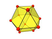
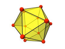
Figure 1: Structure of the cuboctahedron (left) and the icosahedron (right). The bullets represent spin sites, the edges indicate interactions.

Before employing an approximation it is necessary to estimate its accuracy by comparing to known exact results. For this purpose we choose two highly frustrated model systems that have been treated numerically exactly ScS:IRPC10 ; ScS:PRB09 ; ScS:P09 ; ScS:IRPC10 . In both systems, the cuboctahedron and the icosahedron (Fig. 1), the spins are supposed to be mounted on the vertices of the body. All spins interact antiferromagnetically with their nearest neighbors, i.e. along the edges of the body. The complete Hamiltonian of the spin system is given by the Heisenberg and the Zeeman term, i. e.

$$\!\hbox{}\mathop{\vphantom{H}\smash{H}}\limits_{\sim}\hbox{}\! = -2\;\sum_{i<j}\;{J}_{ij}\!\hbox{}\mathop{\vphantom{\vec{s}}\smash{\vec{s}}}\limits_{\sim}\!{}_{i}\cdot\!\hbox{}\mathop{\vphantom{\vec{s}}\smash{\vec{s}}}\limits_{\sim}\!{}_{j}+g\,\mu_{B}\,B\,\sum_{i}\;\!\hbox{}\mathop{\vphantom{s}\smash{s}}\limits_{\sim}\!{}^{z}_{i}\ .$$ (6)

${J}_{ij}$ is the exchange parameter between spins at sites $i$ and $j$. The antiferromagnetic case discussed in this article corresponds to negative ${J}_{ij}$. For the sake of simplicity it is assumed that all spins have the same spin quantum number $s_{1}=s_{2}=\dots=s_{N}=s=3/2$ as well as the same $g$-factor, and that ${J}_{ij}=J$ for nearest neighbors and zero otherwise.

$M$	$\text{dim}({\mathcal{H}}(M))$	$R_{1}$	$R_{2}$	$R_{3}$	$R_{4}$
18	1	exact	exact	exact	exact
17	12	exact	exact	exact	exact
16	78	exact	exact	exact	exact
15	364	exact	exact	exact	exact
14	1353	exact	exact	exact	exact
13	4224	exact	exact	exact	exact
12	11440	exact	exact	exact	exact
11	27456	1	5	20	100
10	59268	1	5	20	100
9	116336	1	5	20	100
8	209352	1	5	20	100
7	347568	1	5	20	100
6	534964	1	5	20	100
5	766272	1	5	20	100
4	1024464	1	5	20	100
3	1281280	1	5	20	100
2	1501566	1	5	20	100
1	1650792	1	5	20	100
0	1703636	1	5	20	100

Table 1: Employed number $R_{i}$ of random starting states for the cuboctahedron as well as the icosahedron with $s=3/2$: the columns provide the magnetic quantum number $M$, the dimensions of the subspaces ${\mathcal{H}}(M)$, and the $R_{i}$. “exact” means that this subspace is included completely and exactly. The data for negative $M$ are given by the symmetry $M\leftrightarrow-M$.

Since $\left[\!\hbox{}\mathop{\vphantom{H}\smash{H}}\limits_{\sim}\hbox{}\!,\!\hbox{}\mathop{\vphantom{{S}}\smash{{S}}}\limits_{\sim}\!{}^{z}\right]=0$, this (simple) symmetry is used for the finite-temperature Lanczos calculations. Table 1 shows, how the complete Hilbert space is decomposed into subspaces ${\mathcal{H}}(M)$ with total magnetic quantum number $M$. Besides the dimensions of those subspaces the table also lists four scenarios $R_{1}$, $R_{2}$, $R_{3}$, and $R_{4}$, that are used for the realization of the FTLM. As mentioned earlier, small subspaces, here with $M\geq 12$, are treated exactly.

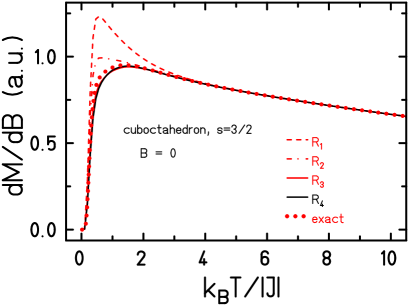
Figure 2: Zero-field differential susceptibility of the cuboctahedron with $s=3/2$. The various curves depict the investigated scenarios $R_{i}$; $N_{L}=100$. The exact dependence is given by the dots.

Figure 2 displays the zero-field differential susceptibility of the cuboctahedron with $s=3/2$. One notices that the approximate result, that anyway deviates from the exact one only for $0.5\leq k_{B}T/|J|\leq 3$, quickly approaches the exact curve with increasing number $R$ of initial states. Already for $R=20$ the approximation is practically indistinguishable from the exact one; an increase to $R=100$ does not further improve this observable.

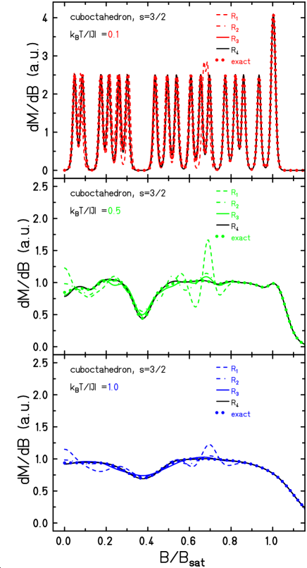
Figure 3: Differential susceptibility of the cuboctahedron with $s=3/2$ for three temperatures. The various curves depict the investigated scenarios $R_{i}$; $N_{L}=100$. The exact dependence is given by the dots.

Figure 3 shows the same observable, but this time as a function of the applied field for three low temperatures. Here one clearly observes that $R_{1}=1$ leads to large deviations at various fields. For $R_{2}=5$ the deviations are smaller but still too big for a good approximation. The approximations for $R_{3}=20$ and $R_{4}=100$ are again very good for the very low temperature of $k_{B}T/|J|=0.1$ which is due to the fact that low-lying levels which are dominant at this temperature are well approximated with $N_{L}=100$ Lanczos steps. But for temperatures of the order of the exchange interaction deviations can be observed around the minimum at $B=B_{\text{sat}}/3$ for $R_{3}=20$. This minimum is related to the magnetization plateau with $M=M_{\text{sat}}/3$, see Refs.  SSR:JMMM05 ; RLM:PRB08 ; Moe:JPCS09 ; Sch:DT10 . It seems that for smaller $R$ the higher-lying density of states is not quite accurately reproduced in subspaces around $M=M_{\text{sat}}/3$.

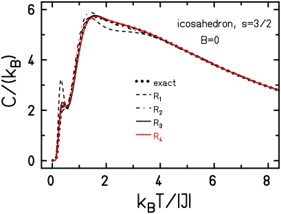
Figure 4: Zero-field heat capacity of the icosahedron with $s=3/2$. The various curves depict the investigated scenarios $R_{i}$; $N_{L}=100$. The exact dependence is given by the dots.

The magnetic properties of the icosahedron with spin $s=3/2$ are discussed in Ref. ScS:IRPC10 . Analogous to the cuboctahedron its Heisenberg Hamiltonian can be diagonalized numerically exactly with the help of point group symmetries. Here we would like to compare the exact zero-field heat capacity with the results of the finite-temperature Lanczos method, again for the scenarios listed in Table 1. The reason to choose the heat capacity and not the susceptibility is given by the fact that the heat capacity has an unusual feature at $k_{B}T/|J|\approx 0.5$ which can be described as a small low-temperature Schottky peak. It stems from a bunch of low-lying degenerate and nearly degenerate energy levels ScS:IRPC10 . In addition the main maximum has a rather unusual shape compared to other magnetic molecules where the main maximum is sharper and as a function of temperature drops off much more quickly towards the $1/T^{2}$ behavior at high temperatures.

As one can see in Fig. 4 an approximation with just one starting state ($R_{1}=1$) for each subspace is neither able to reproduce the Schottky peak nor the main maximum. This is already much better for $R_{2}=5$ and practically almost perfect for $R_{3}=20$. We would like to emphasize once more that this result is achieved with a very small number of states. As Table 1 shows, the low-$M$ subspaces assume a size of about 1.5 millions whereas the FTLM generates only $R\cdot N_{L}$ states in these subspaces, which for $R_{3}=20$ corresponds to just 2,000 states. The calculations with $R_{4}=100$ practically coincide with those for $R_{3}=20$; for the little Schottky peak the accuracy is even further improved.

4 Icosidodecahedron

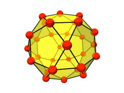
Figure 5: Structure of the icosidodecahedron. The bullets represent the 30 spin sites, the edges indicate the 60 exchange interactions. The structure is also termed Keplerate.

The icosidodecahedron of antiferromagnetically coupled spins is a very fascinating object, see Fig. 5 for the structure. Chemically it is realized with spins $s=5/2$ (abbr. Fe₃₀ MSS:ACIE99 ), $s=3/2$ (abbr. Cr₃₀ TMB:ACIE07 ), and $s=1/2$ (abbr. V₃₀ MTS:AC05 ; BKH:CC05 ). It belongs to the class of geometrically frustrated kagomé-like spin systems. Due to this close relation the icosidodecahedron once was termed “The kagomé on a sphere” RLM:PRB08 . These molecular structures exhibit genuine properties of antiferromagnetic spin systems built of corner sharing triangles as there are: many singlet states below the first triplet state, a pronounced magnetization plateau with $M/M_{\text{sat}}=1/3$, and a large magnetization jump to saturation SSR:EPJB01 ; SHS:PRL02 ; SSR:JMMM05 ; RLM:PRB08 ; Sch:DT10 .

$M$	$\text{dim}({\mathcal{H}}(M))$	$R_{1}$	$R_{2}$	$R_{3}$
15	1	exact	exact	exact
14	30	exact	exact	exact
13	435	exact	exact	exact
12	4060	exact	exact	exact
11	27405	exact	exact	exact
10	142506	exact	exact	exact
9	593775	10	10	20
8	2035800	2	5	20
7	5852925	2	5	20
6	14307150	1	5	20
5	30045015	1	5	20
4	54627300	1	5	20
3	86493225	1	5	20
2	119759850	1	5	20
1	145422675	1	5	20
0	155117520	1	5	20

Table 2: Employed number $R_{i}$ of random starting states for the icosidodecahedron with $s=1/2$: the columns provide the magnetic quantum number $M$, the dimensions of the subspaces ${\mathcal{H}}(M)$, and the $R_{i}$. “exact” means that this subspace is included completely and exactly.

Although these $(T=0)$ properties are accessible by means of Lanczos diagonalization in the case of $s=1/2$ SSR:JMMM05 ; RLM:PRB08 and by means of DMRG calculations for $s=3/2$ and $s=5/2$ ExS:PRB03 , the evaluation of the thermal behavior, i.e. for $T>0$, seemed to be impossible due to the prohibitive size of the Hilbert spaces. But at least for the icosidodecahedron with $s=1/2$ the finite-temperature Lanczos method could be able to deliver the temperature dependence of the magnetic observables. Table 2 lists the parameters used in our FTLM calculations. As can be deduced from the large dimensions of the subspaces ${\mathcal{H}}(M)$ such calculations are demanding. We employed the SGI Altix 4700 at the German Leibniz Supercomputing Center using openMP parallelization with up to 510 cores as well as our local BULL/ScaleMP computer with 128 cores. To provide an estimate, a run in the subspace with $M=0$ and $R_{3}=20$ together with $N_{L}=100$ needs about a full day on 510 ITANIUM II cores.

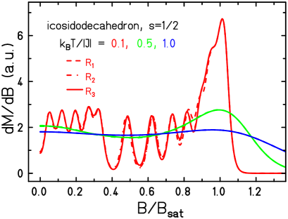
Figure 6: Differential susceptibility of the icosidodecahedron with $s=1/2$ for three temperatures. The various curves depict the investigated scenarios $R_{i}$; $N_{L}=100$.

Figure 6 compares the results of FTLM calculations with three different sets of random starting states, see Table 2. It is astonishing how little the observable varies with $R_{i}$. This means that the finite-temperature Lanczos method replaces the true spectrum very effectively by pseudo energy eigenvalues so that gross properties are efficiently reproduced.

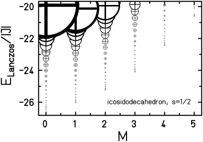
Figure 7: Top: Pseudo energy eigenvalues of the icosidodecahedron with $s=1/2$ for $R_{1}=1$ and $N_{L}=100$. Bottom: Low-energy part of the same energy spectrum, but now the size of the symbols represents the weight of the corresponding state.

It is important to note that the pseudo energy eigenvalues, see top of Fig. 7, have no spectroscopic meaning in general. Very low-lying energy levels may nearly coincide with the true ones due to the rapid convergence of the Lanczos method for extremal eigenvalues. The vast majority of levels – together with their weights(!) – has to be understood as an effective representation of the energy level density. To make this point clearer the bottom of Fig. 7 displays the low-energy part of the spectrum with symbols whose radii represent the weights with which they have to be multiplied to the Boltzmann factor in the partition function. In effect the method has some similarities with the classical Wang-Landau sampling WaL:PRL01 ; WaL:PRE01 ; ZST:PRL06 , where one also constructs an approximate density of states consisting of discretized energy intervals and their weights in order to later evaluate thermal properties SBL:PRB07 .

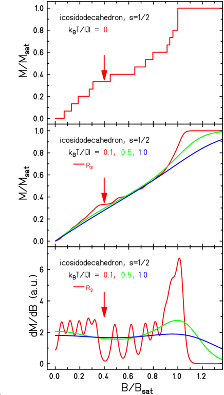
Figure 8: Top and middle: Magnetization of the icosidodecahedron with $s=1/2$ for four temperatures and $R_{3}=20$; $N_{L}=100$. The plateau with $M/M_{\text{sat}}=1/3$ is indicated by an arrow. The other steps of the magnetization curve are due to the finite size of the spin system. Bottom: corresponding differential susceptibility; here the plateau expresses itself as a dip.

The successful determination of the temperature dependence enables us to discuss several thermal properties of the icosidodecahedron with $s=1/2$. A key question is the width and thermal evolution of the magnetization plateau with $M/M_{\text{sat}}=1/3$. This plateau expresses itself in the differential susceptibility as a dip. Classical calculations for the $s=5/2$ case yielded a dip that is much narrower than the experimental findings SNS:PRL05 . It was not evident how this feature would behave in a quantum calculation. Figure 8 shows both the magnetization (top and middle) as well as the differential susceptibility (bottom). The plateau with $M/M_{\text{sat}}=1/3$ is indicated by an arrow. Interestingly, the plateau as well as the dip disappear quickly with rising temperature. Already for $k_{B}T/|J|=0.5$ they are hardly visible, and the position of the now much broader dip is shifted to higher fields. It is not yet obvious – and thus will be a matter of future research – how this trend transfers to quantum icosidodecahedra with $s=5/2$ or $s=3/2$ and whether it would be sufficient to explain the experimental findings SPK:PRB08 .

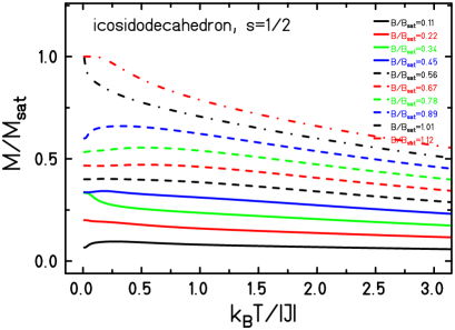
Figure 9: Magnetization of the icosidodecahedron with $s=1/2$ for various magnetic field strengths and $R_{3}=20$; $N_{L}=100$.

Another feature, that was observed for the icosidodecahedron with $s=5/2$, is the near constancy of the magnetization as a function of temperature for some magnetic fields SLM:EPL01 . Figure 9 displays the theoretical magnetizations for low temperatures and several magnetic field strengths, but now of course for $s=1/2$. There are field ranges, e.g. $B/B_{\text{sat}}\approx 0.4,\dots,0.8$, where the magnetization varies indeed very little with temperature. This is also seen in the middle part of Fig. 8, where the magnetization curves for three temperatures virtually fall on top of each other in the respective field interval. At the moment it is a speculation how this behavior would change for larger spins such as $s=5/2$. One could conjecture that the field ranges of the plateau as well as of the rise to saturation might shrink relatively and thus lead to thermally stable magnetization in broader field intervals.

Figure 10: Zero-field heat capacity of the icosidodecahedron with $s=1/2$ and $R_{3}=20$; $N_{L}=100$ (solid curve). For comparison the zero-field differential susceptibility is given by a dashed curve.

Finally, we would like to discuss the heat capacity of the icosidodecahedron with $s=1/2$. Figure 10 shows the zero-field heat capacity that is obtained for $R_{3}=20$ and $N_{L}=100$. Since the system possesses many singlets below the first triplet one expects low-temperature features in the specific heat curve, that are indeed clearly visible (solid curve). They are absent in the zero-field differential susceptibility (dashed curve) that is provided for comparison. In addition the main maximum of the specific heat is at higher temperatures than that of the susceptibility which points at a higher-lying density of states that shows up in the heat capacity but has not much impact on the susceptibility.

5 Summary and Outlook

The finite-temperature Lanczos method enabled us to evaluate the thermal properties of the antiferromagnetic spin icosidodecahedron with $s=1/2$. The magnetic susceptibility as well as the heat capacity could be determined. A major result is that the magnetization plateau at $M/M_{\text{sat}}=1/3$ is thermally rather unstable, i.e. it disappears above temperatures of $k_{B}T/|J|\approx 0.5$.

An important open question is how our findings change if the spin is increased, e.g. to $s=5/2$ for the iron based icosidodecahedron. Intuitively one would guess that quantum features are decreased for the more classical spin. For the smaller but similar cuboctahedron it could be shown that the number of singlets below the first triplet state decreases with increasing spin quantum number ScS:P09 . This would have an impact on the low-temperature features of heat capacity. Further investigations are necessary to clarify such questions which are of general nature for all kagomé-like spin systems.

References

- (1) A. J. Blake et al., J. Chem. Soc. Dalton Trans. 485 (1997).
- (2) A. Müller et al., Angew. Chem. Int. Ed. 38, 3238 (1999).
- (3) J. Schulenburg et al., Phys. Rev. Lett. 88, 167207 (2002).
- (4) A. Müller et al., Angew. Chem., Int. Ed. 44, 3857 (2005).
- (5) C. Schröder et al., Phys. Rev. Lett. 94, 017205 (2005).
- (6) E. I. Tolis et al., Chem. Eur. J. 12, 8961 (2006).
- (7) J. van Slageren et al., Phys. Rev. B 73, 014422 (2006).
- (8) A. M. Todea et al., Angew. Chem. Int. Ed. 46, 6106 (2007).
- (9) C. P. Pradeep, D.-L. Long, P. Kögerler, and L. Cronin, Chem. Commun. 4254 (2007).
- (10) A. P. Ramirez, Annu. Rev. Mater. Sci. 24, 453 (1994).
- (11) J. Greedan, J. Mater. Chem. 11, 37 (2001).
- (12) Magnetic systems with competing interactions, edited by H. Diep (World Scientific, Singapore, 1994).
- (13) Y. Narumi et al., Europhys. Lett. 65, 705 (2004).
- (14) M. E. Zhitomirsky, Phys. Rev. Lett. 88, 057204 (2002).
- (15) J. L. Atwood, Nat. Mater. 1, 91 (2002).
- (16) A. W. Sandvik and J. Kurkijärvi, Phys. Rev. B 43, 5950 (1991).
- (17) A. W. Sandvik, Phys. Rev. B 59, R14157 (1999).
- (18) L. Engelhardt and M. Luban, Phys. Rev. B 73, 054430 (2006).
- (19) S. R. White, Phys. Rev. B 48, 10345 (1993).
- (20) U. Schollwöck, Rev. Mod. Phys. 77, 259 (2005).
- (21) E. Jeckelmann, Phys. Rev. B 66, 045114 (2002).
- (22) M. Exler and J. Schnack, Phys. Rev. B 67, 094440 (2003).
- (23) C. Lanczos, J. Res. Nat. Bur. Stand. 45, 255 (1950).
- (24) J. Jaklič and P. Prelovšek, Phys. Rev. B 49, 5065 (1994).
- (25) J. Jaklič and P. Prelovšek, Adv. Phys. 49, 1 (2000).
- (26) M. Aichhorn, M. Daghofer, H. G. Evertz, and W. von der Linden, Phys. Rev. B 67, 161103 (2003).
- (27) I. Zerec, B. Schmidt, and P. Thalmeier, Phys. Rev. B 73, 245108 (2006).
- (28) B. Schmidt, P. Thalmeier, and N. Shannon, Phys. Rev. B 76, 125113 (2007).
- (29) J. Almeida, M. A. Martin-Delgado, and G. Sierra, Phys. Rev. B 79, 115141 (2009).
- (30) R. Schnalle and J. Schnack, Int. Rev. Phys. Chem. 29, 403 (2010).
- (31) R. Schnalle and J. Schnack, Phys. Rev. B 79, 104419 (2009).
- (32) J. Schnack and R. Schnalle, Polyhedron 28, 1620 (2009).
- (33) J. Schnack, P. Hage, and H.-J. Schmidt, J. Comput. Phys. 227, 4512 (2008).
- (34) R. Schmidt, J. Schnack, and J. Richter, J. Magn. Magn. Mater. 295, 164 (2005).
- (35) I. Rousochatzakis, A. M. Läuchli, and F. Mila, Phys. Rev. B 77, 094420 (2008).
- (36) R. Moessner, J. Phys.: Conf. Ser. 145, 012001 (2009).
- (37) J. Schnack, Dalton Trans. 39, 4677 (2010).
- (38) B. Botar, P. Kögerler, and C. L. Hill, Chem. Commun. 3138 (2005).
- (39) J. Schnack, H.-J. Schmidt, J. Richter, and J. Schulenburg, Eur. Phys. J. B 24, 475 (2001).
- (40) F. Wang and D. P. Landau, Phys. Rev. Lett. 86, 2050 (2001).
- (41) F. Wang and D. P. Landau, Phys. Rev. E 64, 056101 (2001).
- (42) C. G. Zhou, T. C. Schulthess, S. Torbrügge, and D. P. Landau, Phys. Rev. Lett. 96, 120201 (2006).
- (43) S. Torbrügge and J. Schnack, Phys. Rev. B 75, 054403 (2007).
- (44) C. Schröder et al., Phys. Rev. B 77, 224409 (2008).
- (45) J. Schnack, M. Luban, and R. Modler, Europhys. Lett. 56, 863 (2001).