Abstract

We study some problems arising from the introduction of a complex scalar field in cosmology, modelling its possible behaviors in both the inflationary and dark energy stages of the universe. Such examples contribute to show that, while the complex nature of the scalar field can be indeed important during inflation, it loses its meaning in the later dark–energy dominated era of cosmology, when the phase of the complex field is practically constant, and there is indeed a transition from complex to real scalar field. In our considerations, the Noether symmetry approach turns out to be a useful tool once again. We arrive eventually at a potential containing the sixth and fourth powers of the scalar field, and the resulting semiclassical quantum cosmology is studied to gain a better understanding of the inflationary stage.

I Introduction

The standard treatment of an inflationary scenario, as well as of dark energy, makes use of one or more real scalar fields, variously coupled to gravity and matter. On the other hand, from the point of view of Quantum Field Theory, such scalar fields can be taken to be either real or complex. The main goal of this paper is to get a deeper understanding of the transition from complex to real scalar fields, also contributing to implement the idea that the phase of a complex field characterizing the epoch of dark energy is practically constant, so that it may be set to zero safely. We will not try here to prove this result in general form, but in particular cases of wide interest. The general proof is postponed to future studies.

On the other hand, during the inflationary epoch, the phase should very rapidly be driven to be constant, if not already, so that the assumption of real fields would turn out to be justified. We shall give an example in which this is not entirely obtained, so that further investigation of this point also seems to be necessary. Although there exists a large amount of literature concerning such kind of problems (see Refs. kasuya01 ; gu01 ; boyle02 ; wei05 ; zhao06 for example), here we want to look at things from a different point of view, adding new features and offering other examples for the discussion. Furthermore, we do not enter at all into the domain of the open question whether there exists only a scalar field (or many of them) driving both inflationary and dark energy epochs or not, since we limit ourselves just to consider the two evolutionary stages as separated.

As a matter of fact, another important feature of this work consists in the application of the Noether symmetry approach to the problem. This procedure was applied for the first time by some of us deritis90 ; capozziello96 in the context of a minimally coupled real scalar field. Since then, a lot of different results were found in various situations (as can be seen in Ref. capozziello96 , for instance, just accounting for the first results only).

Here we try to find a Noether charge, for some suitable choice of the potential ruling one single scalar field. The first interesting result is that, by virtue of the phase and of the fact that the potential depends only on the modulus, there is always a trivial symmetry and a cyclic variable (the same holds also for the hessence case). The associated charge (below called $Q$) was, on the other hand, already known (see Refs. gu01 ; boyle02 ; wei05 ; zhao06 and references therein). However, the presentation which we give here seems to us more elegant both in terms of the procedure and the interpretation, and we shall make use of this constant in order to make most of our considerations. What is more interesting is the fact that, using the Noether symmetry approach, we may prove that no other symmetry is found, except for the case $Q=0$, which indeed gives back the real case. Since we have proved elsewhere deritis90 ; capozziello96 ; rubano02 that, in the real case, a class of symmetries does exist, we see that the more fundamental picture of a complex field breaks the symmetry, which may thus be obtained only as a limiting case, when the field becomes real.

In Sec. II, we sketch the basis of our problem and find a trivial Noether charge. The following Sec. III is devoted to the possibility of determining other symmetries via the Noether symmetry approach with an exponential potential, while Sec. IV studies the equations of motion and the possibility to look at the presence of a complex scalar field as a sort of perturbation with respect to the real scalar field case, hence commenting on the numerical solution so found. This is done in the two separate situations of dark energy and inflation. Section V studies the semiclassical quantum cosmology for the scalar-field potential obtained in Sec. IV, with application to a better understanding of the conditions for inflation. Finally, in Sec. VI some conclusions are drawn.

II Setting the problem and finding a trivial charge

The observable universe and its large scale structure are usually considered to have their origins in an early inflationary stage. Driven by a single scalar field, inflation in fact yields a distribution of adiabatic density perturbations capable to give an account of what we observe today in the large scale. On the other hand, string theory or other higher-dimensional field theories consider a number of scalar fields, which could all play a role during this early stage of evolution of the universe. This has of course to be taken into account when dealing with inflation and its consequences.

Even if considering only one scalar field can be considered as a good starting point to understand the main issues of many fundamental problems, for sake of completeness in what follows we sketch something about the possibility of considering more than one scalar field. Because of the introductory type of discussion we are aiming to do, however, we then continue our treatment by using a single scalar field.

II.1 More than one scalar field for the inflationary epoch

Inflationary dynamics and the spectrum of primordial perturbations are drastically affected by considering multiple scalar fields wands08 ; bassett06 . For instance, unlike the single-field scenario, in such a case there appear also the nonadiabatic density perturbations, which could lead to detectable specific features in future observations.

Klein–Gordon and Friedmann equations with multiple (non mutually interacting) scalar fields labelled by $i$’s are written in the homogeneous and isotropic flat case as wands08

$$\ddot{\varphi}_{i}+3H\dot{\varphi}_{i}+\frac{\partial}{\partial\varphi_{i}}(\sum_{j}U_{j}) = 0\,,$$ (1)

$$3H^{2}-8\pi G\left(\sum_{i}\frac{1}{2}{\dot{\varphi}_{i}}^{2}+V\right)=0,$$ (2)

$H$ being the Hubble parameter and $U_{j}$ the potential of the $j$-th scalar field. Here, we are also assuming that the global potential energy is given by the sum of such single potentials, as

$$V\equiv\sum_{j}U_{j}\,.$$ (3)

Since the Hubble expansion is affected by the sum of all single potentials, it is thus clear that the overall field dynamics can be substantially changed in the presence of multiple scalar fields, even if the single potentials are not affected. There are, of course, different ways to consider many fields in inflation and we will not touch upon them here. See Ref. wands08 for further comments and citations to literature.

Even if there is the possibility to reduce the background dynamics to an equivalent single field with only a potential wands08 ; malik99 , it is nevertheless important to stress again that there are meaningful differences between the scenario with multiple fields and the one with a single scalar field. While the evolution in the latter case can be shown to be independent of the initial conditions, the inflationary dynamics in the former may not. But, while keeping some distinct features of a multiple field scenario, it can anyway lead to observable predictions which may not depend on the initial conditions, as in Nflation lyth99 ; kim06 .

Implementing the inflationary paradigm with many scalar fields has gained an increasing interest, since we are now facing a period of greater precision in cosmological observations, which allows the future possibility to discriminate between these various forms of inflationary stages. But, for what concerns us here, we shall return to the single field model in the following.

II.2 A single scalar field

It is easy to verify that the Friedmann and Klein–Gordon equations for a spatially flat FLRW metric and a complex scalar field $\phi$ may be derived from the following point Lagrangian

$$L=3a\dot{a}^{2}-\frac{a^{3}}{2}(\dot{\varphi}_{1}^{2}+\dot{\varphi}_{2}^{2})+a^{3}V(\varphi)\,,$$ (4)

where we have used the metric signature $(+\,-\,-\,-)$ and adopted the units in which $8\pi G=1$, while $\varphi_{1,2}$ are the real and imaginary parts of the field $\phi$ and $\varphi\equiv\sqrt{\varphi_{1}^{2}+\varphi_{2}^{2}}$ is its modulus, so that one can write $\varphi_{1}=\varphi\cos\theta$ and $\varphi_{2}=\varphi\sin\theta$.

It is important to point out that the Lagrangian is the same in absence of matter, as well as, up to a constant, in its presence in the form of dust. The difference consists only in the value of the Energy Function associated, as usual, with $L$

$$E_{L}\equiv\sum_{i}\frac{\partial L}{\partial\dot{q}_{i}}\dot{q}_{i}-L\,,$$ (5)

which of course, in our case, should not be interpreted as the physical energy. In the case of vacuum $E_{L}$ vanishes, while in the case of dust $E_{L}=const.$, a value to be related to the present amount of matter, i.e. $\Omega_{m0}$.

The following arguments will be therefore applied in the two separate cases of inflation and dark energy, with suitable specifications when necessary. As already said, in fact, we do not want to enter into the realm of the unsolved problem of a unique scalar field, describing both the primeval era and the present accelerated expansion of the universe. Any relationship between the two fields present in such different cosmological stages is taken as inessential for our discussion, and we simply limit ourselves to consider the predominance of a complex scalar field in each one of the two epochs.

For our purposes, it is much better to introduce the phase $\theta$ so that the Lagrangian becomes

$$L=3a\dot{a}^{2}-\frac{a^{3}}{2}(\dot{\varphi}^{2}+\varphi^{2}\dot{\theta}^{2})+a^{3}V(\varphi)\,,$$ (6)

and we see at once that $\theta$ is cyclic. Thus, we immediately obtain the conserved charge

$$\Sigma\equiv-a^{3}\varphi^{2}\dot{\theta}\,,$$ (7)

as expected. The minus sign is irrelevant, as $\Sigma$ will always appear in squared form, and we shall set $Q\equiv\Sigma^{2}$. It is now clear what was stated in the introduction above: $\Sigma=0$ corresponds to the real case, for which we already have a large set of interesting results deritis90 ; capozziello96 ; rubano02 .

In order to look for other symmetries, we need to make use of the charge obtained and reduce the degrees of freedom of the system. The procedure is exactly the same as in the case of a central potential in classical mechanics. First, we write the Energy Function

$$E_{L}=3a\dot{a}^{2}-\frac{a^{3}}{2}(\dot{\varphi}^{2}+\varphi^{2}\dot{\theta}^{2})-a^{3}V(\varphi)\,,$$ (8)

and substitute for $\dot{\theta}$ to obtain

$$E_{L}=3a\dot{a}^{2}-\frac{a^{3}}{2}\dot{\varphi}^{2}-\frac{Q}{2a^{3}\varphi^{2}}-a^{3}V(\varphi)\,.$$ (9)

Finally we have the reduced Lagrangian

$$L^{\prime}=3a\dot{a}^{2}-\frac{a^{3}}{2}\dot{\varphi}^{2}+a^{3}\left(\frac{Q}{2a^{6}\varphi^{2}}+V(\varphi)\right)\,.$$ (10)

It should be stressed that this expression for the Lagrangian is not the same as the one obtained by direct substitution of Eq. (2.7) into $L$ in Eq. (6). We have in fact reduced the configuration space of the problem from $3$ degrees of freedom ($\{a,\varphi,\theta\}$) to $2$ ($\{a,\varphi\}$), as usual in this approach. We also observe that the system is now “equivalent” to that of a real field, endowed with an effective potential

$$W(a,\varphi)\equiv\frac{Q}{2a^{6}\varphi^{2}}+V(\varphi)\,,$$ (11)

as already pointed out elsewhere (see Ref. zhao06 , for example). The presence of the scale factor in $W$ substantially modifies the situation, and the field is now in a sense nonminimally coupled to gravity, although in a way which is not standard. This is of course due to the fact that the new Lagrangian is not physical, but obtained as a result of a reduction procedure.

III Looking for new symmetries

Let us now apply the standard procedure of the Noether symmetry approach in order to establish nontrivial symmetries of $L^{\prime}$. We look for a vector field on the reduced configuration space, properly lifted to the tangent space abraham78 ; marmo85 ; morandi90 ; deritis90 ; capozziello96

$$X=\alpha(a,\varphi)\frac{\partial}{\partial a}+\beta(a,\varphi)\frac{\partial}{\partial\varphi}+\dot{\alpha}(a,\varphi)\frac{\partial}{\partial\dot{a}}+\dot{\beta}(a,\varphi)\frac{\partial}{\partial\dot{\varphi}}\,,$$ (12)

such that the Lie derivative $\mathcal{L}_{X}L^{\prime}$ vanishes. Here, the two functions $\alpha(a,\varphi)$ and $\beta(a,\varphi)$ are unknown. By virtue of the linear dependence of $X$ on “velocities” and the quadratic ones of $L^{\prime}$, a quadratic polynomial in $\dot{a}$, $\dot{\varphi}$ is obtained. Since it must be identically zero, a set of four equations is finally derived, i.e.

$$\alpha+2a\frac{\partial\alpha}{\partial a} = 0\,,$$ (13)

$$3\alpha+2a\frac{\partial\beta}{\partial\varphi} = 0\,,$$ (14)

$$6\frac{\partial\alpha}{\partial\varphi}-a^{2}\frac{\partial\beta}{\partial a} = 0\,,$$ (15)

$$3\alpha V(\varphi)+a\beta\frac{dV}{d\varphi} = Q\left(\frac{3\alpha}{2a^{6}\varphi^{2}}+\frac{\beta}{a^{5}\varphi^{3}}\right)\,.$$ (16)

The first three equations are identical as in Refs. deritis90 ; capozziello96 , while the last one differs because of the presence of an effective potential, by virtue of the supposed complex nature of the scalar field. Thus, proceeding along the very same lines, it is possible to find a general solution for $\alpha$ and $\beta$, which however, when inserted into the last equation, turns out to be incompatible, unless $Q=0$ (in the latter situation, of course, a specified class of potentials is found deritis90 ; capozziello96 ).

It is thus proved that, in the fully complex case, no nontrivial symmetry exists. It should be stressed that the potential has been simply viewed as a function of $\varphi\equiv\sqrt{\varphi_{1}^{2}+\varphi_{2}^{2}}$, but the same thing can be proved also while using a potential depending on $\sqrt{\varphi_{1}^{2}-\varphi_{2}^{2}}$, so covering the well known hessence case wei05 , for instance. As a matter of fact, in the latter situation one has $\varphi\equiv\sqrt{\varphi_{1}^{2}-\varphi_{2}^{2}}$, where $\varphi_{1}\equiv\varphi\cosh\theta$ and $\varphi_{2}\equiv\varphi\sinh\theta$, so that $\coth\theta={\varphi_{1}\over\varphi_{2}}$. One then obtains the same set of Eqs. (3.2)–(3.4), while Eq. (3.5) is replaced by

$$3\alpha V(\varphi)+a\beta{dV\over d\varphi}=-Q\left({9\alpha\over 2a^{6}\varphi^{2}}+{\beta\over a^{5}\varphi^{3}}\right).$$

Of course, this does not change the qualitative features of our previous results obtained from the Noether symmetry approach. In the case $Q=0$, instead, we recover the real scalar field situation, where it is well known that a class of exponential potentials does the job deritis90 ; capozziello96 . In particular, we shall now make use of the potential

$$V=V_{0}e^{-\sqrt{\frac{3}{2}}\varphi}\,,$$ (17)

finding indeed a peculiar situation rubano02 ; rubano04 .

We are in fact used to see that in Quantum Field Theory some symmetries are generally found at a more fundamental level, which are subsequently broken during the evolution. Here, on the contrary, assuming a potential of the form in Eq. (17), we see that a complex field shows initially no symmetry. Since $Q=a^{6}\varphi^{4}\dot{\theta}^{2}$, we have that, along with the growth of the scale factor with time, and provided that $\varphi$ does not contemporarily go to zero very rapidly, $\dot{\theta}$ should approach $0$. The term with the initially nonvanishing $Q$ then becomes negligible and, at least with very good approximation, the Noether symmetry is recovered, in contrast with the usual expectation.

IV Equations of motion and numerical perturbations

It is now clear that $Q$ can be regarded as a parameter, characterizing a perturbation term in $L^{\prime}$. In this way the real scalar field corresponds to the unperturbed solution, while the phase of the complex scalar field gives rise to the perturbed solution. This point of view turns out to be particularly useful once an exact solution for the real scalar field is available. This being our case, let us first write, for the reduced Lagrangian (2.10), the Euler–Lagrange equations

$$2\frac{\ddot{a}}{a}+\left(\frac{\dot{a}}{a}\right)^{2}+\frac{1}{2}\left(\dot{\varphi}^{2}+\frac{Q}{a^{6}\varphi^{2}}\right)-V(\varphi) = 0\,,$$ (18)

$$\ddot{\varphi}+3\frac{\dot{a}}{a}\dot{\varphi}+\frac{dV}{d\varphi}-\frac{Q}{a^{6}\varphi^{3}} = 0\,,$$ (19)

and the conservation of the Energy Function

$$3a\dot{a}^{2}-\frac{a^{3}}{2}\dot{\varphi}^{2}-\frac{Q}{2a^{3}\varphi^{2}}-a^{3}V(\varphi)=E_{L}\,,$$ (20)

where, as we said, $E_{L}=0$ corresponds to the vacuum case. In this case, an important consistency check is as follows. Equation (4.1), jointly with $E_{L}=0$, yields

$${\dot{H}}=-{{\dot{\varphi}}^{2}\over 2}-{Q\over 2a^{6}\varphi^{2}}$$

for the time derivative of the Hubble parameter, once that $E_{L}=0$ is used to re-express $3H^{2}$. On the other hand, $E_{L}=0$ should have vanishing time derivative (this corresponds to preservation in time of the Hamiltonian constraint), and this yields again, upon expressing $\ddot{\varphi}$ from the Klein–Gordon equation (4.2), the formula for ${\dot{H}}$ written above, since the additional contributions of ${{\dot{\varphi}}Q\over a^{6}\varphi^{3}}$ occur with opposite signs and hence cancel each other exactly.

In what follows we shall first consider, due to its brevity, the dark energy situation and then the inflationary one. This gives no problem, since one has always to remember that we have not assumed here any relationship between the two scalar fields driving the two different stages of the cosmological evolution.

IV.1 Perturbation of a dark energy solution

Let us, now, first consider an exact solution for the dark energy scenario. In the case $Q=0$, as said above, the exponential potential in Eq. (17) exhibits a Noether symmetry. This allows exact integration of equations, as shown in Refs. rubano02 ; rubano04 . It is also possible to show that the solution fits very well with the SNIa data, as well as other tests rubano02 ; rubano04 .

Following the procedure of Ref. rubano04 we find it useful to set the unit of time to the age $t_{0}$ of the universe. This greatly simplifies notations and, above all, is of great help in numerical treatments, which are necessary when we go to the perturbed system. In these units $H_{0}$ turns out to be of order $1$, and it is in fact convenient to set it exactly to $1$. Actually, this is not the best fit value, but very near, so that it can be considered appropriate for our purposes. Other choices of the integration constants lead to $a_{0}=a(t_{0}=1)=1$, and $a(0)=0$, which are quite standard. The last constant fixes the present value of the scalar field $\varphi_{0}$. In the unperturbed system, however, this is quite arbitrary, since we are not able to observe it in any way. Here, lies a problem: if, during the evolution of the unperturbed solution, one gets $\varphi=0$, the perturbing term diverges! In order to avoid this pathology, we have set $\varphi_{0}\equiv\sqrt{2/3}\log\,2$, which is not the same as in Ref. rubano04 , but appropriately shifted.

In light of all these assumptions, the solution takes the very simple form

$$a^{3}(t) = \frac{t^{2}(1+t^{2})}{2}\,,$$ (21)

$$\varphi(t) = \sqrt{\frac{2}{3}}\log(1+t^{2})\,,$$ (22)

$$H(t) = \frac{2(1+2t^{2})}{3t(1+t^{2})}\,,$$ (23)

$$V(\varphi) = 4\exp(-\sqrt{3/2}\varphi)=\frac{4}{(1+t^{2})}\,,$$ (24)

$$\Omega_{m} = \frac{(1+t^{2})}{(1+2t^{2})^{2}}\,,$$ (25)

$$\Omega_{m0} = \frac{2}{9}\approx 0.22\,,$$ (26)

where the value of $\Omega_{m0}$ obtained here is not the best fit one, by virtue of the simplified choice of $H_{0}$. It is easy to check that the equations of motion are satisfied by this solution if $Q=0$.

With our choices, at $t_{0}$ all terms in the equations are of order $1$, so that a small perturbation is obtained for $Q<<1$. Introducing this term now requires a numerical integration, which is performed starting from $t_{0}=1$ and integrating backwards. The choice of $Q$ is of course arbitrary; let us thus set $Q=10^{-4}$, for example. The plot in Fig. (1) shows a comparison between the exact solution for the scale factor $a(t)$ and the perturbed one in the case of the exponential potential above.

Figure 1: Comparison between the exact (blue colored) and the perturbed (red colored) scale factors $a(t)$ for the exponential potential given in Eq. (17), in the dark-energy regime.

It is clearly seen that the agreement is quite good for $t\gtrsim 0.3$, as may be checked also by simple computation. Before this time, something dramatic happens and a singularity is obtained for $t\approx$ $0.088$. This is of course due to the reduced value of the denominator in the perturbation term, which prevents this from being small. A computation of the redshift at the time when the discrepancy becomes visible gives $z\approx 1.0$, which is of course untenable. Lowering the value of $Q$, would clearly push the discrepancies away, possibly up to an epoch when the model is not applicable. But this is in fact what we wanted to show. This dark energy model is viable only if the perturbing term is effectively negligible. It is also clear that any unperturbed system, for which the term $a^{3}\varphi^{2}$ tends to zero in the past, will give similar results. Thus, a better exploration of this possibility is needed.

IV.2 Perturbing an inflationary solution

Let us now move to a totally different situation, that is the earlier inflationary scenario. We want to see what happens if the perturbation term is applied to an exact solution describing primeval inflation. The general exact solution for the exponential potential in Eq. (17) can be easily specified to the new situation, but, unfortunately, what is then obtained is a power-law inflation, with behavior $a(t)\propto t^{4/3}$ capozziello96 . As is well known, the spectrum of primordial perturbations for power-law inflation $a(t)\propto t^{p}$ can be computed, and the spectral index is given approximately by

$$n_{s}\approx 1-\frac{2}{p}\,,$$ (27)

so that the higher is the exponent $p$, the nearer we are to the spectral index of the Harrison–Zel’dovich spectrum har70 ; zel72 . This means that $p$ must be sufficiently large if we want to obtain $n_{s}\approx 1$, in agreement with WMAP observations.

Thus, for the purpose of describing a more realistic situation, it is necessary to give up the Noether symmetry, but we can anyway use an exact solution for the unperturbed system. It was shown long ago lucchin85 (but see also Ref. rubano02 ) that a power-law behavior can be obtained as a particular solution from the potential

$$V=V_{0}\exp\left(-\sqrt{\frac{2}{p}}\varphi\right)\,,$$ (28)

so that

$$a=t^{p}\quad;\quad\varphi=\sqrt{2p}\log\left(t\sqrt{\frac{V_{0}}{p(3p-1)}}\right)\,,$$ (29)

where we note that the value of $V_{0}$ only fixes a shift in $\varphi$, which is on the other hand important in order to avoid singularities as above.

In this new situation, we have to fix again a suitable unit of time. A natural choice is to set the beginning of inflation at $t_{{\rm in}}=1$, i.e., if we accept the usual estimate $t_{{\rm in}}=t_{Pl}$ (the Planck time), we are restoring the usual Planck units. Let us also set $p=50$, which gives a reasonable $n$, and provides, for $t_{{\rm end}}=3.5$, an acceptable e-folding number $N_{e}\approx 62$. The small interval spanned by time is then good for the numerical integration. The last constant to be fixed is $V_{0}$, which we can arbitrarily set to $1$.

It is again easy to find that, by setting $E_{L}=0$ into Eqs. (8) and (9), and inserting Eqs. (28) and (29) into them, they are in fact verified. Now, in order to introduce the perturbation, it is necessary to establish for which value of $Q$ it turns out to be sufficiently “small”. A check of the terms in the equations at the initial point $t_{{\rm in}}$ shows that now they are far from being of order $1$. For instance, the modified Klein–Gordon equation gives at the initial point $\ddot{\varphi}=-10-0.0000112871Q$. This means that a value of, say, $Q=10^{5}$ provides a small, but not entirely negligible, perturbation.

On performing a numerical integration from $t_{{\rm in}}=1$ to $t_{{\rm end}}=3.5$ and plotting the percentage difference $\Delta$ between the exact and perturbed solutions with respect to time $t$, we obtain what is plotted in Fig. (2).

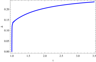
Figure 2: Plot of the percentage difference $\Delta(t)$ between the exact and perturbed solutions for the exponential potential in the inflationary regime.

This shows that such percentage difference is growing, even if slowly, up to $0.2\%$. This is clearly small, but we have to remember that we started from a small perturbation. As a matter of fact, taking a larger value like $Q=10^{7}$ allows the difference to grow up to about $15\%$.

On the basis of this result we might conclude that the treatment of inflation by means of a real scalar field would be a rather crude approximation. In fact, this is not the case, because what is really important is to check that the phase of the scalar field is nearly constant at the end of inflation, even starting from a different situation.

In order to do that, let us revert to Eq. (7), from which we get

$$\dot{\theta}=-\frac{\Sigma}{a^{3}\varphi^{2}}\,,$$ (30)

such that

$$\theta=-\int\frac{\Sigma dt}{a^{3}\varphi^{2}}+C,$$ (31)

where $C$ is an arbitrary constant.

Let us note here a subtle point. After examining the behavior of $\delta\equiv\dot{\theta}/\theta$, we see that it is not dimensionless, which would force us to multiply it by an appropriate time scale. On the other hand, with our units, this time scale is actually of order $1$, so that the result we would then get is numerically the same as the one already deduced.

Another point is more delicate. To comment on it, we shall use the exact unperturbed solution in the following computation. This is justified by the fact that, as just shown (Fig. (2)), it is only slightly different from the perturbed one. Surprisingly enough, the integral in Eq. (4.14) can be performed in terms of a special function, i.e.

$$\theta(t)=\sum\frac{\mu t+(3p-1)(\mu t)^{3p}\log(\mu t){\rm Ei}{((3p-1)\log(\mu t))}}{2\mu pt^{3p}\log(\mu t)}+C,$$ (32)

where $\Sigma$ now indicates summation and $\mu\equiv\sqrt{1/(p(3p-1))}$, while ${\rm Ei}{(x)}\equiv-\int_{-x}^{\infty}\frac{\exp(-t)}{t}dt$ is the exponential integral function. In order to determine the integration constant $C$, it is possible to set the initial phase to $1$, for instance. This means that the imaginary and real parts of the field are of the same order, or even larger, without substantial changes. By introducing the above numbers for the parameters, we get $\delta(t_{{\rm in}}=1)\approx 10^{-1}$ and $\delta(t_{{\rm end}}=3.5)\approx 10^{-82}$, showing a dramatic fall–off. The situation is illustrated by the behavior of $\delta(t)$ shown in Fig. (3).

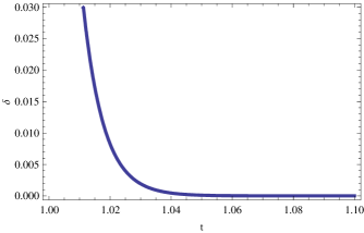
Figure 3: Behaviour of $\delta(t)$.

IV.3 Toy model

In this subsection, we are aiming to show that the situation can be even more complicated, with some subtleties which do not appear in what depicted above. For this purpose we present a toy model, which has the advantage of being simple and suitable for illustrating our claim. Thus, let us consider the unperturbed equations and assume that the evolution of $\varphi$ is given by $\varphi=t^{-1}$. From the well known relation

$$\dot{\varphi}^{2}=-2\dot{H}\,,$$ (33)

it is possible to derive

$$a=\exp\left(-\frac{1}{12t^{2}}\right)\,,$$ (34)

and it is also possible to arrive at the potential

$$V=\frac{1}{12}\varphi^{6}-\frac{1}{2}\varphi^{4}\,.$$ (35)

It is then easy to check that $V$ in (4.18) is again a special exact solution. We have now

$$\lim_{t\rightarrow\infty}(a^{3}\varphi^{2})=0\,,$$ (36)

so that $\dot{\theta}$ goes to infinity with time in this case (see Fig. 4). As a matter of fact, it appears to be divergent already at the time $t=3.5$, as shown in Fig. 4.

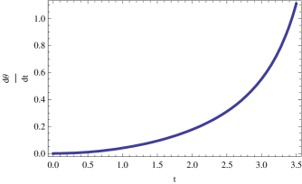
Figure 4: Behavior of $\dot{\theta}=d\theta/dt$ as a function of time $t$.

The expression of Eq. (4.17) is clearly inflationary for small $t$, because

$${\ddot{a}}=e^{-{1\over 12t^{2}}}{(1-18t^{2})\over 36t^{6}},$$ (37)

so that inflation actually ends at $t_{f}=\sqrt{18}$. Here, it has been allowed to start from the very beginning, in such a way that, the time scale being arbitrary, there is no problem with the e-folding number. On the other hand, our formula for the scale factor leads to

$$\lim_{t\to\infty}a(t)=1,$$

which is clearly unphysical, but we already acknowledged that it is only a toy model, which should be anyway taken more seriously into account only until the end of inflation.

Let us now consider the perturbed system. On going back to Eq. (4.1) we see that, for very small $a$, the term containing $Q$ can dominate and there is no inflation. In order to verify this, let us take as “initial” time $t_{f}=\sqrt{18}$, i.e. the time corresponding to the end of inflation, and let us integrate the Euler–Lagrange equations backwards in time. By assuming $Q=10^{-8}$, we obtain the plot of Fig. 5 for $\ddot{a}$.

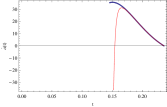
Figure 5: Plot of the time evolution of $\ddot{a}$, for both the exact (blue colored) and perturbed (red colored) scale factors $a(t)$, when the exponential potential given in Eq. (3.6) is used in the inflationary regime.

We see that indeed now one has a natural way for the beginning of inflation. This sounds interesting, but it is also clear that the duration is now too much shortened, and the e-folding turns out to be of order $1$! Of course, it is possible to improve the situation by taking a much smaller value for $Q$, so small that it is impossible to perform a numerical integration. This is a sort of fine tuning on the phase which should be investigated further. Eventually, we now go beyond the end of inflation, to the future of $t_{f}$. In Fig. 6 a double surprise is now obtained. First, we obtain a new limited period of accelerated expansion. This suggests, confirming in part what was found before in Sec. IV, that a complex scalar field might emulate dark energy, but of course this statement should be supported with much deeper investigation. Second, we obtain a singularity at $t\approx 37$. It is not clear whether this is due to numerical integration problems. Of course, a choice of a much smaller value for $Q$ would push these features to the right. But this is even more interesting because, by virtue of the time scale here adopted, this is just what is needed.

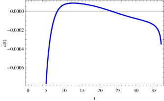
Figure 6: Plot of the time evolution of $\ddot{a}$, showing a short period of accelerated expansion after the end of inflation, with a possible singularity at a certain time.

V Semiclassical quantum cosmology with the potential of the form $V(\varphi)=\frac{1}{12}\varphi^{6}-\frac{1}{2}\varphi^{4}$

Since we have just found a strong motivation for studying the somewhat unusual potential in Eq. (35), we now take it again into account from a complementary point of view, i.e., the semiclassical approximation in quantum cosmology. For the basic references on this vast subject, and for a detailed discussion of the main issues, we refer the reader to Refs. HH83 ; H84 ; Espo88 ; Hall09 and to the many references therein.

In a minisuperspace approach to quantum cosmology, one may start from the point Lagrangian ruling the FLRW models, which, in dimensionless units and with the metric signature $(-\,+\,+\,+)$, reads as (to be consistent with all previous sections, our gravitational Lagrangian is $-6$ times the one in Ref. Espo88 )

$$L=-3a{\dot{a}}^{2}+3ka+{1\over 2}a^{3}{\dot{\varphi}}^{2}-a^{3}V(\varphi)\,,$$ (38)

where $k$ is positive, vanishing, negative, for closed, spatially flat and open universe models, respectively. The resulting classical Hamiltonian takes the form

$$H=-{1\over 12a}p_{a}^{2}+{1\over 2a^{3}}p_{\varphi}^{2}-3ka+a^{3}V(\varphi)\,,$$ (39)

where the conjugate momenta $p_{a}$ and $p_{\varphi}$ are given by

$$p_{a}\equiv{\partial L\over\partial{\dot{a}}}=-6a\dot{a}\,,\;p_{\varphi}\equiv{\partial L\over\partial{\dot{\varphi}}}=a^{3}{\dot{\varphi}}\,.$$ (40)

Now we use the hat symbol for the momentum and Hamiltonian operators of the quantum theory, and we adopt the following operator-ordering prescription Espo88 :

$${\hat{p}}_{a}^{2}\equiv-{1\over a}{\partial\over\partial a}\left(a{\partial\over\partial a}\right)=-{\partial^{2}\over\partial a^{2}}-{1\over a}{\partial\over\partial a}\,,$$ (41)

$${\hat{p}}_{\varphi}^{2}=-{\partial^{2}\over\partial\varphi^{2}}\,,$$ (42)

where, on defining $\alpha\equiv\log(a)$, one has

$${\partial\over\partial a}=e^{-\alpha}{\partial\over\partial\alpha}\,,$$ (43)

$${\partial^{2}\over\partial a^{2}}=e^{-3\alpha}\left({\partial^{2}\over\partial\alpha^{2}}-{\partial\over\partial\alpha}\right)\,,$$ (44)

and hence

$${\hat{H}}={1\over 2}e^{-3\alpha}\left({1\over 6}{\partial^{2}\over\partial\alpha^{2}}-{\partial^{2}\over\partial\varphi^{2}}\right)-3ke^{\alpha}+e^{3\alpha}V(\varphi)\,.$$ (45)

This operator can be written in a more symmetrical form by defining $\varphi\equiv\sqrt{6}\phi$, which yields a quantum cosmological wave function of the minisuperspace model depending only on the $\alpha,\phi$ variables and ruled by the Wheeler–DeWitt equation

$$\left[{\partial^{2}\over\partial\alpha^{2}}-{\partial^{2}\over\partial\phi^{2}}+12V(\sqrt{6}\phi)e^{6\alpha}-36ke^{4\alpha}\right]\psi(\alpha,\phi)=0\,.$$ (46)

In particular, in the spatially flat case, for which $k=0$, the phase $S$ of the JWKB ansatz $\psi(\alpha,\phi)\sim Ce^{iS}$ should obey the Hamilton–Jacobi equation

$$\left({\partial S\over\partial\phi}\right)^{2}-\left({\partial S\over\partial\alpha}\right)^{2}=-12V(\sqrt{6}\phi)e^{6\alpha}\,.$$ (47)

The comparison with the closed FLRW model studied in Ref. Espo88 suggests considering a factorized ansatz for $S$, i.e.

$$S(\alpha,\phi)=S_{1}(\alpha)S_{2}(\phi)\,.$$ (48)

Its insertion into Eq. (5.10) yields

$$\left({1\over S_{2}}{dS_{2}\over d\phi}\right)^{2}-\left({1\over S_{1}}{dS_{1}\over d\alpha}\right)^{2}=-{12V(\sqrt{6}\phi)\over S_{2}^{2}(\phi)}{e^{6\alpha}\over S_{1}^{2}(\alpha)},$$ (49)

which may be solved approximately by setting

$$S_{1}(\alpha)=-{e^{3\alpha}\over 3}\,,\;S_{2}(\phi)=\sqrt{12V(\sqrt{6}\phi)}\,,$$ (50)

and as a check Eq. (5.12) then takes the form

$${1\over V}{dV\over d\phi}=0\,.$$ (51)

If the potential (4.18) is assumed, the scalar field being real here for simplicity, one finds

$${1\over V}{dV\over d\phi}={2\over\phi}{(3\phi^{2}-2)\over(\phi^{2}-1)}\,,$$ (52)

and this does indeed vanish at large $\phi$.

Thus, if we assume that $\phi$ (and hence $\varphi$) takes initially a very large value $\phi_{0}={\varphi_{0}\over\sqrt{6}}$, we may use (5.11), (5.13) and (5.1) to study the first-order system

$$p_{a}={\partial S\over\partial a}={\partial L\over\partial{\dot{a}}}\,,\;p_{\phi}={\partial S\over\partial\phi}={\partial L\over\partial{\dot{\phi}}}\,,$$ (53)

about which the JWKB wave function is peaked Espo88 . Its explicit form reads as

$${d\alpha\over dt}=\sqrt{6}\phi^{2}\left(\phi^{2}-1\right)^{{1\over 2}}\,,$$ (54)

$${d\phi\over dt}=-\sqrt{{2\over 3}}{\phi(3\phi^{2}-2)\over\left(\phi^{2}-1\right)^{{1\over 2}}}\,.$$ (55)

Bearing in mind that $\phi$ must be very large in our approximation, these equations may be rewritten as

$${d\alpha\over dt}=\sqrt{6}\phi^{2},$$ (56)

$${d\phi\over dt}=-3\sqrt{{2\over 3}}\phi^{2}.$$ (57)

It is then immediate to obtain the solution at the end of Sec. IV, i.e.

$$\phi={\varphi\over\sqrt{6}}={1\over\sqrt{6}t},\;\alpha=-{1\over 12t^{2}}.$$ (58)

VI Conclusions

We think that we have illustrated how the introduction of a complex scalar field in the inflationary and/or quintessential scenario can be treated with simple and elegant procedures. In our opinion, the main results are:

(1) In our quintessence model, the phase of the field must be almost constant, so that the field may be safely treated as real.

(2) The situation is more involved in the inflationary scenario. It is then possible, as already pointed out by many authors, that the real field is obtained as a limit, by virtue of the increasing scale factor present in the denominator of Eq. (30). On the other hand, the introduction of the perturbing term may introduce a starting point for inflation, giving rise to some problems of fine tuning. Also the behavior after the end of inflation can be dramatically changed.

(3) The only possible symmetry of this situation turns out to be the trivial one, linked with the cyclic character of the phase. At this point the Noether symmetry approach has proved to be helpful. Even if the potential is here assumed to be a function of the modulus only, it has to be noted that other assumptions are found in the literature (for example, see Ref. wei05 , containing a good number of references about the possible basic ways to introduce a complex scalar field in standard cosmology). We have shown that this procedure also applies, giving again a cyclic phase, in the hessence case.

(4) It is puzzling that the symmetry, which is found for exponential potentials in the case of real fields, is spoiled by the presence of any tiny imaginary component. It is very difficult to argue on this particular point because, as stated in many previous papers, the physical meaning of this kind of Noether symmetries (which proved so fruitful for the solutions of many problems) is still mysterious for us. Perhaps one can argue that the Noether symmetry only applies to the background evolution, and has nothing to do with the actual symmetries of the full theory.

(5) The study of a toy model for the potential in Eq. (4.18), despite being somewhat “unphysical”, shows some intriguing issues, as well as some confirmation of what emerged in Sec. IV for the dark energy case.

(6) The semiclassical quantum cosmology analysis for the scalar-field potential in Eq. (35) has been obtained for the first time in the literature in Sec. V. The resulting field equations lead again to the solution at the end of Sec. IV when suitable approximations are taken into account. This way of supplementing the results of Sec. IV is important because, as suggested in Ref. hawk05 , the evolution of the universe might be semiclassical.

- (1) S. Kasuya, Phys. Lett. B 515, 121 (2001).
- (2) J.-A. Gu and W.-Y.P. Hwang, Phys. Lett. B 517, 1 (2001).
- (3) L.A. Boyle, R.R. Caldwell, and M. Kamionkowski, Phys. Lett. B 545, 17 (2002).
- (4) Y.-H. Wei, R.-G. Cai, and D.-F. Zeng, Classical Quantum Grav. 22, 3189 (2005).
- (5) W. Zhao and Y. Zhang, Phys. Rev. D 73, 123509 (2006).
- (6) R. de Ritis, G. Marmo, G. Platania, C. Rubano, P. Scudellaro, and C. Stornaiolo, Phys. Rev. D 42, 1091 (1990).
- (7) S. Capozziello, R. de Ritis, C. Rubano, and P. Scudellaro, Rivista del Nuovo Cimento 19(4), 1 (1996).
- (8) C. Rubano and P. Scudellaro, Gen. Relativ. Grav. 34, 307 (2002).
- (9) D. Wands, Multiple Field Inflation, Lect. Notes Phys. 738, 275–304 (2008).
- (10) B.A. Bassett, S. Tsujikawa, and D. Wands, Rev. Mod. Phys. 78, 537 (2006).
- (11) K.A. Malik and D. Wands, Phys. Rev D 59, 123501 (1999).
- (12) D.H. Lyth and A. Riotto, Phys. Rep. 314, 1 (1999).
- (13) S.A. Kim and A.R. Liddle, Phys. Rev. D 74, 023513 (2006).
- (14) R. Abraham and J. Marsden, Foundation of mechanics (Benjamin, New York, 1978).
- (15) G. Marmo, E.J. Saletan, A. Simoni, and B. Vitale, Dynamical systems. A differential geometric approach to symmetry and reduction (Wiley, New York, 1985).
- (16) G. Morandi, C. Ferrario, G. Lo Vecchio, G. Marmo, and C. Rubano, Phys. Rep. 188, 149 (1990).
- (17) C. Rubano, P. Scudellaro, E. Piedipalumbo, and S. Capozziello, Phys. Rev. D 69, 103510 (2004).
- (18) E.R. Harrison, Phys. Rev. D 1, 2726 (1970).
- (19) Ya.B. Zel’dovich, Mon. Not. R. Astr. Soc. 160, 1P (1972).
- (20) F. Lucchin and S. Matarrese, Phys. Rev. D 32, 1316 (1985).
- (21) J.B. Hartle and S.W. Hawking, Phys. Rev. D 28, 2960 (1983).
- (22) S.W. Hawking, Nucl. Phys. B 239, 257 (1984).
- (23) G. Esposito and G. Platania, Classical Quantum Grav. 5, 937 (1988).
- (24) J.J. Halliwell, “Introductory lectures on quantum cosmology”, arXiv:0909.2566 [gr-qc].
- (25) S.W. Hawking, Phys. Scripta T 117, 49 (2005).