Characterization of Solar Telescope Polarization Properties Across the Visible and Near-Infrared Spectrum

Accurate astrophysical polarimetry requires a proper characterization of the polarization properties of the telescope and instrumentation employed to obtain the observations. Determining the telescope and instrument Muller matrix is becoming increasingly difficult with the increase in aperture size of the new and upcoming solar telescopes. We have carried out a detailed multi-wavelength characterization of the Dunn Solar Telescope (DST) at the National Solar Observatory/Sacramento Peak as a case study and explore various possibilites for the determination of its polarimetric properties. We show that the telescope model proposed in this paper is more suitable than that in previous work in that it describes better the wavelength dependence of aluminum-coated mirrors. We explore the adequacy of the degrees of freedom allowed by the model using a novel mathematical formalism. Finally, we investigate the use of polarimeter calibration data taken at different times of the day to characterize the telescope and find that very valuable information on the telescope properties can be obtained in this manner. The results are also consistent with the entrance window polarizer measurements, opening very interesting possibilities for the calibration of future large-aperture solar telescopes such as the ATST or the EST.

1 Introduction

The observation of polarization in astrophysical objects allows us to measure magnetic fields in their environment or to learn about the physical conditions reigning in the regions where light is scattered into our line of sight. However, polarimetry is a very challenging technique because the signals to measure are typically very weak ($<1\%$ of the observed intensity) and because the telescope and instrumentation employed introduce spurious polarization. Most polarimeters have calibration optics to determine its polarimetric properties so that it is possible to remove the instrumental contamination from the observed signals. However, it is only possible to characterize the instrumentation downstream from the calibration optics. Ideally, one would like then to have calibration polarizers before the telescope primary mirror and covering the entire aperture. Unfortunately, this is impractical in most situations. Currently, only the Dunn Solar Telescope at the National Solar Observatory/Sacramento Peak Observatory (Sunspot, NM, USA), the German VTT at the Observatorio del Teide on the island of Tenerife and the Swedish Solar Telescope at the Observatorio del Roque de los Muchachos on the island of La Palma (both operated by the Instituto de Astrofísica de Canarias, Spain) have that capability (Skumanich et al., 1997; Beck et al., 2005; Selbing, 2005). Even in these three cases the operation of the telescope calibration devices is far from routine and it takes considerable effort and a full day (sometimes more) of continued observation.

The largest solar telescopes currently under operation do not exceed 1 m of aperture but the soon-to-be commissioned Gregor has 1.5 m (Volkmer et al., 2007) and plans already exist for the construction of two 4 m telescopes: the Advanced Technology Solar Telescope (ATST, Keller et al., 2002) and the European Solar Telescope (EST, Collados et al., 2010). With such large apertures, full telescope calibrations become extremelly challenging from a technical standpoint.

An additional problem is that the configuration of the telescope is not fixed. It has some degrees of freedom, e.g. to be able to point at different coordinates on the sky. When the telescope moves, the angles among some of the many mirrors and optical elements along the light path also change. In the case of solar observations there is typically a continuous variation of at least two mirrors as one tracks the apparent motion of the Sun on the sky. Therefore, it does not suffice to derive the Muller matrix at a given time. We need to know how it depends on the telescope configuration. In this manner, since we know the specific configuration at the time of each observation, we can use the correct Muller matrix to calculate the parasitic instrumental polarization induced and remove it from the data.

We shall follow here a similar nomenclature to that of Skumanich et al. (1997) and Socas-Navarro et al. (2006). We break down the polarimetric measurement process as:

$$\@vec{S}_{meas}=\@tens{X}\@tens{T}(\@vec{\alpha})\@vec{S}_{\sun}\,$$ (1)

where $\@tens{T}(\@vec{\alpha})$ is the telescope Muller matrix, $\@tens{X}$ denotes the polarimeter response, and $\@vec{S}_{\sun}$ and $\@vec{S}_{meas}$ are the incoming (solar) and the measured Stokes vectors, respectively. The polarimeter calibration optics (typically a combination of a polarizer and a retarder than can be slided in and out of the beam and rotated independently of each other) mark the split point of the optical train. Any optical surface upstream from that point is considered part of the telescope and included in $\@tens{T}$, whereas everything downstream is part of the polarimeter and characterized in $\@tens{X}$. We shall take the polarimeter as a static system since it has no moving parts, with only minor changes due to thermal fluctuations. The telescope, on the other hand, has a variable configuration, e.g. with moving mirrors to point and track across the sky. We parameterize the particular configuration in the vector $\alpha$.

Acquiring calibration data to constrain $\@tens{T}(\@vec{\alpha})$ is much more difficult and time-consuming than for $\@tens{X}$. This is due to two reasons: a)the fact that $\alpha$ (and therefore $\@tens{T}$) varies over the course of a day, and b)the solar beam has a much larger diameter at the entrance of the telescope than at the polarimeter. The first difficulty imposes the need to take calibration observations for at least a half day (but preferably more than that) to ensure appropriate coverage over the range of variation of the parameters in $\@vec{\alpha}$. The second problem is not insurmountable for currently existing 1 m aperture telescopes but the planend large aperture of the EST or the ATST will require new strategies (e.g., Socas-Navarro, 2005a, b).

In this paper we take the DST as a case study and analyze its polarimetric properties at many wavelengths spanning the visible and near-infrared (nIR) ranges of the spectrum. We start by building an improved model of the telescope with respect to what has been done in previous work. We then use a novel mathematical formalism to validate the degrees of freedom in the model. Finally, we use two different strategies to fit the various parameters and obtain a reliable multi-wavelength characterization of the telescope. One of such strategies makes use of data taken with entrance window polarizers in the beam, whereas the other uses solar data thus avoiding the need for polarizers filling the full telescope aperture. We conclude that both strategies produce consistent results, which opens new interesting perspectives for the calibration of future large-aperture facilities.

2 The telescope model

In observing mode, the DST has the following optical surfaces, which could in principle alter the polarization state of the solar light. In the order encountred by the incoming beam, we find:

• An entrance window (EW) used to keep the optical train evacuated. Mechanical stress on the window mount could make it act as a retarder with a small degree of retardation.

• A turret with two 1 m diameter mirrors that track the Sun and send the light down in the vertical direction to the primary mirror which is located underground. The first turret mirror moves in the elevation direction ($\gamma$) and the second in azimuth ($\phi$). These two angles are needed to define the telescope configuration and we take them as the first components of the configuration vector $\@vec{\alpha}$ introduced earlier. The turret is a heavily polarizing device, since the beam strikes both mirrors at a 45 degree angle of incidence.

• The primary mirror, which due to its near normal angle of incidence does not alter the light polarization significantly except for a 180 degree phase change.

• The exit window (XW), which marks the end of the evacuated optical train. Like the EW, this element could introduce some small degree of retardation in the beam (in general, different from that of the EW). The main mirror, the XW and the instrument platform can rotate rigidly to compensate for the diurnal solar image rotation on the instrument focal plane and/or to define the orientation of the spectrograph slit. Let us donte by $\psi$ the angle of this whole system, which is the third and last element of the configuration vector $\@vec{\alpha}$.

Behind the XW we have the polarimeter calibration optics and the polarimeter itself. Therefore, the above elements are all that we need to consider in our telescope model.

We model both windows as an ideal retarder whose retardation is a free parameter. The orientation of the retarder fast axis is also a free parameter. The turret mirrors are modeled taken their diattenuation ($r_{s}/r_{p}$) and retardance as free parameters and calculating the orientation of the plane of incidence from $\gamma$ and $\phi$. For the main mirror it is a good approximation to consider a perfectly symmetric reflection with no diattenuation and a 180-degree retardation. With these considerations in mind, we construct the total Muller matrix of the telescope as:

$$\@tens{T}(\gamma,\phi,\psi)=\@tens{D}_{XW}\@tens{M}_{Main}\@tens{R}_{Main-AZ}(\psi,\phi)\@tens{M}_{AZ}\@tens{R}_{EL}(\gamma)\@tens{M}_{EL}\@tens{D}_{EW}\,,$$ (2)

where $\@tens{D}$ denotes the Muller matrix of a retarder in the ($s,p$) reference frame (i.e., with the axes parallel and perpendicular to the incidence plane), $\@tens{M}$ is the matrix of a mirror and $\@tens{R}$ is a rotation of the coordinate frame from one element to the next. The subscripts $EL$, $AZ$ and $Main$ refer to the elevation and azimuth mirrors of the turret and the primary mirror, respectively. In the equation above we have only written down explicitly the dependence of the various matrices with the telescope configuration angles $\@vec{\alpha}$, but not with the free parameters.

The free parameters of the model are then the EW fast axis orientation and retardance, the elevation and azimuth mirrors diattenuation and retardance and the XW fast axis orientation and retardance. In addition to those six parameters, we also consider as a free parameter a rotation angle between the telescope and the polarimeter respective reference frames and finally, in the case that the entrance window calibration polarizer is used, the zero point of the calibration polarizer. This results in a total of 8 free parameters for a single-wavelength model. In the next section we present a formal justification that this number of free parameters is nearly optimal for the problem under consideration.

For a multi-wavelength characterization we take a somewhat different approach from that in Socas-Navarro et al. (2006). We have observed that the polynomial fit proposed in that work to the wavelength dependence of the various parameters is not always adequate, as it does not always capture the real polarimetric behavior of the optical elements. When the number of wavelengths observed increases, that model has difficulty fitting all the data. In view of the results presented in this paper, particularly those in section 4 below, it is easy to see that a third-order polynomial will not be able to reproduce the real behavior of the telescope at all wavelengths.

The new model that we propose in this work has a number of $4+4\times n_{\lambda}$ free parameters (where $n_{\lambda}$ is the number of wavelengths observed). The 4 wavelength-independent parameters are the EW and XW fast axis orientations, the telescope-polarimeter reference frame rotation and the offset of the EW polarizers with respect to our assumed zero point. The EW, XW retardances and the turret mirror diattenuations ($r_{s}/r_{p}$) and retardances are functions of wavelength. We take their value at the observed wavelengths as a free parameter. Intermediate values are obtained from linear interpolation. In this manner increasing $n_{\lambda}$ results in more free parameters but at the same time the amount of data is also largely increased.

3 Dimension analysis

In principle, even if one bases the model of the telescope on simple assumptions, it is possible that the final model contains too many free parameters that cannot be constrained by the observations. In such a case, when one fits the model parameters to a set of calibration observations, the model might not be representative of the general behavior of the telescope. Obviously, this is produced by the overfitting ability of a model with too many free parameters. This is particularly relevant when several parameters are degenerated, meaning that the variation of one parameter can be compensated to a great extent with variations in one or more of the other parameters.

Consequently, we analyze the intrinsic dimensionality of the model using the maximum-likelihood estimation developed by Levina & Bickel (2005) and applied with success by Asensio Ramos et al. (2007) to estimate the intrinsic dimensionality of spectro-polarimetric data. By intrinsic dimensionality we mean the number of free parameters that the $\@tens{T}$-matrix really depends on, taking into account that degeneracies introduce correlations between the parameters and reduce the dimensionality. Given $N$ vectors of dimension $M$ represented as $\@vec{x}_{i}$, the dimensionality is estimated by using the expression:

$$\hat{m}_{k}^{-1}=\frac{1}{N(k-1)}\sum_{i=1}^{N}\sum_{j=1}^{k-1}\log\frac{T_{k}(\mathbf{x}_{i})}{T_{j}(\mathbf{x}_{i})}.$$ (3)

where $T_{k}(\mathbf{x}_{i})$ represents the Euclidean distance between point $\mathbf{x}_{i}$ and its $k$-th nearest neighbor. The previous equation is only valid for $k>2$ and it depends on the number of neighbors that we select. In principle, this can be used to analyze variations of the intrinsic dimensionality at different scales, but our results are relatively constant with $k$. The computational cost of this method is mainly dominated by the calculation of the $k$ nearest neighbors for every point $\mathbf{x}_{i}$.

As an illustrative example, we have considered data generated with a polynomial function:

$$y(x)=\sum_{i=0}^{n-1}c_{i}x^{i}\,.$$ (4)

This function may be viewed as a non-linear model with $n$ free parameters (the $c_{i}$ coefficients). Our aim is to estimate the order of the polynomial just from the samples. Since we have generated the data for this experimient, we can then verify a posteriori that the results accurately yield the correct number. Three different experiments were carried out for polynomials of order 1, 2 and 3, respectively. For each value of $n$, we generate $N=10^{4}$ vectors composed of samples of the polynomial at $M=10$ different positions ($x$). The estimation of the dimensionality is shown in Fig 1 where $n$ indicates the number of coefficientes of the polynomial (i.e., the polynomial order is $n-1$). Note that the results converge towards the correct dimensionality for small number of neighbors (for large values, the results are sensitive to the finite and discrete nature of the grid). Further details of this procedure and more exhaustive tests can be found in Asensio Ramos et al. (2007). Here we simply intend to use this example to illustrate the application to the telescope model presented below, where instead of a simple polynomial we have the $\@tens{T}$-matrix constructed as indicated in Eq 2 above from its 8 free parameters. If we had correlations or degeneracies among these parameters, then the dimensionality of the data produced with the model would be less than the number of free parameters.

For the analysis of the telescope model we consider each Stokes parameter $Q$, $U$ and $V$ separately, and the $N$ vectors are built as follows. Let $N_{\mathrm{pol}}$ be the number of angles of the axis of our EW polarizers. Let $N_{\mathrm{ang}}$ be the number of combinations of azimuth, elevation and table angles that characterize the telescope configuration. For each combination of polarizer angle, azimuth, elevation and table angle, we propagate a Stokes vector representing unpolarized light through the telescope (with its EW polarizers) by multiplying $(1,0,0,0)\dagger$ by the full telescope Muller matrix $\@tens{T}$ (the symbol $\dagger$ represents the matrix transposition operation). Keeping the parameters of the matrix fixed, we construct the vector of length $M=N_{\mathrm{pol}}N_{\mathrm{ang}}=100$ by stacking the emergent Stokes parameter ($Q$, $U$ or $V$) for all the possible combinations. Each such vector then represents a realization of the observable that can be used to characterize the Mueller matrix of the telescope. This procedure is repeated $N$ times until the entire database is filled. Due to computational limitations in the $k$ nearest neighbors calculation, we limit ourselves to $N=10^{4}$ different values of the parameters. These values have been generated by means of a latin hypercube sampling (McKay et al., 1979), which produces a better sampling of the parameter space.

Figure 1: Dimensionality of three different polynomial models with 2, 3 and 4 coefficients. The curves converge to the correct degrees of freedom for a small number of neighbors.

Figure 2: Dimensionality of the telescope model with 8 free parameters described in Section 2. All Stokes parameters $Q$, $U$ and $V$ converge to a value of approximately 7.5, evidencing that the model does not have degerate parameters.

Figure 3: Dimensionality of the telescope model with 10 free parameters (the previous 8 plus main mirror diattenuation and retardance). All Stokes parameters $Q$, $U$, and $V$ converge to a value of approximately 8 even though we have 10 free parameters, evidencing that the model has degenerate parameters.

We have applied the dimension analysis on these data and obtained the results plotted in Fig 2. All of the Stokes parameters exhibit the same behavior and converge to approximately 7.5, which is very close to the number of free parameters (8, see Section 2) in our model. From this we can conclude that no significant degeneracies exist among the various free parameters and that a variation on each one of them produces an independent, measureable result on the observables. In other words, we can be confident that with enough data and a sufficient coverage of the configuration space, it is possible to univocally retrieve all of these parameters.

Our original model also had the main mirror diattenuation and retardance as free parameters. However, after a few attempts with different initializations, we quickly realized that there were uniqueness issues as we were able to fit the data with different combinations of the parameters. In particular, we found that the main mirror retardation exhibited a seemingly random wavelength dependence that was nearly identical (but opposite) to that of the XW. A quick look at the model (see Eq 2) shows that there are no other elements between the main mirror and the XW. Therefore, one can set any arbitrary value for the retardation in the main mirror and then compensate it with an opposite retardation in the XW. We explored this issue with the dimension analysis, this time having 10 free parameters in the model (the previous 8 plus the main mirror diattenuation and retardance). The results are plotted in Fig 3. Note that, even though we now have more free parameters, the dimensionality of the data has not changed significantly and we obtain again a result close to 8. This indicates that this model now has too much freedom and some of the free parameters are degerate. We thus decided to fix the main mirror properties to those of a non-polarizing reflection, which is a good approximation anyway based on symmetry considerations.

4 Entrance window polarizers

The DST is equipped with an array of achromatic linear polarizers that can be mounted on top of the EW. The entire array may be rotated in azimuth to any desired angle by means of a system consisting of a motor and its associated control electronics. With this device it is possible to feed the telescope with light in a known state of polarization and probe the properties of the full optical train, from the EW to the polarimeter.

In addition to the EW polarizers we also have the regular polarimeter calibration optics with which it is possible to fully characterize the instrument (in our case, SPINOR). We start the process by determining the SPINOR response matrix which we then fix in the determination of the telescope properties. This is a routine operation that involves inserting the SPINOR calibration polarizer and retarder and rotating them independently to various angles. After going through the calibration polarizer, the previous state of polarization becomes irrelevant as the light will then become fully polarized in the direction set by the polarizer (the total light intensity is also irrelevant since we work with normalized Stokes vectors and consider only the degree of linear/circular polarization). The polarimeter calibration is then independent of the telescope configuration ($\alpha$).

It is important to have the polarimeter characterized first, othwerwise we would have to fit also the matrix $\@tens{X}$ and there would be too many free parameters with unpleasant couplings between some of the optical elements. On 2010 May 3 we performed a total of 21 polarimeter calibration operations at different times during the day. In each one of these operations we recorded a sequence of 76$\times$8 images (76 configurations of the calibration optics and 8 modulation states) with a cross-dispersing prism placed in front of the detector, removing the order isolation pre-filter and blocking most of the spectrograph slit length to allow only a small field of view in the spatial direction. After proper demodulation, the 8 images in the modulation sequence are transformed into 4 containing at each pixel the Stokes $I$, $Q$, $U$ and $V$ parameters. Each image contains a number of spectral ranges (9 in our case) that span the entire visible and nIR range, as shown in the example of Fig 4.

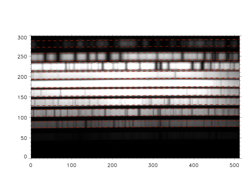
Figure 4: Example of a calibration image with the cross-dispersed spectral orders. Each band enclosed with dashed lines represents one of the overlapping orders in the spectrograph (order-isolation filters are removed for these operations) that we have used for this work, ranging from 470 (bottom) to 1413 (top) nm. Spectral lines are visible in the data. The central orders have been saturated in the figure to show the weaker ones at the top and the bottom.

We employ a Levenberg-Marquardt (see, e.g. Press et al. 1986) algorithm to fit the Stokes data to a model with a 4$\times$4 response matrix. Since the calibration retarder is not a perfect $\lambda$/4 plate over the entire wavelength range, we also take its retardance as a free parameter and determine it from the fit. The orientation of the retarder fast axis is also a free parameter to correct for possible errors in the mount alignment. All the Stokes vectors are normalized to their respective intensity so only their orientation in the Poincaré sphere is considered. As a result, the $\@tens{X}_{(1,1)}$ matrix element will always be equal to 1.

Figures 5 and 6 show the resulting polarimeter properties as a function of wavelength obtained as described above. In Fig 5 we can see the properties of the calibration retarder. Since the retarder is not perfectly achromatic, there is a variation of its retardance (Fig 5, upper panel). The difference between the orientation of the retarder fast axis and its reference zero-point is also fitted (Fig 5, lower panel). As expected this difference is very small, below a few degrees in any case.

Figure 6 shows the 16 elements of the $\@tens{X}$ matrix as a function of wavelength. As mentioned above, we have repeated the measurements 21 times at different times of the day. Both figures are actually showing all 21 curves overplotted. The differences among them are so small in most cases that all of these curves virtually coincide (although the spread seems to increase for the greatest wavelengths). This impressive agreement reinforces our degree of confidence in the methodology that we have employed, since each one of the 21 curves was obtained from independent measurements that were also fitted independently. Furthermore, it also indicates that SPINOR exhibits a very high degree of temporal stability in its polarimetric properties.

Figure 5: Properties of the polarimeter (SPINOR) calibration retarder as a function of wavelength. Upper panel: Retardance. Lower panel: Difference between the retarder fast axis orientation and the mount zero point. In both cases we have overplotted all 21 curves obtained from the (independent) calibration measurements carried out over the course of a day.

Figure 6: Elements of the polarimeter (SPINOR) 4$\times$4 response matrix as a function of wavelength. In all panels we have overplotted all 21 curves obtained from the (independent) calibration measurements carried out over the course of a day.

Now that we have the elements of $\@tens{X}$ and we can fix that part of the equation, we turn to the telescope itself. With the EW polarizer in the beam, we acquired data during the afternoon of 2010 May 3 and also during the following day. A total of 15070 Stokes vectors were recorded at each one of the 9 wavelengths considered (the same wavelengths that had been observed before during the polarimeter calibration) and for different telescope configurations, which was continuously tracking the Sun on the sky and also moving the DST rotating platform to different angles.

Figure 7: Wavelength-dependent parameters obtained for the telescope model. The dashed lines represent the properties of a non-polarizing element, such as the DST primary mirror in our model.

Similarly to the polarimeter characterization above, we applied a computer-intensive Levenberg-Marquard fit to the entire dataset using the telescope model described in Section 2. The results are summarized in Fig 7 (wavelength-dependent parameters) and in Table 1 (wavelengt-independent parameters). Comparing Fig 7 to Fig 5 of Socas-Navarro et al. (2006) one can see where the problems with the previous model come from. The third-order polynomials can adequately reproduce the behavior that we find here for the EW and XW retardances and also the turret retardance. However, the turret $r_{s}/r_{p}$ is not properly described and, for some wavelengths, it departs significantly.

Table 1: Telescope wavelength-independent parameters from the model fit.

$$\begin{array}[]{p{0.5\linewidth}l}\hline\cr\vskip 3.0pt plus 1.0pt minus 1.0pt\cr Parameter&Value\\ &(degrees)\\ \vskip 3.0pt plus 1.0pt minus 1.0pt\cr\hline\cr\vskip 3.0pt plus 1.0pt minus 1.0pt\cr EW fast axis orientation&138.29\\ XW fast axis orientation&42.76\\ Telescope-SPINOR frame rotation&93.17\\ EW polarizer zero offset&81.53\\ \vskip 3.0pt plus 1.0pt minus 1.0pt\cr\hline\cr\end{array}$$

We can see in Fig 7 that the various elements behave monotonically, with a trend for the instrumental polarization to decrease towards longer wavelengths (note, however, that even in the nIR the telescope elements polarize significantly). The only exception is the diattenuation of the turret mirrors, which exhibits a peak around 850 nm. This peak is to be expected for an aluminum-coated mirror. Theoretical models of the mirrors show a qualitatively similar behavior with the 850 nm peak. The actual details depend on the thickness of the Al₂O₃ layer deposited on the mirror substrate but some ilustrative examples are given in Fig 8. The details of the calculation can be found in Born & Wolf (1975).

Figure 8: Theoretical calculation of an aluminum mirror diattenuation (upper panel) and retardance (lower panel) as a function of wavelength. The four curves represent different values for the thickness of the oxide layer. From top to bottom: 10, 20, 50 and 80 nm, respectively. The curves for 10 and 20 nm overlap in the upper panel. The diamonds show the values obtained from our fit for the turret mirrors (see Fig 7)

5 Polarimeter calibration optics

When incoming unpolarized light goes through the telescope system, it becomes partly polarized. The state of polarization depends on the telescope configuration $\alpha$. It is then possible to obtain information on the telescope properties by simply monitoring how the transfer from Stokes $I$ to $Q$, $U$ and $V$ changes over the course of the day. Such measurement can in principle be carried out without resorting on polarizers filling the entire telescope aperture, as done in Section 4. We can use the polarimeter calibration optics at the exit port of the telescope to measure the outgoing Stokes vector produced from a raw unpolarized solar beam.

The main polarization creation device is the turret, which introduces both diattenuation and retardation in the unpolarized beam. The resulting partly polarized beam further undergoes an additional retardation by the XW. The main mirror contributes negligibly, as mentioned above, because of the near normal incidence. Finally, the retardance introduced by the EW on an unpolarized incoming beam is also irrelevant. Based on these considerations, it is easy to see that this method will not provide information on the EW or the main mirror properties but one may hope to learn something about all the other elements.

Figure 9 shows the results of fitting all the calibration operation data acquired over the course of a day to the telescope model. The results are compatible with the measurements using the EW polarizer presented in Section 4. The turretm mirror properties are much better constrained than those of the EW, as one would expect since they polarize the incoming beam much more strongly than the XW.

Figure 9: Fit to the data with the polarimeter calibration optics (diamonds) compared to the model obtained with the EW polarizer (dashed line).

6 Conclusions

Calibrating the instrumental polarization of large solar telescopes is going to be an important challenge in the near future, especially for multi-wavelength observations. A key part of the process is the parametrization of the system in terms of a geometrical model with a few free parameters which are determined by fitting large calibration datasets. One needs to make sure that the model chosen has the right number of free parameters. With too much freedom one is able to fit the data but the model obtained is not unique and the properties of the individual components are unreliable. Too little freedom, on the other hand, limits the ability of the model to fit the calibration data and results in an inaccurate calibration. We have presented here a robust model for the DST telescope. Our dimension analysis, together with the model’s ability to fit all the data at all wavelengths, shows that it has the correct amount of freedom.

The technique based on EW polarizers is the most straightforward and accurate way to characterize the polarimetric properties of a telescope. However, we have shown that, when this is not practical, it is also possible to use the calibration optics downstream to constrain the model parameters (at least those related to the most heavily polarizing elements) if a sufficiently large collection of calibration data is acquired. These results are encouraging and open new possibilities for accurate broadband characterization of future large-aperture telescopes.