Mathematical analysis of a two-dimensional population model of metastatic growth including angiogenesis.

Abstract

Angiogenesis is a key process in the tumoral growth which allows the cancerous tissue to impact on its vasculature in order to improve the nutrient’s supply and the metastatic process. In this paper, we introduce a model for the density of metastasis which takes into account for this feature. It is a two dimensional structured equation with a vanishing velocity field and a source term on the boundary. We present here the mathematical analysis of the model, namely the well-posedness of the equation and the asymptotic behavior of the solutions, whose natural regularity led us to investigate some basic properties of the space $W_{\rm div}(\Omega)=\{V\in L^{1};\;{\rm div}(GV)\in L^{1}\}$, where $G$ is the velocity field of the equation.

AMS 2010 subject classification: 35A01, 35B40, 35B65, 47D06, 92D25.

Keywords : 2D structured populations, semigroup, asymptotic behavior, malthus parameter, transport equation.

1 Introduction

In the seventies, Judah Folkman puts forward the assumption that a cancer tissue, like other tissues, needs nutrients and oxygen conveyed by the blood vessels. Consequently, tumoral growth and development of metastasis are dependent on angiogenesis, a process consisting in building and developing the vascularization. From this discovery, a new anti-cancer therapeutic way is open : to starve cancer by depriving it of its vascularization. If for the last two decades, more than ten antiangiogenics drugs have been developed, mainly monoclonal antibodies and tyrosin kinase inhibitors, the administration protocols are far from being optimal. It is enough for example to consult the publication [13] to realize the paroxystic effects they can induce.

Thus, a tool for in silico studying the administration protocols for antiangiogenic drugs could largely contribute to optimize the effectiveness of the treatments, in particular to avoid some therapeutic failures. In this direction, the construction of a mathematical model taking into account the mechanisms of tumoral angiogenesis and the effect of the antiangiogenics agents proves to be an essential stage in order to improve the use of antiangiogenic therapies. Some work (for example in [22] and [5]) was made with the aim of qualitatively studying the effects of antiangiogenic therapies on the control of the primitive tumor growth. In this work we propose a modeling which purpose is to describe the action of the currently used clinical protocols, not only on the tumoral growth, but also on the production of metastases.

The model is a combination of the PDE model for the metastasis density proposed by [17] and studied in [3, 9], with the ODE model for each metastasis’ growth of Folkman et al. [16]. This transport equation endowed with a non-local boundary condition expressing creation of metastasis can be classified as part of the so-called structured population equations arising in mathematical biology which have the following general expression

(4) $$\left\{\begin{array}[]{ll}{\partial}_{t}\rho+{\rm div}(F(t,X,\rho))=-\mu(t,X,\rho)&\Omega\\ -G\cdot\overrightarrow{\nu}\rho(t,\sigma)=B(t,\sigma,\rho)&\sigma\in{\partial}\Omega\;s.t.\;G\cdot\overrightarrow{\nu}(\sigma)<0\\ \rho(0,X)=\rho^{0}(X)&\Omega\end{array}\right..$$

The introduction of such equations in the linear case is due to Sharpe and Lotka in 1911 [24] and McKendrick in 1926 [18]. Although these equations have been widely studied both in the linear and nonlinear cases (for an introduction to the linear theory see the book of Perthame [20] and to the nonlinear one see the book of Webb [27], as well as [21] for a survey), a complete general theory has not been achieved yet, even in the linear case. Indeed, most of the models have the so called structuring variable $X$ being one-dimensional and often representing the age, thus evolving with $F(t,a,\rho)=\rho$. A difficulty on the regularity of solutions is introduced when the velocity is non-constant and vanishes (see [3, 9]). Dealing with situations in dimensions higher than one is not a common thing.

In our case, the model is a linear equation, with

$$F(t,X,\rho)=G(X)\rho$$

structured in two variables : $X=(x,\theta)$ with $x$ the size of metastasis and $\theta$ the so-called “angiogenic capacity”. The velocity field $G$ vanishes on the boundary of the domain, which is a square. Moreover, we have an additional source term in the boundary condition of the equation :

$$-G\cdot\overrightarrow{\nu}\rho(t,\sigma)=N(\sigma)\int\beta(X)\rho(t,X)+f(t,\sigma).$$

As far as we now, the mathematical analysis for multi-dimensional models is done only in situations where one of the structured variables is the age and thus with the first component of $G$ being constant (see for instance [26, 1, 11]). In the context of the follicular control during the ovarian process, a nonlinear model structured in dimension two with both components of the velocity field $G$ being non-constant is introduced in [14] but no mathematical analysis is performed due to the complexity of the model.

In the present paper, we address the problem of the mathematical analysis of our model, namely : existence, uniqueness, regularity and asymptotic behavior of the solutions. Following the method used in [2] and [3], we use a semigroup approach to deal with the existence and regularity of the solutions. The main difficulties we have to deal with in this two dimensional problem come from the singularity of the velocity field, as well as the presence of a time-dependent source term in the boundary condition. During the study, we take a particular attention on the problems of regularity of the solutions and approximation of weak solutions by regular ones, which led us to study the space $W_{\rm div}(\Omega)$ (see the appendix) . The paper is organized as follows : in the section 2 we present the model, in the section 3 we study the properties of the underlying operator and in the section 4 we apply our study to the evolution equation from our model.

2 Model

The model we developed is an improvement of the model proposed by [17] and studied in [3]. We want now to take into account the key process of angiogenesis in the tumoral growth and integrate it in the metastatic evolution. To do this, we combine a renewal equation describing the evolution of the density of metastasis with an ODE model of tumoral growth including angiogenesis developed by Hahnfeldt et al. in [16].

2.1 The ODE model of tumoral growth under angiogenic control

We present now the model of Hahnfeldt et al. from [16]. Let $x(t)$ denote the size of a given tumor at time $t$. The growth of the tumor is modeled by a gompertzian growth rate, which expression is :

(5) $$g_{1}(x)=ax\ln\left(\frac{\theta}{x}\right),$$

where $a$ is a parameter representing the velocity of the growth and $\theta$ the carrying capacity of the environment. The idea is now to take $\theta$ as a variable of the time, representing the degree of vascularization of the tumor and called ”angiogenic capacity”. The variation rate for $\theta$ derived in [16] is :

(6) $$g_{2}(x,\theta)=cx-d\theta{x}^{\frac{2}{3}},$$

If we denote $X(t)=\left(x(t),\theta(t)\right)$ and define $G(X)=\left(g_{1}(x,\theta),g_{2}(x,\theta)\right)$ we have the following system of ODE modeling the tumoral growth :

(11) $$\left\{\begin{array}[]{l}\frac{dX}{dt}=G(X)\\ X(t_{0})=\left(\begin{array}[]{c}x^{0}\\ \theta^{0}\end{array}\right)\end{array}\right.$$

In the figure 1, we present some numerical simulations of the phase plan of the system.

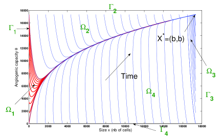
Figure 1: Phase plan of the ODE system (11).

This system has been studied by A. d’Onofrio and A. Gandolfi in [10]. We define

$$b=\left(\frac{c}{d}\right)^{\frac{3}{2}},\;\Omega=(1,b)\times(1,b),\;\Gamma={\partial}\Omega$$

We will now turn our interest to the flow defined by the solutions of the system of ODE, as it will play a fundamental role in the sequel. We define the application

$$\Phi:\begin{array}[]{ccc}[0,\infty[\times\Gamma&\rightarrow&\overline{\Omega}\\ (\tau,\sigma)&\mapsto&\Phi_{\tau}(\sigma)\end{array}$$

as being the solution of the system (11) at time $\tau$ with the initial condition $\sigma$. We use of this application in order to see $\Omega$ as $\Omega\simeq\;]0,\infty[\times\Gamma.$ More precisely, we will show that $\Phi$ is an homeomorphism locally bilipschitz $]0,\infty[\times\Gamma^{*}\rightarrow\Omega$ where $\Gamma^{*}:=\Gamma\backslash\{(b,b)\}.$ In order to have a candidate for the inverse of $\Phi$, we define for $(x,\theta)\in\Omega$

$$\begin{array}[]{c}\tau(x,\theta)=\rm{inf}\{\tau\geq 0|\;\Phi_{-\tau}(x,\theta)\in\Gamma^{*}\}\\ \sigma(x,\theta)=\Phi_{-\tau(x,\theta)}(x,\theta)\end{array}$$

The qualitative properties of the ODE imply the existence of such a couple $(\tau,\sigma)$ (the field points inward along $\Gamma^{*}$ and the solutions all converge to $X^{*}$ (see [10]) so going back in time they meet the boundary), and the Cauchy-Lipschitz theorem implies uniqueness because the system is autonomous and thus the characteristics don’t cross each other in the phase plane. The time $\tau(x,\theta)$ is the time spent in $\Omega$ and $\sigma(x,\theta)$ is the entrance point of the characteristic passing through the point $(x,\theta)$. From the Lipschitz regularity of $\Omega$ we can’t expect $\Phi$ to be globally ${\mathcal{C}}^{1}$, this is why we introduce the following open sets :

$$\Omega_{i}=\{\Phi_{\tau}(\sigma);\;\sigma\in\Gamma_{i},\,\tau\in]0,\infty[\},\quad i=1,2,3,4$$

where

$$\Gamma_{1}=](1,1),(1,b)[,\;\Gamma_{2}=](1,b),(b,b)[,\;\Gamma_{3}=](b,b),(b,1)[,\;\Gamma_{4}=](b,1),(1,1)[$$

The restriction of $\Phi$ to $]0,\infty[\times\Gamma_{i}$ is a diffeomorphism, as established in the following proposition.

Proposition 2.1 (Properties of the flow).

(i) The application $\Phi$ is a diffeomorphism $]0,\infty[\times\Gamma_{i}\rightarrow\Omega_{i}$ and for every $\tau\geq 0$ and almost every $\sigma\in\Gamma$

(12) $$J_{\Phi}(\tau,\sigma)=G\cdot\overrightarrow{\nu}(\sigma)e^{\int_{0}^{\tau}{\rm div}(G(\Phi_{s}(\sigma)))ds}$$

where $J_{\Phi}(\tau,\sigma)$ is the Jacobian of $\Phi$.
(ii) Globally, $\Phi$ is an homeomorphism $]0,\infty[\times\Gamma^{*}\rightarrow\Omega$ locally bilipschitz.

Remark 1.

The regularity proven here on $\Phi$ validates the use of $\Phi$ as a change of variables (see [12] for locally Lipschitz changes of variables).

Proof.

$\bullet$ $\Phi$ is one-to-one and onto. Let $X=(x,\theta)\in\Omega$. We have $\Phi(\tau(X),\sigma(X))=X$ because $\Phi_{-\tau(X)}(X)=\sigma(X)$ implies $X=\Phi_{\tau(X)}(\sigma(X))$ (indeed $\Phi_{-\tau}$ is the inverse of $\Phi_{\tau}$ when $\tau$ is fixed). In the same way, $(\tau(\Phi_{\tau}(\sigma)),\sigma(\Phi_{\tau}(\sigma)))=(\tau,\sigma)$. Thus $\Phi$ is one-to-one and onto and $\Phi^{-1}(x,\theta)=(\tau(x,\theta),\sigma(x,\theta))$.
     $\bullet$ $\Phi$ is a diffeomorphism on $]0,\infty[\times\Gamma_{i}$. Using the general theorem of dependency on the initial conditions for ODEs, $\Phi$ is ${\mathcal{C}}^{1}(]0,\infty[\times\Gamma_{i})$ and if we call $\sigma(s)$ a parametrization of $\Gamma_{i}$, we have $\frac{{\partial}\Phi}{{\partial}s}(\tau,\sigma(s))=D_{y}\Phi_{\tau}(\sigma(s))\circ\sigma^{\prime}(s)$, and the following characterization of $\frac{{\partial}\Phi}{{\partial}s}(\tau,\sigma(s))$ stands : for each $s$, it is the solution of the differential equation

$$\left\{\begin{array}[]{l}\frac{dZ}{d\tau}=DG(\Phi)\circ Z\\ Z(0)=\sigma^{\prime}(s)\end{array}\right.$$

Using this characterization, we can derive the formula (12) for the Jacobian $J_{\Phi}(\tau,\sigma)$. We have $J_{\Phi}(\tau,\sigma)=\frac{{\partial}\Phi}{{\partial}s}\wedge\frac{{\partial}\Phi}{{\partial}\tau}=\frac{{\partial}\Phi}{{\partial}s}\wedge G(\Phi)$, and differentiating in $\tau$, we get

$$\frac{{\partial}}{{\partial}\tau}J_{\Phi}(t,\sigma) =DG\circ\frac{{\partial}\Phi}{{\partial}s}\wedge G(\Phi)+\frac{{\partial}\Phi}{{\partial}s}\wedge DG\circ G(\Phi)$$

$$={\rm trace}(DG)J_{\Phi}(t,\sigma)={\rm div}(G)J_{\Phi}(t,\sigma)$$

Hence, for all $\sigma(s)$, using that $J_{\Phi}(0,\sigma(s))=\sigma^{\prime}(s)\wedge G(\sigma(s))=|\sigma^{\prime}(s)|G\cdot\overrightarrow{\nu}(\sigma(s))\neq 0,$ we obtain the formula

(13) $$J_{\Phi}(t,\sigma(s))=|\sigma^{\prime}(s)|G\cdot\overrightarrow{\nu}(\sigma(s))\exp(\displaystyle\int_{0}^{t}{\rm div}(G(\Phi(\tau,\sigma(s))))d\tau)\neq 0$$

We get (12) by choosing a parametrization with velocity equal to one.

Remark 2.

In the sequel, we fix this parametrization

We can then apply the global inversion theorem to conclude that $\Phi$ is a ${\mathcal{C}}^{1}$-diffeomorphism $]0,\infty[\times\Gamma_{i}\rightarrow\Omega_{i}$.
     $\bullet$ Globally. From the given properties of the vector field $G$, we can extend the flow to a neighborhood $V$ of $\overline{\Omega}$, and we have that it is ${\mathcal{C}}^{1}(]0,\infty[\times V)$ (see [8], XI p.305). Hence $\Phi$, which is the restriction of this application to $]0,\infty[\times\Gamma^{*}$ with $\Gamma^{*}$ being Lipschitz, is locally Lipschitz. Remark here that it is not globally Lipschitz since $\frac{{\partial}}{{\partial}\sigma}\Phi_{\tau}(\sigma)$ can blow up when $\tau$ goes to infinity, due to the singularity at $X^{*}$.
     To show that $\Phi^{-1}$ is also locally Lipschitz on $\Omega$ we consider some compact set $K\subset\Omega$ and show that $\Phi^{-1}$ is Lipschitz on $K$. We define $K_{i}=\overline{\Omega_{i}}\cap K$, and $\widetilde{K_{i}}:=\Phi^{-1}(K_{i})\subset]0,\infty[\times\overline{\Gamma_{i}}$. Now since $\Phi$ is the restriction of a globally ${\mathcal{C}}^{1}$ application, we have $\Phi\in{\mathcal{C}}^{1}(\widetilde{K_{i}})$, meaning that its differential $D\Phi$ is continuous until the boundary of $\widetilde{K_{i}}$. Moreover using the formula (13), we see that the value of $D\Phi$ on ${\partial}\widetilde{K_{i}}$ is invertible since we avoid the singularity $X^{*}$. Hence, using the continuity of the inverse application we obtain that $D\Phi^{-1}=(D\Phi)^{-1}$ is continuous on $K_{i}$. Thus $\Phi^{-1}\in{\mathcal{C}}^{1}(K_{i})$ and so it is Lipschitz on each $K_{i}$. As the global continuity of $\Phi^{-1}$ on $\Omega$ is deduced from the continuity on $\Omega$ of $X\mapsto\tau(X),$ it is Lipschitz on $K$. ∎

2.2 A renewal equation for the density of metastasis

Starting from the velocity field $G$ of the previous subsection for one given tumor, we now derive a renewal equation for the density $\rho(t,x,\theta)$ of metastasis at time $t$, size (= number of cells) $x$ and so called ”angiogenic capacity” $\theta$. The term density for $\rho$ means that the number of metastasis at time $t$ in an infinitesimal volume centered in $(x,\theta)$ and of size $dxd\theta$ is $\rho(t,x,\theta)dxd\theta$. We assume that each metastasis evolves in the space $(x,\theta)$ with the velocity $G(x,\theta)$. Expressing the conservation of the number of metastasis, we obtain

(14) $${\partial}_{t}\rho+{\rm div}(\rho G)=0.$$

The metastasis cannot have size nor angiogenic capacity bigger than the parameter $b$, and we assume them to have size and angiogenic capacity bigger than $1$. We are thus driven to consider the transport equation (14) in the square $\Omega=(1,b)\times(1,b)$. The field $G$ pointing inward all along the boundary, we need now to precise the boundary condition on $\Gamma$.
     Metastasis do not only grow in size and angiogenic capacity, they are also able to emit new metastases. We denote by $\beta(x,\theta,\sigma)$ the birth rate of new metastasis with size and angiogenic capacity $\sigma\in\Gamma$ by metastasis of size $x$ and angiogenic capacity $\theta$, and by $f(t,\sigma)$ the term corresponding to metastasis produced by the primary tumor. Expressing the equality between the entering flux of metastasis and the number of new born, we derive the following boundary condition on $\Gamma$ :

$$-G\cdot\overrightarrow{\nu}(\sigma)\rho(t,\sigma)=\int_{\Omega}\beta(x,\theta,\sigma)\rho(t,x,\theta)dxd\theta+f(t,\sigma)$$

We then assume that there is no coupling between $(x,\theta)$ and $\sigma$ in the expression of $\beta$, which is traduced by an expression of $\beta$ as $\beta(x,\theta,\sigma)=N(\sigma)\beta(x,\theta)$. Now let $\;Q:=]0,+\infty[\times\Omega,\;\Sigma:=]0,+\infty[\times\Gamma$. The equation is

(18) $$\left\{\begin{array}[]{ll}{\partial}_{t}\rho+{\rm div}(G\rho)=0&\forall\,(t,x,\theta)\in Q\\ -G\cdot\overrightarrow{\nu}\rho(t,\sigma)=N(\sigma)\int_{\Omega}\beta(x,\theta)\rho(t,x,\theta)dxd\theta+f(t,\sigma)&\forall\,(t,\sigma)\in\Sigma\\ \rho(0,x,\theta)=\rho^{0}(x,\theta)&\forall\,(x,\theta)\in\Omega\par\end{array}\right.$$

We will do the following assumptions on the data :

$$\beta\in L^{\infty},\;\beta\geq 0\;a.e.,\;N\in Lip(\Gamma)\text{ with compact support in $\Gamma^{*}$},\;N\geq 0,\;\int_{\Gamma}N=1$$

(19) $$G\text{ given by \eqref{g1} and \eqref{g2}}$$

Remark 3.

In practice, the new metastasis only appear with size $1$ and there should not exist metastasis on $\Gamma_{2,3,4}$, thus in the biological model we have ${\rm supp}(N)\subset\Gamma_{1}$. The expression of $\beta$ we use in the biological applications is $\beta(x,\theta)=mx^{\alpha}$ with $m$ and $\alpha$ two positive parameters traducing respectively the aggressiveness of the cancer and the spatial organization of the vasculature. The source term $f$ has the following expression in biological applications : $f(t,\sigma)=N(\sigma)\beta(X_{p}(t))$ with $X_{p}(t)$ representing the primary tumor and being solution of the system (11).

Definition 2.1 (Weak solution).

Let $\rho^{0}\in L^{1}(\Omega)$ and $f\in L^{1}(]0,\infty[\times\Gamma)$. We call weak solution of the equation (18) any function $\rho\in{\mathcal{C}}([0,\infty[;L^{1}(\Omega))$ which verifies: for every $T>0$ and every function $\phi\in{\mathcal{C}}^{1}_{c}([0,+\infty[\times\overline{\Omega}^{*})$

(20) $$\int_{0}^{T}\int_{\Omega}\rho[{\partial}_{t}\phi+G\cdot\nabla\phi]dtdxd\theta+\int_{\Omega}\rho^{0}(x,\theta)\phi(0,x,\theta)dxd\theta$$

$$-\int_{\Omega}\rho(T,x,\theta)\phi(T,x,\theta)dxd\theta-\int_{0}^{T}\int_{\Gamma}N(\sigma)\left(\int_{\Omega}\beta(x,\theta)\rho(t,x,\theta)dxd\theta\right)\phi(t,\sigma)d\sigma dt=0$$

Analyzing the equation (18) indicates that the solution is the sum of two terms : an homogeneous one associated to the initial condition, which solves the equation without the source term $f$ (which we will refer to as the homogeneous equation)

(24) $$\left\{\begin{array}[]{ll}{\partial}_{t}\rho+{\rm div}(G\rho)=0&\forall\,(t,x,\theta)\in Q\\ -G\cdot\overrightarrow{\nu}\rho(t,\sigma)=N(\sigma)\int_{\Omega}\beta\rho(t)dxd\theta&\forall\,(t,\sigma)\in\Sigma\\ \rho(0,x,\theta)=\rho^{0}(x,\theta)&\forall\,(x,\theta)\in\Omega\par\end{array}\right.$$

and a non-homogeneous term associated to the contribution of the source term $f(t,\sigma)$ and solution to the equation (which will be refered as the non-homogeneous equation)

(28) $$\left\{\begin{array}[]{ll}{\partial}_{t}\rho+{\rm div}(G\rho)=0&\forall\,(t,x,\theta)\in Q\\ -G\cdot\overrightarrow{\nu}\rho(t,\sigma)=N(\sigma)\int_{\Omega}\beta\rho(t)dxd\theta+f(t,\sigma)&\forall\,(t,\sigma)\in\Sigma\\ \rho(0,x,\theta)=0&\forall\,(x,\theta)\in\Omega\end{array}\right.$$

For existence and uniqueness of solutions, we will deal with the homogeneous problem using the semigroup theory and with the non-homogeneous one via a fixed point argument.

2.3 Semigroup formulation for the homogeneous problem

We reformulate (24) as a Cauchy problem

(31) $$\left\{\begin{array}[]{c}{\partial}_{t}\rho(t)=A\rho(t)\\ \rho(0)=\rho^{0}\end{array}\right.$$

We introduce the following space:

$$W_{\rm div}(\Omega)=\{V\in L^{1}(\Omega)|\;{\rm div}(GV)\in L^{1}(\Omega)\},$$

and the following operator

$$\begin{array}[]{ccccc}A&:&D(A)\subset L^{1}(\Omega)&\rightarrow&L^{1}(\Omega)\\ &&V&\mapsto&-{\rm div}(GV)\end{array},$$

where

(32) $$D(A)=\{V\in W_{\rm div}(\Omega);\;-G.\overrightarrow{\nu}\cdot\gamma(V)(\sigma)=N(\sigma)\int_{\Omega}\beta(x,\theta)V(x,\theta)dxd\theta,\;\forall\sigma\in\Gamma\}$$

We refer to the appendix for a short study of the space $W_{\rm div}(\Omega)$, in particular the definition of the application $\gamma(V)$ as the trace application.

There are three definitions of solutions : the classical (or regular) solutions, the mild solutions ([15] II.6, p.145) and the distributional solutions (2.1 with the source term $f=0$), the second and third ones being two a priori different types of weak solutions. The following proposition proves that the weak and mild solutions are the same ones.

Proposition 2.2.

Let $\rho\in{\mathcal{C}}([0,\infty[;L^{1}(\Omega))$, then

$$(\rho\text{ is a mild solution of \eqref{equation_homogene}})\Leftrightarrow(\rho\text{ is a weak solution of \eqref{equation_homogene}})$$

Proof.

$\bullet$First implication $\Rightarrow$ : It comes from the fact that mild solutions are limit of classical ones which are weak solutions in the sense of definition 2.1, by passing to the limit in the identity (20).
$\bullet$Second implication $\Leftarrow$ : Let $\rho\in{\mathcal{C}}([0,\infty[;L^{1}(\Omega))$ be a weak solution in the sense of definition 2.1 with $f=0$. Define the function $R(t)=\int_{0}^{t}\rho(s)ds$. We verify now that $R(t)\in W_{\rm div}(\Omega)$ by using the definition. Fix $t\geq 0$ and a function $\phi\in{\mathcal{C}}^{1}_{c}(\Omega)$. Using the function $\phi(t,x,\theta)\equiv\phi(x,\theta)$ in (20), we have

$$\int_{\Omega}\int_{0}^{t}\rho(s)ds(G\cdot\nabla\phi)dxd\theta=-\int_{\Omega}\rho^{0}(x,\theta)\phi(x,\theta)dxd\theta+\int_{\Omega}\rho(t,x,\theta)\phi(x,\theta)dxd\theta$$

Therefore $R(t)\in W_{\rm div}(\Omega)\text{ and }\rho(t)=A\int_{0}^{t}\rho(s)ds+\rho^{0}$.
     We now prove the boundary condition part contained in order to have $R(t)\in D(A)$. Let $\phi(\sigma)$ be a continuous function on $\Gamma$, with compact support in $\Gamma^{*}$. We can extend it to a function of ${\mathcal{C}}_{c}(\overline{\Omega}^{*})$, still denoted by $\phi$, by following the characteristics and truncating, namely : $\phi(\Phi_{\tau}(\sigma))=\phi(\sigma)\zeta(\tau),\;\tau\in[0,+\infty[,\;\sigma\in\Gamma$ with $\zeta(\tau)$ being any regular function with compact support in $[0,+\infty[$ such that $\zeta(0)=1$. Now, using the density of ${\mathcal{C}}^{1}_{c}(\overline{\Omega}^{*})$ in ${\mathcal{C}}_{c}(\overline{\Omega}^{*})$, choose a family $\phi_{\epsilon}\in{\mathcal{C}}^{1}_{c}(\overline{\Omega}^{*})$ such that $\phi_{\epsilon}\xrightarrow{L^{\infty}}\phi$. For each $\epsilon$, using the remark following the definition of weak solutions with the test function $\phi_{\epsilon}(t,x,\theta)\equiv\phi_{\epsilon}(x,\theta)$, we have for every $t\geq 0$

$$\int_{\Omega}R(t)G\cdot\nabla\phi_{\epsilon}+\int_{\Omega}\rho^{0}(x,\theta)\phi_{\epsilon}(x,\theta)dxd\theta- \int_{\Omega}\rho(t,x,\theta)\phi_{\epsilon}(t,x,\theta)dxd\theta=$$

$$\int_{\Gamma}N(\sigma)\phi_{\epsilon}(\sigma)d\sigma\int_{\Omega}\beta(x,\theta)R(t)dxd\theta$$

As $R(t)\in W_{\rm div}(\Omega)$, and $-{\rm div}(GR)=\rho-\rho^{0}$ by passing to the limit in $\epsilon$, we obtain

$$\int_{\Gamma}\gamma(R(t))G\cdot\overrightarrow{\nu}\phi=\int_{\Gamma}N\phi\int_{\Omega}\beta R,\quad\forall t\geq 0$$

This identity being true for any function $\phi\in{\mathcal{C}}_{c}(\Gamma^{*})$, we have the required boundary condition on $R(t)$. This ends the proof. ∎

3 Properties of the operator

We first remark that $(A,D(A))$ is closed, by classical considerations and the continuity of the trace application (prop.A.1).

3.1 Density of $D(A)$ in $L^{1}(\Omega)$ and adjoint $(A^{*},D(A^{*})$) of the operator

Proposition 3.1.

The space $D(A)$ is dense in $L^{1}(\Omega)$

Proof.

The proof follows the one done in [2] in dimension 1, although some technical difficulties appear in dimension 2. Since ${\mathcal{C}}^{1}_{c}(\Omega)$ is dense in $L^{1}(\Omega)$, it is sufficient to approximate any function $f\in{\mathcal{C}}^{1}_{c}(\Omega)$ by functions of $D(A)$, for the $L^{1}$ norm. Thus let $f\in{\mathcal{C}}^{1}_{c}(\Omega)$ be a fixed function. Let $\Sigma\subset\subset\Gamma^{*}=\Gamma\backslash(b,b)$ be the support of $N(\sigma)$ and for each $n\in{\mathbb{N}}$ let $V_{n}$ be an open neighborhood of $\Sigma$ such that ${\rm mes}(V_{n})\rightarrow 0$, and $(b,b)\notin\overline{V_{n}}$. There exists a function $\phi_{n}\in{\mathcal{C}}^{1}_{c}({\mathbb{R}}^{2})$ such that

$$\phi_{n}(x,\theta)=\left\{\begin{array}[]{cc}1&\text{ if }(x,\theta)\in\Sigma\\ 0&\text{ if }(x,\theta)\in V_{n}^{c}\end{array}\right.\quad 0\leq\phi_{n}\leq 1$$

Then, we extend the function $H(\sigma)=\frac{N(\sigma)}{-G\cdot\overrightarrow{\nu}(\sigma)}\;:\;\Gamma^{*}\rightarrow{\mathbb{R}}$ to a Lipschitz function $\overline{H}:\overline{V_{n}}\cap\overline{\Omega}\rightarrow{\mathbb{R}}$ (for example by following the characteristics). Let

$$h_{n}(x,\theta)=\left\{\begin{array}[]{ll}(\overline{H}\phi_{n})(x,\theta)&\text{ if }(x,\theta)\in\overline{V_{n}}\cap\overline{\Omega}\\ 0&\text{ if }(x,\theta)\overline{\Omega}\backslash\overline{V_{n}}\end{array}\right.$$

It satisfies $h_{n}\in W^{1,\infty}(\Omega)$ and $h_{n}\xrightarrow{L^{1}}0$. Let $f_{n}=f+a_{n}h_{n}$, with

$$a_{n}=\frac{\int_{\Omega}\beta fdxd\theta}{1-\int_{\Omega}\beta h_{n}dxd\theta}.$$

Since $||h_{n}||_{L^{1}(\Omega)}\rightarrow 0$ and $\beta$ is in $L^{\infty}$, for $n$ sufficiently large $1-|\int_{\Omega}\beta h_{n}dxd\theta|\geq 1/2$ and $|a_{n}|\leq 2||\beta||_{L^{\infty}}||f||_{L^{1}}$. Then $f_{n}\xrightarrow{L^{1}}f$ and furthermore, since $h_{n}\in W^{1,\infty}(\Omega)\subset W^{1,1}(\Omega)\subset W_{\rm div}(\Omega)$, we have $f_{n}\in D(A)$. ∎

We are now interested in characterizing the adjoint of the operator $(A,D(A))$. We will see that the first eigenvector of $(A^{*},D(A^{*}))$ plays an important role in the structure of the equation in the asymptotic behavior (see theorem 4.1).

Proposition 3.2 (Domain and expression of $A^{*}$).

(33) $$D(A^{*})=\{U\in L^{\infty};\;G\cdot\nabla U\in L^{\infty}\}:=W_{\rm div}^{\infty}(\Omega)$$

$$A^{*}U=G\cdot\nabla U+\beta\int_{\Gamma}U(\sigma)N(\sigma)d\sigma.$$

Proof.

$\bullet$ The first inclusion for the domain of $A^{*}$ is a consequence of the property A.1. The second inclusion $D(A^{*})\subset W_{\rm div}^{\infty}(\Omega)$ requires a little much of work. For a function $U\in D(A^{*})$, we will show that $\phi\mapsto<U,{\rm div}(G\phi)>$ can be extended in a continuous linear form on $L^{1}$, which will allow us to conclude using the Riesz theorem that $U\in W_{\rm div}^{\infty}$. To do this, it is sufficient to show that there exists a constant $c\geq 0$ such that

(34) $$|<U,A\phi>_{{\mathcal{D}}^{\prime},{\mathcal{D}}}|\leq c||\phi||_{L^{1}}\quad\forall\phi\in{\mathcal{D}}(\Omega)$$

This is almost done by the definition of the domain $D(A^{*})$ except the fact that ${\mathcal{D}}(\Omega)$ is not a subset of $D(A)$. We are driven to use the following trick. Define the space :

$${\mathcal{D}}_{0}(\Omega)=\{\phi\in{\mathcal{D}}(\Omega);\;\int_{\Omega}\beta\phi=0\}$$

which is a subspace of $D(A)$. We will project a given function in ${\mathcal{D}}(\Omega)$ on ${\mathcal{D}}_{0}(\Omega)$. Let $\phi_{1}\in{\mathcal{D}}(\Omega)$ be a fixed function such that $\displaystyle\int_{\Omega}\beta\phi_{1}=1$. Then

$$\phi=\underset{\in{\mathcal{D}}_{0}(\Omega)\subset D(A)}{\underbrace{\phi-\left(\int\beta\phi\right)\phi_{1}}}+\underset{\in{\mathbb{R}}\phi_{1}}{\underbrace{\left(\int\beta\phi\right)\phi_{1}}}.$$

So eventually, denoting as $c_{1}$ the constant given by the belonging of $U$ to $D(A^{*})$

$$|<U,A\phi>_{{\mathcal{D}}^{\prime},{\mathcal{D}}}| =|<U,A(\phi-\left(\int\beta\phi\right)\phi_{1})>+<U,\left(\int\beta\phi\right)A\phi_{1}>|$$

$$\leq(c_{1}+c_{1}||\beta||_{L^{\infty}}||\phi_{1}||_{L^{1}}+||\beta||_{L^{\infty}}||U||_{L^{\infty}}||A\phi_{1}||_{L^{1}})||\phi||_{L^{1}}$$

which shows (34) and thus yields the result. ∎

3.2 Spectral properties and dissipativity

In order to have a candidate for a stable asymptotic distribution of the solutions of our equation, we are interested in the stationary eigenvalue problem :

(38) $$\left\{\begin{array}[]{c}(\lambda,V,\Psi)\in{\mathbb{R}}_{+}^{*}\times D(A)\times D(A^{*})\\ AV=\lambda V,\quad A^{*}\Psi=\lambda\Psi\\ \quad\int_{\Omega}V\Psi dxd\theta=1,\;\Psi\geq 0,\;\int_{\Gamma}N\Psi d\sigma=1\end{array}\right.$$

Proposition 3.3.

[Existence of solutions to the eigenproblem] Under the assumption

(39) $$\int_{0}^{\infty}\int_{\Gamma}\beta(\Phi_{\tau}(\sigma))N(\sigma)d\tau d\sigma>1,$$

there exists a unique solution $(\lambda_{0},V,\Psi)$ to the eigenproblem (38). Moreover, we have the following spectral equation on $\lambda_{0}$ :

(40) $$\boxed{\int_{0}^{+\infty}\int_{\Gamma}\beta(\Phi_{\tau}(\sigma))N(\sigma)e^{-\lambda_{0}\tau}d\tau d\sigma=1}$$

The direct eienvector is given by

$$V(\Phi_{\tau}(\sigma))=C_{\lambda_{0}}N(\sigma)e^{-\lambda_{0}\tau}|J_{\Phi}|^{-1},\quad\forall\tau>0,\;a.e\;\sigma\in\Gamma$$

where $C_{\lambda_{0}}$ is a positive constant and $|J_{\Phi}|$ is the jacobian of $\Phi$ from section 2.1. The adjoint eigenvector $\Psi$ is given by :

(41) $$\Psi(\Phi_{\tau}(\sigma))=e^{\lambda_{0}\tau}\int_{\tau}^{\infty}\beta(\Phi_{s}(\sigma))e^{-\lambda_{0}s}ds\quad\forall\tau>0,\;a.e\;\sigma\in\Gamma.$$

Hence we have

$$\frac{{\rm inf}\beta}{\lambda_{0}}\leq\Psi(x,\theta)\leq\frac{{\rm sup}\beta}{\lambda_{0}}\quad\forall(x,\theta)\in\Omega$$

Remark 4.

In the model we use in practice, where $\beta(x,\theta)=mx^{\alpha}$ the condition (39) is fulfilled since $\displaystyle\int_{0}^{\infty}\int_{\Gamma}\beta(\Phi_{\tau}(\sigma))N(\sigma)d\tau d\sigma=\infty$, and the inequalities on $\Psi$ write

$$\frac{m}{\lambda_{0}}\leq\Psi(x,\theta)\leq\frac{mb^{\alpha}}{\lambda_{0}}\quad\forall(x,\theta)\in\Omega$$

Proof.

$\bullet$ The direct eigenproblem.
$\diamond$ We use the following change of variable, which consists in transforming a function of $W_{\rm div}(\Omega)$ into a function of $W^{1,1}((0,+\infty)\,;\,L^{1}(\Gamma))$ :

$$\widetilde{V}(\tau,\sigma)=-V(\Phi_{\tau}(\sigma))|J_{\Phi}|,\quad\forall\tau\in[0,+\infty[,\;\sigma\in\Gamma$$

where we recall that $|J_{\Phi}|=-G\cdot\overrightarrow{\nu}(\sigma)e^{\int_{0}^{\tau}{\rm div}(G(\Phi_{s}(\sigma)))ds}$ is the jacobian of the application $\Phi:(\tau,\sigma)\mapsto\Phi_{\tau}(\sigma)$ (see section 2.1).
Rewriting the problem on $\widetilde{V}$ and denoting $\widetilde{\beta}(\tau,\sigma)=\beta(\Phi_{\tau}(\sigma))$, we get

(44) $$\left\{\begin{array}[]{c}{\partial}_{\tau}\widetilde{V}+\lambda\widetilde{V}=0\\ \widetilde{V}(0,\sigma)=N(\sigma)\int\widetilde{\beta}\widetilde{V}d\tau d\sigma^{\prime}\end{array}\right.$$

Direct computations show that Problem 44 has a solution if

(45) $$1=\int_{0}^{\infty}\int_{\Gamma}N(\sigma)\widetilde{\beta}(\tau,\sigma)e^{-\lambda\tau}d\sigma d\tau$$

and conversely, if $\lambda_{0}$ is a solution of the equation (45), we get solutions to the problem (44) given by

(46) $$\widetilde{V}(\tau,\sigma)=C_{\lambda_{0}}N(\sigma)e^{-\lambda_{0}\tau}$$

and we can then fix the constant $C_{\lambda_{0}}>0$ in order to have the normalization condition $1=\int_{\Omega}V\Psi dxd\theta$ with $\Psi$ the dual eigenvector defined below.
$\diamond$ We now prove that there exists a unique solution to equation (45) under the hypothesis (39). Indeed, let us define the function $F:{\mathbb{R}}\rightarrow\overline{{\mathbb{R}}}$ by

(47) $$F(\lambda)=\int_{0}^{\infty}\left(\int_{\Gamma}N(\sigma)\widetilde{\beta}(\tau,\sigma)\right)e^{-\lambda\tau}d\sigma d\tau$$

It is the Laplace transform of the function $\tau\mapsto\int_{\Gamma}N(\sigma)\widetilde{\beta}(\tau,\sigma)d\sigma$. The condition (39) means that $F(0)>1$ and $F$ being strictly decreasing on ${\mathbb{R}}$ and continue on $]0,+\infty[$, the equation (45) has a unique solution in ${\mathbb{R}}$, $\lambda_{0}\in]0,+\infty[$.

$\diamond$ From (46), we obtain that $\widetilde{V}\in W^{1,1}((0,+\infty)\,;\,L^{1}(\Gamma))$. Using theorem A.1 from the appendix, we deduce that $V\in W_{\rm div}(\Omega)$.

Remark 5.

Here the theorem A.1 takes its interest since it is not completely obvious that the composition of $\widetilde{V}$ by $\Phi^{-1}$ would give a function in $W_{\rm div}(\Omega)$, due to the fact that the change of variable $\Phi$ (and $\Phi^{-1}$) is not globally Lipschitz.

$\bullet$ The adjoint eigenproblem.
$\diamond$ Expression of $\Psi$. Using the expression of the adjoint operator $(A^{*},D(A^{*}))$ from the proposition 3.2, the adjoint spectral problem reads, along the characteristics : find $\Psi\in W_{\rm div}^{\infty}(\Omega)$ such that

(48) $${\partial}_{\tau}\Psi(\Phi_{\tau}(\sigma))=\lambda_{0}\Psi(\Phi_{\tau}(\sigma))-\beta(\Phi_{\tau}(\sigma))\int_{\Gamma}\Psi(\sigma^{\prime})N(\sigma^{\prime})d\sigma^{\prime}$$

from which we get, for each function $\Psi(\sigma)$ defined on the boundary, a solution to the equation given by

(49) $$\Psi(\Phi_{\tau}(\sigma))=\Psi(\sigma)e^{\lambda_{0}\tau}-\int_{\Gamma}\Psi(\sigma^{\prime})N(\sigma^{\prime})d\sigma^{\prime}\int_{0}^{\tau}\beta(\Phi_{s}(\sigma))e^{\lambda_{0}(\tau-s)}$$

$\diamond$ Non-negative solution. To get a non-negative solution we are driven to the following condition

$$\Psi(\sigma)\geq\int_{\Gamma}\Psi(\sigma^{\prime})N(\sigma^{\prime})d\sigma^{\prime}\int_{0}^{\infty}\beta(\Phi_{s}(\sigma))e^{-\lambda_{0}s}ds,\quad a.e\;\sigma\in\Gamma$$

Now, if the inequality is strict, multiplying by $N(\sigma)$ and integrating on $\Gamma$ gives $1>\int_{\Gamma}\int_{0}^{\infty}\beta(\Phi_{s}(\sigma))e^{-\lambda_{0}s}dsd\sigma$ which belies the spectral equation (45). We are thus driven to choose

(50) $$\Psi(\sigma)=\int_{\Gamma}\Psi(\sigma^{\prime})N(\sigma^{\prime})d\sigma^{\prime}\int_{0}^{\infty}\beta(\Phi_{s}(\sigma))e^{-\lambda_{0}s}ds,\quad\forall\sigma\in\Gamma$$

Defining $g(\sigma)=\int_{0}^{\infty}\beta(\Phi_{s}(\sigma))e^{-\lambda_{0}s}ds$, this means that $\Psi(\sigma)$ is in the vector space generated by $g$. Then it remains to have the suitable normalization constant. Remembering the spectral equation (45) verified by $\lambda_{0}$ shows that the function $\Psi(\sigma)=g(\sigma)$ is appropriate. We finally get (41) from (49), which gives $\Psi\in L^{\infty}$ and $||\Psi||_{L^{\infty}}\leq\frac{||\beta||_{L^{\infty}}}{\lambda_{0}}$.
$\diamond$ Regularity of $\Psi$. Using the equation (48) verified by $\Psi$ we get ${\partial}_{\tau}\Psi(\Phi_{\tau}(\sigma))\in L^{\infty}$ and so using the conjugation theorem of $W_{\rm div}^{\infty}(\Omega)$ and $W^{1,\infty}((0,\infty)\,;\,L^{\infty}(\Gamma))$ (theorem A.1), we have $\Psi\in W_{\rm div}^{\infty}(\Omega)$. ∎

Using the change of variables $\widetilde{V}(\tau,\sigma)=V(\Phi_{\tau}(\sigma))|J_{\Phi}|$, the theorem A.1 and the proposition A.1, we can follow the methods of the one-dimensional case done in [3, 2] thanks to the decoupling of $\beta(x,\theta,\sigma)$ in $N(\sigma)\times\beta(x,\theta)$, to obtain the following proposition.

Proposition 3.4.

(i) For $Re(\lambda)>\lambda_{0}$, we have $Im(\lambda I-A)=L^{1}(\Omega)$.
(ii) The operator $(A-\omega I,D(A))$ is dissipative for every $\omega\geq||\beta||_{L^{\infty}(\Omega)}$.

Applying the Lumer-Philips theorem, we obtain

Corollary 3.1.

Under the assumptions (2.2) the operator $(A,D(A))$ generates a semigroup on $L^{1}(\Omega)$ denoted by $e^{tA}$ and we have

$$|||e^{tA}|||\leq e^{t||\beta||_{L^{\infty}}}$$

4 Existence and asymptotic behavior

4.1 Well-posedness of the equation

4.1.1 Existence for the non-homogeneous problem

Proposition 4.1.

$(i)$ Let $f\in L^{1}(]0,\infty[;L^{1}(\Gamma))$ and assume (2.2). There exists a unique solution of the non-homogeneous problem (28), denoted by ${\mathcal{T}}f$ and we have

$${\mathcal{T}}f\in{\mathcal{C}}([0,\infty[;L^{1}(\Omega))$$

$(ii)$ If $f\in{\mathcal{C}}^{1}([0,\infty[;L^{1}(\Gamma))$ and $f(0)=0$ then

$${\mathcal{T}}f\in{\mathcal{C}}^{1}([0,\infty[;L^{1}(\Omega))\cap{\mathcal{C}}([0,\infty[;W_{\rm div}(\Omega))$$

Moreover, we have the positivity property

$$(f\geq 0)\Rightarrow({\mathcal{T}}f\geq 0)$$

Proof.

The proof is based on a fixed point argument. It is divided in three steps : first we prove the point (ii) using the Banach fixed point theorem, then thanks to an estimate in ${\mathcal{C}}([0,\infty[,L^{1}(\Omega))$ we construct the weak solutions as limits of regular solutions, and finally we prove uniqueness.
$\bullet$ Step 1. $\diamond$ As usual now, we first simplify the problem using the conjugation theorem (theorem A.1). We use the change of variable $\widetilde{\rho}=\rho(\Phi_{\tau}(\sigma))|J_{\Phi}|$ and still denoting $\rho$ for $\widetilde{\rho}$ and $\beta$ for $\widetilde{\beta}=\beta(\Phi_{\tau}(\sigma))$, we consider the following non-homogeneous problem with nonzero initial condition

(54) $$\left\{\begin{array}[]{c}{\partial}_{t}\rho+{\partial}_{\tau}\rho=0\\ \rho(t,\sigma)=N(\sigma)\int\beta w+f(t,\sigma)\\ \rho(0)=\rho^{0}\end{array}\right.$$

Let $\rho^{0}\in D(A)$ and $f\in{\mathcal{C}}^{1}([0,\infty[;L^{1}(\Gamma))$ with $f(0)=0$. For $T>0$ we define the space

$$X_{T}=\{w\in{\mathcal{C}}^{1}([0,T];L^{1}(]0,\infty[;L^{1}(\Gamma));\;w(0,\cdot)=\rho^{0}\}$$

It is a complete metric space. To $w\in X_{T}$ we associate the solution $\rho$ of the equation (54), namely

$$\rho(t,\tau,\sigma)=\underset{:=H(t-\tau,\sigma)}{\underbrace{\left\{N(\sigma)\int_{0}^{\infty}\int_{\Gamma}\beta w(t-\tau,\tau^{\prime},\sigma^{\prime})d\tau^{\prime}d\sigma^{\prime}+f(t-\tau,\sigma)\right\}}}\mathbf{1}_{t>\tau}+\rho^{0}(\tau-t,\sigma)\mathbf{1}_{t<\tau}$$

and define the linear operator ${\mathcal{T}}_{\rho^{0},f}$ by ${\mathcal{T}}_{\rho^{0},f}w:=\rho$. Note here that $w\geq 0$ implies $\rho\geq 0$ if $\rho^{0}\geq 0$ and $f\geq 0$, and that $H\in{\mathcal{C}}^{1}([0,T];L^{1}(\Gamma))$.
$\diamond$ Regularity of $\rho$. We now show that $\rho\in X_{T}$ and that $\rho\in{\mathcal{C}}([0,T];W^{1,1}((0,+\infty)\,;\,L^{1}(\Gamma)))$. Indeed we have

(55) $$\rho(t,\tau,\sigma)\mathbf{1}_{t>\tau}=H(t-\tau,\sigma)\mathbf{1}_{t>\tau},\quad\rho(t,\tau,\sigma)\mathbf{1}_{t<\tau}=\rho^{0}(\tau-t,\sigma)\mathbf{1}_{t<\tau}.$$

From these expressions we get that $\rho\in{\mathcal{C}}([0,T];L^{1}(]0,\infty[;L^{1}(\Gamma)))$ since the two functions $H$ and $\rho^{0}$ are in $L^{1}$.
     Moreover, $H(0,\sigma)=N(\sigma)\int\beta\rho^{0}=\rho^{0}(0)$ from the compatibility conditions contained in the facts that $w\in X_{T}$, $f(0)=0$ and $\rho^{0}\in D(A)$. This allows to conclude that $\rho(t,\cdotp)\in{\mathcal{C}}([0,\infty[;L^{1}(\Gamma))$. Furthermore, from the expressions (55), we see that for each $t$ $\rho(t,\cdot)\in W^{1,1}((0,t),L^{1}(\Gamma))\cap W^{1,1}((t,\infty),L^{1}(\Gamma))$ since $\rho^{0}\in D(A)$ and $H\in{\mathcal{C}}^{1}([0,T];L^{1}(\Gamma))$. Combining this with the continuity in $\tau$ gives $\rho(t,\cdot)\in W^{1,1}((0,+\infty)\,;\,L^{1}(\Gamma))$. Finally from the expression of ${\partial}_{\tau}\rho$ obtained differentiating in $\tau$ the expressions (55) we get $\rho\in{\mathcal{C}}([0,T],W^{1,1}((0,+\infty)\,;\,L^{1}(\Gamma)))$.
     It remains to show that $\rho\in{\mathcal{C}}^{1}([0,T];L^{1}(]0,\infty[;L^{1}(\Gamma)))$. For the sake of simplicity we forget the dependency on $\sigma$. We define for almost every $t$ and $\tau$

$${\partial}_{t}\rho(t,\tau):={\partial}_{t}H(t-\tau)\mathbf{1}_{t>\tau}-{\partial}_{t}\rho^{0}(\tau-t)\mathbf{1}_{t<\tau}$$

Now we compute

$$\frac{1}{h}|| \rho(t+h)-\rho(t)-h{\partial}_{t}\rho(t)||_{L^{1}([0,\infty[)}=$$

$$\frac{1}{h}||H(t+h-\cdot)-H(t-\cdot)-h{\partial}_{t}H(t-\cdot)||_{L^{1}([0,t[)}$$

$$+\underset{A}{\underbrace{\frac{1}{h}||H(t+h-\cdot)-\rho^{0}(\cdot-t)-h{\partial}_{t}\rho^{0}(\tau-t)||_{L^{1}(]t,t+h[)}}}$$

$$+\frac{1}{h}||\rho^{0}(\cdot-t-h)-\rho^{0}(\cdot-t)-h{\partial}_{t}\rho^{0}(\cdot-t)||_{L^{1}([t+h,\infty[)}$$

The first and the last terms go to zero when $h$ tends to zero since $H$ is in ${\mathcal{C}}^{1}([0,T];L^{1}(]0,\infty[))$ and $\rho^{0}$ is in $D(A)$. To deal with the last term $A$, we write

$$A\leq\frac{1}{h}\int_{t}^{t+h}|H(t+h-\tau)-\rho^{0}(\tau-t)|d\tau+\int_{t}^{t+h}{\partial}_{t}\rho^{0}(\tau-t)d\tau$$

The first term goes to zero because of the compatibility condition $H(0)=\rho^{0}(0)$ and also the last one because ${\partial}_{t}\rho^{0}\in L^{1}$. We can then conclude $\rho\in{\mathcal{C}}^{1}([0,T];L^{1}(]0,\infty[))$.
$\diamond$ The previous considerations show that the operator ${\mathcal{T}}_{\rho^{0},f}$ has values in $X_{T}$. Now, if $w_{1}$ and $w_{2}$ are in $X_{T}$ we compute

$$||{\mathcal{T}}_{\rho^{0},f}w_{1}-{\mathcal{T}}_{\rho^{0},f}w_{2}||_{X_{T}}\leq T||\beta||_{L^{\infty}}||w_{1}-w_{2}||_{X_{T}}$$

Using a bootstrap argument we prove the existence of a solution on $[0,\infty[$ and transporting the regularity facts back to $\Omega$ by using the conjugation theorem A.1 ends the point $(ii)$.
$\bullet$ Step 2. Denote by ${\mathcal{T}}f$ the fixed point of the operator ${\mathcal{T}}_{0,f}$, defined up to now only when $f$ is regular and satisfies the compatibility condition $f(0)=0$, one has

Lemma 4.1.

Let $f\in{\mathcal{C}}^{1}([0,\infty[;L^{1}(\Gamma))$ with $f(0)=0$ and ${\mathcal{T}}f$ be the solution of the equation $\eqref{equation_nonhomogene_CI}$ with a zero initial condition. Then for all $T>0$

$$||{\mathcal{T}}f||_{{\mathcal{C}}([0,T];L^{1}(\Omega))}\leq e^{T||\beta||_{\infty}}\int_{0}^{T}|f(s)|e^{-||\beta||_{\infty}s}ds$$

Proof.

The solution ${\mathcal{T}}f=\rho$ being regular, the function $|\rho|$ also verifies the equation and integrating on $\Omega$ yields

$$\frac{d}{dt}\int_{\Omega}|\rho|(t)d\tau d\sigma =|\int_{\Omega}\beta\rho(t)dxd\theta+\int_{\Gamma}f(t,\sigma)d\sigma|\leq||\beta||_{\infty}\int_{\Omega}|\rho|(t)dxd\theta+\int_{\Gamma}|f(t,\sigma)|d\sigma$$

and a Gronwall lemma gives the result. ∎

Now by a density argument and using the previous lemma, we can construct a solution ${\mathcal{T}}f\in{\mathcal{C}}([0,\infty[;L^{1}(\Omega))$ when $f\in L^{1}(]0,\infty[;L^{1}(\Gamma))$. This solution can be constructed non-negative whenever $f$ is non-negative itself.
$\bullet$ Step 3. It remains to show the uniqueness of the solution. If $\rho_{1}$ and $\rho_{2}$ are two solutions of the non-homogeneous equation (54), then $\rho_{1}-\rho_{2}$ is a weak solution of the homogeneous equation (24) with zero initial condition. From the proposition 2.2 the weak solutions in the sense of the distributions are the same than the mild solutions and thus $\rho_{1}-\rho_{2}$ is a mild solution of the homogeneous equation and hence is zero by uniqueness of the mild solutions∎

4.1.2 Existence for the global problem

Theorem 4.1 (Existence and uniqueness).

$\bullet$ Let $\rho^{0}\in L^{1}(\Omega)$ and $f\in L^{1}(]0,\infty[\times\Gamma)$, and assume (2.2). There exists a unique weak solution of the equation (18), given by

$$\rho=e^{tA}\rho^{0}+\mathcal{T}f$$

with $\mathcal{T}f$ being a weak solution of the non-homogeneous equation (28).
$\bullet$ If $\rho^{0}\in D(A)$ and $f\in{\mathcal{C}}^{1}([0,\infty[;L^{1}(\Gamma))$ and verifies $f(0)=0$, then we have

$$\rho\in{\mathcal{C}}^{1}([0,\infty[;L^{1}(\Omega))\cap{\mathcal{C}}([0,\infty[;W_{\rm div}(\Omega))$$

4.2 Properties of the solutions and asymptotic behavior

In the next proposition, we prove some useful properties of the solutions, which appear in the $L^{1}_{\Psi}$ norm defined by

(56) $$||f||_{L^{1}_{\Psi}}=\int_{\Omega}|f|\Psi dxd\theta,$$

with $\Psi$ the dual eigenvector from proposition 3.3. We should notice that when $\beta\in L^{\infty}$ and $\beta\geq\delta>0$, by the inequalities from proposition 3.3, the $L^{1}_{\Psi}$ norm is equivalent to the $L^{1}$ norm. Hence the solutions have finite $L^{1}_{\Psi}$ norm. The main idea in the proof of the following proposition is to use various entropies in the space $L^{1}_{\Psi}$, and is based on ideas from [20] and [19]

Proposition 4.2.

Let $\rho^{0}\in L^{1}(\Omega)$ and $\rho$ the solution of the equation (18). The following properties hold :

1. (57) $$\int_{\Omega}|\rho(t)|\Psi\leq e^{\lambda_{0}t}\left\{\int_{\Omega}|\rho^{0}|\Psi+\int_{0}^{t}\int_{\Gamma}\Psi(\sigma)e^{-\lambda_{0}s}|f|(s,\sigma)d\sigma ds\right\},\quad\forall t\geq 0$$

2. (Evolution of the mean-value in $L^{1}_{\Psi}$)

   $$\int_{\Omega}\rho(t)\Psi=e^{\lambda_{0}t}\left\{\int_{\Omega}\rho^{0}\Psi+\int_{0}^{t}\int_{\Gamma}\Psi(\sigma)e^{-\lambda_{0}s}f(s,\sigma)d\sigma ds\right\},\quad\forall t\geq 0$$

3. (Comparison principle) If $f\geq 0$

   $$\rho^{0}_{1}\leq\rho^{0}_{2}\quad\Rightarrow\quad\rho_{1}(t)\leq\rho_{2}(t)\quad\forall t\geq 0$$

Proof.

Each time we aim to prove something on weak solutions, we will start proving it for classical solutions and then use the density of $D(A)$ to conclude. So, let do the calculations with a strong solution $\rho$ associated to an initial condition $\rho^{0}$ in $D(A)$ and a function $f\in{\mathcal{C}}^{1}(]0,\infty[;L^{1}(\Gamma))$ with $f(0)=0$, for which the calculations can be justified. We first remark that the dual eigenvector $\Psi$ which belongs to $W_{\rm div}^{\infty}(\Omega)$ verifies the following equation :

(58) $$G\cdot\nabla\Psi-\lambda_{0}\Psi=-\beta$$

since by the construction of $\Psi$ and the spectral equation $\int_{\Gamma}\Psi(\sigma)N(\sigma)d\sigma=1$. Defining $\widetilde{\rho}(t,x,\theta)=e^{-\lambda_{0}t}\rho(t,x,\theta)$ we have the following equation on $\widetilde{\rho}$ :

(59) $${\partial}_{t}\widetilde{\rho}+{\rm div}(G\widetilde{\rho})+\lambda_{0}\widetilde{\rho}=0,$$

with the same initial condition as for $\rho$ and a suitable boundary condition. Using that $\widetilde{\rho}\in W_{\rm div}(\Omega)$, $\Psi\in W_{\rm div}^{\infty}(\Omega)$ and the proposition A.2, we obtain the following equation on $\widetilde{\rho}\Psi$ :

(60) $${\partial}_{t}(\widetilde{\rho}\Psi)+{\rm div}(G\widetilde{\rho}\Psi)=-\beta\widetilde{\rho}$$

$(i)$ Let us first state the following lemma.

Lemma 4.2.

Let $\rho^{0}\in L^{1}(\Omega)$ and $\rho$ be the associated weak solution of the equation (18). Then the function $|\rho|$ solves the same equation, with suitable initial and boundary conditions.

Proof.

For a regular solution of the equation $\rho$ associated to a regular initial condition $\rho^{0}\in D(A)$ and a regular data $f$, we can use the proposition A.2 with the function $H(\cdot)=|\cdot|$ to have that $|\rho(t)|\in W_{\rm div}(\Omega)$ and

$${\rm div}(G|\rho|)={\rm sgn}(\rho)G\cdot\nabla\rho+|\rho|{\rm div}(G)$$

Since $\rho$ is regular in time, by multiplying the equation by ${\rm sgn}(\rho)$ we get the result. For a solution $\rho(t)\in L^{1}(\Omega)$ we obtain the result by density of the strong solutions. ∎

Thanks to this lemma we have the equation (60) written on $|\widetilde{\rho}|$, from which we get, integrating in $(x,\theta)$, that

$$\frac{d}{dt} \int_{\Omega}|\widetilde{\rho}|\Psi dxd\theta=-\int_{\Gamma}\gamma(|\widetilde{\rho}|)\Psi G\cdot\overrightarrow{\nu}d\sigma-\int_{\Omega}\beta(x,\theta)|\widetilde{\rho}(t,x,\theta)|dxd\theta$$

$$=\int_{\Gamma}\Psi(\sigma)\left|N(\sigma)\int_{\Omega}\beta(x,\theta)\widetilde{\rho}(t,x,\theta)dxd\theta+e^{-\lambda_{0}t}f(t,\sigma)\right|-\int_{\Omega}\beta(x,\theta)|\widetilde{\rho}|(t,x,\theta)|dxd\theta$$

$$\leq\int_{\Gamma}|f(t,\sigma)|\Psi(\sigma)$$

and thus deduce the first property by integrating in time. To deal with weak solutions we again use the density of regular solutions.
$(ii)$ To obtain the evolution of the mean value, we integrate in space and use again a density argument.
$(iii)$ Writing the solution of the global problem as $\rho=e^{tA}\rho^{0}+{\mathcal{T}}f$, we only have to prove the positivity for the homogeneous part since the positivity of the non-homogeneous one has been established in the proposition 4.1. It can be proved in the same way as the first point but using the negative part function instead of the absolute value. ∎

Proposition 4.3 (Asymptotic behavior).

Assume that

$$\int_{0}^{\infty}\int_{\Gamma}\beta(\Phi_{\tau}(\sigma))N(\sigma)d\tau d\sigma>1,$$

and that there exists $\mu>0$ such that $\beta-\mu\Psi\geq 0.$ Let $\rho^{0}\in L^{1}(\Omega)$, $f\in L^{1}(]0,\infty[\times\Gamma)$, $\rho$ the associated solution to the global problem and $(\lambda_{0},V,\Psi)\in{\mathbb{R}}^{*}_{+}\times D(A)\times D(A^{*})$ be solutions to the direct and adjoint eigenproblems. We have :

$$\boxed{||\rho(t)e^{-\lambda_{0}t}-m(t)V||_{L^{1}_{\Psi}}\leq e^{-\mu t}\left\{||\rho^{0}-m_{0}V||_{L^{1}_{\Psi}}+2\int_{0}^{t}e^{-(\lambda_{0}-\mu)s}\int_{\Gamma}|f|(s,\sigma)\Psi(\sigma)ds\right\}},$$

where $||f||_{L^{1}_{\Psi}}=\displaystyle\int_{\Omega}|f|\Psi$, and $m(t)=\displaystyle\int_{\Omega}\rho(t)\Psi=\displaystyle\int_{\Omega}\rho^{0}\Psi+\int_{0}^{t}e^{-\lambda_{0}s}\int_{\Gamma}f(s,\sigma)\Psi(\sigma)d\sigma ds$.

Remark 6.

Notice that choosing $\mu<\lambda_{0}$ gives the convergence of the integral $\int_{0}^{\infty}e^{-(\lambda_{0}-\mu)s}\int_{\Gamma}|f|(s,\sigma)\Psi(\sigma)ds$ and thus the convergence to zero of the right hand side of the inequality.

Remark 7.

The hypothesis of the theorem are fulfilled in the case of biological applications where $\beta(x,\theta)=mx^{\alpha}$, because we have then $\beta\geq m>0$ and $\Psi\in L^{\infty}$.

Proof.

Again we start with a regular solution $\rho(t,x,\theta)$. We then follow the calculation done in [20] III.7 pp.66-67, adapting the method to take into account the contribution of the source term. Define the function

$$h(t,x,\theta)=\rho(t,x,\theta)e^{-\lambda_{0}t}-m(t)V$$

which satisfies $\int_{\Omega}h(t)\Psi=0$ for all non-negative $t$, by the property of evolution of the mean value and since $\int_{\Omega}V\Psi=1$. As the direct eigenvector $V$ solves the equation $\eqref{equation_lam0}$, $h$ solves the equation

$${\partial}_{t}h+{\rm div}(hG)+\lambda_{0}h=-e^{-\lambda_{0}t}FV$$

where $F(t):=\displaystyle\int_{\Gamma}f(t,\sigma)\Psi(\sigma)$. Multiplying the equation by the function ${\rm sgn}(h)$ gives the following equation on $|h|$

$${\partial}_{t}|h|+{\rm div}(|h|G)+\lambda_{0}|h|=-e^{-\lambda_{0}t}FV{\rm sgn}(h)$$

Multiplying this equation by $\Psi$, the equation on $\Psi$ by $|h|$ and then summing the both gives

$${\partial}_{t}(|h|\Psi)+{\rm div}(G|h|\Psi)=-\beta|h|-e^{-\lambda_{0}t}FV\Psi{\rm sgn}(h)$$

Now integrating in $(x,\theta)$ yields :

$$\frac{d}{dt}\int_{\Omega}|h|\Psi dxd\theta =\int_{\Gamma}\Psi(\sigma)\left|N(\sigma)\int_{\Omega}\beta hdxd\theta+e^{-\lambda_{0}t}f(t,\sigma)\right|d\sigma-\int_{\Omega}\beta|h|dxd\theta$$

$$-e^{-\lambda_{0}t}F\int_{\Omega}V\Psi{\rm sgn}(h)dxd\theta$$

Now we use that

$$\left|N(\sigma)\int_{\Omega}\beta hdxd\theta+e^{-\lambda_{0}t}f(t,\sigma)\right|= \left(N(\sigma)\int_{\Omega}\beta hdxd\theta\right){\rm sgn}(h(\sigma))+$$

$$\left(e^{-\lambda_{0}t}f(t,\sigma)\right){\rm sgn}(h(\sigma))$$

to obtain

$$\frac{d}{dt}\int_{\Omega}|h|\Psi dxd\theta= \underset{A}{\underbrace{\int_{\Gamma}\Psi(\sigma)N(\sigma){\rm sgn}(h(\sigma))d\sigma\left|\int_{\Omega}\beta hdxd\theta\right|-\int_{\Omega}\beta|h|dxd\theta}}$$

$$+\underset{B}{\underbrace{\int_{\Gamma}e^{-\lambda_{0}t}f(t,\sigma){\rm sgn}(h(\sigma))\Psi(\sigma)d\sigma-e^{-\lambda_{0}t}F\int_{\Omega}V\Psi{\rm sgn}(h)dxd\theta}}$$

$\bullet$ We first deal with the term $A$. Using that $\int_{\Omega}h\Psi=0$ and remembering that $\int_{\Gamma}N\Psi=1$ we compute

$$A \leq\left|\int_{\Omega}\beta hdxd\theta-\mu\int_{\Omega}\Psi hdxd\theta\right|-\int_{\Omega}\beta|h|dxd\theta\leq\int_{\Omega}(\beta-\mu\Psi)|h|dxd\theta-\int_{\Omega}\beta|h|dxd\theta$$

$$\leq-\mu\int_{\Omega}\Psi|h|dxd\theta$$

where we used that $\beta-\mu\Psi\geq 0$.
$\bullet$ A direct majoration, the positivity of the eigenvectors $V$ and $\Psi$ and the fact that $\displaystyle\int_{\Omega}V\Psi=1$ gives, denoting $\overline{F}(t):=\displaystyle\int_{\Gamma}|f(t,\sigma)|\Psi(\sigma)$, that $B\leq 2e^{-\lambda_{0}t}\overline{F}(t)$
$\bullet$ A Gronwall lemma finally gives

$$\int_{\Omega}|h(t)|\Psi\leq e^{-\mu t}\left\{\int_{\Omega}|h(0)|\Psi+2\int_{0}^{t}e^{-(\lambda_{0}-\mu)s}F(s)ds\right\}$$

which is the required result. For an initial data in $L^{1}(\Omega)$, remark that it is possible to pass to the limit in the previous expression. ∎

5 Conclusion and perspectives

In the present paper, we achieved the first step of our program consisting in elaborating and applying a model of metastatic growth including the tumoral angiogenesis process : the mathematical analysis of the direct problem. To do this, we used semigroup techniques and also the characteristics in order to study the natural regularity of the solutions to our equation, which led us to a short study of the space $W_{\rm div}(\Omega)$. This theoretical study brings to light the quantity $\lambda_{0}$ as characterizing the asymptotic growth of the metastatic process. This parameter has biological relevance and finding the best way of controlling its value by means of antiangiogenic drugs can be of great interest. The crucial problem is now the identification of the parameters of the model from biological data, in order to predict the optimized administration protocol for antiangiogenic drugs.

To achieve this, we need to perform efficient numerical simulations of the equation. Due to the large disproportion of the boundary condition and the solution itself, as well as the size of the domain (typically $b=10^{11}$ for humans) and the behavior of the characteristics attached to the velocity field $G$ (see figure 1), performing good simulations of the equation is not an easy task. In particular, classical upwind schemes are not efficient. We are currently working on a characteristic scheme which follows the one used in [3]. We will then include the anti-angiogenic treatment in the equation, which mathematically means transforming $G$ in a non-autonomous vector field. We will also address the inverse problem and the parameter identification. Our model has the good property that it has a small number of parameters. So we hope that it can be used efficiently to make predictions. We want to study mathematically the parameter identification.

Appendix A A short study of $W_{\rm div}(\Omega)$

Let

$$\Omega=(1,b)\times(1,b),\;\Gamma={\partial}\Omega$$

and $G$ the vector field on $\Omega$ with components given by (5) and (6). Consider the space

$$W_{\rm div}(\Omega):=\{V\in L^{1}(\Omega)\,|\;\exists g\in L^{1}(\Omega)\text{ s. t. }\int_{\Omega}VG\cdot\nabla\phi=-\int_{\Omega}g\phi,\;\forall\phi\in{\mathcal{C}}^{1}_{c}(\Omega)\}$$

The function $g$ of this definition is denoted ${\rm div}(GV)$. We endow this space with the norm

$$||V||_{W_{\rm div}}=||V||_{L^{1}}+||{\rm div}(GV)||_{L^{1}}$$

With this norm, $W_{\rm div}(\Omega)$ is a Banach space. In the following we also denote this space by $W_{\rm div}^{1}(\Omega)$.

Remark 8.

If ${\rm div}(G)\in L^{\infty}$ and $V\in W_{\rm div}(\Omega)$, we can define

$$G\cdot\nabla V:={\rm div}(GV)-V{\rm div}(G)\in L^{1}(\Omega)$$

and the space $W_{\rm div}(\Omega)$ is also the space of $L^{1}$ functions such that there exists a function $g\in L^{1}(\Omega)$ verifying

$$\int_{\Omega}V{\rm div}(G\phi)=-\int_{\Omega}g\phi,\quad\forall\phi\in{\mathcal{C}}^{1}_{c}(\Omega)$$

This space already appeared for the study of the boundary problem for the transport equation (see [4, 6, 7]).
     In the same way, we define the space

$$W_{\rm div}^{\infty}(\Omega)=\{U\in L^{\infty}(\Omega)|\;G\cdot\nabla U\in L^{\infty}(\Omega)\}$$

A.1 Conjugation of $W_{\rm div}(\Omega)$ and $W^{1,1}((0,+\infty)\,;\,L^{1}(\Gamma))$

For a function $V\in L^{1}$, the fact of belonging to $W_{\rm div}(\Omega)$ means that it is weakly derivable along the characteristics. The next theorem makes this more precise.

Theorem A.1 (Conjugation of $W_{\rm div}(\Omega)$ and $W^{1,1}((0,+\infty)\,;\,L^{1}(\Gamma))$).

Let $p=1$ or $\infty$. The spaces $W_{\rm div}^{p}(\Omega)$ and $W^{1,p}((0,+\infty);\,L^{p}(\Gamma))$ are conjugated via $\Phi$ in the following sense :

$$V\in W_{\rm div}^{p}(\Omega)\Leftrightarrow(V\circ\Phi)|J_{\Phi}|^{1/p}\in W^{1,p}((0,+\infty);\,L^{p}(\Gamma))$$

Moreover, for $V\in W_{\rm div}^{p}(\Omega)$ we have almost everywhere

$${\partial}_{\tau}(V\circ\Phi|J_{\Phi}|^{1/p})=\left\{\begin{array}[]{cc}({\rm div}(GV)\circ\Phi)|J_{\Phi}|&if\;p=1\\ (G\cdot\nabla V)\circ\Phi&if\;p=\infty\end{array}\right.$$

and the application

$$\begin{array}[]{ccc}W^{p}_{\rm div}(\Omega)&\rightarrow&W^{1,p}((0,+\infty);\,L^{p}(\Gamma))\\ V&\mapsto&V\circ\Phi|J_{\Phi}|^{1/p}\end{array}$$

is an isometry.

Remark 9.

$\bullet$ In particular, we deduce from the theorem applied to the function $V=1$ that $|J_{\Phi}|\in W^{1,1}((0,+\infty)\,;\,L^{1}(\Gamma))$ and we recognize the well known formula

$${\partial}\tau|J_{\Phi}|={\rm div}(G)|J_{\Phi}|,\quad a.e$$

$\bullet$ Since by proposition 2.1, we have $|J_{\Phi}|^{-1}\in W^{1,\infty}_{loc}(]0,\infty[\times\Gamma^{*})$ we deduce that

$$V(\Phi_{\tau}(\sigma))=V(\Phi_{\tau}(\sigma))|J_{\Phi}|\times|J_{\Phi}|^{-1}\in W_{loc}^{1,1}(]0,\infty[\,;\,L^{1}_{loc}(\Gamma^{*}))$$

with

$${\partial}_{\tau}V(\Phi_{\tau}(\sigma))=G\cdot\nabla U(\Phi_{\tau}(\sigma))$$

Proof.

We first show the theorem on $W_{\rm div}^{1}(\Omega)$ and then for $W_{\rm div}^{\infty}(\Omega)$
     $\bullet$ We prove now $(V\in W_{\rm div}(\Omega))\Rightarrow(\widetilde{V}:=(V\circ\Phi)|J_{\Phi}|\in W^{1,1}((0,+\infty)\,;\,L^{1}(\Gamma)))$. Let $V\in W_{\rm div}(\Omega)$ and remark that $\widetilde{V}\in L^{1}(]0,\infty[\times\Gamma)$ since $|J_{\Phi}|$ is the Jacobian of the change of variable between $\Omega$ and $]0,\infty[\times\Gamma^{*}$. Then, using the definition of $W^{1,1}((0,+\infty)\,;\,L^{1}(\Gamma))$ we have to prove that there exists a function $g\in L^{1}(]0,\infty[\times\Gamma)$ such that for every function $\widetilde{\psi}\in{\mathcal{C}}^{\infty}_{c}(]0,\infty[)$

$$\int_{0}^{\infty}\widetilde{V}(\tau,\sigma)\widetilde{\psi}^{\prime}(\tau)d\tau=-\int_{0}^{\infty}g(\tau,\sigma)\widetilde{\psi}(\tau)d\tau,\quad a.e.\;\sigma\in\Gamma.$$

As we aim to use the change of variable $\Phi$ which lives in $]0,\infty[\times\Gamma$, we will rather prove that for every function $\zeta\in Lip(\Gamma)$ (the Lipschitz functions on $\Gamma$)

(61) $$\int_{\Gamma}\left\{\int_{0}^{\infty}\widetilde{V}(\tau,\sigma)\widetilde{\psi}^{\prime}(\tau)d\tau\right\}\zeta(\sigma)d\sigma =$$

$$\int_{\Gamma}\left\{-\int_{0}^{\infty}{\rm div}(GV)(\Phi_{\tau}(\sigma))|J_{\Phi}|\widetilde{\psi}(\tau)d\tau\right\}\zeta(\sigma)d\sigma$$

which is sufficient to prove the result. Let now define the function

$$\psi(x,\theta):=\widetilde{\psi}(\tau(x,\theta))$$

with $\tau(x,\theta)$ the time spent in $\Omega$ defined in the section 2.1. Then $\psi$ has compact support in $\Omega$ and is Lipschitz as the composition of a regular function and a Lipschitz function (see prop. 2.1 for the locally Lipschitz regularity of the function $(x,\theta)\mapsto\tau(x,\theta)$), thus differentiable almost everywhere and the reverse formula $\widetilde{\psi}(\tau)=\psi(\Phi_{\tau}(1,1))$ (or $\psi(\Phi_{\tau}(\sigma))$ for any $\sigma\in\Gamma$ since the function $\psi$ depends only on the time spent in $\Omega$) yields

$$\widetilde{\psi}^{\prime}(\tau)=G\cdot\nabla\psi(\Phi_{\tau}(1,1)),\quad a.e.\;\tau\in]0,\infty[$$

since $\tau\mapsto\Phi_{\tau}(1,1)$ is ${\mathcal{C}}^{1}$. Doing now the change of variables in the left hand side of (61) yields

(62) $$\int_{\Gamma}\left\{\int_{0}^{\infty}\widetilde{V}(\tau,\sigma)\widetilde{\psi}^{\prime}(\tau)d\tau\right\}\zeta(\sigma)d\sigma=\int_{\Omega}V(x,\theta)\zeta(\sigma(x,\theta))G\cdot\nabla\psi(x,\theta)dxd\theta$$

Still denoting $\zeta(x,\theta)$ the function $\zeta(\sigma(x,\theta))$, we remark that this function only depends on the entrance point $\sigma(x,\theta)$ and thus we have

$$(G\cdot\nabla\zeta)(\Phi_{\tau}(\sigma))={\partial}_{\tau}(\zeta(\Phi_{\tau}(\sigma)))={\partial}_{\tau}(\zeta(\sigma))=0,\quad\forall\tau\geq 0,\;a.e\;\sigma$$

To pursue the calculation, we need to regularize the Lipschitz functions $\zeta$ and $\psi$ in order to use them in the distributional definition of ${\rm div}(GV)$. We use the following lemma, whose proof can be found in [25], p.60.

Lemma A.1.

Let $f\in W^{1,\infty}(\Omega)$ with $\Omega$ a Lipschitz domain. Then there exists a sequence $f_{n}\in{\mathcal{C}}^{\infty}(\overline{\Omega})$ such that

$$f_{n}\xrightarrow{W^{1,p}}f\;\forall\,1\leq p<\infty,\;f_{n}\rightarrow f\;L^{\infty}\;weak-*,\;\nabla f_{n}\rightarrow\nabla f\;L^{\infty}\;weak-*\;$$

Now let $\psi_{n}\rightarrow\psi$ and $\zeta_{m}\rightarrow\zeta$ as in the lemma. From the demonstration of the lemma which is done by convolution with a mollifier, since $\psi$ has compact support, so does $\psi_{n}$ for n large enough. Now remark that for each $n$ and $m$

$$G\cdot\nabla(\psi_{n}\zeta_{m})=\zeta_{m}G\cdot\nabla\psi_{n}+\psi_{n}G\cdot\nabla\zeta_{m}$$

The function $\psi_{n}\zeta_{m}$ is now valid in the distributional definition of ${\rm div}(GV)$ and we have

$$\int_{\Omega}V\zeta_{m}G\cdot\nabla\psi_{n}dxd\theta =\int_{\Omega}VG\cdot\nabla(\psi_{n}\zeta_{m})dxd\theta-\int_{\Omega}V\psi_{n}G\cdot\nabla\zeta_{m}$$

$$=-\int_{\Omega}{\rm div}(GV)\psi_{n}\zeta_{m}dxd\theta-\int_{\Omega}V\psi_{n}G\cdot\nabla\zeta_{m}dxd\theta$$

Letting first $n$ going to infinity, then $m$ and remembering that $G\cdot\nabla\zeta=0$ yields

$$\int_{\Omega}V\zeta G\cdot\nabla\psi dxd\theta=-\int_{\Omega}{\rm div}(GV)\psi\zeta dxd\theta$$

Now doing back the change of variables $\Phi^{-1}$ gives the identity (61).
     $\bullet$ We show now the reverse implication. Let $\widetilde{V}\in W^{1,1}((0,+\infty)\,;\,L^{1}(\Gamma))$ and $\psi\in{\mathcal{C}}^{\infty}_{c}(\Omega)$. Define $V(x,\theta):=(\widetilde{V}\circ\Phi^{-1})|J_{\Phi^{-1}}|$ and $\widetilde{\psi}(\tau,\sigma):=\psi(\Phi_{\tau}(\sigma))$. Hence $\widetilde{\psi}$ is ${\mathcal{C}}^{1}_{c}$ in the variable $\tau$ and we have ${\partial}_{\tau}\widetilde{\psi}=(G\cdot\nabla\psi)\circ\Phi$. Now

$$\int_{\Omega}VG\cdot\nabla\psi dxd\theta =\int_{\Gamma}\int_{0}^{\infty}\widetilde{V}(\tau,\sigma){\partial}_{\tau}\widetilde{\psi}(\tau,\sigma)d\tau d\sigma=-\int_{\Gamma}\int_{0}^{\infty}{\partial}_{\tau}\widetilde{V}\widetilde{\psi}d\tau d\sigma$$

$$=-\int_{\Omega}{\partial}_{\tau}\widetilde{V}\circ\Phi^{-1}\psi dxd\theta$$

Hence we have proved that $V\in W_{\rm div}(\Omega)$ and that ${\rm div}(GV)={\partial}_{\tau}\widetilde{V}\circ\Phi^{-1}$.
     $\bullet$ We prove now the part of the theorem on $W_{\rm div}^{\infty}(\Omega)$. Let $U\in W_{\rm div}^{\infty}(\Omega)\subset W_{\rm div}(\Omega)$. Then $U\circ\Phi\in L^{\infty}(]0,\infty[\times\Gamma)$. Moreover, following the second point of the remark following the theorem, we have

$${\partial}_{\tau}U(\Phi_{\tau}(\sigma))=G\cdot\nabla U(\Phi_{\tau}(\sigma))\in L^{\infty}(]0,\infty[\times\Gamma).$$

Using that for $\widetilde{U}\in W^{1,\infty}((0,+\infty);L^{\infty}(\Gamma))$ we have locally $G\cdot\nabla U:={\partial}_{\tau}\widetilde{U}\circ\Phi^{-1}\in L^{\infty}(\Omega)$ with $U=\widetilde{U}\circ\Phi^{-1}$ gives the reverse implication. ∎

A.2 Trace theorem, integration by part and calculus of functions in $W_{\rm div}(\Omega)$

Thanks to the theorem A.1, we can now transport the theory of vector-valued Sobolev spaces to $W_{\rm div}(\Omega)$, for which we refer to [12].

Proposition A.1 (Trace in $W_{\rm div}(\Omega)$ and integration by part).

Let $p=1$ or $\infty$ and $V\in W_{\rm div}^{p}(\Omega)$. We call trace of $V$ the following function

$$\gamma(V)(\sigma)=(V\circ\Phi)(0,\sigma),\quad\forall\,\sigma\in\Gamma$$

We have $\gamma(V)G\cdot\overrightarrow{\nu}\in L^{p}(\Gamma)$ and there exists $C>0$ such that

$$||\gamma(V)G\cdot\overrightarrow{\nu}||_{L^{p}(\Gamma)}\leq C||V||_{W_{\rm div}^{p}(\Omega)},\quad\forall V\in W_{\rm div}^{p}(\Omega)$$

Moreover, if $V\in W_{\rm div}(\Omega)$ and $U\in W_{\rm div}^{\infty}(\Omega)$. Then

$$\int\int_{\Omega}U{\rm div}(GV)+\int\int_{\Omega}VG\cdot\nabla U=-\int_{\Gamma}\gamma(V)\gamma(U)G\cdot\overrightarrow{\nu}$$

Proof.

It is a direct consequence of the properties of functions in $W^{1,1}((0,+\infty)\,;\,L^{1}(\Gamma))$ and in $W^{1,\infty}((0,\infty)\,;\,L^{\infty}(\Gamma))$ and the conjugation theorem A.1. ∎

Proposition A.2.

(i) Let $V\in W_{\rm div}(\Omega)$ and $U\in W_{\rm div}^{\infty}(\Omega)$. Then $UV\in W_{\rm div}(\Omega)$ and

$${\rm div}(GVU)=V\left(G\cdot\nabla U\right)+U{\rm div}(GV)$$

(ii) Let $H:{\mathbb{R}}\rightarrow{\mathbb{R}}$ a Lipschitz function and $V\in W_{\rm div}(\Omega)$. Then

$$H(V)\in W_{\rm div}(\Omega)$$

and, almost everywhere

$${\rm div}(GH(V))=H^{\prime}(V)G\cdot\nabla V+H(V){\rm div}(V)$$

Proof.

(i) is a consequence of the product of a function in $W^{1,1}((0,+\infty)\,;\,L^{1}(\Gamma))$ and a function in $W^{1,\infty}((0,\infty)\,;\,L^{\infty}(\Gamma))$.
(ii) Let $H$ and $V$ satisfying the hypothesis. First remark that $H$ being Lipschitz and $\Omega$ bounded, the function $H(V)$ is in $L^{1}(\Omega)$. Now define $\widetilde{V}(\tau,\sigma)=V(\Phi_{\tau}(\sigma))$. We will show that $H(\widetilde{V})|J_{\Phi}|\in W^{1,1}((0,+\infty)\,;\,L^{1}(\Gamma))$, in order to apply theorem A.1. The function $\widetilde{V}$ is in $W_{loc}^{1,1}(]0,\infty[\,;\,L^{1}_{loc}(\Gamma^{*}))$ (see remark 9). Thus it is absolutely continuous in $\tau$ and $H$ being Lipschitz yields $H(\widetilde{V})$ absolutely continuous. Hence $H(\widetilde{V})\in W_{loc}^{1,1}(]0,\infty[\,;\,L^{1}_{loc}(\Gamma^{*}))$. We conclude the proof by using that

$${\partial}_{\tau}(H(\widetilde{V})|J_{\Phi}|) ={\partial}_{\tau}(H(\widetilde{V}))|J_{\Phi}|+{\rm div}(G)H(\widetilde{V})|J_{\Phi}|$$

$$=H^{\prime}(\widetilde{V}){\partial}_{\tau}\widetilde{V}|J_{\Phi}|+{\rm div}(G)H(\widetilde{V})|J_{\Phi}|\in L^{1}(]0,\infty[\times\Gamma)$$

which requires the following lemma (see [23]) to have ${\partial}_{\tau}(H(\widetilde{V}))=H^{\prime}(\widetilde{V}){\partial}_{\tau}\widetilde{V}$.

Lemma A.2.

Let H be a Lipschitz function, I a real interval, X a Banach space and $u\in W^{1,1}(I\,;\,X)$. Then $H\circ u\in W^{1,1}(I\,;\,X)$, and almost everywhere

$$(H\circ u)^{\prime}=H^{\prime}(u)u^{\prime}$$

∎

References

- [1] M. Adimy and F. Crauste. Un modèle non-linéaire de prolifération cellulaire: extinction des cellules et invariance. C. R. Math. Acad. Sci. Paris, 336(7):559–564, 2003.
- [2] H. T. Banks and F. Kappel. Transformation semigroups and -approximation for size structured population models. Semigroup Forum, 38(2):141–155, 1989. Semigroups and differential operators (Oberwolfach, 1988).
- [3] D. Barbolosi, A. Benabdallah, F. Hubert, and F. Verga. Mathematical and numerical analysis for a model of growing metastatic tumors. Math. Biosci., 218(1):1–14, 2009.
- [4] C. Bardos. Problèmes aux limites pour les équations aux dérivées partielles du premier ordre à coefficients réels; théorèmes d’approximation; application à l’équation de transport. Ann. Sci. École Norm. Sup. (4), 3:185–233, 1970.
- [5] F. Billy, B. Ribba, O. Saut, H. Morre-Trouilhet, T. Colin, D. Bresch, J-P. Boissel, E. Grenier, and J-P. Flandrois. A pharmacologically based multiscale mathematical model of angiogenesis and its use in investigating the efficacy of a new cancer treatment strategy. J. Theor. Biol., 260(4):545–62, 2009.
- [6] M. Cessenat. Théorèmes de trace pour des espaces de fonctions de la neutronique. C. R. Acad. Sci. Paris Sér. I Math., 299(16):831–834, 1984.
- [7] M. Cessenat. Théorèmes de trace pour des espaces de fonctions de la neutronique. C. R. Acad. Sci. Paris Sér. I Math., 300(3):89–92, 1985.
- [8] J-P. Demailly. Numerical analysis and differential equations. (Analyse numérique et équations différentielles.) Nouvelle éd. Grenoble: Presses Univ. de Grenoble. 309 p. , 1996.
- [9] A. Devys, T. Goudon, and P. Laffitte. A model describing the growth and the size distribution of multiple metastatic tumors. Discret. and contin. dyn. syst. series B, 12(4), 2009.
- [10] A. d’Onofrio and A. Gandolfi. Tumour eradication by antiangiogenic therapy: analysis and extensions of the model by Hahnfeldt et al. (1999). Math. Biosci., 191(2):159–184, 2004.
- [11] M. Doumic. Analysis of a population model structured by the cells molecular content. Math. Model. Nat. Phenom., 2(3):121–152, 2007.
- [12] J. Droniou. Quelques résultats sur les espaces de sobolev. http://www-gm3.univ-mrs.fr/polys/, 2001.
- [13] J. M.L. Ebos, C. R. Lee, W. Crus-Munoz, G. A. Bjarnason, and J. G. Christensen. Accelerated metastasis after short-term treatment with a potent inhibitor of tumor angiogenesis. Cancer Cell, 15:232–239, 2009.
- [14] N. Echenim, D. Monniaux, M. Sorine, and F. Clément. Multi-scale modeling of the follicle selection process in the ovary. Math. Biosci., 198(1):57–79, 2005.
- [15] K-J Engel and R. Nagel. One-parameter semigroups for linear evolution equations, volume 194 of Graduate Texts in Mathematics. Springer-Verlag, New York, 2000. With contributions by S. Brendle, M. Campiti, T. Hahn, G. Metafune, G. Nickel, D. Pallara, C. Perazzoli, A. Rhandi, S. Romanelli and R. Schnaubelt.
- [16] P. Hahnfeldt, D. Panigraphy, J. Folkman, and L. Hlatky. Tumor development under angiogenic signaling : a dynamical theory of tumor growth, treatment, response and postvascular dormancy. Cancer Research, 59:4770–4775, 1999.
- [17] K. Iwata, K. Kawasaki, and Shigesada N. A dynamical model for the growth and size distribution of multiple metastatic tumors. J. Theor. Biol., 203:177–186, 2000.
- [18] A.G. McKendrick. Applications of mathematics to medical problems. Proc. Edin. Math. Soc., 44:98–130, 1926.
- [19] P. Michel, S. Mischler, and B. Perthame. General relative entropy inequality: an illustration on growth models. J. Math. Pures Appl. (9), 84(9):1235–1260, 2005.
- [20] B. Perthame. Transport equations in biology. Frontiers in Mathematics. Birkhäuser Verlag, Basel, 2007.
- [21] B. Perthame and S. K. Tumuluri. Nonlinear renewal equations. In Selected topics in cancer modeling, Model. Simul. Sci. Eng. Technol., pages 65–96. Birkhäuser Boston, Boston, MA, 2008.
- [22] B. Ribba, O. Saut, T. Colin, D. Bresch, E. Grenier, and J. P. Boissel. A multiscale mathematical model of avascular tumor growth to investigate the therapeutic benefit of anti-invasive agents. J. Theor. Biol., 243(4):532–541, 2006.
- [23] J. Serrin and D. E. Varberg. A general chain rule for derivatives and the change of variables formula for the Lebesgue integral. Amer. Math. Monthly, 76:514–520, 1969.
- [24] F.R. Sharpe and F.R. Lotka. A problem in age distribution. Phil. Mag., 21:435–438, 1911.
- [25] L. Tartar. An introduction to Sobolev spaces and interpolation spaces, volume 3 of Lecture Notes of the Unione Matematica Italiana. Springer, Berlin, 2007.
- [26] S. L. Tucker and S. O. Zimmerman. A nonlinear model of population dynamics containing an arbitrary number of continuous structure variables. SIAM J. Appl. Math., 48(3):549–591, 1988.
- [27] G. F. Webb. Theory of nonlinear age-dependent population dynamics, volume 89 of Monographs and Textbooks in Pure and Applied Mathematics. Marcel Dekker Inc., New York, 1985.
Acknowledgment
The author would like to thank deeply the following people for helpful discussions : Dominique Barbolosi, Florence Hubert, Franck Boyer, Pierre Bousquet, Thierry Gallouet and Vincent Calvez. He would like to address a special thank to Assia Benabdallah for infallible support and great attention.