Master equation approach to friction at the mesoscale

Abstract

At the mesoscale friction occurs through the breaking and formation of local contacts. This is often described by the earthquake-like model which requires numerical studies. We show that this phenomenon can also be described by a master equation, which can be solved analytically in some cases and provides an efficient numerical solution for more general cases. We examine the effect of temperature and aging of the contacts and discuss the statistical properties of the contacts for different situations of friction and their implications, particularly regarding the existence of stick-slip.

I Introduction

In spite of its crucial practical importance, friction is still far from being fully explained P0 ; MUR2003 ; BN2006 . Besides a proper explanation of the static friction laws, the dynamical aspects of friction are even less understood. This is exemplified by the problem posed by the lack of a well established mechanism for the familiar stick-slip phenomenon that one perceives with a door’s creak or the playing of a violin with a bow. Many phenomena in nature, where one part of a system moves in contact with another part, exhibit such a stick-slip motion which changes to smooth sliding with the increase of the driving velocity P0 ; MUR2003 ; BN2006 ; BC2006 . Microscopically this phenomenon was first explained by Robbins and Thompson RT1991 by a melting-freezing mechanism: a thin lubricant film between the moving surfaces melts during slips and solidifies again at sticks. Such a behavior is typical for conventional, or “soft” lubricants, when the lubricant-surface interaction is stronger than the interaction between the lubricant molecules BN2006 . A “hard” lubricant, which remains in a solid state during slips, also demonstrates the stick-slip to smooth sliding transition which now emerges due to inertia BN2006 ; BP2001 . In both cases, however, the transition from stick-slip to smooth sliding in a planar tribological contact is found to occur at a driving velocity $v_{c}\sim 10^{-2}c\sim 1-10$ m/s (where $c$ is the sound velocity), which is more than six orders of magnitude higher than experimentally observed BN2006 ; BR2002 ; BPBFV2005 . This leads to the conclusion that microscopic mechanisms of stick-slip have little relevance at the macroscopic level.

At the macroscopic scale, the stick-slip and smooth-sliding regimes can be explained with a phenomenological theory P0 ; BC2006 ; pheno ; P1997 . It is based on a “contact-age function” which depends on the previous history of the system. This theory leads to an excellent agreement with experiments if the model parameters are suitably chosen. Unfortunately, this approach remains purely phenomenological. The corresponding equations cannot be derived from a microscopic-scale analysis.

Another explanation is based on earthquake-like models (the EQ model) such as the Burridge-Knopoff spring-block model BK1967 ; CL1989 later developed by Olami, Feder, and Christensen OFC1992 . It was adjusted to describe friction by Persson P1995 and then explored in a number of works BR2002 ; FKU2004 ; FDW2005 ; BP2008 ; BT2009 ; BBU2009 . In this model the two solid blocks touch one another at point junctions, corresponding to asperities of the surfaces which pin the relative position of the blocks (Fig. 1). A local force, exerted by the moving top block, is associated to each contact, as well as a threshold for breaking. The model describes friction as resulting from the combined effects of the breaking of contacts and their pinning again after the release of their internal stress. Computer simulations of a simplified variant of the EQ model, where all contacts have the same threshold P1995 ; BR2002 , showed that the earthquake-like model reproduces the experimentally observed transition from stick-slip to smooth sliding, provided the following assumptions are made: (i) the model must be two-dimensional, (ii) the spatial distribution of contacts must be random, (iii) it should exist an interaction between the contacts, and (iv) the model must incorporate an increase of the static threshold on the time of stationary contact similarly to the “age-function” assumption of the phenomenological theory. Recently FDW2005 ; BP2008 it became clear that a crucial ingredient of the EQ-like model in tribological applications is the distribution of static yield thresholds for the breaking of individual contacts. In the early variants of the model, all contacts had been assumed to be identical for the sake of simplicity, and a distribution of thresholds appeared only implicitly due to temperature fluctuations P1995 or due to interaction between the contacts BR2002 . As a matter of fact, the EQ model with identical contacts is a singular case FDW2005 . It admits a periodic solution which can be interpreted as a form of stick-slip. Nonetheless this solution remains largely unphysical since for example it ceases to exist as soon as nonequivalent contacts are considered, whatever their precise properties. As soon as a finite width distribution of yield thresholds is taken into account, the solution of the model in the quasi-static limit always approaches a physical solution with smooth sliding FDW2005 ; BP2008 . Incorporating a threshold distribution that does not evolve by the breaking and re-formation of the contacts allows one to find the steady-state solution of the EQ model analytically, and more importantly to find conditions for appearance of the elastic instability, which is the necessary condition for the stick-slip to emerge BP2008 ; BC2006 .

The approach based on the earthquake-like model has, however, two weak points. First, most results can only be obtained with computer simulation. Second, the nature of contacts is not clearly specified. While for two rough solid surfaces the contacts may be associated with real asperities, for two ideal flat mica surfaces in the surface force apparatus (SFA) experiments YCI1993 the nature of contacts is not clear. Persson P1995 supposed that they may correspond to “solid islands” in the fluidized lubricant, but such an assumption remains on a speculative level.

Therefore, whether one looks at friction from the macroscopic or from the microscopic viewpoint, the theoretical understanding is not satisfactory. What is lacking is a theory that would not separately consider the two extreme limits, macroscopic or microscopic, but couple them in a mesoscale approach. Our goal in the present work is to explore an intermediate approach, which starts from the properties of individual contacts and deduces macroscopic laws from an analytical description based on a statistical analysis. It is interesting to notice that the introduction of statistics in the theory of friction GW1966 already allowed a significant progress in the understanding of static friction, but here we are concerned with dynamical aspects which enter through the continuous breaking and re-forming of many local contacts. We introduce a master equation (ME) which describes this phenomenon and couples local events with macroscopic properties. It can be solved analytically in cases which are particularly relevant, or studied numerically in more complex situations, much more efficiently than with simulations of discrete EQ models. Its major interest is to split the analysis in two independent parts: (i) the calculation of the friction force given by the master equation provided the statistical properties of the contacts are known, and (ii) the study of the statistical properties of the contacts, which may need inputs from the microscopic scale.

A preliminary report of the results have been presented in a short letter BP2008 . In this paper we discuss the master equation approach more thoroughly and explore some of the consequences of this new viewpoint on friction by examining several issues such as temperature effects (Sec. IV) and the aging of the contacts (Sec. V). We discuss the origin of the statistical properties of the contacts (Sec. VI). The paper begins by a brief review of some results of the EQ model (Sec. II) and the presentation of the master equation approach and some of its analytical solutions in Sec. III.

II Earthquake-like model

Let us begin with the earthquake-like model, which belongs to the class of cellular automaton models. This section, which follows earlier works P1995 , provides a reference for the master equation approach. We use a variant of the Burridge-Knopoff spring-block model of earthquakes adapted to tribology problems by Persson P1995 . The contacts form an array and a local force $f_{i}(t)$ is associated with each contact. All contacts are connected through springs of strength $k_{i}$, corresponding to their shear elastic constant, with the top block moving with a velocity $v$ and coupled frictionally with the fixed bottom block as shown in Fig. 1.

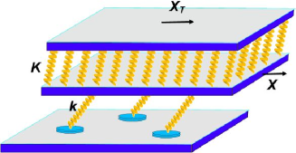
Figure 1: (Color online): The earthquake-like model. Friction occurs between the lower plate and the top block schematized by two plates connected by a network of springs to describe its internal shear stress. Thr contacts are represented by the disks on the lower plate and their elasticity is modeled by the springs connecting the lower plate and the bottom of the top block. The arrow indicate the displacement of the block. $X$ and $X_{T}$ are the coordinates of the bottom and top of the block.

The contacts may also interact elastically between themselves. As the top block moves, the surface stress at any contact increases, $f_{i}(t)=k_{i}x_{i}(t)$, where $x_{i}(t)$ is the shift of the $i$th junction from its non-stressed position. A single contact is assumed to be pinned whilst $f_{i}(t)<f_{si}$, where $f_{si}$ is the static friction threshold for the given contact. When the force reaches $f_{si}$, a rapid local slip takes place, during which the local stress in the block drops to the value $f_{bi}\approx 0$ while the elastic energy stored in the junction is released in the form of phonons into the bulk. Then the contact is pinned again, and the whole process repeats itself. Let $N_{c}$ be the number of contacts (asperities, bridges, etc.) at the interface. Each contact is characterized by its area $A_{i}$. The value of $k_{i}$, according to Persson P1995 , can be estimated as $k_{i}\sim\rho\,c^{2}\sqrt{A_{i}}$, where $\rho$ is the mass density and $c$ is the transverse sound velocity of the material which forms the contacts (see Appendix A). Let us assume that the substrates are rigid, i.e., the elastic constant of the substrate is infinite, $K=\infty$, and also neglect elastic interactions between the contacts through the substrate as it was done in the statistical studies of static friction GW1966 .

Let $P_{c}(x_{s})$ be the normalized probability distribution of values of the thresholds $x_{si}=f_{si}/k_{i}$ at which contacts break, where $f_{si}$ is the maximum force that contact $i$ can sustain. If we denote by $\bar{x}_{s}$ its average value and by $\sigma_{s}$ its standard deviation, a typical example is the Gaussian $P_{c}(x)=G(x;\bar{x}_{s},\sigma_{s})$, where

$$G(x;\bar{x},\sigma))=\frac{1}{\sigma\sqrt{2\pi}}\,\exp\left[-\frac{1}{2}\left(\frac{x-\bar{x}}{\sigma}\right)^{2}\right].$$ (1)

In numerics, the distribution $P_{c}(x)$ is defined on the interval $0<x<x_{m}$, where $x_{m}\gg\bar{x}_{s}$ so that we use the corrected distribution $P_{c}(x)={\cal N}\left\{P_{G}(x)-P_{G}(0)-(x/x_{m})\left[P_{G}(x_{m})-P_{G}(0)\right]\right\}$, where ${\cal N}$ is the normalization constant, so that $P_{c}(x)$ satisfies the condition $P_{c}(0)=P_{c}(x_{m})=0$.

To describe the kinetics of the model, we introduce the distribution $Q(x;X)$ of the stretchings $x_{i}$ when the top substrate is at a position $X$. It is normalized by

$$\int_{-\infty}^{\infty}dx\,Q(x;X)=1.$$ (2)

Let all contacts start from an initial distribution $Q(x;0)=Q_{\rm ini}(x)$ corresponding to the Gaussian one, $Q_{\rm ini}(x)=G(x;\bar{x}_{\rm ini},\sigma_{\rm ini})$ with $\bar{x}_{\rm ini}\ll\bar{x}_{s}$ and $\sigma_{\rm ini}\lesssim\sigma_{s}$. Let us now apply an adiabatically increasing force $F$ to the top substrate, while the bottom substrate remains fixed. The force will induce a displacement $X$ of the top substrate. According to third Newton’s law (the law of action and reaction), in the adiabatic regime of quasi-equilibrium $F$ must be compensated by the sum of elastic forces in the contacts,

$$F(X)=N_{c}\langle k_{i}\rangle\int_{-\infty}^{\infty}dx\,x\,Q(x;X)\,,$$ (3)

where we assumed that $k_{i}$ and $x_{i}$ are independent random variables.

With the increase of $F$ and consequently $X$, the stretching of a contact $i$ grows by the value $X$ with respect to its initial value, until it reaches the threshold stretching $x_{si}$ for the given contact. At this point the contact slides and $x_{i}$ drops; we assume that the sliding is rapid and that the stretching drops to zero, $x_{bi}=0$. In the numerical algorithm, the contact closest to the threshold is found and the displacement necessary to provoke a slip in this contact is added to all contacts. When the contact $i$ reaches the threshold and $x_{i}$ is set to zero, a new threshold is assigned to this contact randomly from the distribution $P_{c}(x)$. Then the whole process repeats itself.

Figure 2: (a) Short-time evolution of the EQ model. Solid curves show the distribution $Q(x;X)$ for incrementally increasing values of $X$ (with the step $\Delta X=0.05$). The distribution $P_{c}(x)$ is Gaussian with $\bar{x}_{s}=1$ and $\sigma_{s}=0.05$, the initial distribution $Q_{\rm ini}(x)$ is Gaussian with $\bar{x}_{\rm ini}=0$ and $\sigma_{\rm ini}=0.025$. For clarity each graph of $Q(x;X)$ is shifted by $0.025$ along the $x$ direction and by $-1$ along the $Q$ direction with respect to the previous one. (b) The corresponding dependence $F(X)$. The elastic constants are $\langle k_{i}\rangle=1$ and the top block is assumed to be fully rigid.

Figure 3: The same as in Fig. 2 for long times with the increment $\Delta X\approx 1.05$. While the initial distribution extended to negative $x$ values, according to the model this is not the case for further ones, which gives rise to what appears as a bump at $x$ = 0 (taking into account the shifts introduced for clarity).

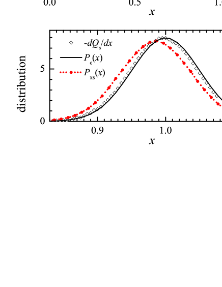
Figure 4: (Color online): The averaged final distribution $Q_{s}(x)$ for the parameters used in Figs. 2 and 3. The lower panel compares the functions $P_{c}(x)$ (solid line) and $-dQ_{s}(x)/dx$ (open diamonds). Red dotted curve and circles show the averaged final distribution of static thresholds.

The evolution of the system is shown in Fig. 2 for short times and in Fig. 3 for long times. One can see that, as time goes, the initial distribution approaches a stationary distribution $Q_{s}(x)$, where the total force $F$ becomes independent on $X$, and the final distribution (see Fig. 4) is independent of the initial one. An elegant mathematical proof of this statement for a simplified version of the EQ model was presented in Ref. FDW2005 ; the statement is valid for any distribution $P_{c}(x)$ except the singular case of $P_{c}(x)=\delta(x-x_{s})$.

Note that the probability distribution $P_{c}(x)$, which determines the value of the static threshold $x_{si}$ for newborn contacts is different from the concrete realization of the distribution of static thresholds $P_{xs}(x)$ (i.e., the histogram calculated over the array $\{x_{si}\}$). While at the beginning $P_{xs}(x)=P_{c}(x)$, then the function $P_{xs}(x)$ changes with time and finally takes the form shown in Fig. 4 (lower panel) by solid curve and circles. This is clearly demonstrated in Fig. 20 of Appendix B, where we consider a simple case of rectangularly-shaped function $P_{c}(x)$.

III Master equation approach

III.1 Master equation

Let us now introduce an analytical description of the evolution of the distribution $Q(x;X)$. When the top substrate is displaced by a small amount $\Delta\!X>0$ (the case of $\Delta\!X<0$ is considered in Appendix C), this increases all displacements of the contacts by $\Delta\!X$ too. This displacement leads to three kinds of changes in the distribution $Q(x;X)$: first, there is a global shift for all contacts, second, some contacts break because their stretchings become too large, and third, those broken contacts will form again, at a lower stretching after a slip at the scale of those contacts, which locally reduces the tension within the top substrate (or the tension of the corresponding springs in the spring-block model). These three contributions can be written as a master equation for $Q(x;X)$:

$$Q(x;X+\Delta\!X)=Q(x-\Delta\!X;X)-\Delta Q_{-}(x;X)+\Delta Q_{+}(x;X).$$ (4)

The first term in the r.h.s. of Eq. (4) is just the shift.

The second term $\Delta Q_{-}(x;X)$ designates the variation of the distribution due to the breaking of some contacts. We can formally write it as

$$\Delta Q_{-}(x;X)=P(x)\,\Delta\!X\,Q(x;X)\;,$$ (5)

where $P(x)\,\Delta\!X$ is the fraction of contacts displaced by $x$ from their fully relaxed state which break when their displacement is increased by $\Delta X$. This fraction is related to the individual properties of the contacts, which are determined by the distribution of static thresholds of each contact $P_{c}(x)$ defined in Sec. II. According to the definition of $P_{c}(x)$, the total number of unbroken contacts when the stretching of the asperities is equal to $x$ is given by $N_{c}\int_{x}^{\infty}P_{c}(\xi)\;d\xi$. The contacts that break when their displacements are increased by $\Delta\!X$ are those which have their thresholds between $x$ and $x+\Delta\!X$, i.e. $N_{c}P_{c}(X)\,\Delta\!X$. Therefore

$$P(x)=\frac{P_{c}(x)}{\int_{x}^{\infty}P_{c}(\xi)\;d\xi}\;.$$ (6)

The broken contacts relax and have to be added to the distribution around $x\sim 0$, leading to the third term in Eq. (4). We denote by $R(x)$ the normalized distribution of the stretching of the asperities that form a new contact after a slip event. Writing that all broken contacts described by $\Delta Q_{-}(x;X)$ immediately reappear with the distribution $R(x)$ (see Appendix D), we get

$$\Delta Q_{+}(x;X)=R(x)\int_{-\infty}^{\infty}dx^{\prime}\,\Delta Q_{-}(x^{\prime};X).$$ (7)

Equation (4) can be rewritten as

$$\left[Q(x;X+\Delta\!X)-Q(x;X)\right]+\left[Q(x;X)-Q(x-\Delta\!X;X)\right]$$

$$=-\Delta Q_{-}(x;X)+\Delta Q_{+}(x;X).$$

Taking the limit $\Delta\!X\to 0$, we finally get the integro-differential equation

$$\frac{\partial Q(x;X)}{\partial x}+\frac{\partial Q(x;X)}{\partial X}+P(x)\,Q(x;X)$$

$$=R(x)\int_{-\infty}^{\infty}dx^{\prime}\,P(x^{\prime})\,Q(x^{\prime};X),$$ (8)

which has to be solved with the initial condition

$$Q(x;0)=Q_{\rm ini}(x).$$ (9)

Note that $Q_{\rm ini}(x)$ cannot be an arbitrary function, because the contacts that exceed their stability threshold, must relax from the very beginning.

In the following we select $R(x)=\delta(x)$, i.e. we assume that a broken contact sticks again only after a complete relaxation. This is physically reasonable and simplifies the analytical calculations, although this restriction could be easily lifted for numerical solutions of Eq. (8).

Integrating both sides of Eq. (8) over $x$ from $-\infty$ to $\infty$, we see that the normalization condition (2) is satisfied, taking into account $Q(-\infty,X)=Q(+\infty,X)=0$ because contacts cannot be infinitely stretched without breaking.

Once the distribution $Q(x;X)$ is known, we can calculate the total force $F$ with Eq. (3) and find the static friction force as the maximum of $F(X)$, i.e., $F_{s}=F(X_{s})$, where $X_{s}$ is a solution of the equation

$$F^{\prime}(X)\equiv dF(X)/dX=0.$$ (10)

III.2 Steady state solution

The smooth-sliding solution $Q_{s}(x)$, i.e. the solution which does not depend on $X$, can easily be found directly P1995 . In the steady state Eq. (8) reduces to

$$\frac{dQ(x)}{dx}+P(x)\,Q(x)=\delta(x)\int_{0}^{\infty}dx^{\prime}\,P(x^{\prime})\,Q(x^{\prime}).$$ (11)

In setting the lower bound of the integral we have assumed that $P_{c}(x)=0$ for $x\leq 0$, which agrees with its physical meaning because, if $x<0$, a positive variation $\Delta X$ actually reduces the absolute value of the force on a contact so that it does not cause its breaking.

Its general solution can easily be derived for $x>0$ and leads to

$$Q_{s}(x)=C^{-1}\Theta(x)E_{P}(x),$$ (12)

where $\Theta(x)$ is the Heaviside step function, $\Theta(x)=0$ for $x<0$ and $\Theta(x)=1$ for $x\geq 0$,

$$E_{P}(x)=e^{-U(x)},\;\;\;U(x)=\int_{0}^{x}d\xi\,P(\xi)\;,$$ (13)

and this solution also verifies the equation in the limit $x\to 0$. The normalization condition for $Q_{s}(x)$ gives

$$C=\int_{0}^{\infty}dx\,E_{P}(x).$$ (14)

The friction force is then equal to

$$F=(N_{c}\langle k_{i}\rangle/C)\int_{0}^{\infty}dx\,xE_{P}(x).$$ (15)

Two simple examples are considered in Appendix B.

III.3 Relation between the EQ and ME

The EQ model is expressed in terms of the distribution of breaking thresholds of the contacts $P_{c}(x)$. Therefore, to connect the two approaches it is interesting to relate the steady state solution of the ME equation and the function $P_{c}(x)$. Using Eq. (6) we get

$$Q_{s}(x)=C^{-1}\Theta(x)\exp\left[-\int_{0}^{x}d\xi\,\frac{P_{c}(\xi)}{\int_{\xi}^{\infty}P_{c}(\xi^{\prime})\;d\xi^{\prime}}\right]\;.$$ (16)

The integration in the exponential can be readily performed since the integrand is of the form $(d/d\xi)\ln\int_{\xi}^{\infty}P_{c}(\xi^{\prime})\,d\xi^{\prime}$. We get

$$Q_{s}(x)=C^{-1}\Theta(x)\int_{x}^{\infty}P_{c}(\xi)\;d\xi,$$ (17)

or ($x>0$)

$$\frac{dQ_{s}(x)}{dx}=-C^{-1}P_{c}(x)$$ (18)

in agreement with the observations deduced from the numerical simulations of the EQ model (Fig. 4, lower panel). For the parameters used in Figs. 2–4, the numerical constant is $C=0.9999$.

Notice also the useful relationships $U^{\prime}(x)=P(x)$, $E_{P}^{\prime}(x)=-E_{P}(x)P(x)$, $E_{P}(x)=1$ for $x\leq 0$, and

$$P_{c}(x)=P(x)\,E_{P}(x)\;\;\;{\rm for}\;\;\;x>0,$$ (19)

the latter may be used in numerical solution of the ME instead of Eq. (6).

For the simple example of a rectangular $P_{c}(x)$ distribution, which is considered in Appendix B, the model admits an exact solution both for the EQ and ME approaches. We checked that the earthquake model with the distribution (63) and the master equation model with the expression (64) for $P(x)$ exactly have the same solution for any initial configuration.

III.4 Non-stationary solution

The numerical solution of the master equation (8) when $X$ starts to grow due to an external driving is presented in Figs. 5 and 6 for a Gaussian distribution of static contact thresholds, $P_{c}(x)=G(x;\bar{x}_{s},\sigma_{s})$.

Figure 5: (a) Solution of the master equation in the initial stage when $X$ starts to grow. The model parameters are the same as in Fig. 2. (b) The corresponding dependence $F(X)$.

Figure 6: The same as in Fig. 5 for long times with the increment $\Delta X=1.09$.

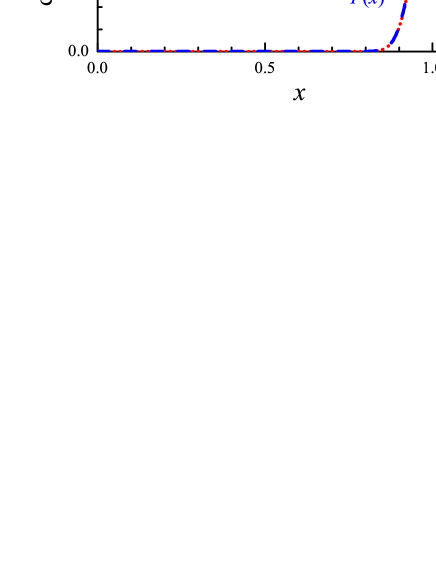
Figure 7: (Color online): The final distribution $Q(x)$ for the parameters used in Fig. 6 (solid curve; crosses show the averaged final distribution for the earthquake model from Fig. 4). The red dotted curve shows the distribution $P_{c}(x)$, blue broken curve – the function $P(x)$.

This solution may be compared with that of the EQ model of Figs. 2 and 3 for the same initial condition. One can see that they are almost identical, except for the noise on the earthquake model distributions. The distribution $Q(x;X)$ always approaches the stationary distribution $Q_{s}(x)$ given by Eq. (12). The final distributions of the EQ model and the ME approach are compared in Fig. 7.

Let the distribution $P_{c}(x)$ be characterized by the average value $\bar{x}_{s}$ and the dispersion $\sigma_{s}$. Studying the evolution presented in Fig. 5, we observe that every-time $X$ increases by $\bar{x}_{s}$ the distribution $Q(x;X)$ broadens so that its standard deviation grows by $\sim\sigma_{s}$. Therefore, any initially peaked distribution tends to approach the stationary one according to $|Q(x;X)-Q_{s}(x)|\propto\exp(-X/X^{*})$, where $X^{*}\sim\bar{x}_{s}^{2}/\sigma_{s}$.

For one particular but important choice of the initial distribution, when all contacts are relaxed at the beginning, $Q_{\rm ini}(x)=\delta(x)$, one can analytically express the initial evolution of the solution versus $X$. Namely, if $P(x)=0$ for the stretchings $x<x_{c}^{*}$, then, as can be checked by its substitution in the master equation, the solution for the displacement $X<2x_{c}^{*}$ is the following: at the beginning, for the displacement $0<X<x_{c}^{*}$, the solution is trivial, $Q(x;X)=\delta(x-X)$ and $F(X)=N_{c}\langle k_{i}\rangle X$; for larger displacements, $x_{c}^{*}<X<2x_{c}^{*}$, the solution is

$$Q(x;X)=\left\{\begin{array}[]{ll}\Theta(x)\,b(X-x)&{\rm for}\;\;\;0\leq x<X-x_{c}^{*},\\ 0&{\rm for}\;\;\;X-x_{c}^{*}\leq x<x_{c}^{*},\\ a(X)\,\delta(X-x)&{\rm for}\;\;\;x\geq x_{c}^{*},\end{array}\right.$$ (20)

where

$$b(\xi)=P(\xi)\,a(\xi)$$ (21)

and $a^{\prime}(\xi)=-P(\xi)a(\xi)$, or

$$a(\zeta)=\exp\left[-\int_{x_{c}^{*}}^{\zeta}d\xi\,P(\xi)\right],\;\;\;\zeta\geq x_{c}^{*}.$$ (22)

Then one can calculate the friction force for the displacement interval $x_{c}^{*}<X<2x_{c}^{*}$

$$F(X)=N_{c}\langle k_{i}\rangle\left[Xa(X)+(X-x_{c}^{*})-\int_{x_{c}^{*}}^{X}d\xi\,a(\xi)\right].$$ (23)

The solution (23) allows us to find the static friction force $F_{s}=F(X_{s})$ with Eq. (10), which reduces to the equation $X_{s}a(X_{s})P(X_{s})=1$ and corresponds to the first maximum on the variation of $F(X)$. As was pointed out by Farkas et al. FDW2005 , the ratio $F_{s}/F_{k}$, where $F_{k}$ is the kinetic friction, i.e. the plateau reached by $F(X)$, takes values between 1 and 2 [larger values corresponding to narrower distributions $P_{c}(x)$], and it is determined solely by the initial distribution $Q_{\rm ini}(x)$, reaching a maximum for $Q_{\rm ini}(x)=\delta(x)$ (it was called “the initial coherence in strain distribution of the contacts” in Ref. FDW2005 ).

Thus, in a general case, as $X$ grows the solution of the master equation always approaches the smooth-sliding state given by Eqs. (12–14). However, there is one exception to this general scenario, when the model admits a periodic solution. This is the singular case when all contacts are identical, i.e., all contacts are characterized by the same static threshold $x_{s}$, so that $P_{c}(x)=\delta(x-x_{s})$. The steady-state solution of Eq. (8) for this case is described in Appendix E. We emphasize that the solution (20) is valid for the continuous distribution $P_{c}(x)$ only, it cannot be used for the singular $P_{c}(x)=\delta(x-x_{s})$ case.

III.5 Nonrigid substrates: stick-slip

The master equation allows us to compute the friction force $F(X)$ when the bottom of the sliding block is displaced by $X$. But actually in an experiment one does not control $X$. The displacement is caused by a shearing force $F_{T}$ applied to the top of the sliding block, which displaces its top surface by $X_{T}$. As the strain on the sliding block is usually small, its deformation can be assumed to be elastic, so that $X_{T}$ is related to the applied force by

$$F_{T}=K(X_{T}-X),$$ (24)

where $K$ is the shear elastic constant of the solid block. The solution that we discussed above amounts to assuming that the sliding block was infinitely rigid, $K\to\infty$, so that $X_{T}=X$ at any time. In this case we found that the sliding always tends to a smooth-sliding steady state, as expected for a stiff system P0 ; BC2006 ; BN2006 . Let us now consider the case of finite $K<\infty$. The total force applied to the bottom of the sliding block, which determines its displacement $X$, is the sum of the applied force and the friction force

$$F_{\mathrm{tot}}=K(X_{T}-X)-F(X)\;.$$ (25)

It can be viewed as derived from the potential

$$V(X_{T},X)=\frac{1}{2}K(X_{T}-X)^{2}+\int_{0}^{X}F(\xi)\,d\xi\;,$$ (26)

which determines the behavior of the sliding block subjected to friction and the applied force.

A necessary condition for smooth sliding is that $X_{T}$ and $X$ grow together, with $X_{T}-X=B$, where $B$ is a constant that measures the shear strain in the sliding block. This leads to the condition

$$\frac{\partial V}{\partial(X_{T}-X)}=\frac{\partial V}{\partial X}=0\;,$$ (27)

which simply means that the total force on the sliding interface vanishes. Smooth sliding also requires this state to be stable

$$\frac{\partial^{2}V}{\partial(X_{T}-X)^{2}}=\frac{\partial^{2}V}{\partial X^{2}}\geq 0\quad\mathrm{or} \quad F^{\prime}(X)\geq-K\;.$$ (28)

These arguments exactly coincide with the “elastic instability” widely discussed in literature (e.g., see Ref. BC2006 and references therein).

If we start from relaxed asperities, in the early stage of the motion $F(X)$ is a growing function of $X$, and then it passes by a maximum when some contacts start to break and reform at lower asperity stress. Depending on the value of $K$, two situations are possible. For large $K$ (stiff block), $F^{\prime}(X)$ never falls below $-K$ and the smooth sliding is a stable steady state. In this case the system evolves towards the regime $F(X)=$ Const defined by Eq. (15). For small $K$ (soft block), $F^{\prime}(X)$ can become smaller than $-K$ and the stability condition (28) is no longer valid. In this case Eq. (28), in the the limiting case of the equality, defines the maximal displacement $X_{m}$ that the contacts can sustain. A larger displacement breaks all the contacts simultaneously, causing a quick slip of the block before the contacts form again with a fresh distribution $Q(x,X_{m})=R(x)$ and the same process can repeat again. The system may reach the regime of stick-slip periodic motion BT2009 . Using the solution (23) for the delta-function initial distribution, we get $F^{\prime}(X)=N_{c}\langle k_{i}\rangle\left[1-XP(X)\,a(X)\right]$, so that we can find the period $X_{ss}$ of the stick-slip motion with Eq. (28). Ignoring the slip time, it is given by the solution of the equation $X\,a(X)P(X)=1+K/N_{c}\langle k_{i}\rangle$ for $X>x_{c}^{*}$. Note that in the case of an extremely soft substrate, $K\to 0$, the motion (almost always) corresponds to stick-slip, as it should for such a soft system P0 ; BC2006 ; BN2006 .

Thus, depending on the distribution $P_{c}(x)$, the system demonstrates either stick-slip or smooth sliding. Smooth sliding is achieved if $K>K^{*}$, otherwise the elastic instability occurs which may result in stick-slip. As $K^{*}=\max[-F^{\prime}(X)]$ and $F(X)$ reaches its maximum for $X\simeq\bar{x}_{s}$, one can estimate that $K^{*}\sim N_{c}\langle k\rangle\,\bar{x}_{s}/\sigma_{s}$; thus, the ratio $\sigma_{s}/\bar{x}_{s}$ controls the appearance of the elastic instability.

IV Temperature effects

The effect of a nonzero temperature is connected with a change of the fraction density of breaking contacts $P(x)$ in the master equation (8) as first discussed by Persson P1995 . Indeed, for a single contact with the static threshold $x_{s}$ at zero temperature, the contact does not break at all for $x<x_{s}$. But when $T>0$, the contact may relax due to a thermally activated jump before the threshold $x_{s}$ is reached. The rate $h(x;x_{s})$ of this process is defined by

$$dQ(t)/dt=h(x;x_{s})\,Q(t),\;\;\;x<x_{s}\;,$$ (29)

where $Q(t)$ is the probability that a contact existing at $t=0$ is not thermally broken at time $t$. For a set of contacts, Eq. (29) has to be generalized to

$$dQ(t)/dt=H(x)\,Q(t)$$ (30)

with

$$H(x)=\int_{x}^{\infty}dx^{\prime}\,h(x;x^{\prime})\,P_{c}(x^{\prime}).$$ (31)

For a sliding at velocity $v$ so that $X=vt$, the thermally activated jumps can be incorporated in the master equation, if we use a corrected expression $P_{T}(x)$ defined by

$$P_{T}(x)=P(x)+H(x)/v\;,$$ (32)

instead of the zero-temperature breaking fraction density $P(x)$.

The rate of thermal activation of the contacts, $h(x;x_{s})$ in Eq. (29), can be estimated by the Kramers relation. Let $V(x)$ be the binding energy of the contact, and $\Delta E(x;x_{s})=V(x_{s})-V(x)$, the activation energy for the contact to break. For “soft”, or “weak” contacts, when $\Delta E(0;x_{s})\gtrsim k_{B}T$, the rate $h(x;x_{s})$ is given by P1995 ; FKU2004

$$h(x;x_{s})\approx\omega\,\exp\left[-\Delta E(x;x_{s})/k_{B}T\right],$$ (33)

where $\omega$ is a prefactor corresponding to the attempt frequency. For an overdamped dynamics of the contacts $\omega\approx\omega_{0}^{2}/2\pi\eta$ with the characteristic frequency $\omega_{0}^{2}\sim k/m\sim c^{2}/A$ ($m$ is the contact mass) and the damping coefficient $\eta\sim c/\sqrt{A}$ which gives $\omega\sim c/2\pi\sqrt{A}\sim 10^{10}$ s^-1 P1995 . If we assume that the binding potential of a contact can be approximated by the elastic properties of this contact, then $V(x)={1\over 2}\,kx^{2}$. In this case the activation energy for contact breaking takes the form P1995

$$\Delta E(x;x_{s})={1\over 2}\,k(x_{s}^{2}-x^{2})\approx kx_{s}\,(x_{s}-x),$$ (34)

and the function $H(x)$ in Eq. (32) is given by

$$H(x)=\omega\,e^{kx^{2}/2k_{B}T}\int_{x}^{\infty}d\xi\,P_{c}(\xi)\,e^{-k\xi^{2}/2k_{B}T}.$$ (35)

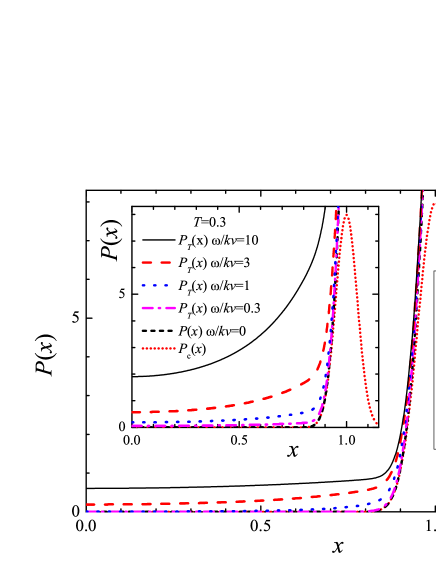
Figure 8: (Color online): The rate $P_{T}(x)$ for soft contacts at different temperatures $T=0$ (black short dashed), 0.03 (magenta dash-dotted), 0.1 (blue dotted), 0.3 (red dashed) and 1 (black solid curve) for a given velocity, $\omega/kv=1$. Inset: the rate $P_{T}(x)$ at different velocities $\omega/kv=0$ (black short dashed), 0.3 (magenta dash-dotted), 1 (blue dotted), 3 (red dashed) and 10 (black solid curve) for a fixed temperature $T=0.3$. The red short-dotted curve shows the distribution $P_{c}(x)$ (Gaussian with $\bar{x}_{s}=1$ and $\sigma_{s}=0.05$).

For “stiff”, or “strong” contacts, when $\Delta E(0;x_{s})\gg k_{B}T$, contact breaking only occurs with a significant probability when the stretching $x$ of a contact is close to the threshold $x_{s}$. The harmonic expression of the binding energy can no longer be used and a cubic approximation is more appropriate. This leads to a correction in the activation energy Garg1995 ; Dudko2003

$$\Delta E(x;x_{s})=\Delta E(0;x_{s})\left(1-x/x_{s}\right)^{3/2},$$ (36)

and a renormalization of the prefactor $\omega$,

$$\omega\to\omega\,\left(1-x/x_{s}\right)^{1/2},$$ (37)

so that the function $H(x)$ is given by

$$H(x)=\omega\,\int_{x}^{\infty}d\xi\,P_{c}(\xi)\left(1-\frac{x}{\xi}\right)^{\frac{1}{2}}\exp\left[-\frac{k\xi^{2}(1-x/\xi)^{\frac{3}{2}}}{2k_{B}T}\right].$$ (38)

The contributions (35) or (38) to the rate $P_{T}(x)$ lead to appearance of a low-$x$ tail. Its magnitude grows with temperature as well as with a decrease of the driving velocity $v$ as demonstrated in Fig. 8.

Raising temperature leads to a shift of the distribution $Q(x)$ to lower values, so that the friction force decreases when $T$ grows. This effect is larger for lower sliding velocities as shown in Fig. 9. In the limit $v\to 0$, all contacts finally break if $T\neq 0$, so that $Q_{s}(x)\to\delta(x)$ and $F_{k}\to 0$; in this limit we have a smooth sliding associated to a creep motion of the contacts.

Figure 9: (Color online): The steady-state distribution $Q_{s}(x)$ for $T=0.3$ and different velocities $\omega/kv=0.3$ (magenta dash-dotted), 1 (blue dashed), 3 (red short-dotted) and 10 (black solid curve) for the soft contacts. The distribution $P_{c}(x)$ is Gaussian with $\bar{x}_{s}=1$ and $\sigma_{s}=0.05$.

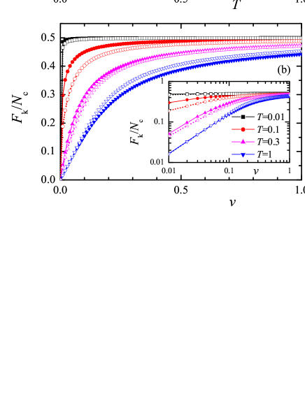
Figure 10: (Color online): (a) Dependence of the kinetic friction force $F_{k}$ in the steady state on the temperature $T$ for different velocities $v=0.01$ (black squares), 0.1 (red circles), 1 (magenta up triangles) and 10 (blue down triangles). (b) $F_{k}(v)$ for different temperatures $T=0.01$ (black squares), 0.1 (red circles), 0.3 (magenta up triangles) and 1 (blue down triangles); the inset shows the same in log-log scale. Solid curves and symbols are for soft contacts, and broken curves and open symbols, for stiff contacts. The distribution $P_{c}(x)$ is Gaussian with $\bar{x}_{s}=1$ and $\sigma_{s}=0.05$; $\omega/k=1$.

The variation of $F_{k}(T)$ versus $T$ for different sliding velocities in the smooth sliding regime for soft and stiff contacts is presented in Fig. 10a. As expected, the friction force decreases when $T$ grows and tends to zero when $T\to\infty$. Figure 10b shows the dependence of kinetic friction on the sliding velocity. The force $F_{k}$ monotonically increases with $v$, approaching the $T=0$ limit when $v\to\infty$. The dependence $F_{k}(v)$ at smooth sliding was estimated analytically by Persson P1995 (see also Ref. SW2009 ) who found $F_{k}(v)\propto v$ in the low-velocity limit, $F_{k}(v)\propto\ln v$ for intermediate velocities, and $F_{k}(v)-F(\infty)\propto-\omega T^{2}/kv$ in the high-velocity case.

Thus, for $T>0$ the friction force $F_{k}$ increases with the driving velocity, i.e. $dF_{k}(v)/dv>0$, which stabilizes the smooth sliding regime. However, experiments show that the temperature-induced velocity-strengthening only dominates the aging-induced velocity-softening (see Sec. V) at high velocities $v>10-100$ $\mu$m/s BC2006 .

Of course, a nonzero temperature also affects the dynamics of the approach to the steady state as shown in Fig. 11 for different driving velocities. The higher the temperature and/or the lower the velocity are, the lower is the static friction force $F_{s}$ [determined by the first maximum of the $F(X)$ dependence], and the faster $F(X)$ approaches the steady-state smooth sliding. It is important to consider the first cycle of the $F(X)$ dependence, which defines the lowest value of $F^{\prime}(X)$ because it determines the stability limit of the smooth sliding regime according to Eq. (28). As shown in Fig. 12, higher temperatures (Fig. 12a) raise the minimum value of $F^{\prime}(X)$, which in turn extends the interval of the model parameters for which the smooth sliding takes place. At the same time, the higher is driving velocity (Fig. 12b), the smaller is the minimum of $F^{\prime}(X)$, so that the narrower is the interval of model parameters where the smooth sliding regime exists. Thus, we come to a surprising conclusion that, at $T>0$, reducing the pulling velocity may lead to a transition from stick-slip to smooth sliding or creep motion, while one generally expects that smooth sliding is reached when the velocity increases. However a transition to smooth motion by reducing velocity has also been observed experimentally YGI1993 .

Figure 11: The dependences $F(X)$ for $T=0.3$ at different driving velocities $v$, $\omega/kv=0$, 0.3, 1, 3 and 10. The distribution $P_{c}(x)$ is Gaussian with $\bar{x}_{s}=1$ and $\sigma_{s}=0.05$, the initial distribution $Q_{\rm ini}(x)$ is Gaussian with $\bar{x}_{\rm ini}=0.1$ and $\sigma_{\rm ini}=0.025$.

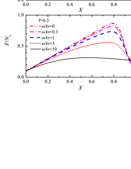
Figure 12: (Color online): The same as in Fig. 11 for short $X$. (a) is for different temperatures $T=0$ (red dash-dot-dotted), 0.03 (magenta dash-dotted), 0.1 (blue dashed), 0.3 (red dotted) and 1 (black solid curve) at the fixed velocity, $\omega/kv=1$; (b) is for different velocities $v$, $\omega/kv=0$ (red dash-dot-dotted), 0.3 (magenta dash-dotted), 1 (blue dashed), 3 (red dotted) and 10 (black solid curve) at the fixed temperature $T=0.3$.

The behavior of $F_{k}$ on $T$ and $v$ described above is only qualitative. A quantitative study to identify the temperature range in which these effects would play a significant role in an actual material would require a specific study. However it qualitatively agrees with tip-based experiments SO2003 ; SJHF2006 , which suggest that, in these experiments, the tip/substrate contact occurs through many atoms, i.e. it actually corresponds to multiple contacts. Surprisingly, the dependences obtained within the ME approach, perfectly agree with the experimental ones for a model tribological system MIKOT2005 ; MIKSOTN2005 ; MN2007 ; NKKGMKB2007 , where the wearless kinetic friction of the driven lattice of quantized magnetic vortexes in high-temperature cuprate superconductors was studied (e.g., compare inset of Fig. 10b with Fig. 3 of Ref. MIKOT2005 ).

However our approach only claims to explain the general trends of the behavior of tribological systems, because we neglected several important factors. First, we neglected contact aging (see Sec. V). Second, we assumed that $R(x)=\delta(x)$, while at $T>0$ the distribution $R(x)$ of stretchings when contact form again after a slip event should correspond to the Boltzmann distribution around $x=0$ with a width depending on $T$ FKU2004 ; SW2009 . Third, in a real system the contacts are heated due to sliding and even may change their structure. Forth, we ignored the elastic interaction between the contacts. Finally, in macroscopic experiments the wearing of substrates in sliding contact may mask the temperature and velocity dependences. A more detailed investigation of these aspects deserves separate studies.

V Aging of the contacts

In the approach described in Sec. III, the function $F(X)$ was independent on the driving velocity because we neglected two time-dependent effects: first a broken contact needs a minimum delay $\tau_{m}$ to stick again, second we ignored the aging of the contacts once they are formed, which contradicts most of the experimental results P0 ; BN2006 ; BC2006 . Experiments as well as molecular dynamics simulations indicate that the static friction force grows with the lifetime $t_{w}$ of stationary contacts, i.e. the time interval during which they stay static prior to sliding.

The simplest way to obtain a velocity dependence of the function $F(X)$ is to take into account the delay time $\tau_{m}$. This is considered in Appendix D. In the most general case the delay time may not be the same for all contacts but exhibits some distribution. In Ref. BT2009 we showed that the condition $\tau_{m}>0$ is the second necessary condition for the appearance of stick-slip.

Let us now consider the aging of contacts which requires a more involved analysis because we must take into account a time evolution of the distribution $P_{c}(x)$ of the contact breaking thresholds. Let the newborn contacts be characterized by a distribution $P_{ci}(x)$ with the average value $\bar{x}_{si}$ and the dispersion $\sigma_{si}$. If aging effects are taken into account, then typically $\bar{x}_{s}$ grows with time, while $\sigma_{s}$ decreases, because the area of contact slowly grows under pressure. As it does it faster for the small contacts, which are less resilient, this tends to reduce the dispersion in the properties of the contacts. As a result, at $t\to\infty$ the distribution $P_{c}(x)$ approaches a distribution $P_{cf}(x)$ with $\bar{x}_{sf}>\bar{x}_{si}$ and $\sigma_{sf}<\sigma_{si}$. The final distribution is a property of the material. It is therefore a known quantity for the model once the material has been specified. If we assume that the evolution of $P_{c}(x)$ corresponds to a stochastic process, then it should be described by a Smoluchowsky equation

$$\frac{\partial P_{c}}{\partial t}=D\,\widehat{L}_{x}P_{c},\;\;\;{\rm where}\;\;\;\widehat{L}_{x}\equiv\frac{\partial}{\partial x}\left(B(x)+\frac{\partial}{\partial x}\right),$$ (39)

in which the “diffusion” parameter $D$ describes the rate of aging, $B(x)=d\widetilde{U}(x)/dx$, and the “potential” $\widetilde{U}(x)$ defines the final distribution, $P_{cf}(x)\propto\exp\left[-\widetilde{U}(x)\right]$; therefore we can write

$$B(x)=-\frac{dP_{cf}(x)/dx}{P_{cf}(x)}.$$ (40)

Then, the equation $\partial P_{c}/\partial t=D\,\widehat{L}_{x}P_{c}$ naturally leads to a growth of the average static threshold from $\bar{x}_{si}$ to $\bar{x}_{sf}$ with the time of stationary contact, as widely assumed in earthquake-like models of friction BN2006 ; P1995 ; BR2002 . A characteristic timescale of aging may be estimated as $\tau_{\rm aging}=(\bar{x}_{sf}-\bar{x}_{si})^{2}/D$.

Figure 13: Evolution of $P_{c}(x)$ due to two concurrent processes: the first process is the aging of asperities from the initial (fresh) distribution $P_{ci}(x)$ (Gaussian with $\bar{x}_{si}=0.5$ and $\sigma_{si}=0.05$) to the final distribution $P_{cf}(x)$ (Gaussian with $\bar{x}_{sf}=1$ and $\sigma_{sf}=0.02$), and the second one is the breaking/re-binding of the contacts. $D_{X}\equiv D/v=5\times 10^{-4}$, the initial distribution $Q_{\rm ini}(x)$ is Gaussian with $\bar{x}_{\rm ini}=0.1$ and $\sigma_{\rm ini}=0.025$. The curves are plotted with the increment $\Delta X=0.05$.

At the same time, the contacts continuously break and form again when the substrate moves, as described by third and forth terms in Eq. (8). This introduces two extra contributions in the equation determining $\partial P_{c}(x;X)/\partial X$ in addition to the pure aging effect described by Eq. (39): a term $P(x;X)\,Q(x;X)$ takes into account the contacts that break, while their reappearance with the threshold distribution $P_{ci}(x)$ gives rise to the second extra term in the equation. Combining the equation describing the evolution of the distribution $Q(x;X)$ with the equation describing the aging of the contact properties, and taking into account the relation (19), we come to the system of three equations:

$$\frac{\partial Q(x;X)}{\partial x}+\frac{\partial Q(x;X)}{\partial X}+P(x;X)\,Q(x;X)$$

$$\;\;\;\;\;\;\;=\delta(x)\int_{-\infty}^{\infty}dx^{\prime}\,P(x^{\prime};X)\,Q(x^{\prime};X),$$

$$\frac{\partial P_{c}(x;X)}{\partial X}-D_{X}\widehat{L}_{x}P_{c}(x;X)+P(x;X)\,Q(x;X)$$

$$\;\;\;\;\;\;\;=P_{ci}(x)\int_{-\infty}^{\infty}dx^{\prime}\,P(x^{\prime};X)\,Q(x^{\prime};X),$$

$$P_{c}(x;X)=P(x;X)\,\exp\left[-\int_{0}^{x}d\xi\,P(\xi;X)\right],$$ (41)

where $D_{X}=D/v$, and $v=dX(t)/dt$ is the driving velocity. Thus, in the case of high driving ($v\to\infty$, $D_{X}\to 0$) we recover the previous behavior with $P_{c}(x)=P_{ci}(x)$. In the case of low driving ($v\to 0$, $D_{X}\to\infty$) we again observe the same type of behavior but with $P_{c}(x)=P_{cf}(x)$, and in the case of $0<D_{X}<\infty$ we have an interplay of two processes, the aging which tends to change $P_{c}(x)$ towards $P_{cf}(x)$, and the breaking-reformation of the contacts which returns $P_{c}(x)$ to $P_{ci}(x)$. This is illustrated in Fig. 13, where we plot the evolution of $P_{c}(x)$ when $X$ continuously increases. As a result, the friction force $F$ has to depend on the sliding velocity as shown in inset of Fig. 14b.

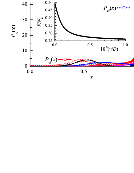
Figure 14: (Color online): (a) The final distribution $Q_{s}(x)$ for five values of the parameter $D_{X}=D/v$: $10^{-5}$ (black circles), $10^{-4}$ (blue up triangles), $3\times 10^{-4}$ (red crosses), $10^{-3}$ (magenta down triangles), and $10^{-2}$ (black diamonds). (b) The corresponding distributions $P_{c}(x)$. Larger open circles show the initial distribution $P_{ci}(x)$ (red dashed) and the final distribution $P_{cf}(x)$ (blue dotted). The inset displays the dependence of the kinetic friction force $F_{k}$ in the steady state on the driving velocity $v$ ($\langle k_{i}\rangle=1$). $P_{ci}(x)$ is Gaussian with $\bar{x}_{si}=0.5$ and $\sigma_{si}=0.1$, and $P_{cf}(x)$ is Gaussian with $\bar{x}_{sf}=1$ and $\sigma_{sf}=0.01$.

Because typically $\bar{x}_{si}<\bar{x}_{sf}$, the kinetic friction force $F_{k}$ generally decreases when $v$ grows, so that $dF_{k}(v)/dv<0$, which may lead to an instability of the smooth sliding regime.

The steady-state solution of Eqs. (41) can be found analytically in the low- and high-velocity cases. In the $v\to 0$ limit,

$$P_{c}(x)\approx P_{cf}(x)+\frac{v}{D}\frac{P_{cf}(x)}{C[P_{f}]}\times$$

$$\int_{0}^{x}d\xi\;P_{cf}^{-1}(\xi)\int_{0}^{\xi}d\xi^{\prime}\;\left[P_{cf}(\xi^{\prime})-P_{ci}(\xi^{\prime})\right],$$

which leads to $F_{k}(v)-F_{k}(0)\propto-v/D$, while in the high-velocity case, $v\to\infty$, we have

$$P_{c}(x)\approx P_{ci}(x)+\frac{D}{v}\;C[P_{i}]\frac{d}{dx}\left[B(x)+\frac{d}{dx}\right]P_{ci}(x),$$

which gives $F_{k}(v)-F_{k}(\infty)\propto D/v$. In these expressions $C[P]$ designates the constant $C$ defined by Eq. (14), which takes different values depending on the expression of $P(x)$. Both limiting cases may be combined within one fitting formula,

$$F_{k}(v)\approx F_{k}(\infty)+\frac{F_{k}(0)-F_{k}(\infty)}{1+v/v_{\rm aging}},$$ (42)

where $v_{\rm aging}$ defines the velocity below which aging effects become essential. For example, for the parameters used in Fig. 14 we found that $v_{\rm aging}\approx 6.5\times 10^{3}D$.

Figure 15: The dependences $F(X)$ for two driving velocities $v=1.5$ (a) and $v=1.6$ (b). The initial (fresh) distribution of thresholds $P_{ci}(x)$ is Gaussian with $\bar{x}_{si}=0.5$ and $\sigma_{si}=0.05$, the final distribution $P_{cf}(x)$ is Gaussian with $\bar{x}_{sf}=1$ and $\sigma_{sf}=0.02$. The initial distribution for contacts $Q_{\rm ini}(x)$ is Gaussian with $\bar{x}_{\rm ini}=0.02$ and $\sigma_{\rm ini}=0.01$ (for calculation reasons, the same is used for the “refreshed” distribution after the break at the point $F^{\prime}(X)=-K$). The parameters are $\langle k_{i}\rangle=1$, $K=3.5N_{c}\langle k_{i}\rangle$, and the rate of aging is determined by the coefficient $D_{X}=D/v$ with $D=5\times 10^{-4}$.

When the sliding substrates are not rigid, the effect of contacts aging may lead to a transition from stick-slip to smooth sliding with the increase of the sliding velocity. When the driving velocity increases and reaches a critical value $v=v_{c}$ the transition is abrupt (first-order) as demonstrated in Fig. 15. Moreover, the system exhibits hysteresis: starting from the smooth-sliding regime, if the velocity decreases we expect a smooth sliding to survive down to velocities much lower than $v_{c}$.

In a general case, the parameter $D$ in Eq. (41) and, therefore the rate of contacts aging, depends on the system temperature $T$. Typically, the aging rate should increase with $T$ according to Arrhenius law, $D\propto\exp\left(-\varepsilon/k_{B}T\right)$, where $\varepsilon$ is an activation energy for this process. Besides, aging mechanisms may be much more involved than the simplest one described by the Smoluchowsky equation (39) and may even consist of two stages BC2006 , the “geometrical” growth of contacts (described, e.g., by the Lifshitz-Slözov theory, see Sec. VI.5) and then a structural reordering of asperities.

VI Origin of threshold distribution

As discussed in the introduction the formalism using the master equation to describe friction allows us to separate the calculation of the friction force, assuming that the statistical properties of the contacts are known, from the analysis of the properties of the contact themselves. In the previous sections we focused on the calculation of the friction force, which is our main goal. However it is interesting to examine the properties of the contacts because it allows us to draw some general conclusions on friction, particularly on the possible existence of stick-slip. Within our approach the properties of the contacts are entirely described within the distribution $P_{c}(x)$ of the contact thresholds, which may be time dependent as discussed in Sec. V on aging. Let us now discuss possible physical origins of this distribution.

To establish the master equation, it is convenient to express the properties of the contacts in term of their stretching $x$, hence $P_{c}(x)$, but at the microscopic scale contacts are generally characterized by their breaking force. The distribution $P_{c}(x)$ can be related to the distribution $\widetilde{P}_{c}(f_{s})$ of the static friction force thresholds of the contacts. If a given contact has an area $A$, then it is characterized by the static friction threshold $f_{s}\propto A$ and the elastic constant $k\sim\rho\,c^{2}\sqrt{A}$, where $\rho$ is the mass density and $c$ the sound velocity (assuming that the linear size of the contact and its height are of the same order of magnitude P1995 ). The displacement threshold for the given contact is $x_{s}=f_{s}/k$, so that

$$f_{s}\propto x_{s}^{2},$$ (43)

or $df_{s}/dx_{s}\propto x_{s}$. Then, using the relationship $P_{c}(x_{s})\,dx_{s}=\widetilde{P}_{c}(f_{s})\,df_{s}$, we obtain

$$P_{c}(x_{s})\propto x_{s}\widetilde{P}_{c}[f_{s}(x_{s})].$$ (44)

VI.1 Rough surfaces: the GW model

Let us consider the contact of two nominally flat surfaces, for which the appararent contact area is large so that individual contacts are dispersed and the forces acting through neighboring spots do not influence each other GW1966 . Their study can be cast into the problem of the contact of a rigid plane and a composite surface whose topography is the sum of both topographies, with an appropriate renormalization of some parameters such as the Young modulus, so that the contact problem reduces to the statistics of independent asperities BC2006 . Let the rough surface be characterized by hills of heights $\{h_{i}\}$ distributed with a probability $P_{h}(h)$. Following the Greenwood and Williamson (GW) model of the interface GW1966 , let us assume that all hills have a spherical shape of the same radius of curvature $r$. When this surface is pressed with another rigid flat surface, which takes a position at the level $h_{0}$, then the hills of heights $h>h_{0}$ will form contacts, or asperities. If the contacts are elastic (the so called Hertz contacts J1985 ), then the contact of height $h$ has the compression $(h-h_{0})$, its area is $\pi r(h-h_{0})$, and it bears the normal force $f_{l}(h)\approx(4\pi/3)E^{*}r^{1/2}(h-h_{0})^{3/2}$, where $E^{*}$ is the effective Young modulus (if both contacting substrates have the same Young modulus $E$, then $E^{*}=E/2(1-\nu^{2})$, where $\nu$ is the Poisson modulus J1985 ). It is reasonable to assume that the shear static threshold for the given contact is proportional to the load force, $f_{s}(h)\approx\mu f_{l}(h)$, or

$$f_{s}=(4\pi/3)\mu E^{*}r^{1/2}(h-h_{0})^{3/2},$$ (45)

where $\mu\lesssim 1$ is a constant. Then the distribution of static thresholds $\widetilde{P}_{c}(f_{s})$ can be coupled with the distribution of asperities heights $P_{h}(h)$ with relation $\widetilde{P}_{c}(f_{s})\,df_{s}\propto P_{h}(h)\,dh$, or $\widetilde{P}_{c}(f_{s})\propto(dh/df_{s})P_{h}\left[h(f_{s})\right]$, where $dh/df_{s}\propto f_{s}^{-1/3}$ according to Eq. (45).

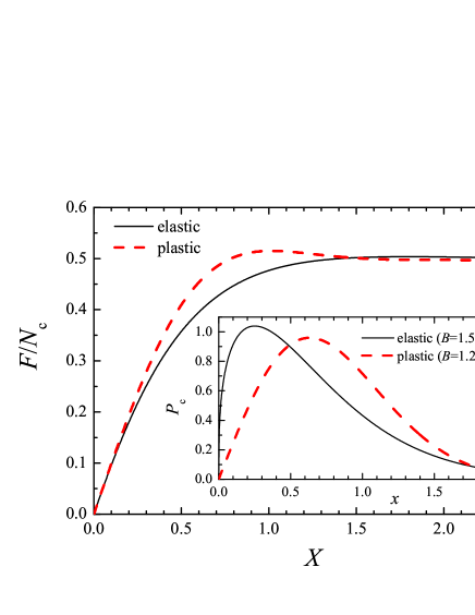
Figure 16: (Color online): Dependence of the friction force $F$ on $X$ for elastic ($B^{\prime}=1.588$, solid curve) and plastic ($B^{\prime\prime}=1.251$, broken curve) contacts with exponential distribution of heights. The initial distribution $Q_{\rm ini}(x)$ is Gaussian with $\bar{x}_{\rm ini}=0$ and $\sigma_{\rm ini}=0.025$. The inset shows the corresponding distributions $P_{c}(x)$, Eqs. (47) and (48).

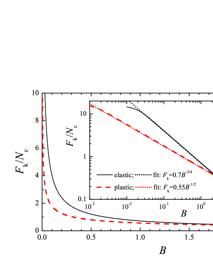
Figure 17: (Color online): Dependence of the kinetic friction $F_{k}$ in the smooth sliding state on the parameter $B$ for the elastic (solid curve) and plastic (broken curve) contacts. Inset: the same in log-log scale; dotted lines show power-law fits.

For a strong load, when the local stress exceeds the yield threshold $Y$, the contacts begin to deform plastically. When all contacts are plastic, the local pressure on contacts is $p_{\rm load}=H$, where $H$ is the hardness [$H\approx 3Y$ for the spherical geometry of asperities; for metals $H\approx(10^{-3}-10^{-2})E\sim 10^{9}$ Pa]. Then the normal force at the contact is $f_{l}(h)\approx\pi r(h-h_{0})H$. Assuming again that $f_{s}(h)\approx\mu f_{l}(h)$, we obtain

$$f_{s}=\pi r(h-h_{0})\mu H,$$ (46)

so that $\widetilde{P}_{c}(f_{s})\propto P_{h}\left[h(f_{s})\right]$ now.

For example, if we consider the exponential distribution of heights introduced by Greenwood and Williamson GW1966 to get analytical results $P_{h}(h)=\bar{h}^{-1}\exp(-h/\bar{h})\,\Theta(h)$, where $\bar{h}$ is the average height, then with Eq. (44) for the elastic contacts we obtain ($f,x>0$)

$$\widetilde{P}_{c}(f)\propto f^{-1/3}\exp(-B_{1}f^{2/3}),\;\;\;{\rm or}$$

$$P_{c}(x)\propto x^{{1}/{3}}\exp(-B^{\prime}x^{4/3}),$$ (47)

where $B_{1}=\left[(4\pi/3)^{2/3}\bar{h}r^{1/3}(\mu E^{*})^{2/3}\right]^{-1}$, while for the plastic contacts

$$\widetilde{P}_{c}(f)\propto\exp(-B_{2}f),\;\;\;{\rm or}\;\;\;P_{c}(x)\propto x\exp(-B^{\prime\prime}x^{2}),$$ (48)

where $B_{2}=(\pi\bar{h}r\mu H)^{-1}$. $B^{\prime}$ and $B^{\prime\prime}$ are numerical constants depending on the material.

The distributions $P_{c}(x)$ for elastic and plastic contacts, Eqs. (47) and (48), are presented in Fig. 16 (inset). We see that the force $F(X)$ increases (almost) monotonically with $X$, approaching the kinetic value $F_{k}$. Thus, in the case of a contact of rough surfaces, a relatively high concentration of low-threshold contacts prevents the stick-slip motion even for a very soft tribosystem (i.e., even in the case of a very low elastic constant of the driving spring $K$). The kinetic friction force $F_{k}$ depends on the parameter $B$ according to the power law (see Fig. 17), $F_{k}\propto B^{-3/4}\propto\bar{h}^{3/4}$ for the elastic contacts, and $F_{k}\propto B^{-1/2}\propto\bar{h}^{1/2}$ for the plastic contacts.

Similarly one can find $\widetilde{P}_{c}(f)$ for a more realistic Gaussian distribution of heights of the asperities GW1966 . In this case, the peak in the $P_{c}(x)$ dependence becomes narrower and higher, and the stick-slip regime may exist. Note that typical values for rough surfaces are of the order $r\sim 10-100$ $\mu$m, $\bar{h}\sim 1$ $\mu$m, so that the average size of the contact is $\bar{a}\approx\left(r\bar{h}\right)^{1/2}\sim 3-10$ $\mu$m BC2006 .

Whether the contacts are in the plastic or elastic regime, depends on the dimensionless parameter $\psi=(E/Y)(\bar{h}/r)^{1/2}$: $\psi\gg 1$, which is typical for metals, corresponds to the plastic regime while $\psi<1$ leads to an elastic regime, as, for instance, for rubber friction. Polymeric glasses belong to an intermediate situation, $\psi\gtrsim 1$, where only a fraction of contacts is plastic BC2006 .

VI.2 Rough surfaces: Persson’s model

The GW model used above completely ignores the elastic interaction between the contacts thus overestimating the role of low-threshold contacts. Recently Persson P2001a developed a contact mechanics theory which (indirectly) includes elastic interactions and leads to the correct low-threshold limit $\widetilde{P}_{c}(f\to 0)=0$. Although Persson’s theory is only rigorous for the case of complete contact (e.g., contact of rubber surfaces at high load), it leads to a very good agreement with experiments and simulations even for a contact of stiff surfaces and low loads YP2008 . Not going into details, note that the distribution of normal stresses $\sigma_{n}$ at the interface can approximately be described by an expression ($\sigma_{n}>0$)

$$P_{n}({\sigma_{n}})\propto\exp\left[-\left(\frac{\sigma_{n}-\bar{\sigma}_{n}}{\Delta\sigma_{n}}\right)^{2}\right]-\exp\left[-\left(\frac{\sigma_{n}+\bar{\sigma}_{n}}{\Delta\sigma_{n}}\right)^{2}\right],$$ (49)

where $\bar{\sigma}_{n}$ is the nominal squeezing pressure, the distribution width is given by $\Delta\sigma_{n}=E^{*}{\cal R}^{1/2}$, and the parameter ${\cal R}$ is determined by the roughness of the contacting surfaces,

$${\cal R}=\frac{1}{4\pi}\int dq\;q^{3}\int d^{2}x\;\langle h({\mathbf{x}})h({\mathbf{0}})\rangle e^{-i{\mathbf{q}}{\mathbf{x}}}.$$ (50)

Assuming that a local shear threshold is directly proportional to the local normal stress, $f_{s}\propto\sigma_{n}$, and again using Eq. (44), we finally obtain

$$P_{c}(x)\propto x\Bigg{\{} \exp\left[-\left(\frac{x^{2}-\bar{x}^{2}}{\sigma^{2}}\right)^{2}\right]$$ (51)

$$-\exp\left[-\left(\frac{x^{2}+\bar{x}^{2}}{\sigma^{2}}\right)^{2}\right]\Bigg{\}},$$

where $\sigma\propto(E^{*})^{1/2}{\cal R}^{1/4}$. The distribution (51) is characterized by a low concentration of small shear thresholds, $P_{c}(x)\propto x^{3}$ at $x\to 0$, and a fast decaying tail, $P_{c}(x)\propto\exp[-(x/\sigma)^{4}]$ at $x\to\infty$, i.e., the peaked structure of the distribution (51) is much more pronounced than in the GW model, Eqs. (47) and (48).

The numerical results are presented in Fig. 18 for two values of the roughness parameter. In contrast to the results of the GW model, they show a non-monotonous behavior of $F(X)$ which is compatible with a stick-slip motion.

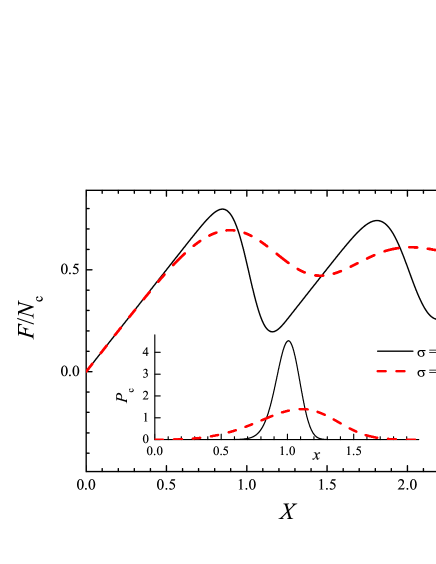
Figure 18: (Color online): Dependence of the friction force $F$ on $X$ for the Persson model with $\bar{x}=1$, $\sigma=0.5$ (solid) and $\sigma=1$ (broken curve). The initial distribution $Q_{\rm ini}(x)$ is Gaussian with $\bar{x}_{\rm ini}=0$ and $\sigma_{\rm ini}=0.025$. The inset shows the corresponding distributions $P_{c}(x)$, Eq. (51).

VI.3 Flat surfaces: dry friction

Let us now consider the dry contact of two flat surfaces. If both surfaces have an ideal crystalline structure, we get the singular case discussed in Appendix E. However such a situation is exceptional. A real surface always consists of domains, which are characterized by different crystalline orientation or even different structures.

MD simulations show a large variation of the static friction with the relative orientation of the two bare substrates HS1993 ; RS1996 , although surface irregularities as well as fluctuations of atomic positions at nonzero temperatures may mask this dependence QCCG2002 . A variation of the friction with the misfit angle was also observed experimentally, for instance in the FFM experiment made by Dienwiebel et al. DVPFHZ2004 .

In order to estimate a possible shape of the function $P_{c}(x)$ resulting from the domain structure of substrates, let us consider a rigid island (domain) of size $N_{a}$ with a triangular lattice placed onto a 2D periodic potential with square symmetry $V(x,y)=\sin x+\sin y$ created by the bottom substrate. The atomic coordinates of domain atoms are $\tilde{x}_{i}=X+(i+j/2)a$ and $\tilde{y}_{j}=Y+jh$, where $h=a\sqrt{3}/2$, $i=-j/2,\ldots,-j/2+n_{i}-1$, $j=0,\ldots,n_{j}-1$, $n_{i}n_{j}=N_{a}$ ($n_{i}a\approx n_{j}h$), and $X,Y$ are the center of mass coordinates. If the island is rotated by an angle $\phi$, then the atomic coordinates change to $x_{i}=\tilde{x}_{i}\cos\phi-\tilde{y}_{i}\sin\phi$ and $y_{i}=\tilde{x}_{i}\sin\phi+\tilde{y}_{i}\cos\phi$. For a fixed misfit angle $\phi$, the total potential energy of the domain is $U(X,Y)=\sum_{ij}V(x_{i},y_{j})$. Extrema (minima and saddle points) of the function $U(X,Y)$ are defined by $\partial U/\partial X=\partial U/\partial Y=0$; then the activation energy for domain motion is given by $\varepsilon_{a}=U_{\rm saddle}-U_{\rm min}$. Assuming that $f_{s}\sim\varepsilon_{a}/a_{s}\propto\varepsilon_{a}$, we can estimate the threshold force $f_{s}$ as a function of the misfit angle $\phi$ and the domain size $N_{a}$. This protocol was realized by Manini and Braun BM2010b . The calculation of a histogram of the function $\varepsilon_{a}(\phi)$ leads to the distribution $\widetilde{P}_{c}(f_{s})$, assuming that all domains have the same size $N_{a}$ and that all angles are equally present. Next, one may average over different domain sizes $N_{a}$, e.g., with a weight function $w(N_{a})=e^{-N_{a}/\bar{N}_{a}}$, where $\bar{N}_{a}$ is the average domain size. The distribution $\widetilde{P}_{c}(f)$ obtained in this way may be crudely approximated by the function $\widetilde{P}_{c}(f)\propto\exp(-f/\bar{f})$. Assuming that Eq. (44) holds, we come to the distribution

$$P_{c}(x)\propto x\exp(-x^{2}/\sigma^{2})\;,$$ (52)

which is similar to that of Fig. 16 characteristic for rough surfaces. Therefore in this system we again expect smooth sliding without stick-slip due to a large concentration of configurations with small barriers.

However, in the estimation we supposed that all angles are present with equal probability, while some angles could have preference due to their lower potential energy. Calculation shows that this would suppress the low-barrier thresholds so that the distribution $P_{c}(x)$ would become more peaked, and the stick-slip could exist.

VI.4 Lubricated surfaces: MD simulation

The dry-friction considered above is exceptional. In a real system, there is almost always a lubricant between the sliding surfaces (called “the third bodies” by tribologists) which is either a specially chosen lubricant film, grease (oil), dust, wear debris produced by sliding, or water or/and a thin layer of hydrocarbons adsorbed from air.

There is a large number of experimental and simulation studies of lubricated friction (e.g., see Refs. P0 ; BN2006 and references therein). A thin confined film (less than about six molecular diameters of thickness) typically solidifies thus producing nonzero static friction. The value of $f_{s}$ strongly depends on the film thickness and its structure, and moreover it may change with the time of stationary contact. In particular, Jabbarzadeh et al. JHT2006 have done the MD simulation of a thin lubrication film of dodecane. The transition from bulk liquid to high viscosity state when thickness decreases occurs at the thickness of six lubricant layers, and it appears due to formation of isolated crystalline bridges between the mica surfaces (across the film). As the thickness decreases further, these bridges increase in number and organize themselves into a mosaic structure with a long range orientational order. However in the previous MD study of the six-layer dodecane film between the mica substrates Jabbarzadeh et al. JHT2005 found also a “layer-over-layer” sliding regime with a very low friction. Such a configuration is found to be thermodynamically stable contrary to the metastable “bridge” configuration mentioned above. Thus, if the film is not ideally homogeneous along the interface but consists of domains of different structures and may be different thicknesses, it should be characterized by a distribution of static thresholds.

Moreover the top and bottom surfaces may be misoriented as well, as was mentioned above. In particular, He and Robbins studied the dependence of the static HR2001s and kinetic HR2001k friction on the rotation angle of the substrates for a lubricated system. It was observed that the static friction exhibits a peak at the commensurate angle ($\phi=0$) and then is approximately constant, the peak/plateau ratio being about 7 (for the monolayer lubricant film, for which the variation is the strongest).

A detailed study of the dependence of the static friction on the rotation angle $\phi$ for lubricant films of thickness from one to five layers has been done by Braun and Manini BM2010a . The value of $f_{s}$ varies with $\phi$ by more than one order in magnitude. When averaged over $\phi$ (assuming that all angles are present with the same probability) and also over film thickness with some weighting factor, the distribution of static thresholds may approximately be described by the function $\widetilde{P}_{c}(f)\propto f\exp(-f/\bar{f})$. Assuming again that Eq. (44) holds, we come to the distribution

$$P_{c}(x)\propto x^{3}\exp(-x^{2}/\sigma^{2})\;,$$ (53)

which would allow stick-slip.

VI.5 Lubricated surfaces: Lifshitz-Slözov coalescence

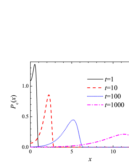
Figure 19: (Color online): Evolution of the distribution $P_{c}(x)$ with the time of stationary contact for the Lifshitz-Slözov coalescence mechanism ($\alpha=1$ and $B=1$).

In the conventional melting-freezing mechanism of friction, the lubricant is melted during slip, and solidifies when the motion stops. The solidification process can be described by the Lifshitz-Slözov theory (see LS1958 , Sec. 100). At the beginning, grains of solid phase emerge within the liquid lubricant film. Then the grains grow in size according to the law $\bar{r}\propto t^{1/3}$, where $\bar{r}$ is the average grain radius. The distribution of grains sizes is described by the following function: the number of grains with the radius from $r$ to $r+\Delta r$ is equal to $P_{\rm LS}(r/\bar{r})\,\Delta r/\bar{r}$, where the function $P_{\rm LS}(u)$ is zero for $u\geq 3/2$ (so that the maximum size of the grains is $1.5\bar{r}$), while lower sizes are distributed as

$$P_{\rm LS}(u)\propto\frac{u^{2}\exp\left[-1/(1-2u/3)\right]}{(u+3)^{7/3}\left(\frac{3}{2}-u\right)^{11/3}}\;.$$ (54)

Due to coalescence of grains, the total number of grains decreases with time as $N(t)\propto t^{-1}$. When the size of a grain exceeds the film thickness $d$ (that will occur when $\bar{r}(t)\geq d/3$ after the delay time $\tau_{m}\propto d^{3}$), such a grain will pin the surfaces. Using the relationship $\widetilde{P}_{c}(f)df\propto P_{\rm LS}(r/\bar{r})\,dr/\bar{r}$, we obtain that $\widetilde{P}_{c}(f)\propto(dr/df)P_{\rm LS}(r/\bar{r})/\bar{r}$. Because one grain gives the static threshold proportional to the contacting area, $f_{s}\propto\pi(r^{2}-d^{2}/4)$ for $r>d/2$, we have $dr/df\propto f^{-1/2}$. Combining all things together, we obtain that

$$P_{c}(x)=P_{\rm LS}(u),\;\;\;u=\rho^{-1}\left(1+Bx^{2}\right)^{1/2},$$ (55)

where $\rho(t)=2\bar{r}(t)/d=\alpha t^{1/3}$ (the pinning begins when $\rho>2/3$), and $B$ is determined by the system parameters (elasticity of the contacts, proportionality between the threshold $f_{s}$ and the area of the contacting grain, and the thickness of the lubricant film). The distribution (55) is shown in Fig. 19. Its shape suggests that it should lead to the conventional tribological behavior: the stick-slip motion at low driving velocity and smooth sliding at high velocities.

Thus, the described mechanism leads to a non-singular distribution of static thresholds and the typical stick-slip to smooth sliding behavior even for the case of ideal flat surfaces such as, e.g., the mica surfaces used in SFA experiments. Note that it incorporates both the delay time discussed in Appendix D and the aging of contacts considered in Sec. V; the latter, however, is a more complicated process than follows from the simplest Smoluchowsky theory.

In a general case, we also have to take into account that the lubricant film may consist of grains (domains) of different orientations or even different structures. Indeed, the proportionality coefficient in the relation $f_{s}\propto\pi(r^{2}-d^{2}/4)$ used above, should depend on the misfit angle between the lubricant domain and the substrate, so that the distribution $P_{\rm LS}(u)$ introduced above, additionally should depend on the misfit angle $\phi$, $P_{\rm LS}(u;\phi)$. Thus, if there are grains with different orientations, distributed according to a function $R_{\phi}(\phi)$, then

$$P_{c}(x)=\int d\phi\,R_{\phi}(\phi)P_{\rm LS}(u;\phi).$$ (56)

For example, if there are only two energetically equal possible orientations with $\phi=0$ and $\phi=\pi/4$, then $R_{\phi}(\phi)={1\over 2}\delta(\phi)+{1\over 2}\delta(\phi-\pi/4)$.

VII Conclusion

We introduced and analyzed in detail the earthquake-like model with a distribution of static thresholds. Reducing the problem to a master equation, we were able to find the exact solution numerically and even analytically in some important cases. Although, by its design, the ME approach should exactly correspond to the EQ model when the properties of the contacts are the same, it is difficult to give a formal proof of the equivalence of the two methods because the EQ model does not have a known analytical solution, except in very specific cases. The smooth sliding, as well as the transition from stick-slip to smooth sliding, emerge due to a finite width of the distribution $P_{c}(x)$ and have (almost) nothing in common with the melting-freezing or inertia microscopic mechanisms of stick-slip. We observed that, for stick slip to occur, the distribution of breaking thresholds $P_{c}(x)$ must have a low enough weight for small thresholds, for example, $P_{c}(x)\propto x^{3}$ if $x\to 0$ as follows from Eqs. (51) and (53).

The complex problem of behavior of a tribological system is split into two independent subproblems. In the present paper we studied the first one: dynamics of the friction contact, if the distribution of static thresholds $P_{c}(x)$ is known. The second separate problem is to find the distribution $\widetilde{P}_{c}(f)$ for a given system. Although we did not focus on this problem we examined the various possible situations of microscopic contacts to estimate $P_{c}(x)$ for those situations in order to examine how they fit in the framework of the master equation approach. For a contact of two hard rough surfaces (the multi-contact interface, or MCI in notations used by Baumberger and Caroli BC2006 ) this problem reduces to the statistics of asperities. The contact aging, i.e. the increase of static thresholds with the time of stationary contact, is due to two processes: the first (and more important) process is due to geometrical aging, or the increase of contact area at the asperity, and the second, due to structural aging, or restructuring of the contact. The value of the parameter $D$ in Eq. (41) may be estimated from experiments: it was found that in most cases the average static threshold $\mu_{s}=F_{s}/F_{\rm load}$ grows logarithmically with the waiting time $t_{w}$, $d\mu_{s}/d\,(\ln t_{w})\approx 10^{-2}$ BC2006 .

For flat surfaces such as, e.g., the mica surfaces used in the SFA experiments, the surface consists, most probably, of domains of different orientations (as for poly-crystals, and even for mono-crystals, where simply the sizes of domains are much larger). However, even if both sliding surfaces have an ideal crystalline structure on the macroscopic scale, anyway the lubricant film should consist of domains of different orientations or different metastable structures separated by dislocations (domain walls). The parameters of these domains can be studied by standard methods of molecular dynamics, while their evolution with time (the structural aging, which should lead to the increase of the static thresholds) may be described, e.g., by the Ginzburg-Landau theory.

It is interesting to note that the EQ-ME viewpoint discussed here appeared in biological physics more than fifty year ago to describe skeletal muscles  HS1971 . The Lacker-Peskin model P1975a ; P1975b ; LP1986 ; W1984 describes the binding-unbinding of the myosin molecules on actin filaments in terms of an equation which is very similar to our master equation.

Finally, let us mention questions which were not considered in the present work. First, throughout the paper we ignored inertia effects. They would imply that the distribution $Q(x)$ should be extended to negative $x$ values because some contacts could pick up enough kinetic energy during sliding to overshoot. Returning to the stick (pinned) state the spring force acting on such a contact would be negative P1995 . Moreover in the case of $dF_{k}(v)/dv<0$ which appears due to contacts aging, the regimes of stick-slip and smooth sliding may be separated by a regime of irregular (chaotic) motion due to inertia effects. Second, we completely ignored the role of the interaction between the contacts. The effects of interaction should change (increase) the critical velocity of the transition from stick-slip to smooth sliding. Interaction may be incorporated indirectly in a mean-field fashion by a renormalization of the distributions $P_{c}(x)$ and $R(x)$. However, a concerted, or synchronized breaking (triggering) of contacts may be studied numerically only within the earthquake-like model (e.g., see Ref. BR2002 ). It cannot be included rigorously in the master equation approach, unless it is coupled to a deformation field which deeply modifies the approach. Also, we considered the contacting planes of the sliding blocks as rigid planes, i.e., we ignored a possible variation (or fluctuation) of $F$ in the $(x,y)$ plane. Moreover, the latter should be coupled with the nonuniform elastic deformation of the block (for a preliminary work in this direction see Ref. BBU2009 ). Finally, we ignored a possible heating of the contacts due to sliding. All these question deserve separate studies. In conclusion, note that the approach developed in the present paper, is to be applied to meso- or macroscopic systems only and cannot be used to explain the AFM/FFM tip-based experiments, except if there is a multi-contact through a sufficient number of tip atoms.

Appendix A Shear elastic constant

To estimate possible values of the shear constant $k_{i}$, let us assume that the contacts have the shape of a cylinder of radius $r_{c}$ and length $h$ (i.e., $h$ is the thickness of the interface). Also, we suppose that one end of such a contact column is fixed, while a force $f_{i}$ is applied to the free end. This force will lead to the displacement $x_{i}=f_{i}/k_{i}$ of the end, where $k_{i}=3E_{c}I/h^{3}$, $E_{c}$ is the Young modulus of the material of the contact and $I=\pi r_{c}^{4}/4$ is the moment of inertia of the cylinder (see Ref. LL1986 ). This leads to

$$k_{i}=(3\pi/4)(E_{c}r_{c})(r_{c}/h)^{3}\,.$$ (57)

As the Young modulus is coupled with the transverse sound velocity of the material by the relationship $E_{c}=2\rho(1+\sigma)c^{2}$, where $\rho$ is the mass density and $\sigma$ is the Poisson ratio, we obtain

$$k_{i}=(3\pi/2)\rho(1+\sigma)c^{2}r_{c}(r_{c}/h)^{3}\,.$$ (58)

Thus, if $r_{c}\approx h$, we obtain $k_{i}\sim\rho c^{2}\sqrt{A_{i}}$, where $A_{i}=\pi r_{c}^{2}$ is the contact area.

Appendix B Two simple examples of steady state solutions

Figure 20: (Color online): The stationary distribution $Q_{s}(x)$ (blue dotted line), and the corresponding, numerically obtained, distribution of static thresholds $P_{xs}(x)$ (red broken line) for the rectangular distribution $P_{c}(x)$ (solid line).

As a simple example, let us consider the distribution $P(x)=p\;\Theta(x-x_{s})$, or

$$P(x)=\left\{\begin{array}[]{c}0\;\;\;{\rm if}\;\;\;x\leq x_{s},\\ p\;\;\;{\rm if}\;\;\;x>x_{s}.\end{array}\right.$$ (59)

One can easily find that $C=x_{s}+p^{-1}$,

$$E_{P}(x)=\left\{\begin{array}[]{ccc}1&{\rm for}&0\leq x\leq x_{s},\\ e^{-p(x-x_{s})}&{\rm for}&x>x_{s},\end{array}\right.$$ (60)

$$P_{c}(x)=\left\{\begin{array}[]{ccc}0&{\rm for}&0\leq x\leq x_{s},\\ p\,e^{-p(x-x_{s})}&{\rm for}&x>x_{s},\end{array}\right.$$ (61)

and

$$F_{k}={1\over 2}N_{c}\langle k_{i}\rangle\left[x_{s}+p^{-1}+p^{-1}/(1+px_{s})\right].$$ (62)

In particular, if $x_{s}=0$, then $Q_{s}(x)=\Theta(x)p\,e^{-px}$ and $F=N_{c}\langle k_{i}\rangle/p$, while for the case of $x_{s}>0$ and $p\to\infty$ we obtain that $Q_{s}(x)=x_{s}^{-1}$ within the interval $0\leq x\leq x_{s}$ and 0 outside it, so that $F={1\over 2}N_{c}\langle k_{i}\rangle x_{s}$.

Another simple example, which admits an exact solution, is the case of the rectangular $P_{c}(x)$ distribution shown in Fig. 20,

$$P_{c}(x)=\left\{\begin{array}[]{ll}0&{\rm if}\;\;\;x\leq 0.5,\\ 1&{\rm if}\;\;\;0.5<x<1.5,\\ 0&{\rm if}\;\;\;x\geq 1.5.\end{array}\right.$$ (63)

The fraction density of breaking contacts $P(x)$ is given by Eq. (6):

$$P(x)=\left\{\begin{array}[]{cl}0&{\rm if}\;\;\;x\leq 0.5,\\ (1.5-x)^{-1}&{\rm if}\;\;\;0.5<x<1.5,\\ \infty&{\rm if}\;\;\;x\geq 1.5.\end{array}\right.$$ (64)

$P(x)$, given by Eq. (6) diverges when $x$ tends to $1.5$, and then, according to its physical meaning it has to be infinite for larger values of $x$. In this case

$$U(x)=\left\{\begin{array}[]{cl}0&{\rm if}\;\;\;x\leq 0.5,\\ -\ln(1.5-x)&{\rm if}\;\;\;0.5<x<1.5,\\ \infty&{\rm if}\;\;\;x\geq 1.5,\end{array}\right.$$ (65)

$$E_{P}(x)=\left\{\begin{array}[]{cl}1&{\rm if}\;\;\;x\leq 0.5,\\ 1.5-x&{\rm if}\;\;\;0.5<x<1.5,\\ 0&{\rm if}\;\;\;x\geq 1.5.\end{array}\right.$$ (66)

The earthquake model with the distribution (63) and the master equation model with $P(x)$ given by Eq. (64) have exactly the same solution for any initial configuration.

Notice that this example clearly demonstrates that the probability distribution $P_{c}(x)$, which determines the static thresholds for the newborn contacts, is different from the distribution of static thresholds $P_{xs}(x)$ which is achieved in the steady state as pointed out in Sec. II.

Appendix C Friction loop

Figure 21: Friction loop. The distribution $P_{c}(x)$ is Gaussian with $\bar{x}_{s}=1$ and $\sigma_{s}=0.2$, the initial distribution $Q_{\rm ini}(x)$ is Gaussian with $\bar{x}_{\rm ini}=0$ and $\sigma_{\rm ini}=0.025$. The top substrate moves to the right, then to the left, and finally again to the right as indicated by arrows.

Through the paper we assumed that the top substrate moves continuously to the right, i.e. $\Delta X>0$. When the substrate moves to the left, or $\Delta X<0$, Eqs. (5), (7) and (8) must be modified in the following manner:

$$\Delta Q_{-}(x;X)=-P_{b}(x)\,\Delta\!X\,Q(x;X)\;,$$ (67)

$$\Delta Q_{+}(x;X)=R_{b}(x)\int_{-\infty}^{\infty}dx^{\prime}\,\Delta Q_{-}(x^{\prime};X)$$ (68)

and

$$\frac{\partial Q(x;X)}{\partial x}+\frac{\partial Q(x;X)}{\partial X}-P_{b}(x)\,Q(x;X)$$

$$=R_{b}(x)\int_{-\infty}^{\infty}dx^{\prime}\,P_{b}(x^{\prime})\,Q(x^{\prime};X),$$ (69)

where we have denoted by index $b$ ($P_{b}(x)$, $R_{b}(x)$) quantities relative to the backward motion. Comparing the equations for the forward and backward motions we see that they obey the symmetry relations $P_{b}(x)=P(-x)$ and $R_{b}(x)=R(-x)$ which are a manifestation of the irreversibility of the master equation. Indeed, if the force $f_{i}$ on a given contact $i$ approaches and overcomes $f_{si}$, the contact breaks; but if we now reverse the direction of the motion, this contact does not jump back to the value $f_{i}\approx f_{si}$; instead $f_{i}$ decreases until it reaches the value $f_{i}\approx-f_{si}$.

Although this comment does not bring in new physics, it is important for experimentalists. In a typical tribological experiment, the top substrate periodically moves forward and backward, and as a result, the so-called “friction loop” is observed. The same loop can easily be calculated with the ME approach as shown in Fig. 21.

Appendix D Delay effects

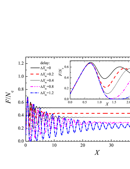
Figure 22: (Color online): The dependences $F(X)$ for different delay times $\Delta X_{m}=0$ (black solid), 0.2 (red dashed), 0.4 (black dotted), 0.8 (magenta dash-dot-dotted) and 1.2 (blue dash-dotted curve). The distribution $P_{c}(x)$ is Gaussian with $\bar{x}_{s}=1$ and $\sigma_{s}=0.2$, the initial distribution $Q_{\rm ini}(x)$ is Gaussian with $\bar{x}_{\rm ini}=0.1$ and $\sigma_{\rm ini}=0.025$, and $\langle k_{i}\rangle=1$.

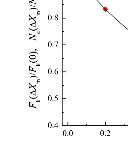
Figure 23: (Color online): The final number of asperities in contact (red circles) and the kinetic friction force (black diamonds) in smooth sliding regime as functions of the delay time (other parameters as in Fig. 22). The solid curve shows the $(1+\Delta X_{m})^{-1}$ dependence.

To establish Eq. (7) we assumed that, after a slip, a contact would stick again without any delay. Actually restoring the contact always requires a small delay $\tau_{m}$, particularly for the melting/freezing mechanism. Simulation BN2006 shows that $\tau_{m}\sim 10^{2}\tau_{0}$, where $\tau_{0}\sim 10^{-13}$s is a characteristic period of atomic oscillations in the lubricant. Therefore to write Eq. (7) we have to use $\Delta Q_{+}(x;X+\Delta\!X_{m})$, where $\Delta\!X_{m}=v\tau_{m}$ and $v$ is the driving velocity.

In the body of paper we ignored the delay effect. In this case $\Delta\!X_{m}=\Delta\!X$, and we may drop the $+\Delta\!X$ because it leads to a second order correction since it appears in a term which is already a correction to $Q$.

When the delay is taken into account, the integro-differential equation (8) has to be modified to become

$$\frac{\partial\widetilde{Q}(x;X)}{\partial x}+\frac{\partial\widetilde{Q}(x;X)}{\partial X}+P(x)\,\widetilde{Q}(x;X)$$

$$=R(x)\int_{-\infty}^{\infty}dx^{\prime}\,P(x^{\prime})\,\widetilde{Q}(x^{\prime};X-\Delta\!X_{m}).$$ (70)

The normalization condition (2) does not hold for $\widetilde{Q}(x;X)$ because the total number of unbroken contacts, is not conserved anymore. When an asperity breaks it is not in contact with the substrate during the time $\tau_{m}$ until the contact is restored. Thus, $N_{c}$ varies with $X$, and $N_{c}(X)<N_{c}(0)$, because some contacts are in a temporarily broken state even at smooth sliding. Typical dependences $F(X)$ for different values of the delay time are shown in Fig. 22. The kinetic friction force during smooth sliding is such that $F_{k}\propto N_{c}(\infty)$ and, therefore, it depends on pre–history of the contacts. If one starts from the same initial configuration, the final force $F_{k}$ is lower when the delay time increases (see Fig. 23). The dependence $F_{k}(v)$ is described by Eq. (42) with $F(\infty)=0$ and $v_{\rm aging}=\bar{x}_{s}/\tau_{m}$.

Appendix E The singular case

Figure 24: Evolution of the model for two $P_{c}(x)$ distributions: Left column is for a one-peak distribution of threshold, $P_{c}(x)=G(x;\bar{x},\sigma))$ with $\bar{x}=1$ and $\sigma=10^{-3}$ (i.e., close to the delta-function distribution), while right column is for a two-peak distribution of threshold, $P_{c}(x)={1\over 2}\left[G(x;0.95\bar{x},\sigma)+G(x;1.05\bar{x},\sigma)\right]$ (i.e., close to the distribution with two delta-functions). Solid curves show the distribution $Q(x;X)$ for incrementally increasing values of $X$ with the increment $\Delta X\approx 1$, dotted curves show $P_{c}(x)$ (for $X=0$ only). The bottom row shows the corresponding dependences $F(X)$ for $\langle k_{i}\rangle=1$ and $K=\infty$. The initial distribution $Q_{\rm ini}(x)$ is Gaussian with $\bar{x}_{\rm ini}=0.1$ and $\sigma_{\rm ini}=0.025$.

As we have shown, in a general case the solution of the master equation always approaches the steady-state solution given by Eqs. (12–14), which describes the smooth sliding. However, there is one exception from this general scenario, when the model admits a periodic solution and $F(X)\neq$ Const even in the limit $X\to\infty$. This is the singular case when all contacts are identical, i.e., all contacts are characterized by the same static threshold $x_{s}$, so that $P_{c}(x)=\delta(x-x_{s})$, or $P(x)=0$ for $x<x_{s}$ and $P(x)=\infty$ for $x\geq x_{s}$.

As one can check by direct substitution, in this particular case the steady-state solution of Eq. (8) has the following form:

$$Q(x;X)=S(x-X)\left[\Theta(x)-\Theta(x-x_{s})\right],$$ (71)

where the function $S(\xi)$ is defined by the initial condition: $S(\xi)=Q_{\rm ini}(\xi)$ for the interval $0\leq\xi<x_{s}$, and then $S(\xi)$ should be repeated periodically over the whole interval $-\infty\leq\xi<\infty$,

$$S(\xi\pm nx_{s})=S(\xi)\quad\forall\;n~{}{\mathrm{integer}}\;.$$

In this simple case the total force (3) is equal to

$$F(X)=N_{c}k\left[X+\int_{-X}^{x_{s}-X}d\xi\,\xi S(\xi)\right].$$ (72)

The static friction force takes the minimal value $F_{s}={1\over 2}N_{c}kx_{s}$ for the uniform initial distribution, $Q_{\rm ini}(x)=x_{s}^{-1}$, when $F(X)$ does not depend on $X$, and the maximal value $F_{s}=N_{c}kx_{s}$ for the delta-function initial distribution $Q_{\rm ini}(x)=\delta(x-x_{0})$ with some $0\leq x_{0}<x_{s}$, when the function $F(X)$ has sawtooth shape changing from 0 to $F_{s}$.

However, the periodic solution described above only exists for a distribution $P_{c}(x)$ with a single threshold. If the contacts are characterized by more than one threshold value, for example, if one part of contacts has the threshold $x_{s1}$ and another part the threshold $x_{s2}\neq x_{s1}$ [i.e., $P_{c}(x)$ is described by a sum of two delta-functions], then the system will always approach the stationary steady state. This is demonstrated in Fig. 24, where we compare the system evolution in cases of one-peak and two-peak $P_{c}(x)$ distributions. Notice, however, that this statement is only valid for an infinite set of contacts (the number of contacts with each threshold must be infinite) and cannot be applied for a microscopic system where, e.g. two tips move over a surface.

References

- (1) B.N.J. Persson, Sliding Friction: Physical Principles and Applications (Springer-Verlag, Berlin, 1998).
- (2) M.H. Müser, M. Urbakh, and M.O. Robbins, Adv. Chem. Phys. 126, 187 (2003).
- (3) O.M. Braun and A.G. Naumovets, Surf. Sci. Reports 60, 79 (2006).
- (4) T. Baumberger and C. Caroli, Advances in Physics 55, 279 (2006).
- (5) M.O. Robbins and P.A. Thompson, Science 253, 916 (1991).
- (6) O.M. Braun and M. Peyrard, Phys. Rev. E63, 046110 (2001).
- (7) O.M. Braun and J. Röder, Phys. Rev. Lett. 88, 096102 (2002).
- (8) O.M. Braun, M. Peyrard, V. Bortolani, A. Franchini, and A. Vanossi, Phys. Rev. E72, 056116 (2005).
- (9) F. Heslot, T. Baumberger, B. Perrin, B. Caroli, and C. Caroli, Phys. Rev. E49, 4973 (1994); T. Baumberger, C. Caroli, B. Perrin, and O. Ronsin, Phys. Rev. E51, 4005 (1995).
- (10) B.N.J. Persson, Phys. Rev. B55, 8004 (1997).
- (11) R. Burridge and L. Knopoff, Bull. Seismol. Soc. Am. 57, 341 (1967).
- (12) J.M. Carlson and J.M. Langer, Phys. Rev. Lett. 62, 2632 (1989).
- (13) Z. Olami, H.J.S. Feder, and K. Christensen, Phys. Rev. Lett. 68, 1244 (1992).
- (14) B.N.J. Persson, Phys. Rev. B51, 13568 (1995).
- (15) A.E. Filippov, J. Klafter, and M. Urbakh, Phys. Rev. Lett. 92, 135503 (2004).
- (16) Z. Farkas, S.R. Dahmen, and D.E. Wolf, J. Stat. Mech.: Theory and Experiment P06015 (2005); cond-mat/0502644.
- (17) O.M. Braun and M. Peyrard, Phys. Rev. Lett. 100, 125501 (2008).
- (18) O.M. Braun and E. Tosatti, Europhys. Lett. 88, 48003 (2009).
- (19) O.M. Braun, I. Barel, and M. Urbakh, Phys. Rev. Lett. 103, 194301 (2009).
- (20) H. Yoshizawa, Y. L. Chen, and J. Israelachvili, Wear 168, 161 (1993); H. Yoshizawa and J. Israelachvili, J. Phys. Chem. 97, 11300 (1993).
- (21) J.A. Greenwood and J.B.P. Williamson, Proc. Roy. Soc. A 295, 300 (1966).
- (22) A. Garg, Phys. Rev. B51, 15592 (1995).
- (23) O.K. Dudko, A.E. Filipov, J. Klafter, and M. Urbakh, PNAS 100, 11378 (2003).
- (24) M. Srinivasan and S. Walcott, Phys. Rev. E80, 046124 (2009).
- (25) H. Yoshizawa, P. McGuiggan, and J. Israelachvili, Science 259, 1305 (1993).
- (26) S. Sills and R.M. Overney, Phys. Rev. Lett. 91, 095501 (2003).
- (27) A. Schirmeisen, L. Jansen, H. Hölscher, and H. Fuchs, Apl. Phys. Lett. 88, 123108 (2006).
- (28) A. Maeda, Y. Inoue, H. Kitano, S. Okayasu, and I. Tsukada, Int. J. Mod. Phys. B 19, 463 (2005).
- (29) A. Maeda, Y. Inoue, H. Kitano, S. Savel’ev, S. Okayasu, I. Tsukada, and F. Nori, Phys. Rev. Lett. 94, 077001 (2005).
- (30) A. Maeda and D. Nakamura, Journal of Physics: Conference Series 89, 012020 (2007).
- (31) D. Nakamura, T. Kubo, S. Kitamura, L.B. Gómez, A. Maeda, M. Konczykowski, and C.J. van der Beek, Journal of Physics: Conference Series 89, 012021 (2007).
- (32) K.L. Johnson, Contact Mechanics (Cambridge University Press, Cambridge, 1985).
- (33) B.N.J. Persson, J. Chem. Phys. 115, 3840 (2001).
- (34) C. Yang and B.N.J. Persson, J. Phys.: Condens. Matter 20, 215214 (2008).
- (35) M. Hirano and K. Shinjo, Wear 168, 121 (1993).
- (36) M.O. Robbins and E.D. Smith, Langmuir 12, 4543 (1996).
- (37) Y. Qi, Y.-T. Cheng, T. Cagin, and W.A. Goddard III, Phys. Rev. B66, 085420 (2002).
- (38) M. Dienwiebel, G.S. Verhoeven, N. Pradeep, J.W.M. Frenken, J.A. Heimberg, and H.W. Zandbergen, Phys. Rev. Lett. 92, 126101 (2004).
- (39) N. Manini and O.M. Braun, Phys. Rev. E, submitted (manuscript ET10772) (2010).
- (40) A. Jabbarzadeh, P. Harrowell, and R.I. Tanner, Phys. Rev. Lett. 96, 206102 (2006).
- (41) A. Jabbarzadeh, P. Harrowell, and R.I. Tanner, Phys. Rev. Lett. 94, 126103 (2005).
- (42) G. He and M.O. Robbins, Phys. Rev. B64, 35413 (2001).
- (43) G. He and M.O. Robbins, Tribology Letters 10, 7 (2001).
- (44) O.M. Braun and N. Manini, Phys. Rev. E, submitted (manuscript EM10550) (2010).
- (45) E.M. Lifshitz and L.P. Pitaevskii, Physical Kinetics (Pergamon, Oxford, 1981).
- (46) A.F. Huxley and R.M. Simmons, Nature (London) 233, 533 (1971).
- (47) C.S. Peskin, Lectures on Mathematical Aspects of Physiology (Courant Institute of Mathematical Sciences, New York, 1975).
- (48) C.S. Peskin, Mathematical Aspects of Heart Physiology (Courant Institute of Mathematical Sciences, New York, 1975).
- (49) H.M. Lacker and C.S. Peskin, Lect. Math Life Sci. (American Mathematical Society, Providence, RI, 1986), Vol. 16, p. 121.
- (50) W.O. Williams, Mathematical Biosciences 70, 203 (1984).
- (51) L.D. Landau and E.M. Lifshitz, Theory of Elasticity, Course of Theoretical Physics Vol. 7 (Pergamon, New York, 1986).