Mixing of fermion fields of opposite parities and baryon resonances

Abstract

We consider a loop mixing of two fermion fields of opposite parities whereas the parity is conserved in a Lagrangian. Such kind of mixing is specific for fermions and has no analogy in boson case. Possible applications of this effect may be related with physics of baryon resonances. The obtained matrix propagator defines a pair of unitary partial amplitudes which describe the production of resonances of spin $J$ and different parity ${1/2}^{\pm}$ or ${3/2}^{\pm}$.
The use of our amplitudes for joint description of $\pi N$ partial waves $P_{13}$ and $D_{13}$ shows that the discussed effect is clearly seen in these partial waves as the specific form of interference between resonance and background. Another interesting application of this effect may be a pair of partial waves $S_{11}$ and $P_{11}$ where the picture is more complicated due to presence of several resonance states.

I Introduction

Mixing of states (fields) is a well-known phenome- non existing in the systems of neutrinos Pon58 , quarks Cab63 and hadrons. In hadron systems the mixing effects are essential not only for $K^{0}$- and $D^{0}$-mesons but also for the broad overlapping resonances. As for theoretical description of mixing phenomena, a general tendency with time and development of experiment consists in transition from a simplified quantum-mechanical description to the quantum field theory methods (see e.g. review Beu03 , more recent papers Esp02 ; Bla04 ; Mac05 ; Kni06 ; Dur08 and references therein).

Mixing of fermion fields has some specifics as compared with boson case. Firstly, there exists $\gamma$-matrix structure in a propagator. Secondly, fermion and antifermion have the opposite $P$-parity, so fermion propagator contains contributions of different parities. As a result, besides a standard mixing of fields with the same quantum numbers, for fermions there exists a mixing of fields with opposite parities (OPF-mixing), even if the parity is conserved in Lagrangian.

Such a possibility for fermion mixing has been noted in Kal06 . In this paper we study this effect in detail and apply it to the baryon resonances production in $\pi N$ reaction.

In section 2 we consider a standard mixing of fermion fields of the same parity. Following to Kal04 ; Kal06 ; Gon07 we use the off-shell projection basis to solve the Dyson–Schwinger equation, it simplilies all manipulations with $\gamma$-matrices and, moreover, clarifies the meaning of formulas. The use of this basis leads to separation of $\gamma$-matrix structure, so in standard case we come to studying of a mixing matrix, which is very similar to boson mixing matrix.

In section 3 we derive a general form of matrix dressed propagator with accounting of the OPF-mixing. In contrast to standard case the obtained propagator contains $\gamma^{5}$ terms, even if parity is conserved in vertexes.

Section 4 is devoted to more detailed studying of considered OPF-mixing in application to production of resonances $J^{P}={1/2}^{\pm},I=1/2$ in $\pi N$ scattering. First estimates demonstrates that the considered mixing generates marked effects in $\pi N$ partial waves, changing a typical resonance curve. Comparison of the obtained multichannel hadron amplitudes with $K$-matrix parameterization shows that our amplitudes may be considered as a specific variant of analytical $K$-matrix.

In section 5 we consider OPF-mixing for case of two vector-spinor Rarita-Schwinger fields $\Psi^{\mu}$, describing spin-$3/2$ particles, and apply the obtained hadron amplitudes for descriptions of $\pi N$ partial waves $P_{13}$ and $D_{13}$.

Conclusion contains discussion of results.

In Application there are collected some details of calculations, concerning the production of spin-$3/2$ resonances.

II Mixing of fermion fields of the same parity

Let us start from the standard picture when the mixing fermions have the same quantum numbers. To obtain the dressed fermion propagator $G(p)$ one should perform the Dyson summation or, equivalently, to solve the Dyson–Schwinger equation:

$$G(p)=G_{0}+G\Sigma G_{0},$$ (1)

where $G_{0}$ is a free propagator and $\Sigma$ is a self-energy:

$$\Sigma(p)=A({p}^{2})+\widehat{p}B({p}^{2}).$$ (2)

We will use the off-shell projection operators $\Lambda^{\pm}$:

$$\Lambda^{\pm}=\frac{1}{2}\Big{(}1\pm\frac{\hat{p}}{W}\Big{)},$$

where $W=\sqrt{p^{2}}$ is energy in the rest frame.

Main properties of projection operators are:

$$\Lambda^{\pm}\Lambda^{\pm}=\Lambda^{\pm},\quad\Lambda^{\pm}\Lambda^{\mp}=0,\quad\Lambda^{\pm}\gamma^{5}=\gamma^{5}\Lambda^{\mp},$$

$$\Lambda^{+}+\Lambda^{-}=1,\quad\Lambda^{+}-\Lambda^{-}=\frac{\hat{p}}{W}.$$

Let us rewrite the equation (1) expanding all elements in the basis of projection operators:

$$G=\sum_{M=1}^{2}\mathcal{P}_{M}G^{M},$$ (3)

where we have introduced the notations:

$$\mathcal{P}_{1}=\Lambda^{+},\quad\mathcal{P}_{2}=\Lambda^{-}.\quad$$

In this basis the Dyson–Schwinger equation is reduced to equations on scalar functions:

$$G^{M}=G^{M}_{0}+G^{M}\Sigma^{M}G^{M}_{0},\qquad M=1,2,$$ (4)

or

$$\Big{(}G^{-1}\Big{)}{\vphantom{G^{-1}}}^{M}=\Big{(}G^{-1}_{0}\Big{)}{\vphantom{G^{-1}}}^{M}-\Sigma^{M}.\$$ (5)

The solution of (4) for dressed propagator looks like:

$$\begin{split}\Big{(}G^{-1}\Big{)}{\vphantom{G^{-1}}}^{1}&=\Big{(}G^{-1}_{0}\Big{)}{\vphantom{G^{-1}}}^{1}-\Sigma^{1}=W-m-A(W^{2})-WB(W^{2}),\\ \Big{(}G^{-1}\Big{)}{\vphantom{G^{-1}}}^{2}&=\Big{(}G^{-1}_{0}\Big{)}{\vphantom{G^{-1}}}^{2}-\Sigma^{2}=-W-m-A(W^{2})+WB(W^{2})\end{split}$$ (6)

where $A$, $B$ are commonly used components of the self-energy. The coefficients in the projection basis have the obvious property:

$$\Sigma^{2}(W)=\Sigma^{1}(-W).$$

When we have two fermion fields $\Psi_{i}$ , the including of interaction leads also to mixing of these fields. In this case the Dyson–Schwinger equation (1) acquire matrix indices:

$$G_{ij}=(G_{0})_{ij}+G_{ik}\Sigma_{kl}(G_{0})_{lj},\quad i,j,k,l=1,2.$$ (7)

Therefore one can use the same equation (1) assuming all coefficients to be matrices.

The simplest variant is when the fermion fields $\Psi_{i}$ have the same quantum numbers and the parity is conserved in the Lagrangian. In this case the inverse propagator following (5) has the form:

$$\begin{split}G^{-1}&=\mathcal{P}_{1}S^{1}(W)+\mathcal{P}_{2}S^{2}(W)=\\[8.53581pt] &=\mathcal{P}_{1}\begin{pmatrix}W-m_{1}-\Sigma^{1}_{11}&-\Sigma^{1}_{12}\\ -\Sigma^{1}_{21}&W-m_{2}-\Sigma^{1}_{22}\end{pmatrix}+\\[8.53581pt] &+\mathcal{P}_{2}\begin{pmatrix}-W-m_{1}-\Sigma^{2}_{11}&-\Sigma^{2}_{12}\\ -\Sigma^{2}_{21}&-W-m_{2}-\Sigma^{2}_{22}\end{pmatrix}.\end{split}$$ (8)

The matrix coefficients as before have the symmetry property $S^{2}(W)=S^{1}(-W)$. To obtain the matrix dressed propagator $G(p)$ one should reverse the matrix coefficients in projection basis:

$$\begin{split}G(p)&=\mathcal{P}_{1}(S^{1}(W))^{-1}+\mathcal{P}_{2}(S^{2}(W))^{-1}=\\[8.53581pt] &=\mathcal{P}_{1}\begin{pmatrix}\dfrac{W-m_{2}-\Sigma^{1}_{22}}{\Delta_{1}}&-\dfrac{\Sigma^{1}_{12}}{\Delta_{1}}\\[11.38109pt] -\dfrac{\Sigma^{1}_{21}}{\Delta_{1}}&\dfrac{W-m_{1}-\Sigma^{1}_{11}}{\Delta_{1}}\end{pmatrix}+\\[8.53581pt] &+\mathcal{P}_{2}\begin{pmatrix}\dfrac{-W-m_{2}-\Sigma^{2}_{22}}{\Delta_{2}}&-\dfrac{\Sigma^{2}_{12}}{\Delta_{2}}\\[11.38109pt] -\dfrac{\Sigma^{2}_{21}}{\Delta_{2}}&\dfrac{-W-m_{1}-\Sigma^{2}_{11}}{\Delta_{2}}\end{pmatrix},\end{split}$$ (9)

where

$$\begin{split}\Delta_{1}&=\big{(}W-m_{1}-\Sigma^{1}_{11}\big{)}\big{(}W-m_{2}-\Sigma^{2}_{22}\big{)}-\Sigma^{4}_{12}\Sigma^{3}_{21},\\ \Delta_{2}&=\big{(}-W-m_{1}-\Sigma^{2}_{11}\big{)}\big{(}-W-m_{2}-\Sigma^{1}_{22}\big{)}-\Sigma^{3}_{12}\Sigma^{4}_{21}=\Delta_{1}\big{(}W\to-W\big{)}.\end{split}$$

We see that with use of projection basis the problem of fermion mixing is reduced to studying of the same mixing matrix as for bosons besides the obvious replacement $s-m^{2}\rightarrow W-m$.

III Mixing of fermion fields of opposite P-parities

Let us consider the joint dressing of two fermion fields of opposite parities provided that the parity is conserved in a vertex. In this case the diagonal transition loops $\Sigma_{ii}$ contain only $I$ and $\hat{p}$ matrices, while the off-diagonal ones $\Sigma_{12},\Sigma_{21}$ must contain $\gamma^{5}$. Projection basis should be supplemented by elements containing $\gamma^{5}$, it is convenient to choose the $\gamma$-matrix basis as:

$$\mathcal{P}_{1}=\Lambda^{+},\quad\mathcal{P}_{2}=\Lambda^{-},\quad\mathcal{P}_{3}=\Lambda^{+}\gamma^{5},\quad\mathcal{P}_{4}=\Lambda^{-}\gamma^{5}.\quad$$ (10)

In this case the $\gamma$-matrix decomposition has four terms:

$$S=\sum_{M=1}^{4}\mathcal{P}_{M}S^{M},$$ (11)

where the coefficients $S^{M}$ are matrices and have the obvious symmetry properties:

$$S^{2}(W)=S^{1}(-W),\quad S^{4}(W)=S^{3}(-W).$$ (12)

Inverse propagator in this basis looks as:

$$\begin{split}S(p)&=\mathcal{P}_{1}\begin{pmatrix}W-m_{1}-\Sigma^{1}_{11}&0\\ 0&W-m_{2}-\Sigma^{1}_{22}\end{pmatrix}+\\[8.53581pt] &+\mathcal{P}_{2}\begin{pmatrix}-W-m_{1}-\Sigma^{2}_{11}&0\\ 0&-W-m_{2}-\Sigma^{2}_{22}\end{pmatrix}+\\[8.53581pt] &+\mathcal{P}_{3}\begin{pmatrix}0&-\Sigma^{3}_{12}\\ -\Sigma^{3}_{21}&0\end{pmatrix}+\mathcal{P}_{4}\begin{pmatrix}0&-\Sigma^{4}_{12}\\ -\Sigma^{4}_{21}&0\end{pmatrix},\end{split}$$ (13)

where the indexes $i,j=1,2$ in the self-energy $\Sigma^{M}_{ij}$ numerate dressing fermion fields and the indexes $M={1,\dots 4}$ are refered to the $\gamma$-matrix decomposition (11).

Elements of the basis (10) have simple multiplicative properties (see Table 1), so reversing of (13) present no special problems Kal06 .

Table 1: Multiplicative properties of elements of basis (10).

	$\mathcal{P}_{1}$	$\mathcal{P}_{2}$	$\mathcal{P}_{3}$	$\mathcal{P}_{4}$
$\mathcal{P}_{1}$	$\mathcal{P}_{1}$	0	$\mathcal{P}_{3}$	0
$\mathcal{P}_{2}$	0	$\mathcal{P}_{2}$	0	$\mathcal{P}_{4}$
$\mathcal{P}_{3}$	0	$\mathcal{P}_{3}$	0	$\mathcal{P}_{1}$
$\mathcal{P}_{4}$	$\mathcal{P}_{4}$	0	$\mathcal{P}_{2}$	0

Reversing of (13) gives the matrix dressed propagator of the form:

$$\begin{split}G=&\mathcal{P}_{1}\begin{pmatrix}\dfrac{-W-m_{2}-\Sigma^{2}_{22}}{\Delta_{1}}&0\\ 0&\dfrac{-W-m_{1}-\Sigma^{2}_{11}}{\Delta_{2}}\end{pmatrix}+\\[8.53581pt] +&\mathcal{P}_{2}\begin{pmatrix}\dfrac{W-m_{2}-\Sigma^{1}_{22}}{\Delta_{2}}&0\\ 0&\dfrac{W-m_{1}-\Sigma^{1}_{11}}{\Delta_{1}}\end{pmatrix}+\\[8.53581pt] +&\mathcal{P}_{3}\begin{pmatrix}0&\dfrac{\Sigma^{3}_{12}}{\Delta_{1}}\\ \dfrac{\Sigma^{3}_{21}}{\Delta_{2}}&0\end{pmatrix}+\mathcal{P}_{4}\begin{pmatrix}0&\dfrac{\Sigma^{4}_{12}}{\Delta_{2}}\\ \dfrac{\Sigma^{4}_{21}}{\Delta_{1}}&0\end{pmatrix}.\end{split}$$ (14)

Here

$$\begin{split}\Delta_{1}&=\big{(}W-m_{1}-\Sigma^{1}_{11}\big{)}\big{(}-W-m_{2}-\Sigma^{2}_{22}\big{)}-\Sigma^{3}_{12}\Sigma^{4}_{21},\\ \Delta_{2}&=\big{(}-W-m_{1}-\Sigma^{2}_{11}\big{)}\big{(}W-m_{2}-\Sigma^{1}_{22}\big{)}-\Sigma^{4}_{12}\Sigma^{3}_{21}=\Delta_{1}\big{(}W\to-W\big{)}.\end{split}$$

The propagator (14) can be compared with the standard case of mixing (fermion fields of the same parity) (9).

IV $\pi N$ scattering and mixing of baryons $1/2^{\pm}$

As for possible applications of considered effect to description of baryon resonances, this is, first of all, $\pi N$ scattering, where the high accuracy data exist and detailed partial wave analysis has been performed Cut79 ; Koc85 ; Hoh93 ; Arn95 ; Arn06 .

IV.1 Partial waves

Let us consider an effect of OPF-mixing on the production of baryon resonances of spin-parity $J^{P}={1/2}^{\pm}$ and isospin $I=1/2$ in $\pi N$-collisions.

Simplest effective Lagrangians have the form:

$$\mathscr{L}_{int} =\mathrm{i}\,g_{1}\bar{N}_{1}(x)\gamma^{5}N(x)\phi(x)+\text{h.c.} \text{for }J^{P}(N_{1})={1/2}^{+},$$

$$\mathscr{L}_{int} =g_{2}\bar{N}_{2}(x)N(x)\phi(x)+\text{h.c.} \text{for }J^{P}(N_{2})={1/2}^{-}.$$

In $n$-channel case, the scattering amplitude is a matrix of dimension $n$:

$$T=\bar{u}(p_{2},s_{2})Ru(p_{1},s_{1}),$$ (15)

where $\bar{u}(p_{2},s_{2})$ and $u(p_{1},s_{1})$ are four-component spinors, corresponding to final and initial nucleon, and $R$ is matrix of the same dimension $n$ consisting of the propagator and coupling constants.

In the two-channel approximation ($\pi N$ and $\eta N$ channel) matrix $R$ is of the form:

$$R=-\begin{pmatrix}\mathrm{i}\,g_{1,\pi}\gamma^{5}&g_{2,\pi}\\ \mathrm{i}\,g_{1,\eta}\gamma^{5}&g_{2,\pi}\end{pmatrix}\times G\times\begin{pmatrix}\mathrm{i}\,g_{1,\pi}\gamma^{5}&\mathrm{i}\,g_{1,\eta}\gamma^{5}\\ g_{2,\pi}&g_{2,\eta}\end{pmatrix},$$ (16)

and generalization for $n$ channels and $m$ mixed states is obvious. Here $G$ is dressed propagator (14) and we have introduced the short notations for coupling constants: $g_{1,\pi}\equiv g_{N_{1}\pi N}$, $g_{2,\pi}\equiv g_{N_{2}\pi N}$.

After some algebra the matrix $R$ turns into into the standard form

$$R=\Lambda^{+}R_{1}+\Lambda^{-}R_{2},$$ (17)

where $R_{1}$ and $R_{2}$ are dimension 2 matrices. Note that the $\gamma^{5}$ matrix has been disappeared after multiplication in (16), since parity is not violated. After it we obtain from (15) the two-channel $s$- and $p$- partial waves.

$s$-waves amplitudes (produced resonances have $J^{P}={1/2}^{-}$) in standard notations have the form:

$$\begin{split}f_{s,+}(\pi N\rightarrow\pi N)&=\frac{(E_{1}+m_{N})}{8\pi W\Delta_{2}}\Big{[}g^{2}_{1,\pi}(W-m_{2}-\Sigma^{1}_{22})-g^{2}_{2,\pi}(-W-m_{1}-\Sigma^{2}_{11})-\\ &-\mathrm{i}\,g_{1,\pi}g_{2,\pi}(\Sigma^{3}_{21}+\Sigma^{4}_{12})\Big{]},\\ f_{s,+}(\pi N\rightarrow\eta N)&=\frac{\sqrt{(E_{1}+m_{N})(E_{2}+m_{N})}}{8\pi W\Delta_{2}}\Big{[}g_{1,\pi}g_{1,\eta}(W-m_{2}-\Sigma^{1}_{22})-\\ &-g_{2,\pi}g_{2,\eta}(-W-m_{1}-\Sigma^{2}_{11})-\mathrm{i}\,g_{2,\eta}g_{1,\pi}\Sigma^{3}_{21}-\mathrm{i}\,g_{1,\eta}g_{2,\pi}\Sigma^{4}_{12}\Big{]},\\ f_{s,+}(\eta N\rightarrow\eta N)&=\frac{(E_{2}+m_{N})}{8\pi W\Delta_{2}}\Big{[}g^{2}_{1,\eta}(W-m_{2}-\Sigma^{1}_{22})-g^{2}_{2,\eta}(-W-m_{1}-\Sigma^{2}_{11})-\\ &-\mathrm{i}\,g_{1,\eta}g_{2,\eta}(\Sigma^{3}_{21}+\Sigma^{4}_{12})\Big{]},\\ \Delta_{2}&=\big{(}-W-m_{1}-\Sigma^{2}_{11}\big{)}\big{(}W-m_{2}-\Sigma^{1}_{22}\big{)}-\Sigma^{4}_{12}\Sigma^{3}_{21},\end{split}$$ (18)

where $E_{1}$ and $E_{2}$ are nucleon energy in the c.m.s. for $\pi N$ and $\eta N$ respectively.

For comparison, we write down the amplitude $\pi N\rightarrow\pi N$ in a tree approximation:

$$f_{s,+}^{\text{tree}}(\pi N\rightarrow\pi N)=\dfrac{(E_{1}+m_{N})}{8\pi W}\Big{[}\dfrac{g^{2}_{1,\pi}}{(-W-m_{1})}-\dfrac{g^{2}_{2,\pi}}{(W-m_{2})}\Big{]}.$$ (19)

Simultaneous calculation of $p$-wave amplitudes ($J^{P}={1/2}^{+}$) gives:

$$\begin{split}f_{p,-}(\pi N\rightarrow\pi N)&=-\frac{(E_{1}-m_{N})}{8\pi W\Delta_{1}}\Big{[}g^{2}_{1,\pi}(-W-m_{2}-\Sigma^{2}_{22})-g^{2}_{2,\pi}(W-m_{1}-\Sigma^{1}_{11})-\\ &-\mathrm{i}\,g_{1,\pi}g_{2,\pi}(\Sigma^{4}_{21}+\Sigma^{3}_{12})\Big{]},\\ f_{p,-}(\pi N\rightarrow\eta N)&=-\frac{\sqrt{(E_{1}-m_{N})(E_{2}-m_{N})}}{8\pi W\Delta_{1}}\Big{[}g_{1,\pi}g_{1,\eta}(-W-m_{2}-\Sigma^{2}_{22})-\\ &-g_{2,\pi}g_{2,\eta}(W-m_{1}-\Sigma^{1}_{11})-\mathrm{i}\,g_{2,\eta}g_{1,\pi}\Sigma^{4}_{21}-\mathrm{i}\,g_{1,\eta}g_{2,\pi}\Sigma^{3}_{12}\Big{]},\\ f_{p,-}(\eta N\rightarrow\eta N)&=-\frac{(E_{2}-m_{N})}{8\pi W\Delta_{1}}\Big{[}g^{2}_{1,\eta}(-W-m_{2}W-\Sigma^{2}_{22})-g^{2}_{2,\eta}(W-m_{1}-\Sigma^{1}_{11})-\\ &-\mathrm{i}\,g_{1,\eta}g_{2,\eta}(\Sigma^{4}_{21}+\Sigma^{3}_{12})\Big{]},\\ \Delta_{1}&=\big{(}W-m_{1}-\Sigma^{1}_{11}\big{)}\big{(}-W+m_{2}-\Sigma^{2}_{22}\big{)}-\Sigma^{3}_{12}\Sigma^{4}_{21}.\end{split}$$ (20)

In tree approximation:

$$f_{p,-}^{\text{tree}}(\pi N\rightarrow\pi N)=\dfrac{(E_{1}-m)}{8\pi W}\Big{[}-\dfrac{g^{2}_{1,\pi}}{(W-m_{1})}+\dfrac{g^{2}_{2,\pi}}{(-W-m_{2})}\Big{]}.$$ (21)

One could convince oneself that the constructed partial amplitudes satisfy the multi-channel unitary condition:

$$\operatorname{\mathrm{Im}}f_{ij}=\sum_{k}\ \lvert\mathbf{p}_{k}\rvert\ f_{ik}\cdot f_{kj}^{*},$$ (22)

where $\mathbf{p}_{k}$ is the c.m.s. spatial momentum of particles in $k$-th intermediate states.

The self-energy (before renormalization) is expressed through the components of the standard loop functions $\Sigma_{\pi}(W)$ and $\Sigma_{\eta}(W)$:

$$\begin{split}\Sigma^{1}_{11}&=-g^{2}_{1,\pi}\Sigma^{2}_{\pi}-g^{2}_{1,\eta}\Sigma^{2}_{\eta},\\ \Sigma^{2}_{11}&=-g^{2}_{1,\pi}\Sigma^{1}_{\pi}-g^{2}_{1,\eta}\Sigma^{1}_{\eta},\\ \Sigma^{1}_{22}&=g^{2}_{2,\pi}\Sigma^{1}_{\pi}+g^{2}_{2,\eta}\Sigma^{1}_{\eta},\\ \Sigma^{2}_{22}&=g^{2}_{2,\pi}\Sigma^{2}_{\eta}+g^{2}_{2,\pi}\Sigma^{2}_{\eta},\\ \Sigma^{3}_{12}&=\mathrm{i}\,g_{1,\pi}g_{2,\pi}\Sigma^{2}_{\pi}+\mathrm{i}\,g_{1,\eta}g_{2,\eta}\Sigma^{2}_{\eta},\\ \Sigma^{4}_{12}&=\mathrm{i}\,g_{1,\pi}g_{2,\pi}\Sigma^{1}_{\pi}+\mathrm{i}\,g_{1,\eta}g_{2,\eta}\Sigma^{1}_{\eta},\\ \Sigma^{3}_{21}&=\Sigma^{4}_{12},\\ \Sigma^{4}_{21}&=\Sigma^{3}_{12},\\ \end{split}$$ (23)

where function $\Sigma_{\pi}(p)$ corresponding, for example, $\pi N$ intermediate state has the form:

$$\Sigma_{\pi}(p)=\dfrac{\mathrm{i}\,}{(2\pi)^{4}}\int{\dfrac{d^{4}k}{(\widehat{p}-\widehat{k}-m_{N})(k^{2}-m_{\pi}^{2})}}=A(p^{2})+\hat{p}B(p^{2})=\Lambda^{+}\Sigma^{1}_{\pi}(W)+\Lambda^{-}\Sigma^{2}_{\pi}(W).$$

It is convenient to calculate first $A$ and $B$ and then pass to the projections $\Sigma^{1,2}$. So, we calculate discontinuities using Landau–Cutkosky rule:

$$\begin{split}\Delta A(p^{2})&=-\mathrm{i}\,\frac{m_{N}\lvert\mathbf{p}_{\pi}\rvert}{4\pi W},\\ \Delta B(p^{2})&=-\mathrm{i}\,\frac{\lvert\mathbf{p}_{\pi}\rvert(p^{2}+m^{2}_{N}-m^{2}_{\pi})}{8\pi p^{2}W},\end{split}$$

then restore functions $A(p^{2})$ and $B(p^{2})$ through dispersion relation, and finally calculate $\Sigma^{1,2}$:

$$\begin{split}\Sigma^{1}&=A(W^{2})+WB(W^{2}),\\ \Sigma^{2}&=A(W^{2})-WB(W^{2}).\end{split}$$

Let us write down the imaginary parts of $\Sigma^{1,2}$:

$$\begin{split}\operatorname{\mathrm{Im}}\Sigma^{1}_{\pi}&=-\frac{\lvert\mathbf{p}_{\pi}\rvert(E_{1}+m_{N})}{8\pi W},\\ \operatorname{\mathrm{Im}}\Sigma^{2}_{\pi}&=\phantom{-}\frac{\lvert\mathbf{p}_{\pi}\rvert(E_{1}-m_{N})}{8\pi W},\end{split}$$ (24)

where $\mathbf{p}_{\pi}$ is momentum of pion in the c.m.s.

Recall that decomposition coefficients in the projection basis are related with each other by the substitution $W\rightarrow-W$. So, to renormalize the self-energy, it is sufficient to define an exact form of $\Sigma^{1}(W)$ and $\Sigma^{3}(W)$, then the components $\Sigma^{2}(W)$, $\Sigma^{4}(W)$ are fixed by symmetry. We will use the on-mass-subtraction method of renormalization of resonance contribution Aok82 ; Den93 .

Subtraction conditions for the self-energy included in the $s$-wave amplitudes have the form:

$$\begin{split}\operatorname{\mathrm{Re}}\Sigma^{1}_{22}(W)\quad&\text{has zero of second order at $W=m_{2}$},\\ \operatorname{\mathrm{Re}}\Sigma^{2}_{11}(W)\quad&\text{has zero of second order at $W=-m_{1}$},\\ \operatorname{\mathrm{Im}}\Sigma^{3}_{21}(W)\quad&\text{has zeros at $W=-m_{1}$ and $W=m_{2}$}.\\ \end{split}$$ (25)

After it the $p$-wave amplitudes are determined by replacing $W\rightarrow-W$, as it was mention above.

Recall also the relationships between coupling constants and decay widths in the absence of mixing:

$$\begin{split}\Gamma\big{(}N_{1}(1/2^{+})\rightarrow\pi N\big{)}&=\dfrac{g^{2}_{1,\pi}}{4\pi}\cdot\dfrac{\lvert\mathbf{p}_{\pi}\rvert(E_{1}-m_{N})}{M},\\ \Gamma\big{(}N_{2}(1/2^{-})\rightarrow\pi N\big{)}&=\dfrac{g^{2}_{2,\pi}}{4\pi}\cdot\dfrac{\lvert\mathbf{p}_{\pi}\rvert(E_{1}+m_{N})}{M}.\end{split}$$ (26)

IV.2 Comparison with the $K$-matrix

The usual definition of the $K$-matrix is:

$$T=K\big{(}I-\mathrm{i}\,pK\big{)}^{-1},$$ (27)

where $T$ is matrix of partial amplitudes, $p$ is diagonal matrix consisting of c.m.s. momenta:

$$p=\begin{pmatrix}\lvert\mathbf{p}_{\pi}\rvert,&0\\ 0,&\lvert\mathbf{p}_{\eta}\rvert\end{pmatrix}.$$ (28)

$K$-matrix representation by construction satisfies the unitary condition. Usually, the $K$-matrix represents a set of poles and, possibly, some smooth contributions.

Another variant is the analytical $K$-matrix (for example, Bab76 ; Arn85 )

$$T=K(I-CK)^{-1}.$$ (29)

The presentation (29) differs from the standard $K$-matrix (27) by the presence of a matrix $C$ consisting of loops, whose imaginary part is equal to the matrix $p$.

It is convenient to rewrite (29) in terms of inverse matrix:

$$T^{-1}=K^{-1}-C.$$ (30)

It turns out that the our partial amplitudes (18), (20) can be represented in the form (29), (30). As an example consider the two-channel $s$-wave amplitudes $f_{s,+}$ (18) and use the self-energy in form of (23), without subtraction polynomials. Calculating the inverse matrix of the amplitudes we find that, in accordance with (30), it consists of a loop matrix and pole matrix

$$T^{-1}=K^{-1}+\dfrac{1}{8\pi W}\begin{pmatrix}\dfrac{\Sigma_{11}}{E_{1}+m},&0\\ 0,&\dfrac{\Sigma_{22}}{E_{2}+m}\end{pmatrix}.$$ (31)

Our amplitudes (18), (20) lead to a pole contributions of the form:

$$K=\frac{-1}{8\pi W}\begin{pmatrix}\sqrt{E_{1}+m},&0\\ 0,&\sqrt{E_{2}+m}\end{pmatrix}\times\begin{pmatrix}\dfrac{g^{2}_{1,\pi}}{W+m_{1}}+\dfrac{g^{2}_{2,\pi}}{W-m_{2}},&\dfrac{g_{2,\pi}g_{2,\eta}}{W-m_{2}}+\dfrac{g_{1,\pi}g_{1,\eta}}{W+m_{1}}\\ \dfrac{g_{1,\pi}g_{1,\eta}}{W+m_{1}}+\dfrac{g_{2,\pi}g_{2,\eta}}{W-m_{2}},&\dfrac{g^{2}_{1,\eta}}{W+m_{1}}+\dfrac{g^{2}_{2,\eta}}{W-m_{2}}\end{pmatrix}\times\\ \times\begin{pmatrix}\sqrt{E_{1}+m},&0\\ 0,&\sqrt{E_{2}+m}\end{pmatrix}.$$ (32)

In resonance phenomenology $K$-matrix contains a set of poles, corresponding to bare states. The main feature of our $K$-matrix (32) is the presence of poles both with positive and negative energy. If the self-energy in addition to (23) contains the subtraction polynomials, it leads only to redefinition of the poles positions in $K$-matrix (i.e. $K$-matrix masses $m_{1},m_{2}$).

We can see that our multi-channel amplitudes (18), (20) can be reduced to some specific version of the analytical $K$-matrix parametrization.

IV.3 Estimates of observed effects

Let us use our amplitudes (18),(20) to calculate $\pi N$ partial $s$- and $p$-waves, where baryons $J^{P}=1/2^{\pm}$ can be produced. We are interested here only in estimates of the observed effects, so we restrict ourselves by the single-channel approach and fix the parameters (masses and coupling constants) from rough correspondence to parameters of the observed baryon resonances $I=1/2$

$$P_{11}(1440),\quad J^{P}=1/2^{+}:\;M_{1}=1.440\,\text{GeV},$$ (33)

$$\Gamma_{1}=300\,\text{MeV}\Rightarrow g_{1,\pi}=13.0\,\text{GeV}$$

$$S_{11}(1535),\quad J^{P}=1/2^{-}7:\;M_{2}=1.535\,\text{GeV},$$

$$\Gamma_{2}=150\,\text{MeV}\Rightarrow g_{2,\pi}=1.77\,\text{GeV}.$$

For estimates we used the relations (26) of the widths and coupling constants in the absence of mixing (26).

The results of calculations of $\pi N$ partial waves are shown at Figs. 1, 2.

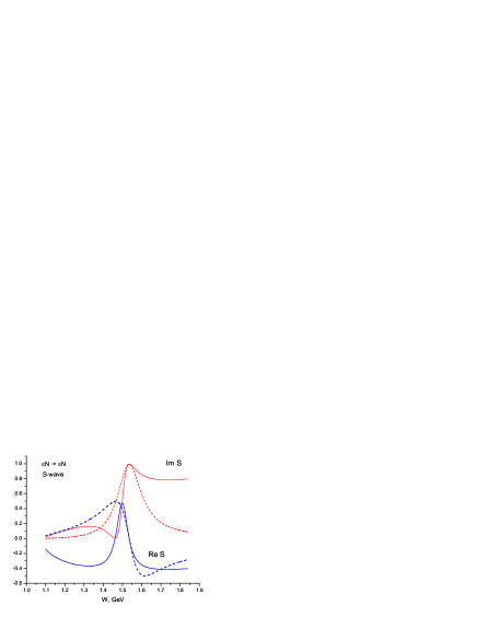
Figure 1: The results of calculations of $\pi N$ $s$-wave partial wave. Solid lines correspond to the real and imaginary parts of our partial amplitude (18), (20) in the single-channel approach with the parameters (33). Dashed lines correspond to our amplitudes, neglecting the mixing effect: $\Sigma_{12}=\Sigma_{21}=0$. All variants of amplitudes satisfy the single-channel unitary condition $\operatorname{\mathrm{Im}}S=\lvert S\rvert^{2}$.

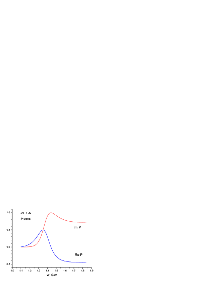
Figure 2: The real and imaginary parts of $\pi N$ partial $p$-wave. Notations are the same as in Fig. 1. For $p$-wave the solid and dashed lines coincide with each other.

It turns out that the discussed OPF-mixing leads to noticeable effects only in $s$-wave, while its influence in $p$-wave is much less and does not seen at graphics. This feature is explained by the values of the coupling constants in (33) $\lvert g_{2,\pi}\rvert\ll\lvert g_{1,\pi}\rvert$ and may be seen at qualitative level from the tree amplitudes (19), (21). Since we have normalized the coupling constants on the resonance width, inequality between the coupling constants is a consequence of the inequality between the $s$- and $p$-wave phase volumes.

We see that the discussed mixing effect generate the (unitary) interference picture “resonance + background” in the $s$-wave. In this case the $s$-wave background contribution originates from the $p$-wave resonance and gives the negative contribution to $s$-wave phase shift. This fact can be seen from Fig. 1 and from eq. (18).

Fig. 3 demonstrates the results of partial wave analysis Arn06 for lowest $\pi N$ amplitudes with isospin $I=1/2$. The discussed effect leads to hard correlation between pair of partial waves. From physical point of view the most interesting is the pair of waves $S_{11},P_{11}$; recall that in the $J^{P}=1/2^{+}$ sector there exist up to now the problems of physical interpretation of the observed states and their correspondence with quark models, see e.g. discussions in Cap00 ; Kre00 ; Sar08 ; Ces08 . But this pair of partial waves is not the simplest place for identification of the discussed OPF-mixing effect. The reasons are the old problem with Roper resonance (non-standard form of $1/2^{+}$ state) and the existence of several states in $1/2^{-}$ channel.

But if to look at the partial waves $P_{13},D_{13}$, where resonances $3/2^{\pm}$ are produced, here we observe the more evident situation, which is qualitatively consistent with our expectations, shown at Figs. 1, 2. Namely: in the $d$-wave we see a single resonance, whereas in the $p$-wave there is a visible interference of resonance with a background. Moreover, in accordance with our expectations for interference picture, the background in the $p$-wave is evidently negative – see Fig. 3. So this pair of partial waves $P_{13},D_{13}$ looks as a most suitable place for identification of the discussed mixing effect.

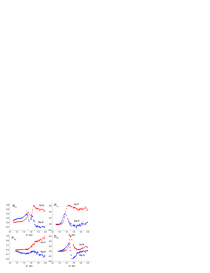
Figure 3: The results of partial wave analysis Arn06 for $\pi N$ scattering amplitudes with isospin $I=1/2$ (current solution). Partial waves satisfy the unitary condition $\operatorname{\mathrm{Im}}T=\lvert T\rvert^{2}+(1-\eta^{2})/4$.

V OPF-mixing for baryons $3/2^{\pm}$

The above discussion was devoted to mixing of two Dirac fields of opposite parities, the same effect arises for vector-spinor fields $\Psi^{\mu}$, which describe the spin-3/2 particles. We want to obtain the hadron partial amplitudes, which take into account the discussed effect, and to use them for description of results of $\pi N$ partial wave analysis.

The details of calculations of the spin-3/2 baryons production are given in the appendix A. Here we present only the results of calculations: the hadron partial amplitudes in two-channel ($\pi N$, $\eta N$) approach (compare them with spin-1/2 case (18), (20)).

$p$-wave amplitudes ($J^{P}={3/2}^{+}$) have the form:

$$\begin{split}f_{p,+}(\pi N\rightarrow\pi N)&=\lvert\mathbf{p}_{\pi}\rvert^{2}\frac{(E_{1}+m)}{24\pi W\Delta_{2}}\Big{[}g^{2}_{1,\pi}(W-m_{2}-\Sigma^{1}_{22})-g^{2}_{2,\pi}(-W-m_{1}-\Sigma^{2}_{11})+\\ &+\mathrm{i}\,g_{1,\pi}g_{2,\pi}(\Sigma^{3}_{21}+\Sigma^{4}_{12})\Big{]},\\ f_{p,+}(\pi N\rightarrow\eta N)&=\lvert\mathbf{p}_{\pi}\rvert\lvert\mathbf{p}_{\eta}\rvert\frac{\sqrt{(E_{1}+m)(E_{2}+m)}}{24\pi W\Delta_{2}}\Big{[}g_{1,\pi}g_{1,\eta}(W-m_{2}-\Sigma^{1}_{22})-\\ &-g_{2,\pi}g_{2,\eta}(-W-m_{1}-\Sigma^{2}_{11})+\mathrm{i}\,g_{1,\pi}g_{2,\eta}\Sigma^{4}_{12}+\mathrm{i}\,g_{2,\pi}g_{1,\eta}\Sigma^{3}_{21}\Big{]},\\ f_{p,+}(\eta N\rightarrow\eta N)&=\lvert\mathbf{p}_{\eta}\rvert^{2}\frac{(E_{2}+m)}{24\pi W\Delta_{2}}\Big{[}g^{2}_{1,\eta}(W-m_{2}-\Sigma^{1}_{22})-g^{2}_{2,\eta}(-W-m_{1}-\Sigma^{2}_{11})+\\ &+\mathrm{i}\,g_{1,\eta}g_{2,\eta}(\Sigma^{3}_{21}+\Sigma^{4}_{12})\Big{]},\\ \Delta_{2}&=\big{(}-W-m_{1}-\Sigma^{2}_{11}\big{)}\big{(}W-m_{2}-\Sigma^{1}_{22}\big{)}-\Sigma^{4}_{12}\Sigma^{3}_{21}.\end{split}$$ (34)

$d$-wave amplitudes ($J^{P}={3/2}^{-}$):

$$\begin{split}f_{d,-}(\pi N\rightarrow\pi N)&=\lvert\mathbf{p}_{\pi}\rvert^{2}\frac{(E_{1}-m)}{24\pi W\Delta_{1}}\Big{[}-g^{2}_{1,\pi}(-W-m_{2}-\Sigma^{2}_{22})+g^{2}_{2,\pi}(W-m_{1}-\Sigma^{1}_{11})-\\ &-\mathrm{i}\,g_{1,\pi}g_{2,\pi}(\Sigma^{4}_{21}+\Sigma^{3}_{12})\Big{]},\\ f_{d,-}(\pi N\rightarrow\eta N)&=\lvert\mathbf{p}_{\pi}\rvert\lvert\mathbf{p}_{\eta}\rvert\frac{\sqrt{(E_{1}-m)(E_{2}-m)}}{24\pi W\Delta_{1}}\Big{[}-g_{1,\pi}g_{1,\eta}(-W-m_{2}-\Sigma^{2}_{22})+\\ &+g_{2,\pi}g_{2,\eta}(W-m_{1}-\Sigma^{1}_{11})-\mathrm{i}\,g_{1,\pi}g_{2,\eta}\Sigma^{3}_{12}-\mathrm{i}\,g_{2,\pi}g_{1,\eta}\Sigma^{4}_{21}\Big{]},\\ f_{d,-}(\eta N\rightarrow\eta N)&=\lvert\mathbf{p}_{\eta}\rvert^{2}\frac{(E_{2}-m)}{24\pi W\Delta_{1}}\Big{[}-g^{2}_{1,\eta}(-W-m_{2}-\Sigma^{2}_{22})+g^{2}_{2,\eta}(W-m_{1}-\Sigma^{1}_{11})-\\ &-\mathrm{i}\,g_{1,\eta}g_{2,\eta}(\Sigma^{4}_{21}+\Sigma^{3}_{12})\Big{]},\\ \Delta_{1}&=\big{(}W-m_{1}-\Sigma^{1}_{11}\big{)}\big{(}-W-m_{2}-\Sigma^{2}_{22}\big{)}-\Sigma^{3}_{12}\Sigma^{4}_{21}.\end{split}$$ (35)

where $E_{1}$ and $E_{2}$ are nucleon energies for $\pi N$ and $\eta N$ states respectively.

The obtained $p$ and $d$ partial amplitudes satisfy the two-channel unitary condition (22).

Besides, we should take into account the $W$-dependent form-factor in a vertex (the so called centrifugal barrier factor). There is no common opinion in literature concerning its form, we take it in two-parameter form:

$$g\rightarrow g\cdot F(W^{2})=g\cdot\dfrac{1+aM^{2}+bM^{4}}{1+aW^{2}+bW^{4}}.$$ (36)

The partial amplitudes (34), (35), which take into account the OPF-mixing, are written in two-channel approach. But in fact in considered region of energy $W<2$ GeV there exist at least five open channels, the most essential are the $(\pi\pi)_{S}N$ and $\pi\Delta$ channels. In this situation we follow the way suggested in Bat95 ; Cec08 ; Ces08 : we restrict ourselves by the three-channel approach ($\pi N$, $\eta N$ and $\sigma N$). As for third channel ($\sigma N=\pi\pi N$), it is considered as some “effective” channel and its threshold may be a free parameter in a fit.

Three-channel amplitudes may be obtained from the formulae (50), (51) in appendix A, but they are rather cumbersome so we did not write down them. For our local purpose of the description of $\pi N\to\pi N$ amplitudes, it is sufficient to use formulae (34), (35). The only difference will appear in the self-energy, where we should add the third channel in the similar manner. We use the same procedure of loop renormalization as for spin $1/2$, see (25).

First of all let’s try to describe the ${P_{13}}$, ${D_{13}}$ separately. We found that, in accordance with our estimates for spin-1/2 case, the OPF-mixing is more essential for lowest $l$ wave ${P_{13}}$.

Results of $D_{13}$ fitting by formulae (35) in two-channel ($\pi N$, $\sigma N$) approach are shown at Fig. 4. We restricted the energy interval by $W<1.7$ GeV since at higher energy there appears some additional smooth contribution — it is seen well from $1-\eta^{2}$ behaviour. As for mass of “effective” $\sigma$-meson, fit leads to rather low value $m_{\sigma}\leq 0.3$ GeV. From other side, the d-wave threshold generates rather smooth contribution in amplitude and is defined badly from data. So we fix it by $m_{\sigma}=280$ MeV in the following.

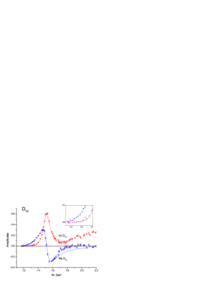
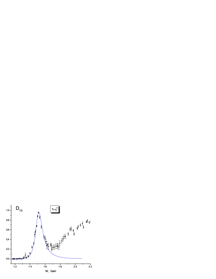
Figure 4: Left: $D_{13}$ partial wave of $\pi N$ scattering Arn06 and results of fit by our formulae with $\pi N$ and $\sigma N$ channels ($W<1.7$ GeV). Right: inelasticity from PWA Arn06 and our curve, corresponding to left panel.

Fit of real and imaginary parts of $D_{13}$ gives:

$$m_{1}=1.5161\pm 0.0005\,\text{GeV},\quad g_{1,\pi}=20.23\pm 0.10\,\text{GeV},\quad g_{1,\sigma}=21.60\pm 0.25\,\text{GeV},\\ \chi^{2}/\text{DOF}=213/59.$$ (37)

Parameters of form-factor from $D_{13}$ wave:

$$a=-1.005\pm 0.009\,\text{GeV}^{-2},\quad b=0.434\pm 0.021\,\text{GeV}^{-4}$$ (38)

Now we can describe $P_{13}$ at fixed parameters (37) of $D_{13}$ resonance. Results are shown at Fig. 5.

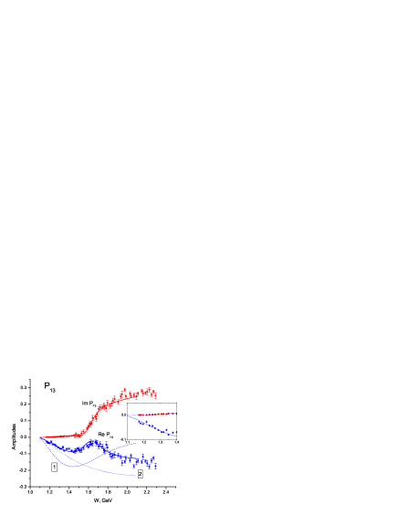
Figure 5: $P_{13}$ partial wave of $\pi N$ scattering Arn06 and results of fit by our formulae with $\pi N$ and $\sigma N$ channels ($W<2.0$ GeV). Parameters of $D_{13}$ resonance are fixed by (37). Curves 1 and 2 show the real part of background contribution from $D_{13}$ resonance ($g_{2,\pi}=g_{2,\sigma}=0$) with form-factors (38) and (40). Right: inelasticity from PWA Arn06 and our curve, corresponding to left panel.

$$m_{2}=1.721\pm 0.005\,\text{GeV},\quad g_{2,\pi}=3.73\pm 0.10\,\text{GeV},\quad g_{2,\sigma}=9.23\pm 0.25\,\text{GeV},\\ \chi^{2}/\text{DOF}=210/91.$$ (39)

Parameters of form-factor from $P_{13}$ wave:

$$a=1.51\pm 0.30\,\text{GeV}^{-2},\quad b=0.001\pm 0.017\,\text{GeV}^{-4}$$ (40)

We observe that both fits are consistent with each other in parameters of resonances, except for the vertex form-factor. The obtained parameters do not contradict to values of masses and branching ratios of $D_{13}(1520)$, $P_{13}(1720)$ in RPP tables RPP .

As for $\eta N$ channel: PWA results for $P_{13}$ wave does not require this coupling. For $D_{13}$ situation is unstable: inclusion of this coupling leads to unphysical big coupling constants. But close inspection shows that this is effect of another threshold with higher mass. So we will restrict ourselves by the two-channel approach.

Figs. 4, 5 demonstrate that fit of $D_{13}$ and $D_{13}$ separately leads to rather good quality of description. As for joint fit – it gives only qualitative description, as it seen from Fig.6. For better quality it needs “fine tuning”, first of all it should include:

• More accurate description of $(\pi\pi)N$ channel;

• Account of smooth contribution in $D_{13}$ wave – see Fig. 4;

• Better understanding of role and properties of the vertex form-factor. The observed disagreement may be related with above items.

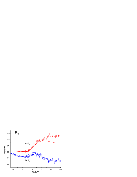
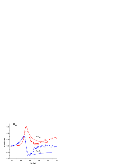
Figure 6: Example of joint description of $P_{13}$ (W < 2.0 GeV) and $D_{13}$ ($W<1.6$ GeV) partial waves by our formulae with OPF-mixing in two-channel approach. In this case $\chi^{2}/\text{DOF}=1220/139$.

Thus we can see that the considered mixing of the opposite parities fermion fields leads to the sizeable effects for baryon production and may be identified in production of baryon resonances $3/2^{\pm}$ in $\pi N$ scattering.

VI Conclusion

In present paper we have analyzed the mixing effect, specific for fermions, when two fermion fields of opposite parities are mixed at loop level. For fermions it is possibly even if the parity is conserved in a vertex. As a result we have a matrix propagator of unusual form (14), which contains $\gamma^{5}$ contributions. But since parity is conserved in vertexes, the $\gamma^{5}$ matrix disappears after multiplication by the vertexes, and we get the amplitudes containing the resonance and background contributions. Note that as a result of solving the Dyson–Schwinger equations we automatically obtain the unitary amplitudes.

The derived amplitudes resemble in structure the analytical $K$-matrix. The most significant difference is the presence of poles both of positive and negative energies in our amplitudes.

If to say about resonance phenomenology, we have a pair of partial waves with strongly correlated parameters, namely, the resonance in one partial wave is connected with background contribution in another wave. The discussed effect is most essential for partial wave with smaller orbital momentum $l$, thit is a consequence of inequality of phase volumes for different $l$.

As for manifestation of this effect in $\pi N$ scattering, the most simple physical example is connected with production of spin-$3/2$ resonances of opposite parities and isospin $I=1/2$. We used the obtained amplitudes for description of two $\pi N$ partial waves $\mathsf{P_{13}}$ and $\mathsf{D_{13}}$. We can conclude that the discussed effect reproduces naturally all the observed features of these partial waves but the joint description of these partial waves needs fine tuning of their properties.

We suppose that the most interesting application of this effect is related with the problem of Roper resonance $N(1440)$, $1/2^{+}$. Recall that for these quantum numbers there are still problems of physical interpretation of the baryon states and their comparison with quark models. The effect of OPF-mixing in this sector takes a more complicated form because of presence of several states $1/2^{-}$ (see Fig. 3) and non-standard form of the Roper resonance $1/2^{+}$. But the above mentioned strong correlation between two partial waves gives new possibilities for studying the properties of $N(1440)$.

Acknowledgements

This work was supported in part by the program “Development of Scientific Potential in Higher Schools” (project 2.2.1.1/1483, 2.1.1/1539) and by the Russian Foundation for Basic Research (project No. 09-02-00749).

Appendix A Amplitudes of production of spin-$3/2$ resonances

Let us write down the phenomenological Lagrangians of interaction of spin $3/2$ particles with $\pi N$ system.

For $J^{P}=3/2^{+}$ we have:

$$\mathscr{L}=g_{R,\pi}\bar{\Psi}\vphantom{\Psi}_{\mu}(x)\Psi(x)\cdot\partial_{\nu}\phi(x)+\text{h.c.}.$$ (41)

For $J^{P}=3/2^{-}$:

$$\mathscr{L}=ig_{R,\pi}\bar{\Psi}\vphantom{\Psi}_{\mu}(x)\gamma^{5}\Psi(x)\cdot\partial_{\nu}\phi(x)+\text{h.c.}.$$ (42)

Here $\Psi_{\mu}$ is the vector-spinor Rarita-Schwinger field, isotopical indices are omitted.

We are interested in the resonance contribution (the term of the leading spin $s=3/2$ in this diagram).

Propagator of Rarita-Schwinger field has the form (see more in Kal06 ; Kal04 ):

$$\begin{split}G^{\mu\nu}(p)&=\mathcal{P}^{\mu\nu}_{1}\cdot\bar{G}_{1}(W)+\mathcal{P}^{\mu\nu}_{2}\cdot\bar{G}_{2}(W)+\text{($s=1/2$ contributions)},\end{split}$$ (43)

where the basis elements are

$$\mathcal{P}^{\mu\nu}_{1}=\Lambda^{+}P^{\mu\nu}_{3/2},\quad\mathcal{P}^{\mu\nu}_{2}=\Lambda^{-}P^{\mu\nu}_{3/2}.$$ (44)

The operator $P_{3/2}$ looks like Pvn :

$$P_{3/2}^{\mu\nu}=g^{\mu\nu}-n_{1}^{\mu}n_{1}^{\nu}-n_{2}^{\mu}n_{2}^{\nu},$$ (45)

where we have introduced the unit "vectors" orthogonal to each other:

$$n_{1}^{\mu}=\frac{1}{\sqrt{3}p^{2}}(-p^{\mu}+\gamma^{\mu}\hat{p})\hat{p},\quad n_{2}^{\mu}=\frac{p^{\mu}}{\sqrt{p^{2}}},\quad(n_{i}\cdot n_{j})=\delta_{ij}.$$ (46)

In the presence of parity violation or when considering the OPF-mixing the basis in the sector $s=3/2$ must be supplemented by elements containing $\gamma^{5}$:

$$\begin{split}Q^{\mu\nu}_{1}&=\mathcal{P}^{\mu\nu}_{1},\quad\quad Q^{\mu\nu}_{2}=\mathcal{P}^{\mu\nu}_{2},\\ Q^{\mu\nu}_{3}&={\cal P}^{\mu\nu}_{1}\gamma^{5},\quad\quad Q^{\mu\nu}_{4}={\cal P}^{\mu\nu}_{2}\gamma^{5}.\\ \end{split}$$ (47)

Suppose we have two fields $\Psi^{\mu}$ of opposite parities. When taking into account OPF-mixing the dressed propagator has the following decomposition:

$$G^{\mu\nu}(p)=\sum_{M=1}^{4}Q^{\mu\nu}_{M}\cdot\bar{G}_{M}(W)+\text{($s=1/2$ contributions)},$$ (48)

where $\bar{G}_{M}(W)$ being dimension 2 matrices are solutions of the matrix Dyson–Schwinger equation.

Since the multiplicative properties of the operators $Q^{\mu\nu}_{M}$ are completely consistent with the properties of the spin-$1/2$ operators (see Table 1), the further calculations repeat $s=1/2$ ones. As a result the matrix propagator looks similar to spin-$1/2$ case (14).

Matrix amplitude has the form:

$$T=\bar{u}(p_{2},s_{2})Ru(p_{1},s_{1}),$$ (49)

where the matrix $R$ is constructed from the matrix of the propagator and vertex matrices:

$$R=-V^{T}\times\bigg{(}\sum_{M=1}^{4}k_{2}^{\mu}Q^{\mu\nu}_{M}k_{1}^{\nu}\cdot\bar{G}_{M}(W)\bigg{)}\times V.$$ (50)

The vertex matrix in two-channel approximation looks like

$$V=\begin{pmatrix}g_{1,\pi}\gamma^{5}&g_{1,\eta}\gamma^{5}\\ ig_{2,\pi}&ig_{2,\eta}\end{pmatrix}.$$ (51)

The self-energy

$$\Sigma^{\mu\nu}=-V\begin{pmatrix}\hat{\Sigma}^{\mu\nu}_{\pi}&0\\ 0&\hat{\Sigma}^{\mu\nu}_{\eta}\end{pmatrix}V^{T}+\text{subtraction},$$ (52)

is expressed through the standard loop function corresponding to one of the channels. For $\pi N$ channel this standard function has form:

$$\hat{\Sigma}^{\mu\nu}_{\pi}=-i\int\dfrac{d^{4}k}{(2\pi)^{4}}\dfrac{k^{\mu}k^{\nu}}{(\hat{p}-\hat{k}-m_{N})(k^{2}-m_{\pi}^{2})}=Q^{\mu\nu}_{1}\cdot\hat{\Sigma}^{1}_{\pi}+Q^{\mu\nu}_{2}\cdot\hat{\Sigma}^{2}_{\pi}+\text{($s=1/2$ contributions)},$$ (53)

and similarly for $\eta N$ the channel. An alternative decomposition of the loop is

$$\hat{\Sigma}^{\mu\nu}_{\pi}=(A_{\pi}(p^{2})+\hat{p}B_{\pi}(p^{2}))P_{3/2}^{\mu\nu}+\text{($s=1/2$ contributions)},$$ (54)

so that

$$\begin{split}\hat{\Sigma}^{1}_{\pi}(W)&=A_{\pi}(W^{2})+WB_{\pi}(W^{2}),\\ \hat{\Sigma}^{2}_{\pi}(W)&=A_{\pi}(W^{2})-WB_{\pi}(W^{2}).\end{split}$$ (55)

Imaginary parts are

$$\begin{split}\operatorname{\mathrm{Im}}A_{\pi}&=-\dfrac{\lvert\mathbf{p}_{\pi}\rvert^{3}m_{N}}{24\pi W},\\ \operatorname{\mathrm{Im}}B_{\pi}&=-\dfrac{\lvert\mathbf{p}_{\pi}\rvert^{3}(W^{2}+m_{N}^{2}-m_{\pi}^{2})}{48\pi W^{3}},\end{split}$$ (56)

and hence

$$\begin{split}\operatorname{\mathrm{Im}}\hat{\Sigma}^{1}_{\pi}&=-\dfrac{\lvert\mathbf{p}_{\pi}\rvert^{3}(E_{1}+m_{N})}{24\pi W},\\ \operatorname{\mathrm{Im}}\hat{\Sigma}^{2}_{\pi}&=\dfrac{\lvert\mathbf{p}_{\pi}\rvert^{3}(E_{1}-m_{N})}{24\pi W}.\end{split}$$ (57)

Here $\mathbf{p}_{\pi}$, $E_{1}$ are momentum and energy in the CMS of $\pi N$ system.

Let us express the self-energy contributions (for two channels, without subtraction polynomials) in terms of the standard loop functions:

$$\begin{split}\Sigma^{1}_{11}(W)&=-g_{1,\pi}\hat{\Sigma}^{2}_{\pi}g_{1,\pi}-g_{1,\eta}\hat{\Sigma}^{2}_{\eta}g_{1,\eta},\\ \Sigma^{2}_{11}(W)&=-g_{1,\pi}\hat{\Sigma}^{1}_{\pi}g_{1,\pi}-g_{1,\eta}\hat{\Sigma}^{1}_{\eta}g_{1,\eta}=\Sigma^{1}_{11}(-W),\\ \Sigma^{3}_{21}(W)&=-ig_{2,\pi}\hat{\Sigma}^{1}_{\pi}g_{1,\pi}-ig_{2,\eta}\hat{\Sigma}^{1}_{\eta}g_{1,\eta},\\ \Sigma^{4}_{21}(W)&=-ig_{2,\pi}\hat{\Sigma}^{2}_{\pi}g_{1,\pi}-ig_{2\,eta}\hat{\Sigma}^{2}_{\eta}g_{1,\eta}=\Sigma^{3}_{21}(-W),\\ \Sigma^{3}_{12}(W)&=\Sigma^{4}_{21}(W),\\ \Sigma^{4}_{12}(W)&=\Sigma^{3}_{21}(W).\end{split}$$

Substituting all the necessary into (50) we obtain the partial waves (34), (35).

References

- (1) B. Pontecorvo. Sov.Phys. JETP 6 (1958) 429.
- (2) N.Cabibbo. Phys.Rev.Lett. 10 (1963) 531; M.Kobayashi and T.Maskawa. Prog.Theor.Phys. 49 (1973) 652.
- (3) M.Beuthe. Phys.Rep. 375 (2003) 105.
- (4) D.Espriu, J.Manzano and P.Talavera. Phys.Rev. D66 (2002) 076002.
- (5) M.Blasone and J.Palmer. Phys.Rev. D69 (2004) 057301.
- (6) B.Machet, V.A.Novikov and M.Vysotsky. Int.J.Mod.Phys. A20 (2005) 5399.
- (7) B.A.Kniehl and A.Sirlin. Phys.Rev. D74 (2006) 116003.
- (8) Q.Duret, B.Machet and M.Vysotsky. Eur.Phys.J. C61 (2009) 247.
- (9) A.E.Kaloshin and V.P.Lomov. Yad.Fiz. 69 (2006) 563.
- (10) A.E.Kaloshin and V.P.Lomov. Int.J.Mod.Phys. 19 (2004) 135.
- (11) M.O.Gonchar, A.E.Kaloshin and V.P.Lomov. Int.J.Mod.Phys. V22 (2007) 24.
- (12) R.E.Cutkosky et al. Phys.Rev. D20 (1979) 2839.
- (13) R.Koch. Z.Phys. C29 (1985) 597.
- (14) G.Höhler. Newsletters 9 (1993) 1.
- (15) R.A.Arndt et al. Phys.Rev. C52 (1995) 2120.
- (16) R.A.Arndt et al. Phys.Rev. C74 (2006) 045205; http://gwdac.phys.gwu.edu
- (17) K.I.Aoki et al. Prog.Theor.Phys.Suppl. 73 (1982) 1.
- (18) A.Denner. Fortschr.Phys. 41 (1993) 307.
- (19) S.W.MacDowell. Phys.Rev.116 (1959) 774.
- (20) O.Babelon et al. Nucl.Phys. 113 (1976) 445.
- (21) R.A.Arndt, J.M.Ford and L.D.Roper. Phys.Rev. D32 (1985) 1085.
- (22) S.Capstick and W.Roberts. Prog.Part.Nucl.Phys 45 (2000) 241.
- (23) O.Krehl et al. Phys.Rev. C62 (2000) 025207.
- (24) A.V.Sarantsev et al. Phys.Lett. B659 (2008) 94.
- (25) S.Ceci, A.Švars and B.Zauner. Eur.Phys.J. C58 (2008) 47.
- (26) M.Batinic et al. Phys.Rev. C51 (1995) 2310.
- (27) S.Ceci at al. Phys.Rev. D77 (2008) 116007.
- (28) K. Nakamura et al. (Particle Data Group) J. Phys. G 37 (2010) 075021.
- (29) P.van Nieuwenhuizen. Phys.Rep.68 (1981) 189.