The 2D AKLT state on the honeycomb lattice is a universal resource for quantum computation

Abstract

Universal quantum computation can be achieved by simply performing single-qubit measurements on a highly entangled resource state. Resource states can arise from ground states of carefully designed two-body interacting Hamiltonians. This opens up an appealing possibility of creating them by cooling. The family of Affleck-Kennedy-Lieb-Tasaki (AKLT) states are the ground states of particularly simple Hamiltonians with high symmetry, and their potential use in quantum computation gives rise to a new research direction. Expanding on our prior work [T.-C. Wei, I. Affleck, and R. Raussendorf, Phys. Rev. Lett. 106, 070501 (2011)], we give detailed analysis to explain why the spin-3/2 AKLT state on a two-dimensional honeycomb lattice is a universal resource for measurement-based quantum computation. Along the way, we also provide an alternative proof that the 1D spin-1 AKLT state can be used to simulate arbitrary one-qubit unitary gates. Moreover, we connect the quantum computational universality of 2D random graph states to their percolation property and show that these states whose graphs are in the supercritical (i.e. percolated) phase are also universal resources for measurement-based quantum computation.

I Introduction

The rules of quantum mechanics appear to perform certain tasks much more efficiently than those of classical mechanics. The most celebrated example is the factoring of a large integer by Shor’s quantum algorithm Shor that offers exponential speedup over existing classical algorithms. Quantum computers that implement generic quantum algorithms can take form in various computational models, such as the standard circuit model NielsenChuang00 , adiabatic quantum computer AQC ; AQC2 , and quantum walk Childs , all of which proceed via the important feature of quantum mechanics—the unitary evolution.

A different but equally powerful framework is the measurement-based quantum computation GottesmanChuang ; NielsenLeungChilds ; Oneway . A particular computational model within this class is One-Way quantum computation Oneway which we subsequently denote by MBQC. It proceeds by single-qubit measurements alone on a highly entangled initial resource state Oneway ; Oneway2 ; RaussendorfWei12 . For MBQC, resource states that allow universal quantum computation turns out to be very rare Gross1 , but examples do exist Cluster ; Gross ; Verstraete ; Cai . The first identified universal resource state is the 2D cluster state on the square lattice Oneway ; Cluster . It was also shown that 2D cluster states defined on regular lattices, such as triangular, hexagonal and Kagomé, are also universal resources Universal . Cluster states and related graph states can be created by the Ising interaction from unentangled states Cluster and they have been created with cold atoms in optical lattices coldatom . However, they do not arise as unique ground states of two-body interacting Hamiltonians Nielsen , although they can be an approximate unique ground state BartlettRudolph . However, by going beyond qubit systems and by careful design of Hamiltonians, a few quantum states have been found that are both unique ground states and universal for MBQC Chen ; Cai10 ; WeiRaussendorfKwek11 ; LiEtAl . This opens up an alternative possibility of creating universal resource states by cooling the systems.

Independently of the development on quantum computation, Affleck, Kennedy, Lieb and Tasaki (AKLT) constructed a family of states that were ground states of isotropic antiferromagnet-like Hamiltonians AKLT ; AKLT2 ; AKLT3 . In any dimension, AKLT states are ground states of particularly simple Hamiltonians which only have nearest-neighbor two-body interactions, are rotationally invariant in spin space and shares all spatial symmetries of the underlying lattice. In particular, AKLT provided an explicit example of a one-dimensional spin-1 chain that has a finite spectral gap above the ground state, supporting Haldane’s conjecture on integer spin chains with spin rotation symmetry Haldane . These valence-bond states turned out to be the first examples of matrix product states (MPS) MPS and projected entangled pairs states (PEPS) Verstraete ; PEPS . The use of MPS and PEPS also gives rise to a new perspective on MQBC Verstraete ; Gross . In particular, it was recently discovered that the one-dimensional spin-1 AKLT state AKLT ; AKLT2 can serve as resources for restricted computations Gross ; Brennen , i.e., implementation of arbitrary one-qubit rotations. The discovery of the resourcefulness of AKLT states creates additional avenues for its experimental realization Resch , and has instilled novel concepts in MBQC, such as the renormalization group and the holographic principle Bartlett ; Miyake . However, to achieve universal quantum computation within the measured-based architecture a two-dimensional structure is needed.

In Ref. Cai10 , Cai et al. considered stacking up 1D AKLT quasichains to form a 2D structure. Their construction showed that the resulting state, even though it is longer an AKLT state, can provide universal quantum computation. Later independently by us WeiAffleckRaussendorf11 and by Miayke Miyake10 , it was shown that indeed the 2D AKLT state on the honeycomb lattice provides a universal resource for MQBC. Here, expanding on our prior work WeiAffleckRaussendorf11 , we provide an alternative proof that the 1D spin-1 AKLT state can be used to simulate arbitrary one-qubit unitary gates, and generalize the method and give detailed analysis to the proof that the spin-3/2 AKLT state on a two-dimensional honeycomb lattice is a universal resource for measurement-based quantum computation. We do this by showing that a 2D cluster state can be distilled by local operations. Along the way, we have connected the quantum computational universality of 2D random graph states to their percolation property. We note that extension of our approach using Positive Operator Valued Measure (POVM) and percolation consideration to computational universality have been successfully applied to a deformed AKLT model in Ref. DarmawanBrennenBartlett .

The structure of the present paper is as follows. In Sec. II we discuss how to locally convert a 1D AKLT to a 1D cluster state. In Sec. III we outline and illustrate the method of how to locally convert the 2D AKLT state to a random graph state. We then give the general proof in Sec IV. In Sec. V we show the quantum computational universality of these graph states is related to the percolation of the graph and show how to convert these graph states to a 2D cluster state on a square lattice. We support our assertion with Monte Carlo simulations in Sec. VI and conclude in Sec. VII. In the Appendices, we use a different approach to obtain the probability of getting any POVM outcomes.

II One dimension

We begin by investigating the 1D AKLT state and how it can be locally converted to a 1D cluster state. By doing so, we have thus proved the equivalence of the capability to simulate one-qubit unitary gates for both types of states. Many of the methods developed in this section can be extended to the more interesting case of 2D AKLT state on the honeycomb lattice.

II.1 1D spin-1 AKLT state and 1D cluster state

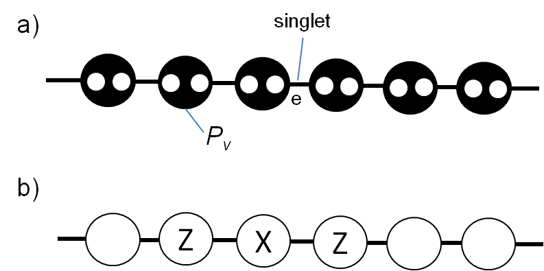
Figure 1: The 1D AKLT state (a) and the 1D cluster state (b).

The 1D AKLT state AKLT can be understood by using the valence-bond-solid (VBS) picture, as illustrated in Fig. 1a. (1) First one regards a spin-1 particle at each site as consisting of two virtual spin-1/2 particles (qubits), each of which forms a singlet with the virtual qubit on the neighboring site: $|\phi\rangle_{e}\equiv|01\rangle_{e}-|10\rangle_{e}$, where the normalization is omitted, $|0\rangle\equiv|\uparrow\rangle$ and $|1\rangle\equiv|\downarrow\rangle$ are eigenstates of Pauli $\sigma_{z}$, and $e$ denotes the edge that links the two virtual qubits. (2) A local projection is then made at every site that maps the state of the two virtual qubits to their symmetric subspace, which is then identified as the Hilbert space of spin-1 particle:

$$\hat{P}_{v}=|S_{z}=1\rangle\langle 00|+|S_{z}=-1\rangle\langle 11|+|S_{z}=0\rangle\langle\psi^{+}|,$$ (1)

$$|\psi^{+}\rangle\equiv\frac{1}{\sqrt{2}}(|01\rangle+|10\rangle),$$ (2)

where $|S_{z}=\pm 1,0\rangle$ are the three $S=1$ angular momentum eigenstates: $\hat{S}_{z}|S_{z}\rangle=S_{z}|S_{z}\rangle$. For convenience we shall take the periodic boundary condition, so that the last site of the 1D chain is actually connected to the first site of the chain. Open boundary condition can be dealt with by attaching qubits at the ends. The 1D AKLT is therefore given by

$$|\Phi^{(1D)}_{\rm AKLT}\rangle\equiv\bigotimes_{v}\hat{P}_{v}\bigotimes_{e}|\phi\rangle_{e},$$ (3)

which is the unique ground state of the following spin-isotropic Hamiltonian with a finite gap AKLT ; AKLT2 :

$$H_{\rm AKLT}^{S=1}=\sum_{v}\Big{[}\vec{S}_{v}\cdot\vec{S}_{v+1}+\frac{1}{3}(\vec{S}_{v}\cdot\vec{S}_{v+1})^{2}+\frac{2}{3}\Big{]},$$ (4)

where $\vec{S}_{v}$ denotes the vector of the spin operator at site $v$. This AKLT model provided strong evidence in support of the Haldane’s conjecture Haldane .

On the other hand, the 1D cluster state $|{\cal C}_{1D}\rangle$ also can be understood similarly by projecting virtual entangled pairs to physical spins, known as projected entangled pairs states (PEPS) PEPS , where the virtual entangled pair is replaced by $|\phi_{H}\rangle_{e}\equiv|00\rangle+|01\rangle+|10\rangle-|11\rangle$ and the local projection is given by $\hat{P}_{v}^{{\cal C}}\equiv|0\rangle\langle 00|+|1\rangle\langle 11|$, giving rise to

$$|{\cal C}^{(1D)}\rangle\equiv\bigotimes_{v}\hat{P}_{v}^{{\cal C}}\bigotimes_{e}|\phi_{H}\rangle_{e}.$$ (5)

However, for our purpose, it will be useful to define equivalently the cluster state as the common eigenstate of the following operators:

$$Z_{v-1}X_{v}Z_{v+1}|{\cal C}^{(1D)}\rangle=|{\cal C}^{(1D)}\rangle,$$ (6)

for all sites $v$, where $v\pm 1$ are the two neighboring sites of $v$ on the chain. Note that for convenience we denote the three Pauli matrices by $X\equiv\sigma_{x}$, $Y\equiv\sigma_{y}$ and $Z\equiv\sigma_{z}$, and use the two notations interchangeably. Moreover, the choice of “+1” or “-1” eigenvalue is arbitrary, as the resulting states are related by local unitary transformation. The 1D cluster state can be used to simulate one-qubit unitary operation on one qubit and is the basic ingredient in MBQC Oneway .

In fact, the 1D AKLT state has been shown to be able to simulate one-qubit unitary operation as the 1D cluster state Gross ; Brennen ; Miyake by explicitly constructing one-qubit universal gates. It has also been realized that the spin-1 AKLT state can actually be converted, via local operations, to the 1D spin-1/2 cluster state with a random length Chen10 . In the following section, we provide an alternative method for the reduction of the 1D AKLT state to a 1D cluster state. This method will then be generalized later for the reduction of the 2D AKLT state.

II.2 Reducing 1D AKLT state to a 1D cluster state

As spin-1 Hilbert space is of dimensionality three, in order to convert to dimensionality two of a qubit, a projection or a generalized measurement is needed. In the mapping $\hat{P}_{v}$ in Eq. (1), there is a two-dimensional subspace spanned by $|S=1,S_{z}=1\rangle$ and $|S=1,S_{z}=-1\rangle$ or equivalently by the two virtual qubits $|00\rangle$ and $|11\rangle$. One can therefore consider

$$F_{z}=(|S_{z}=1\rangle\langle S_{z}=1|+|S_{z}=-1\rangle\langle S_{z}=-1|)/\sqrt{2}$$ (7)

as a projection that preserves a two-dimensional subspace, where we suppress the label $S=1$. However, what happens if the projection is not successful and it ends up in the subspace orthogonal to that spanned by $|S_{z}=1\rangle$ and $|S_{z}=-1\rangle$? To solve this “leakage” problem, one takes advantage of the rotation symmetry and adds two more projections:

$$F_{x}=(|S_{x}=1\rangle\langle S_{x}=1|+|S_{x}=-1\rangle\langle S_{x}=-1|)/\sqrt{2},$$ (8)

$$F_{y}=(|S_{y}=1\rangle\langle S_{y}=1|+|S_{y}=-1\rangle\langle S_{y}=-1|)/\sqrt{2},$$ (9)

and notice the completeness relation in the spin-1 Hilbert space:

$$\sum_{\alpha=x,y,z}F^{\dagger}_{\alpha}F_{\alpha}=\openone_{S=1}.$$ (10)

The above $F$’s constitute the so-called generalized measurement or POVM, characterized by $\{F_{\alpha}^{\dagger}F_{\alpha}\}$. Their physical meaning is to define a two-dimensional subspace and to specify a preferred quantization axis $x$, $y$ or $z$. In principle, the POVM can be realized by a unitary transformation $U$ jointly on a spin-1 state, denoted by $|\psi\rangle$, and a meter state $|0\rangle_{m}$ such that

$$U|\psi\rangle|0\rangle_{m}=\sum_{\alpha}F_{\alpha}|\psi\rangle|\alpha\rangle_{m},$$ (11)

where for the meter states $\langle\alpha|\alpha^{\prime}\rangle=\delta_{\alpha,\alpha^{\prime}}$. A measurement on the meter state will result in a random outcome $\alpha$, for which the spin state is projected to $F_{\alpha}|\psi\rangle$ NielsenChuang00 .

Claim. We shall show that after performing the generalized measurement on all sites with $\{a_{v}\}$ denoting the measurement outcome the resulting state

$$|\psi(\{a_{v}\})\rangle\equiv\bigotimes_{v}F_{v,a_{v}}|\Phi^{(1D)}_{\rm AKLT}\rangle$$ (12)

is an “encoded” 1D cluster state.

In the following we shall make use of the equivalent representation of the AKLT state by the virtual qubits; see Eq. (1), e.g., $|S_{z}=1\rangle=|00\rangle$ and $|S_{z}=-1\rangle=|11\rangle$, where the r.h.s are two-qubit states. In this regard, we can think of $F$ operators in terms of two-qubit operators:

$$\tilde{F}_{z} = (|00\rangle\langle 00|+|11\rangle\langle 11|)/\sqrt{2},$$ (13a)

$$\tilde{F}_{x} = (|++\rangle\langle++|+|--\rangle\langle--|)/\sqrt{2},$$ (13b)

$$\tilde{F}_{y} = (|i,i\rangle\langle i,i|+|-i,-i\rangle\langle-i,-i|)/\sqrt{2},$$ (13c)

where $|\pm\rangle$ satisfy $\sigma_{x}|\pm\rangle=\pm|\pm\rangle$ and $|\pm i\rangle$ satisfy $\sigma_{y}|\pm i\rangle=\pm|\pm i\rangle$. Thus, in terms of these $\tilde{F}$’s the post-measurement state (12) is simply given by

$$|\psi(\{a_{v}\})\rangle\equiv\bigotimes_{v}F_{v,a_{v}}\bigotimes_{e}|\phi\rangle_{e}.$$ (14)

Naturally as with $|S_{z}=\pm 1\rangle$, there is also the correspondence between the other two $S=1$ states and the two-qubit states in $x$ and $y$ bases: $|S_{x}=1\rangle=|++\rangle$, $|S_{x}=-1\rangle=|--\rangle$, $|S_{y}=1\rangle=|i,i\rangle$, and $|S_{y}=-1\rangle=|-i,-i\rangle$. The use of qubit enables us to take the advantage of the stabilizer formalism Stabilizer , even though its use is not essential.

First, let us explain the meaning of “encoding” used in the claim. Suppose two neighboring sites $u$ and $v$ have the same outcome $a=z$; see Fig. 2a. Then the two-dimensional subspaces at sites $u$ and $v$ are both spanned by $|00\rangle$ and $|11\rangle$. However, the singlet state between the two virtual qubits connecting $u$ and $v$ dictates that the appearance of the basis states are anti-correlated. For example, $|(00)_{u}\rangle$ at site $u$ cannot coexist with $|(00)_{v}\rangle$ at site $v$. There are only two possible basis states for the two sites $u$ and $v$: $|``0"\rangle\equiv|(00)_{u}(11)_{v}\rangle$ and $|``1"\rangle\equiv|(11)_{u}(00)_{v}\rangle$. These two states “encode” a logical qubit $\{|``0"\rangle,|``1"\rangle\}$. In terms of spin-1 notation, they are $|S_{z}=1,S_{z}=-1\rangle_{u,v}$ and $|S_{z}=-1,S_{z}=1\rangle_{uv}$, showing the antiferromagnetic properties of the AKLT state. From these two states, logical Z and X operators can be defined: $Z\equiv|``0"\rangle\langle``0"|-|``1"\rangle\langle``1"|$ and $X\equiv|``0"\rangle\langle``1"|+|``1"\rangle\langle``0"|$ (and thus the Pauli operator $Y=-iZX$ can be determined). In the same manner, for $k$ consecutive sites with the same outcome $a$, only one qubit is encoded by the $k$ physical spins with quantization axis being in the $a$-direction. We shall refer to these sites collectively as a domain. On the other hand, for two neighboring sites having different outcome $a_{u}\neq a_{v}$, the four combination $|S_{a_{u}}=\pm 1,S_{a_{v}}=\pm 1\rangle$ can appear and each site is effectively a qubit.

The above analysis can be expressed in terms of the stabilizer formalism. In the example that neighboring $u$ and $v$ share the same outcome $a=z$ (i.e., the domain consists of two sites $u$ and $v$), for the two virtual qubits of site $u$ (denoted by the $1$ and $2$) we have $\sigma_{z}^{[1]}\otimes\sigma_{z}^{[2]}\tilde{F}_{u,z}=\tilde{F}_{u,z}$. This means $\sigma_{z}^{[1]}\otimes\sigma_{z}^{[2]}|\psi(\{a_{v}\})\rangle=|\psi(\{a_{v}\})\rangle$. Similarly, for site $v$ (with two virtual qubits labeled as $3$ and $4$) we have $\sigma_{z}^{[3]}\otimes\sigma_{z}^{[3]}|\psi(\{a_{v}\})\rangle=|\psi(\{a_{v}\})\rangle$. However, because of the singlet between $2$ and $3$, we have $-\sigma_{z}^{[2]}\otimes\sigma_{z}^{[3]}|\psi(\{a_{v}\})\rangle=|\psi(\{a_{v}\})\rangle$. The above three operators $\{\sigma_{z}^{[1]}\otimes\sigma_{z}^{[2]},\sigma_{z}^{[3]}\otimes\sigma_{z}^{[4]},-\sigma_{z}^{[2]}\otimes\sigma_{z}^{[3]}\}$ are called the stabilizer generators and they define the logical qubit basis states: $|``0"\rangle\equiv|(00)_{u}(11)_{v}\rangle$ and $|``1"\rangle\equiv|(11)_{u}(00)_{v}\rangle$, as one can verify that they are the common eigenstates of these operators with eigenvalue $+1$. The stabilizer generators are effectively identity operators in the logical-qubit Hilbert space. To define the logical $Z$ operator, there are many equivalent choices: e.g., $\sigma_{z}^{[1]}$, $\sigma_{z}^{[2]}$, $-\sigma_{z}^{[3]}$ and $-\sigma_{z}^{[4]}$. Any of them can be taken to one another by multiplication of some combination of the stabilizer generators. To complete the logical qubit operators, the $X$ operator can be taken as $X\equiv\sigma_{x}^{[1]}\sigma_{x}^{[2]}\sigma_{x}^{[3]}\sigma_{x}^{[4]}$, which flips $|``0"\rangle$ to $|``1"\rangle$, and vice versa. Other outcomes can be dealt with in a similar way, and these are summarized in Table 1. Two important properties are that (i) each domain can contain more than one physical qubit and is only one logical qubit; (2) the qubit basis depends on the shared outcome of the POVM.

POVM outcome	$z$	$x$	$y$
stabilizer generator	$\lambda_{i}\lambda_{i+1}\sigma_{z}^{[i]}\sigma_{z}^{[i+1]}$	$\lambda_{i}\lambda_{i+1}\sigma_{x}^{[i]}\sigma_{x}^{[i+1]}$	$\lambda_{i}\lambda_{i+1}\sigma_{y}^{[i]}\sigma_{y}^{[i+1]}$
$\overline{X}$	$\bigotimes_{j=1}^{2|{\cal{C}}|}\sigma_{x}^{[j]}$	$\bigotimes_{j=1}^{2|{\cal{C}}|}\sigma_{z}^{[j]}$	$\bigotimes_{j=1}^{2|{\cal{C}}|}\sigma_{z}^{[j]}$
$\overline{Z}$	$\lambda_{i}\sigma_{z}^{[i]}$	$\lambda_{i}\sigma_{x}^{[i]}$	$\lambda_{i}\sigma_{y}^{[i]}$

Table 1: The dependence of stabilizers and encodings for the random graphs on the local POVM outcome in the case of 1D AKLT state. $|{\cal C}|$ denotes the total number of virtual qubits contained in a domain. In the first line, $i=1\,..\,2|{\cal{C}}|-1$, and in the third line $i=1\,..\,2|{\cal{C}}|$. One choice of the sign is $\lambda_{i}=1$ if the virtual qubit $i$ is on the odd number of sites (relative to, e.g., the left end) in the domain and $\lambda_{i}=-1$ otherwise.

We remark that even though a domain may contain two or more sites one can perform projective measurement on all but one site in the basis defined by $\{|S_{a}=1\rangle\pm|S_{a}=-1\rangle\}$, where $a$ is the label of the POVM outcome for the domain. The domain is then reduced to a single site but still preserves the same degree of entanglement with its neighbors.

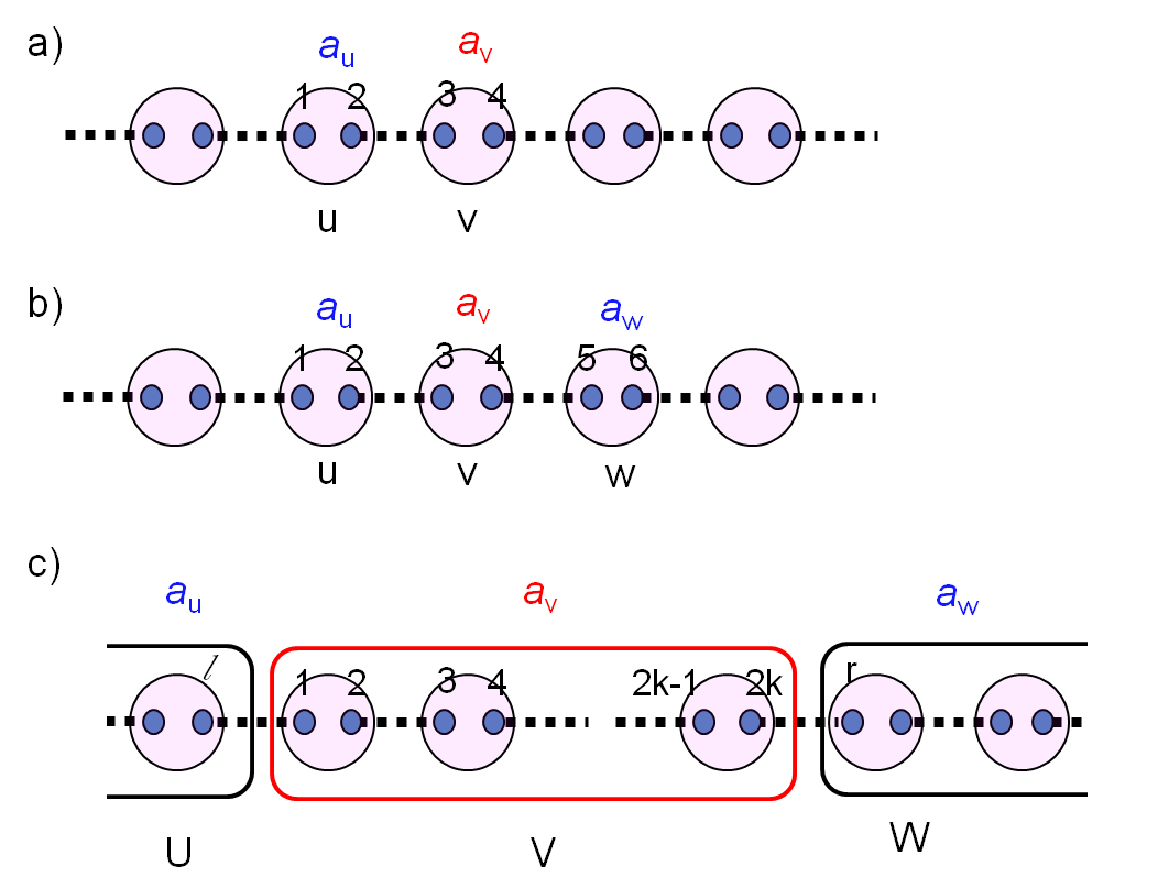
Figure 2: Illustration of (a) encoding and (b)& (c) stabilizer operator.

To show that the post-POVM state is an (encoded) cluster state, let us illustrate with the example shown in Fig. 2b. Let us label the three sites by $u$, $v$ and $w$ respectively. Suppose the POVM outcomes on these sites are $a_{u}=x$, $a_{v}=z$, and $a_{w}=x$, respectively. First note that $-\sigma_{x}^{[2]}\sigma_{x}^{[3]}$ commutes with $\tilde{F}_{u,x}$ and $-\sigma_{x}^{[4]}\sigma_{x}^{[5]}$ commutes with $\tilde{F}_{w,x}$. Note also that $-\sigma_{x}^{[2]}\sigma_{x}^{[3]}$ is a stabilizer operator of the singlet between $2$ and $3$, but it does not commute with $\tilde{F}_{v,z}$. Similarly, $-\sigma_{x}^{[4]}\sigma_{x}^{[5]}$ is a stabilizer operator of the singlet between $4$ and $5$, but it does not commute with $\tilde{F}_{v,z}$, either. However, if we multiply all the above operators, we obtain

$$K_{v}\equiv\sigma_{x}^{[2]}\sigma_{x}^{[3]}\sigma_{x}^{[4]}\sigma_{x}^{[5]}.$$ (15)

Because $\sigma_{x}^{[3]}\sigma_{x}^{[4]}$ commutes with $\tilde{F}_{v,z}$, due to the identity

$$\sigma_{x}\otimes\sigma_{x}(|00\rangle\langle 00|+|11\rangle\langle 11|)$$ (16)

$$= (|11\rangle\langle 00|+|00\rangle\langle 11|)$$

$$= (|00\rangle\langle 00|+|11\rangle\langle 11|)\,\sigma_{x}\otimes\sigma_{x},$$

$K_{v}$ is thus a stabilizer operator for the post-POVM state. In terms of logical Pauli operators $\overline{Z}_{u}\equiv\sigma_{x}^{[2]}$ , $\overline{Z}_{w}\equiv\sigma_{x}^{[5]}$, $\overline{X}_{v}\equiv\sigma_{x}^{[3]}\sigma_{x}^{[4]}$, we arrive at the stabilizer operator $K_{V}=\overline{Z}_{U}\overline{X}_{V}\overline{Z}_{W}$. This is the stabilizer operator defining a linear cluster state; see Eq. (6).

As a further illustration, let us consider the same three sites in Fig. 2b but with $a_{u}=x$, $a_{v}=z$, and $a_{w}=y$, i.e., the last site has a different outcome $a_{w}=y$ than the above example. Because of this, one now considers $-\sigma_{y}^{[4]}\sigma_{y}^{[5]}$ instead of $-\sigma_{x}^{[4]}\sigma_{x}^{[5]}$ and can show that the following operator is a stabilizer generator:

$$K_{V}\equiv\sigma_{x}^{[2]}\sigma_{x}^{[3]}\sigma_{y}^{[4]}\sigma_{y}^{[5]}.$$ (17)

Now, we use the logical operators ${Z}_{u}\equiv\sigma_{x}^{[2]}$, $\overline{Z}_{w}\equiv\sigma_{y}^{[5]}$, $\overline{X}_{v}\equiv\sigma_{x}^{[3]}\sigma_{x}^{[4]}$, and $\overline{Z}_{v}\equiv\sigma_{z}^{[4]}$ and we arrive at

$$K_{V}=\overline{Z}_{u}(i\overline{X}_{v}\overline{Z}_{v})\overline{Z}_{w}=\overline{Z}_{u}\overline{Y}_{v}\overline{Z}_{w}.$$ (18)

Although the stabilizer operator $K_{v}$ is not of the canonical form of the cluster-state stabilizer $\overline{Z}_{u}\overline{X}_{v}\overline{Z}_{w}$, they are related by local unitary transformation that leaves $\overline{Z}_{v}$ invariant.

II.3 General proof of 1D encoded cluster state

The examples in the previous section prepare us for the general proof that the post-POVM state is an encoded 1D cluster state. Consider Fig. 2c, in which there are three blocks labeled by $U$, $V$, and $W$, that may contain multiple sites having same POVM outcome, $a_{u}$, $a_{v}$, and $a_{w}$, respectively. Let us label the last virtual qubit in block $U$ by $l$, the first virtual qubit in block $W$ by $r$, and the virtual qubits in block $V$ by $1,2,\ldots,2k$. Because $a_{v}\neq a_{u}$ and $a_{v}\neq a_{w}$, we can separate the proof into two cases: (1) $a_{u}=a_{w}$, just as the first example $(a_{u},a_{v},a_{w})=(x,z,x)$ given in last section; (2) $a_{u}\neq a_{w}$, just as the second example $(a_{u},a_{v},a_{w})=(x,z,y)$ given in last section. The proof given below is a straightforward generalization of these examples.

Case (1). Let us define $a\equiv a_{w}=a_{u}$. For the edges connecting $V$ to $U$ and to $W$, consider the two operators: $-\sigma_{a}^{[l]}\sigma_{a}^{[1]}$ and $-\sigma_{a}^{[2k]}\sigma_{a}^{[r]}$. Denote by $\alpha$ the label such that $\overline{X}_{V}\equiv\otimes_{j=1}^{2k}\sigma_{\alpha}^{[j]}$ is the logical X operator for the block $V$. For the edges connecting virtual qubits inside $V$, consider the operator: $\sigma_{\alpha}^{[2]}\sigma_{\alpha}^{[3]}..\sigma_{\alpha}^{[2k-1]}$. The product of these three operators can be verified to be the stabilizer operator for the post-POVM state:

$$K_{V}\equiv\sigma_{a}^{[l]}\sigma_{a}^{[1]}\sigma_{\alpha}^{[1]}\overline{X}_{V}\sigma_{\alpha}^{[2k]}\sigma_{a}^{[2k]}\sigma_{a}^{[r]}.$$ (19)

As $a\neq a_{v}$, either $\sigma_{a}=\sigma_{\alpha}$ or $\sigma_{a}=\pm i\sigma_{\alpha}\sigma_{a_{v}}$ and thus either $\sigma_{a}\sigma_{\alpha}=\openone$ or $\mp i\sigma_{a_{v}}$, with $\pm\sigma_{a_{v}}$ being a logical $Z$ for block $V$ (and $\overline{Z}^{2}=\openone$ from contributions of virtual qubits 1 and $2r$ ). Using the encoded $\overline{Z}$ for block $U$ and $W$, i.e., $\overline{Z}_{U}=\pm\sigma_{a}^{[l]}$ and $\overline{Z}_{W}=\pm\sigma_{a}^{[r]}$, we have

$$K_{V}=\pm\overline{Z}_{U}\overline{X}_{V}\overline{Z}_{W}$$ (20)

is a stabilizer operator. (The choice of $\pm$ depends on the convention; see Table 1.)

Case (2). For the edges connecting $V$ to $U$ and to $W$, consider the two operators: $-\sigma_{a_{u}}^{[l]}\sigma_{a_{u}}^{[1]}$ and $-\sigma_{a_{w}}^{[2k]}\sigma_{a_{w}}^{[r]}$. Denote by $\alpha$ the label such that $\overline{X}_{V}=\otimes_{j=1}^{2k}\sigma_{\alpha}^{[j]}$ is the logical X operator for the block $V$. For the edges connecting virtual qubits inside $V$, consider the operator: $\sigma_{\alpha}^{[2]}\sigma_{\alpha}^{[3]}..\sigma_{\alpha}^{[2k-1]}$. The product of these three operators is the stabilizer operator for the post-POVM state:

$$K_{V}\equiv\sigma_{a_{u}}^{[l]}\sigma_{a_{u}}^{[1]}\sigma_{\alpha}^{[1]}\overline{X}_{V}\sigma_{\alpha}^{[2k]}\sigma_{a_{w}}^{[2k]}\sigma_{a_{w}}^{[r]}.$$ (21)

As $a_{u}\neq a_{w}$, $\alpha$ is either equal to $a_{u}$ or $a_{w}$ and hence the product of $\sigma_{a_{u}}^{[1]}\sigma_{\alpha}^{[1]}\sigma_{\alpha}^{[2k]}\sigma_{a_{w}}^{[2k]}$ becomes either $\sigma_{a_{u}}^{[1]}\sigma_{\alpha}^{[1]}$ or $\sigma_{\alpha}^{[2k]}\sigma_{a_{w}}^{[2k]}$. Either of them is a logical $\pm i\overline{Z}_{V}$. Thus, we have

$$K_{V}=\pm i\overline{Z}_{U}(\overline{Z}_{V}\overline{X}_{V})\overline{Z}_{W}=\pm\overline{Z}_{U}\overline{Y}_{V}\overline{Z}_{W}$$ (22)

is a stabilizer operator. This concludes the proof that the post-POVM state is an encoded 1D cluster state.

II.4 Probability of a POVM outcome

Given a set of POVM outcome $\{a_{v}\}$, what is the probability $p(\{a_{v}\})$ that this occurs? This is can be obtained from the norm square of the resulting un-normalized post-POVM state $|\psi(\{a_{v}\})\rangle$, namely,

$$p(\{a_{v}\})=\langle\psi(\{a_{v}\})|\psi(\{a_{v}\})\rangle/\langle\Phi^{(1D)}_{\rm AKLT}|\Phi^{(1D)}_{\rm AKLT}\rangle.$$ (23)

Let us denote by $|V|$ the total number of domains, which is the number of logical qubits and $|{\cal E}|$ the total number of edges connecting domains. As we consider the periodic boundary condition, trivially $|{\cal E}|=|V|$, except when all sites have the same POVM outcome, i.e., $a_{v}=a$ for all $v$. Note that this latter case can never occur if the total number of the original spins is odd, as the frustrated configurations $|+1,-1,+1,-1,...,+1\rangle$ and $|-1,+1,-1,+1,...,-1\rangle$ (with the first and last sites being connected next to each other) cannot appear AKLT ; AKLT2 . It turns out that, barring the exception of zero probability, $p(\{a_{v}\})\sim 2^{|V|-|{\cal E}|}$. This is because for contracting $\langle\psi(\{a_{v}\})|\psi(\{a_{v}\})\rangle$ to compute the norm we need to evaluate $|\langle\alpha,\beta|(|01\rangle-|10\rangle)|^{2}$, where $\alpha,\beta$ can be any of the six possibilities: $\{0,1,+,-,+i,-i\}$. The ratio of the above expressions in the case were $\alpha$ and $\beta$ belong to different bases to the case where they belong to the same basis (thus $\alpha=-\beta$) is $1/2$. In total, there are $2^{|V|}$ terms of equal contribution to the norm square, each reduced by a factor $2^{-|{\cal E}|}$. This results in the probability $p(\{a_{v}\})\sim 2^{|V|-|{\cal E}|}$.

For the total number of sites $n$ being even, all the $3^{n}$ possible POVM outcomes can occur, each with probability $p_{0}$, except for the three configurations (with all $a_{v}$ being the same) having probability $2p_{0}$. Solving $(3^{n}-3)p_{0}+3\cdot 2p_{0}=1$, we obtain $p_{0}=1/(3^{n}+3)$. For $n$ being odd, the three configurations with all $a_{v}$ being the same cannot occur. All other configurations occur with a probability $1/(3^{n}-3)$ each. For large $n$, it is a very good approximation to regard all configurations $\{a_{v}\}$ as occurring with equal probability and hence the resulting 1D cluster state contains on average $2n/3$ qubits, which agrees with the result in Ref. Chen10 .

III Reduction of the 2D AKLT state

Now that we have understood the 1D case, to show that the 2D AKLT state is a universal resource for quantum computation, we proceed in three steps. First, we show that it can be mapped to a random planar graph state $|G({\cal{A}})\rangle$ by local generalized measurement, with the graph $G({\cal{A}})$ depending on the set ${\cal A}$ of measurement outcomes on all sites. Second, we show that the computational universality of a typical resulting graph state $|G({\cal{A}})\rangle$ hinges solely on the connectivity of $G({\cal{A}})$, and is thus a percolation problem. Third, we demonstrate through Monte Carlo simulation that the typical graphs $G({\cal{A}})$ are indeed deep in the connected phase. We remark that extension of our approach using POVM and percolation consideration have been applied to a deformed AKLT model in Ref. DarmawanBrennenBartlett .

The AKLT state AKLT ; AKLT2 on the honeycomb lattice ${\cal{L}}$ has one spin-3/2 per site of ${\cal{L}}$. The state space of each spin 3/2 can be viewed as the symmetric subspace of three virtual spin-1/2’s, i.e., qubits. In terms of these virtual qubits, the AKLT state on ${\cal{L}}$ is

$$|\Phi_{\rm AKLT}\rangle\equiv\bigotimes_{v\in V({\cal{L}})}P_{S,v}\bigotimes_{e\in E({\cal{L}})}|\phi\rangle_{e},$$ (24)

where $V({\cal L})$ and $E({\cal L})$ denote the set of vertices and edges of ${\cal L}$, respectively. $P_{S,v}$ is the projection onto the symmetric (equivalently, spin 3/2) subspace at site $v$ of ${\cal{L}}$:

$$P_{S}\equiv|000\rangle\langle 000|+|111\rangle\langle 111|+|W\rangle\langle W|+|\overline{W}\rangle\langle\overline{W}|,$$ (25)

where

$$|W\rangle \equiv \frac{1}{\sqrt{3}}(|001\rangle+|010\rangle+|100\rangle),$$ (26)

$$|\overline{W}\rangle \equiv \frac{1}{\sqrt{3}}(|110\rangle+|101\rangle+|011\rangle).$$ (27)

The mapping between three virtual qubits and spin-3/2 is given by: $|000\rangle\leftrightarrow|3/2,3/2\rangle$, $|111\rangle\leftrightarrow|3/2,-3/2\rangle$, $|W\rangle\leftrightarrow|3/2,1/2\rangle$ and $|\overline{W}\rangle\leftrightarrow|3/2,-1/2\rangle$. For an edge $e=(v,w)$, $|\phi\rangle_{e}$ denotes a singlet state, with one spin 1/2 at vertex $v$ and the other at $w$. For illustration, see Fig. 3a. The AKLT state is the ground state of the following Hamiltonian:

$$H_{AKLT}^{S=3/2}=\!\!\sum_{{\rm edge}\,\langle i,j\rangle}\Big{[}\vec{S}_{i}\cdot\vec{S}_{j}+\frac{116}{243}(\vec{S}_{i}\cdot\vec{S}_{j})^{2}+\frac{16}{243}(\vec{S}_{i}\cdot\vec{S}_{j})^{3}\Big{]},$$ (28)

where an irrelevant constant term has been dropped.

Figure 3: Illustrations of the AKLT state on the honeycomb lattice, a graph state and the 2D cluster state on a square lattice. (a) AKLT state. Spin singlets of two virtual spins 1/2 are located on the edges of the honeycomb lattice. A projection $P_{S,v}$ at each lattice site $v$ onto the symmetric subspace of three virtual spins creates the AKLT state. (b) A graph state. One qubit (i.e. spin 1/2) resides at vertex of the graph. One stabilizer generator of the form $X_{v}\bigotimes_{u\in{\rm nb}(v)}Z_{u}$ is shown. (c) 2D Cluster state is a special case of graph states, where the graph is a two-dimensional square lattice.

Next, we give the definition of a graph state Hein , to which we shall prove that the AKLT state can be locally converted. A graph state $|G\rangle$ is a stabilizer state Stabilizer with one qubit per vertex of the graph $G$. It is the unique eigenstate of a set of commuting operators Cluster , usually called the stabilizer generators,

$$X_{v}\bigotimes_{u\in{\rm nb}(v)}Z_{u}\,\,|{G}\rangle=|{G}\rangle,\ \forall v\in V({G}),$$ (29)

where ${\rm nb}(v)$ denotes the neighbors of vertex $v$, and $X\equiv\sigma_{x}$, $Y\equiv\sigma_{y}$ and $Z\equiv\sigma_{z}$ are the three Pauli matrices. A cluster state is a special case of graph states, with the underlying graph being a regular lattice; see e.g. Fig. 3b for the illustration. Any 2D cluster state is a universal resource for measurement-based quantum computation Oneway ; Universal .

To show that the 2D AKLT state of four-level spin-3/2 particles can be converted to a graph state of two-level qubits, we need to preserve a local two-dimensional structure at each site. This is achieved by a local generalized measurement NielsenChuang00 , also called positive-operator-value measure (POVM), on every site $v$ on the honeycomb lattice ${\cal{L}}$. The POVM consists of three rank-two elements

$$\!\!\!\!\!\!\!\!\!\!{F}_{v,z} = \sqrt{\frac{2}{3}}(|000\rangle\langle 000|+|111\rangle\langle 111|)$$ (30a)

$$\!\!\!\!\!\!\!\!\!\!{F}_{v,x} = \sqrt{\frac{2}{3}}(|+++\rangle\langle+++|+|---\rangle\langle---|)$$ (30b)

$$\!\!\!\!\!\!\!\!\!\!{F}_{v,y} = \sqrt{\frac{2}{3}}(|i,i,i\rangle\langle i,i,i|+|-\!i,-\!i,-\!i\rangle\langle-\!i,-\!i,-\!i|),$$ (30c)

which extend those in Eq. (13) to three virtual qubits. Note that $|0/1\rangle$, $|\pm\rangle\equiv(|0\rangle\pm|1\rangle)/\sqrt{2}$ and $|\pm i\rangle\equiv(|0\rangle\pm i|1\rangle)/\sqrt{2}$ are eigenstates of Pauli operators $Z$, $X$ and $Y$, respectively. Physically, $F_{v,a}$ is proportional to a projector onto the two-dimensional subspace spanned by the $S_{a}=\pm 3/2$ states, i.e., $|S_{a}=\pm 3/2\rangle\langle S_{a}=\pm 3/2|$. We have simply used the three-virtual-qubit representation, and it will be useful for our proof. The above POVM elements obey the relation $\sum_{\nu\in\{x,y,z\}}F^{\dagger}_{v,\nu}F_{v,\nu}=P_{S,v}$, i.e., project onto the symmetric subspace of three qubits, equivalently, the identity in $S=3/2$ Hilbert space, as required. The outcome of the POVM at any site $v$ is random, $x$, $y$ or $z$, and it can be correlated with the outcomes at other sites due to correlations in the AKLT state. As we demonstrate below, the resulting quantum state, dependent on the random POVM outcomes ${\cal{A}}=\{a_{v},v\in V({\cal{L}})\}$,

$$|\Psi({\cal{A}})\rangle=\bigotimes_{v\in V({\cal{L}})}\!\!F_{v,a_{v}}\,|\Phi_{\rm AKLT}\rangle=\bigotimes_{v\in V({\cal{L}})}\!\!F_{v,a_{v}}\bigotimes_{e\in E({\cal{L}})}|\phi\rangle_{e}$$ (31)

is equivalent under local unitary transformations to an encoded graph state $\overline{|G({\cal{A}})\rangle}$. The graph $G({\cal{A}})$ determines the corresponding graph state, and we show that it is constructed from the honeycomb lattice graph by applying the following two rules, given ${\cal{A}}$:

• (Edge contraction): Contract all edges $e\in E({\cal{L}})$ that connect sites with the same POVM outcome.

• (Mod 2 edge deletion): In the resultant multi-graph, delete all edges of even multiplicity and convert all edges of odd multiplicity into conventional edges of multiplicity 1.

These two rules are illustrated in Fig. 4. A set of sites in ${\cal{L}}$ that is contracted into a single vertex of $G({\cal{A}})$ by the above rule R1 is called a domain, which we have already encountered in the reduction of 1D AKLT state. Each domain supports a single encoded qubit. The stabilizer generators and the encoded operators for the resulting codes are summarized in Table 2. Below we demonstrate the post-POVM state $|\Psi({\cal A})\rangle$ is a graph state and justify rules R1 and R2 with simple examples.

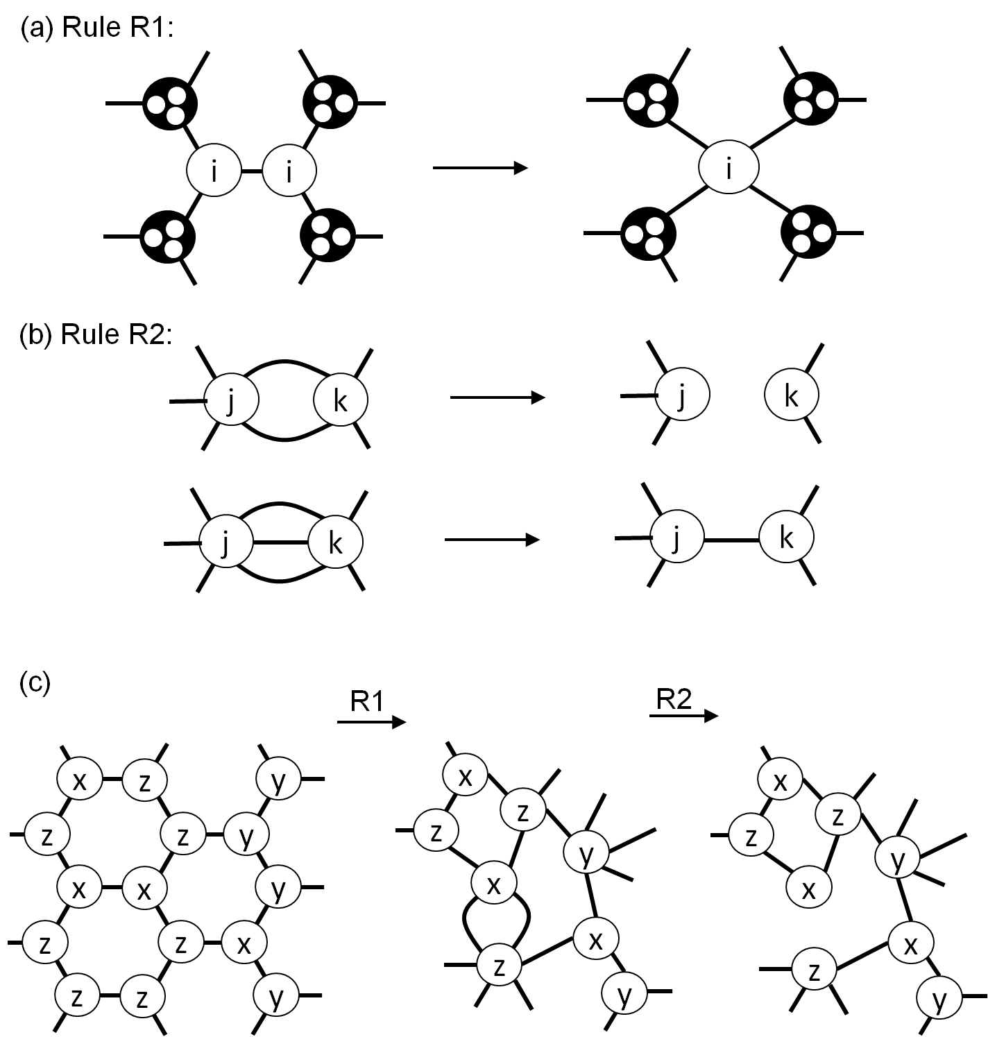
Figure 4: Graphical rules for transformation of the lattice ${\cal{L}}$ into the graph $G({\cal{A}})$, depending on the POVM outcomes ${\cal{A}}$. (a) Graph Rule 1: A single edge between neighboring sites with the same POVM outcome $i\in\{x,y,z\}$ is contracted. (b) Rule 2: Pairs of edges between the same vertices are deleted. (b) An example for the application of the rules 1 and 2 to a small honeycomb lattice. The alphabets ($j\neq k$) inside the circle indicate the POVM outcomes. (c) An example to illustrate the applications of the graph rules.

Rule 1: Merging of sites. Physically, this rule derives from the antiferromagnetic property of the AKLT state: neighboring spin-3/2 particles must not have the same $S_{a}=3/2$ (or -3/2) configuration AKLT ; AKLT2 ; AKLT3 . Hence, after the projection onto $S_{a}=\pm 3/2$ subspace by the POVM, the configurations for all sites inside a domain can only be $|3/2,-3/2,\dots\rangle$ or $|-3/2,3/2,\dots\rangle$, and intuitively, these form the basis of a single qubit. This encoding of a qubit can also be understood in terms of the stabilizer. Consider the case where two neighboring POVMs yield the same outcome, say $z$; see Fig. 5a. As a result of the projections $F_{u,z}$ and $F_{v,z}$ (with $u=\{1,2,3\}$ and $v=\{4,5,6\}$ each containing three virtual qubits), the operators $Z_{1}Z_{2}$, $Z_{2}Z_{3}$, and $Z_{4}Z_{5}$, $Z_{5}Z_{6}$ become stabilizer generators of the post-POVM state $|\Psi({\cal{A}})\rangle$. In addition, the stabilizer $-Z_{3}Z_{4}$ of the singlet state $|\phi\rangle_{34}$ commutes with the projection $F_{u,z}\otimes F_{v,z}$, and thus remains a stabilizer element for $|\Psi({\cal{A}})\rangle$. In summary, the stabilizer generators are $Z_{1}Z_{2},Z_{2}Z_{3},-Z_{3}Z_{4},Z_{4}Z_{5},Z_{5}Z_{6}$, giving rise to a single encoded qubit

$$\alpha|(000)_{u}(111)_{v}\rangle+\beta|(111)_{u}(000)_{v}\rangle,$$

which is supported by the two sites $u$ and $v$ jointly. We observe here the antiferromagnetic ordering AKLT ; AKLT2 ; AKLT3 among groups of three virtual qubits. To reduce the support of this logical qubit to an individual site of ${\cal{L}}$, a measurement in the basis $\{|(000)_{v}\rangle\pm|(111)_{v}\rangle\}$ is performed. The resulting state is $\alpha|(000)_{u}\rangle\pm\beta|(111)_{u}\rangle$, with the sign “$\pm$” known from the measurement outcome. This is the proper encoding for a domain consisting of a single site. Domains of more than two sites are thereby reduced to a single site in the same manner.

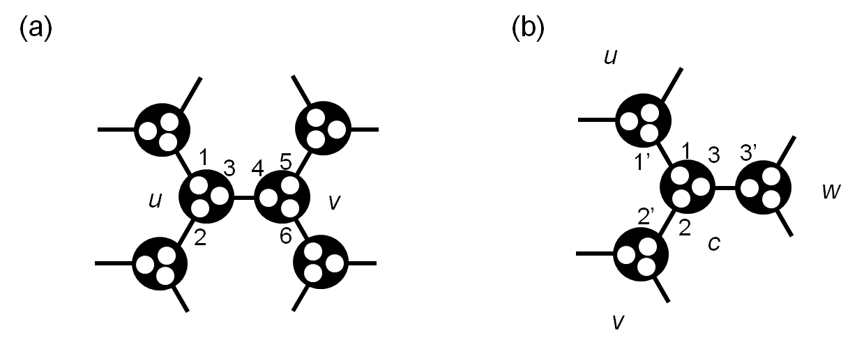
Figure 5: Illustrations of the encoding and the cluster graph stabilizer. (a) If two neighboring sites $u$ and $v$ share the same POVM outcome, e.g., $a_{u}=a_{v}=z$, then collectively these two sites form a logical qubit. More generally, if a set of connected sites share the same POVM outcome, then these sites effective encode a logical qubit. (b) An example of four sites $u$, $v$, $w$, and $c$ with POVM outcomes $a_{c}=z$, and $a_{u}=a_{v}=a_{w}=x$ is used to illustrate the stabilizer generator $K_{c}=\pm\bar{X}_{c}\bar{Z}_{u}\bar{Z}_{v}\bar{Z}_{w}$.

To see that the state $|\Psi({\cal{A}})\rangle$ is indeed equivalent under local unitary transformations to the encoded graph state $\overline{|G({\cal{A}})\rangle}$, we consider the example of four domains $c$, $u$, $v$, $w$, each consisting of a single site of ${\cal{L}}$, where the POVM outcome is $z$ on the central domain $c$ and $x$ on all lateral domains $u$, $v$ and $w$; see Fig. 5b. By similar arguments as above, the operator ${\cal O}\equiv-X_{1}X_{1^{\prime}}X_{2}X_{2^{\prime}}X_{3}X_{3^{\prime}}$ is in the stabilizer of $|\Psi({\cal{A}})\rangle$. Using the encoding in Table 2, i.e., with the encoded Pauli operators $\overline{X}_{c}=Z_{1}Z_{2}Z_{3}$, $\overline{Z}_{u}=\pm X_{1^{\prime}}$, $\overline{Z}_{v}=\pm X_{2^{\prime}}$, and $\overline{Z}_{w}=\pm X_{3^{\prime}}$, we find that ${\cal O}=\pm\overline{X}_{c}\overline{Z}_{u}\overline{Z}_{v}\overline{Z}_{w}$ which is (up to a possible sign of convention) one of the stabilizer generators defining the graph state. Intuitively, we see that each edge from an outer domain contributes to an encoded $\overline{Z}$ from that domain and the operator restricted at the center domain is clearly not an identity nor an encoded $\overline{Z}$ as its POVM outcome differs from the outer ones. This gives rise to a stabilizer generator local-unitarily equivalent to the one given in Eq. (29).

Rule 2: Mod 2 edge deletion. By the above construction, if two domains $u$, $v$ are connected by an edge of multiplicity $m$, the inferred graph state stabilizer generators will contain factors of $\overline{X}_{u}{\overline{Z}_{v}}^{m}$ or $\overline{X}_{v}{\overline{Z}_{u}}^{m}$. We observe that $Z^{2}=I$, from which Rule 2 follows.

Generalizing the above ideas, it is straightforward to rigorously prove that for any POVM outcomes for any ${\cal{A}}$, the state $|\Psi({\cal{A}})\rangle$ is local equivalent to an encoded graph state $\overline{|G({\cal{A}})\rangle}$; see below. We shall denote by $|G({\cal A})\rangle$ the graph state after reducing multiple sites in every domain to a single site, i.e., to the proper qubit encoding by domains, as the graph remains the same.

IV From the AKLT state to graph states: general proof

Let us recall the POVM to be performed on all sites can be rewritten as:

$$\begin{array}[]{rcl}F_{v,z}&=&\displaystyle{\sqrt{\frac{2}{3}}\frac{I_{12}+Z_{1}Z_{2}}{2}\frac{I_{23}+Z_{2}Z_{3}}{2}},\\ F_{v,x}&=&\displaystyle{\sqrt{\frac{2}{3}}\frac{I_{12}+X_{1}X_{2}}{2}\frac{I_{23}+X_{2}X_{3}}{2}},\\ F_{v,y}&=&\displaystyle{\sqrt{\frac{2}{3}}\frac{I_{12}+Y_{1}Y_{2}}{2}\frac{I_{23}+Y_{2}Y_{3}}{2}}.\end{array}$$ (32)

It turns out that, for any ${\cal{A}}$, the state $|\Psi({\cal{A}})\rangle$ is local equivalent to an encoded graph state $\overline{|G({\cal{A}})\rangle}$, with the graph $G({\cal{A}})$ constructed as follows. An edge $(v,w)\in E({\cal{L}})$ is called internal iff at the sites $v$ and $w$ the local POVM has resulted in the same outcome. The graph $G({\cal{A}})$ is obtained from the lattice graph ${\cal{L}}$ by (1) contracting all internal edges, and, in the resultant multi-graph, (2a) deleting all edges of even multiplicity and (2b) converting all edges of odd multiplicity into conventional edges of multiplicity 1. See Fig.2 for illustration.

In step (1) of the above procedure, several sites of ${\cal{L}}$ are merged into a single composite object ${\cal{C}}\in V(G({\cal{A}}))$. Each such ${\cal{C}}$ is both a vertex in the graph $G({\cal{A}})$ and a connected set of same-type sites of ${\cal{L}}$, i.e., a domain. Physically, in a domain of type $a$, we have antiferromagnetic order along the $\pm a$-direction, because two neighboring spins never have the same $S_{a}=3/2$ (or -3/2) in the AKLT state AKLT . The state of the domain contains only two configurations w.r.t. the quantization axis $a$: $|+3/2,-3/2,+3/2,\dots\rangle$ and $|-3/2,3/2,-3/2,\dots\rangle$. Thus, it is effectively one qubit.

The outlined construction leads to one of our main results:

Theorem 1

For any ${\cal{A}}$ that specifies all outcomes of POVMs on ${\cal L}$, quantum computation by local spin-3/2 measurements on the state $|\Psi({\cal{A}})\rangle$ can efficiently simulate quantum computation by local spin-1/2 measurement on the graph state $|G({\cal{A}})\rangle$.

Thus, the computational power of the AKLT state, as harnessed by the POVMs Eq. (32), hinges on the connectivity properties of $G({\cal{A}})$. If, for typical sets ${\cal{A}}$ of POVM outcomes, the graph state $|G({\cal{A}})\rangle$ is computationally universal then so is the AKLT state.

The proof proceeds in three steps. First we show that every domain ${\cal{C}}\in V(G({\cal{A}}))$ gives rise to one encoded qubit. Second, we show that $|\Psi({\cal{A}})\rangle$ is, up to local encoded unitaries, equivalent to the encoded graph state $\overline{|G({\cal{A}})\rangle}$. Third, we show that the encoding can be unraveled by local spin-3/2 measurements.

Step 1: Encoding. Consider a domain ${\cal{C}}\subset V({\cal{L}})$. That is, on all sites $v\in{\cal{C}}$ the same POVM outcome $a\in\{x,y,z\}$ was obtained. ${\cal{C}}$ contains $3|{\cal{C}}|$ qubits. The projections $F_{v,a}$ on all $v\in{\cal{C}}$ enforce $2|{\cal{C}}|$ stabilizer generators, c.f. Eq. (30). Furthermore, choose a tree ${\cal{T}}$ among the set of edges with both endpoints in the domain ${\cal{C}}$. Each edge $(u,v)\in{\cal{T}}$ contributes a stabilizer generator $-\sigma_{a}^{(u)}\sigma_{a}^{(v)}$ to the product of Bell states $\bigotimes_{e\in E({\cal{L}})}|\phi\rangle_{e}$. These stabilizers commute with the local POVMs (32) and therefore are also stabilizer generators for $|\Psi({\cal{A}})\rangle$. Since $|{\cal{T}}|=|{\cal{C}}|-1$, in total there are $3|{\cal{C}}|-1$ stabilizer generators with support only in ${\cal{C}}$, acting on $3|{\cal{C}}|$ qubits. They give rise to one encoded qubit.

While the stabilizer generators for our code follow from the construction, there is freedom in choosing the encoded Pauli operators. Table 2 shows one such choice of encoding.

POVM outcome	$z$	$x$	$y$
stabilizer generator	$\lambda_{i}\lambda_{i+1}Z_{i}Z_{i+1}$,	$\lambda_{i}\lambda_{i+1}X_{i}X_{i+1}$	$\lambda_{i}\lambda_{i+1}Y_{i}Y_{i+1}$
$\overline{X}$	$\bigotimes_{j=1}^{3|{\cal{C}}|}X_{j}$	$\bigotimes_{j=1}^{3|{\cal{C}}|}Z_{j}$	$\bigotimes_{j=1}^{3|{\cal{C}}|}Z_{j}$
$\overline{Z}$	$\lambda_{i}Z_{i}$	$\lambda_{i}X_{i}$	$\lambda_{i}Y_{i}$

Table 2: The dependence of stabilizers and encodings for the random graphs on the local POVM outcome. $|{\cal C}|$ denotes the total number of virtual qubits contained in a domain. In the first line, $i=1\,..\,3|{\cal{C}}|-1$, and in the third line $i=1\,..\,3|{\cal{C}}|$. The honeycomb lattice ${\cal{L}}$ is bicolorable or bipartite and all sites can be divided into either $A$ or $B$ sublattice, $V({\cal{L}})=A\cup B$. Then, one choice of the sign is $\lambda_{i}=1$ if the virtual qubit $i\in v\in A$ and $\lambda_{i}=-1$ if $i\in v^{\prime}\in B$.

Step 2: We show that $|\Psi({\cal{A}})\rangle$ is an encoded graph state. Consider a central vertex ${\cal{C}}_{c}\in V(G({\cal{A}}))$ and all its neighboring vertices ${\cal{C}}_{\mu}\in V(G({\cal{A}}))$. Denote the POVM outcome for all ${\cal{L}}$-sites $v\in{\cal{C}}_{c},{\cal{C}}_{\mu}$ by $a_{c}$ and $a_{\mu}$, respectively. Denote by $E_{\mu}$ the set of ${\cal{L}}$-edges that run between ${\cal{C}}_{c}$ and ${\cal{C}}_{\mu}$. Denote by $E_{c}$ the set of ${\cal{L}}$-edges internal to ${\cal{C}}_{c}$. Denote by $C_{c}$ the set of all qubits in ${\cal{C}}_{c}$, and by $C_{\mu}$ the set of all qubits in ${\cal{C}}_{\mu}$. (Recall that there are 3 qubit locations per ${\cal{L}}$-vertex $v\in{\cal{C}}_{c},{\cal{C}}_{\mu}$.) We first consider the stabilizer of the state $\bigotimes_{e\in E({\cal{L}})}|\phi\rangle_{e}$. For any $\mu$ and any edge $e\in E_{\mu}$, let $u(e)$ [$v(e)$] be the endpoint of $e$ in $C_{\mu}$ [$C_{c}$]. Then, for all $\mu$ and all $e\in E_{\mu}$ the Pauli operators $-\sigma_{a_{\mu}}^{({u(e)})}\sigma_{a_{\mu}}^{(v(e))}$ are in the stabilizer of $\bigotimes_{e\in E({\cal{L}})}|\phi\rangle_{e}$. Choose $b\in\{x,y,z\}$ such that $b\neq a_{c}$, and let, for any edge $e^{\prime}\in E_{c}$, $v_{1}(e^{\prime}),v_{2}(e^{\prime})\in C_{c}$ be qubit locations such that $e^{\prime}=(v_{1}(e^{\prime}),v_{2}(e^{\prime}))$. Then, for all $e^{\prime}\in E_{c}$, $-\sigma_{b}^{({v_{1}(e^{\prime})})}\sigma_{b}^{(v_{2}(e^{\prime}))}$ is in the stabilizer of $\bigotimes_{e\in E({\cal{L}})}|\phi\rangle_{e}$. Therefore, the product of all these operators,

$$O_{{\cal{C}}_{c}}=\pm\!\left(\bigotimes_{\mu}\bigotimes_{e\in E_{\mu}}\sigma_{a_{\mu}}^{(u(e))}\sigma_{a_{\mu}}^{(v(e))}\!\right)\!\!\left(\bigotimes_{e^{\prime}\in E_{c}}\sigma_{b}^{(v_{1}(e^{\prime}))}\sigma_{b}^{(v_{2}(e^{\prime}))}\!\!\right)$$ (33)

is also in the stabilizer of $\bigotimes_{e\in E({\cal{L}})}|\phi\rangle_{e}$.

We now show that $O_{{\cal{C}}_{c}}$ commutes with the local POVMs and is therefore also in the stabilizer of $|\Psi({\cal{A}})\rangle$. First, consider the central domain ${\cal{C}}_{c}$. The operator $O_{{\cal{C}}_{c}}$ acts non-trivially on every qubit in $C_{c}$, $O_{{\cal{C}}_{c}}|_{l}\neq I_{l}$ for all qubits $l\in C_{c}$. Furthermore, for all qubits $l\in C_{c}$, $O_{{\cal{C}}_{c}}\left|{}_{l}\right.\neq\sigma_{a_{c}}^{(l)}$. Namely, if $l\in C_{c}$ is connected by an edge $e\in E_{\mu}$ to ${\cal{C}}_{\mu}$, for some $\mu$, then $O_{{\cal{C}}_{c}}\left|{}_{l}\right.=\sigma_{a_{\mu}}^{(l)}\neq\sigma_{a_{c}}^{(l)}$ (for all $\mu$, $a_{\mu}\neq a_{c}$ by construction of $G({\cal{A}})$). Or, if $l\in C_{c}$ is the endpoint of an internal edge $e^{\prime}\in E_{c}$ then $O_{{\cal{C}}_{c}}\left|{}_{l}\right.=\sigma_{b}^{(l)}\neq\sigma_{a_{c}}^{(l)}$ ($a_{c}\neq b$ by above choice). Therefore, for any $i,j\in C_{c}$, $O_{{\cal{C}}_{c}}$ anticommutes with $\sigma_{a_{c}}^{(i)}$ and $\sigma_{a_{c}}^{(j)}$, and thus commutes with all $\sigma_{a_{c}}^{(i)}\sigma_{a_{c}}^{(j)}$. Thus, $O_{{\cal{C}}_{c}}$ commutes with the local POVMs Eq. (32) on all $v\in{\cal{C}}_{c}$.

Second, consider the neighboring domains ${\cal{C}}_{\mu}$. $O_{{\cal{C}}_{c}}\left|{}_{{\cal{C}}_{\mu}}\right.=\bigotimes_{j}\sigma_{a_{\mu}}^{(j)}$ by construction. $O_{{\cal{C}}_{0}}$ thus commutes with the local POVMs $F_{v,a_{\mu}}$ for all $v\in{\cal{C}}_{\mu}$ and for all $\mu$.

Therefore, $O_{{\cal{C}}_{c}}$ is in the stabilizer of $|\Psi({\cal{A}})\rangle$. Therefore, $O_{{\cal{C}}_{c}}$ is an encoded operator w.r.t. the code in Table 2, and we need to figure out which one. (1) Central vertex ${\cal{C}}_{c}$: $\left.O_{{\cal{C}}_{c}}|_{C_{c}}\right.$ is an encoded operator on $C_{c}$, $\left.O_{{\cal{C}}_{c}}|_{C_{c}}\right.\in\{\pm\overline{I},\pm\overline{X},\pm\overline{Y},\pm\overline{Z}\}$. Since $\left.O_{{\cal{C}}_{c}}|_{l}\right.\neq\sigma_{a_{c}}^{(l)}$ for any $l\in{\cal{C}}_{c}$, by Table 2, $\left.O_{{\cal{C}}_{c}}|_{C_{c}}\right.\neq\pm\overline{I},\pm\overline{Z}$. Thus, $\left.O_{{\cal{C}}_{c}}|_{C_{c}}\right.\in\{\pm\overline{X},\pm\overline{Y}\}$. (2) Neighboring vertices ${\cal{C}}_{\mu}$: By Table 2, $\sigma_{a_{\mu}}^{(l)}=\pm\overline{Z}$, for any $l\in C_{\mu}$. Thus, $\left.O_{{\cal{C}}_{c}}|_{C_{\mu}}\right.=\pm\overline{Z}^{|E_{\mu}|}$. Now observe that $Z^{2}=I$, and that, this justifies the above prescription in constructing the graph $G({\cal{A}})$. Using the adjacency matrix $A_{G({\cal{A}})}$, we have $|E_{\mu}|\mod 2=[A_{G({\cal{A}})}]_{c,\mu}$ and hence $\left.O_{{\cal{C}}_{c}}|_{C_{\mu}}\right.=\pm\overline{Z}^{[A_{G({\cal{A}})}]_{c,\mu}}$.

Thus, finally, for all ${\cal{C}}_{c}\in V(G({\cal{A}}))$,

$$O_{{\cal{C}}_{c}}\in\left\{\pm\overline{R}_{C_{c}}\bigotimes_{{\cal{C}}_{\mu}\in V(G({\cal{A}}))}\overline{Z}_{{\cal{C}}_{\mu}}^{[A_{G({\cal{A}})}]_{c,\mu}},\;\mbox{with }R=X,Y\right\}$$ (34)

This is, up to conjugation by one of the local encoded gates $\overline{I}_{{\cal{C}}_{c}},\overline{Z}_{{\cal{C}}_{c}},\exp\big{(}\pm i\pi/4\,\overline{Z}_{{\cal{C}}_{c}}\big{)}$, a stabilizer generator for the encoded graph state $\overline{|G({\cal{A}})\rangle}$. The code stabilizers in Table 2 and the stabilizer operators in Eq. (34) together define the state $|\Psi({\cal{A}})\rangle$ uniquely. $|\Psi({\cal{A}})\rangle$ is, up to the action of local encoded phase gates, an encoded graph state $|G({\cal{A}})\rangle$.

Step 3: Decoding of the code. We show that any domain ${\cal{C}}\in V(G({\cal{A}}))$ can be reduced to a single elementary site $w\in V({\cal{L}})$ by local measurement on all other sites $v\in{\cal{C}}$, $v\neq w$. For any such $v$, choose the measurement basis ${\cal{B}}_{a}$, $a\in\{x,y,z\}$, as follows

$$\begin{array}[]{rcl}{\cal{B}}_{x}&=&\left\{{(|+++\rangle\pm|---\rangle)}/{\sqrt{2}}\right\},\\ {\cal{B}}_{y}&=&\left\{{(|i,i,i\rangle\pm|-i,-i,-i\rangle)}/{\sqrt{2}}\right\},\\ {\cal{B}}_{z}&=&\left\{{(|000\rangle\pm|111\rangle)}/{\sqrt{2}}\right\}.\end{array}$$ (35)

These measurements map the symmetric subspace of the three-qubit states into itself and they can therefore be performed on the physical spin 3/2 systems.

Denote by ${\cal{S}}_{\cal{C}}$ and ${\cal{S}}_{{\cal{C}}\backslash v}$ the code stabilizer on the domain ${\cal{C}}\in V(G({\cal{A}}))$ and on the reduced domain ${\cal{C}}\backslash v$, respectively. Using standard stabilizer techniques Stabilizer it can be shown that the measurement Eq. (35) has the following effect on the encoding

$${\cal{S}}_{\cal{C}}\longrightarrow{\cal{S}}_{{\cal{C}}\backslash v},\;\overline{X}_{\cal{C}}\longrightarrow\pm\overline{X}_{{\cal{C}}\backslash v},\;\overline{Z}_{\cal{C}}\longrightarrow\overline{Z}_{{\cal{C}}\backslash v}.$$ (36)

The measurement (35) thus removes from ${\cal{C}}$ by one lattice site $v\in V({\cal{L}})$. We repeat the procedure until only one site, $w$, remains in ${\cal{C}}$, for each ${\cal{C}}\in V(G({\cal{A}}))$. In this way, ${\cal{S}}_{\cal{C}}\longrightarrow{\cal{S}}_{\{w\}}$, $\overline{X}_{\cal{C}}\longrightarrow\pm\overline{X}_{\{w\}}$, $\overline{Z}_{\cal{C}}\longrightarrow\overline{Z}_{\{w\}}$. Thus, $|\Psi(A)\rangle\longrightarrow\overline{U}_{\text{loc}}\overline{|G(A)\rangle}=:|G(A)\rangle$, where $U_{\text{loc}}$ is a local unitary, and the encoding in Table 2 has now shrunk to one site of ${\cal{L}}$ per encoded qubit, i.e. to three auxiliary qubits.

To complete the computation, the remaining encoded qubits are measured individually. Again, the measurement of an encoded qubit on a site $w\in{\cal{L}}$ is an operation on the symmetric subspace of three auxiliary qubits at $w$, and can thus be realized as a measurement on the equivalent physical spin 3/2. $\Box$

V Random graph states, percolation and 2D cluster states

Whether or not typical graph states $|G({\cal{A}})\rangle$ are universal resources hinges solely on the connectivity properties of $G({\cal{A}})$, and is thus a percolation problem Perc . We test whether, for typical graphs $G({\cal{A}})$,

1. The size of the largest domain scales at most logarithmically with the total number of sites $|V({\cal{L}})|$.

2. Let $S\subset{\cal{L}}$ be a rectangle of size $l\times 2l$ ($2l\times l$). Then, a path through $G|_{S}$ from the left to the right (top to bottom) exists with probability approaching 1 in the limit of large ${\cal{L}}$.

Note that Condition C1 is obeyed whenever the domains are microscopic, i.e., their size distribution is independent of $|{\cal{L}}|$ in the limit of large ${\cal{L}}$. Then, the size of the largest domain scales logarithmically in $|{\cal{L}}|$ Perc . Condition C2 ensures that the system is in the percolating phase.

Together with planarity, which holds for all graphs $G({\cal{A}})$ by construction, the conditions C1 and C2 are sufficient for the reduction of the random graph state to a standard universal cluster state. The proof given below extends a similar result already established for site percolation on a square lattice BPerc . The physical intuition comes from percolation theory. In the percolating (or supercritical) phase, the spanning cluster contains a subgraph which is topologically equivalent to a coarse-grained two-dimensional lattice structure. This subgraph can be carved out and subsequently cleaned off all imperfections by local Pauli measurements, leading to a perfect two-dimensional lattice.

V.1 Reduction of $|G({\cal{A}})\rangle$ to a 2D cluster state above the percolation threshold

We define the distance $\text{\em{dist}}_{\cal{L}}(v,w)$ between two vertices $v,w\in V({\cal{L}})$ as the minimum number of edges on a path between $u$ and $v$, and consider two further properties of graphs $G({\cal{A}})$:

1. $G({\cal{A}})$ can be embedded in ${\cal{L}}$ such that the maximum distance between the endpoints of an edge in $E(G)$ scales at most logarithmically in $|{\cal{L}}|$,

2. Let $S\subset{\cal{L}}$ be a rectangle of size $l\times 5l$ ($5l\times l$). Then, a path through $G|_{S}$ from the left to the right (top to bottom) exists with probability approaching 1 in the limit of large ${\cal{L}}$.

Lemma 1

$G({\cal{A}})$ is planar for all POVM outcomes ${\cal{A}}$. Property C1 implies property C1^′, and property C2 implies property C2 ^′.

Proof of Lemma 1. Planarity: $G({\cal{A}})$ is obtained from the honeycomb lattice ${\cal{L}}$, which is planar, by the graph rules R1 and R2. They only perform edge deletion and edge contraction, which preserve the planarity of ${\cal{L}}$. $G({\cal{A}}$ is thus planar for all ${\cal{A}}$.

Property C1^′: For any domain $d\subset V({\cal{L}})$, place the corresponding vertex $v(d)\in V(G({\cal{A}}))$ inside $d$ such that the distance $r(d):=\max_{w\in d}\text{dist}_{\cal{L}}(w,v)$ is minimized. Then, $r(d)\leq|d|/2$. Now, consider two vertices $v(d_{1}),v(d_{2})\in V(G)$ connected by an edge $e\in E(G)$. Then, the domains $d_{1}$, $d_{2}$ are connected by a single edge in $E({\cal{L}})$. Thus, for any pair $(v(d_{1}),v(d_{2}))$ of vertices in $G$ connected by an edge in $E(G)$, $\text{dist}_{\cal{L}}(v(d_{1}),v(d_{2}))\leq(|d_{1}|+|d_{2}|)/2+1$. By property C1, this length scales at most logarithmically in $|{\cal{L}}|$.

Property C2^′: See Fig. 6a.

Lemma 2

Consider a planar graph $G({\cal{A}}_{\cal{L}})$ embedded into the lattice ${\cal{L}}$ of size $\Lambda\times\Lambda$, satisfying the properties C1^′ and C2 ^′. Then, the graph state $|G({\cal{A}}_{\cal{L}})\rangle$ can be converted by local measurements to a two-dimensional cluster state of size $\Lambda^{\prime}\times\Lambda^{\prime}$, with $\Lambda^{\prime}\sim\Lambda/\log\Lambda$.

Both lemmata combined give the desired result:

Theorem 2

Consider an AKLT state on a honeycomb lattice ${\cal{L}}$ converted into a random graph state $|\overline{G({\cal{A}})}\rangle$ by the POVM (30). If for typical POVM outcomes ${\cal{A}}$ the corresponding graph $G({\cal{A}})$ satisfies the conditions C1 and C2, then the AKLT state is a universal resource for MBQC. Furthermore, the computation requires at most a poly-logarithmic overhead compared to cluster states.

Remark: The polylog bound to the overhead comes from bounding the average domain size by the maximum domain size, for technical reasons. The true overhead is expected to be constant.

That the conditions C1 and C2 are obeyed in the typical case remains to be demonstrated. We show this numerically, as reported in the next section.

Proof of Lemma 2 - main tool. We show that a graph state $|G\rangle$ satisfying the assumptions of Lemma 2 can be reduced to the cluster state on a two-dimensional square grid, by local Pauli measurement on a subset of its qubits. The 2D cluster state is already known to be universal Oneway . Specifically, we use the following rules Hein for the manipulation of graph states

$$\parbox{142.26378pt}{\includegraphics[width=142.26378pt]{GR1}},$$ (37a)

$$\parbox{142.26378pt}{\includegraphics[width=142.26378pt]{GR2}},$$ (37b)

$$\parbox{142.26378pt}{\includegraphics[width=142.26378pt]{GR3}}.$$ (37c)

Rule (37a): The effect of a $\sigma_{z}$-measurement at vertex $a$ on the interaction graph is to remove $a$ and all edges ending in $a$.
Rule (37b): The effect of a $\sigma_{y}$-measurement at vertex $a$ on the interaction graph is to invert all edges in the neighborhood $N(a)$ of $a$, and to remove $a$ and all edges adjacent to $a$.
Rule (37c): Consider three qubits on a line, where the middle qubit has exactly two neighbors. When the left and the middle qubit are measured in the $\sigma_{x}$-basis, the interaction graph changes as follows: The right vertex inherits the neighbors of the left vertex. The left and the middle vertex plus all edges adjacent to them are deleted.

Proof of Lemma 2 - Outline. We consider a graph $G$ with properties C1^′, C2^′. We impose a pattern of regions $A$, $B$, $C$, .. of rectangular shape and size $l\times 5l$ and $5l\times l$, for sufficiently large $l$, on the plane into which $G$ is embedded; See Fig. 6b. Due to the percolation property, $G$ has a net-shaped subgraph ${\cal{P}}$, shown in Fig. 7a. In the first step of the reduction all qubits in $V(G)\backslash V({\cal{P}})$ are measured individually in the $\sigma_{z}$-basis. The graph thereby created is close to the one displayed in Fig. 7b. However, it may have additional edges that cannot be removed by vertex deletion (37a) alone. Such edges are removed by a combination of the graph rules (37a) and (37b). Then, in two further steps, the graph state of Fig. 7b is converted to the 2D cluster state shown in Fig. 7d.

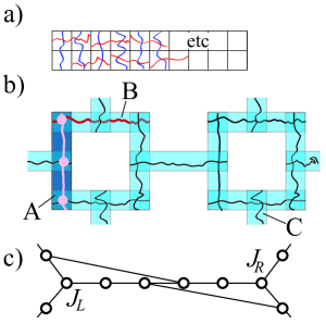
Figure 6: (a) Constructing a rectangle with a traversing path of aspect ratio 1:5, from such rectangles with aspect ratio 1:2, 2:1. (b) Overlapping rectangles of size $L\times 5L$, $5L\times L$. The union of their traversing paths yields the net ${\cal{P}}$. (c) Pair of non-separated junctions.

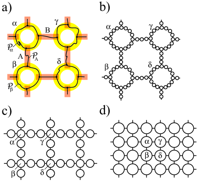
Figure 7: Transforming $|G({\cal{A}})\rangle$ into a 2D cluster state. (a) Macroscopic view: Regions $\alpha$, $\beta$, $A$ etc imposed on the graph $G({\cal{A}})$. (b) Graph with three-valent junctions. (c) Decorated 2D grid. (d) 2D grid for the cluster state.

Step 1. - Conversion of the graph $G$ to the graph of Fig. 7b by local operations. First we show that the net ${\cal{P}}$ of paths shown in Fig. 7a exists. Consider the overlapping rectangles $A$ and $B$ in Fig. 6b. By Property C2^′, $A$ has a path ${\cal{P}}_{A}$ running from top to bottom, and $B$ a path ${\cal{P}}_{B}$ crossing from left to right. Since $G$ is planar, ${\cal{P}}_{A}$ and ${\cal{P}}_{B}$ must intersect in at least one vertex. The net ${\cal{P}}$ is defined to be the union of all such traversing paths (one per rectangle), with all ends removed that do not affect connectedness. ${\cal{P}}$ is shown in Fig. 7a.

Now, $G$ is converted to $G|_{V({\cal{P}})}$, by deleting all vertices from $G$ which are not in $V({\cal{P}})$. Physically, the corresponding graph state $|G|_{V({\cal{P}})}\rangle$ is obtained by measuring the qubits at all vertices $v\in V(G)\backslash V({\cal{P}})$ in the eigenbasis of $\sigma_{z}$, c.f. Eq. (37a). After that, ideally, all junctions of paths in $G|_{V({\cal{P}})}$ should be T-shaped, as in the graph of Fig. 7b. However, in general they will not be. The quintessential (but not only) obstruction is

Note that no further edges can be removed by vertex deletion (corresponding to $\sigma_{z}$-measurements), without disconnecting the junction. Nonetheless, this obstruction is easily dealt with. The above ring junction is converted into a T-junction by a single measurement in the $\sigma_{y}$-basis,

(38)

However, we have to show that all possible obstructions to T-junctions can be removed.

We begin with the wires, running from one junction $J_{L}\in V(G|_{V({\cal{P}})})$ to another junction $J_{R}\in V(G|_{V({\cal{P}})})$. They also have obstructions, for example

The first goal is to remove all obstructions within each wire. We require that for a given wire, each belonging vertex, except $J_{L}$ and $J_{R}$, has a unique neighbor to the right and a unique neighbor to the left in the wire, to which it is connected by an edge. $J_{L}$ ($J_{R}$) only has a unique right but no left (a unique left but no right) neighbor in the wire. The vertices are allowed to have edges with vertices in other wires. Those will be removed later.

Note that the vertices in the wire are left-right ordered, by order of appearance in the corresponding percolation path. Now, the obstructions are removed from any given wire by the following procedure. Starting with $v=J_{L}$, take a vertex $v$ and identify its rightmost neighbor in the wire, $w$. Delete all vertices between $v$ and $w$. Now set $v:=w$, and repeat until $w=J_{R}$.

In this way, each vertex in the wire remains with a single right neighbor in the wire. Therefore, the number of edges within the wire equals the number of vertices minus 1. Therefore, each vertex in the wire also has a unique left neighbor.

At this stage we remain with the obstructions at junctions. First we show that we can treat the junctions individually, by choosing a sufficiently large length scale $l$ for the size $l\times 5l$- ($5l\times l$-) rectangles. Two neighboring junctions $J_{L}$, $J_{R}$ have a distance of at least $l$, c.f. Fig. 6b. They are separated if the configuration of edges shown in Fig. 6c does never occur. It doesn’t occur if $l>2|e|_{\text{max}}$, where $|e|_{\text{max}}$ is the maximum distance of an edge in $E(G({\cal{A}}))$. With C1^′ it thus suffices to choose

$$l\sim log\Lambda.$$ (39)

Now we discuss an individual junction $J$. By construction it joins three wires, $W_{L}$, $W_{C}$ and $W_{R}$ say. The obstructions are three sets of edges, $E_{LR}$, $E_{LC}$ and $E_{CR}$. They connect vertices in $W_{L}$ with vertices $W_{R}$, $W_{L}$ and $W_{C}$, and $W_{C}$ and $W_{R}$, respectively. By the choice Eq. (39) for $l$, the obstructions at different junctions are well separated from each other, and we can thus treat them individually.

First, we remove the obstructions $E_{LC}$ and $E_{CR}$, by the following procedure. We approach the junction at $J$ on the wire $W_{C}$. Denote by $v$ the first vertex in $W_{C}$ which is the endpoint of an edge $e\in E_{LC}\cup E_{CR}$. By rule (37a), delete all vertices in $W_{C}$ between $v$ and $J$, excluding $v$ and $J$. Then, there arise three cases. (1) $v$ is connected to a single vertex in $W_{L}\cup W_{R}$. (2) $v$ is connected to exactly two vertices $w_{1},w_{2}\in W_{L}\cup W_{R}$, and $w_{1}$, $w_{2}$ are neighbors in $W_{L}\cup W_{R}$. (3) $v$ is connected to exactly two vertices $w_{1},w_{2}\in W_{L}\cup W_{R}$, and $w_{1},w_{2}$ are not neighbors in $W_{L}\cup W_{R}$; or $v$ is connected to more than two vertices in $W_{L}\cup W_{R}$. Graphically, the cases look as follows (the obstructing edges $E_{LR}$ are not relevant in the present sub-step, and are not shown),

Case (1): The vertex $w$ is taken as the new junction center $J$, and the edge $(v,w)$ is included into $W_{C}$. Thereby, the obstructing edge sets $E_{LC}$ and $E_{CR}$ are removed. Case (2): The qubit on vertex $v$ is measured in the $\sigma_{y}$-basis; c.f. Eq. (38). Thereby, case (2) is reduced to case (1). Case (3): Denote the leftmost (rightmost) neighbor of $v$ in $W_{L}\cup W_{R}$ by $w_{L}$ ($w_{R}$). All vertices in $W_{L}\cup W_{R}$ between $w_{L}$ and $w_{R}$ are deleted, by $\sigma_{z}$-measurement on the corresponding qubits. Thereby, case (3) is reduced to case (1).

In the above procedure, the center $J$ of the junction may have shifted within $W_{L}\cup W_{R}$. Consequently, $W_{L}$ (to the left of $J$), $W_{R}$ (to the right of $J$) and $E_{LR}$ are modified. Due to the shift in the location of $J$, edges that were in $E_{LR}$ may have become obstructing edges internal to $W_{L}$ or to $W_{R}$. They are removed by re-running the previous procedure for removing obstructing edges internal to the wires. There are no new edges in $E_{LR}$.

By the above procedure, we have created a junction of three wires $W_{L}$, $W_{C}$ and $W_{R}$ which are free of all obstructions except for the set $E_{LR}$. These edges are now removed by approaching the new junction center $J$ from the wire $W_{L}$ and repeating the previous procedure.

Step 2 - Creating the decorated lattice graph of Fig. 7c. Consider a ring-shaped segment of the graph in Fig. 7b, with the four belonging T-junctions $\alpha$, $\beta$, $\gamma$ and $\delta$. The qubits on all vertices on the path between $\alpha$ and $\beta$ are measured in the $\sigma_{z}$-basis. The corresponding vertices are thereby removed, c.f. Eq. (37a). Regarding the path between $\alpha$ and $\delta$, we require that $\alpha$ and $\beta$ are not neighbors. This can always be arranged by starting with a sufficiently large scale $l$ for the $l\times 5l$-rectangles. If the the number of vertices that lie on the path between $\alpha$ and $\delta$ is even (but $>0$), then the qubit on the vertex next to $\alpha$ is measured in the $\sigma_{y}$-basis. In this way, the number of vertices between $\alpha$ and $\delta$ becomes odd, c.f. Eq. (37b). Now, $\alpha$ and the vertex next to it are measured in the $\sigma_{x}$-basis. By Eq. (37c), $\alpha$ moves two vertices closer to $\delta$ This procedure is repeated until $\alpha$ and $\beta$ are merged into a single vertex $\alpha^{\prime}$. Then, in an analogous manner, $\alpha^{\prime}$ is merged with $\gamma$, and with $\beta$. Thereby, the ring of four T-junctions is converted into a single vertex of degree 4.

Step 3 - Creating the square lattice graph of Fig. 7d. By the same method as in Step 2, the line segments between the vertices of degree 4 are contracted. This creates a two-dimensional cluster state on a square lattice, which is known to be a universal resource for measurement-based quantum computation Oneway . Since only local measurements were used in the reduction, the original graph state $|G\rangle$ is universal as well.

Overhead: The bottleneck of the construction is to guarantee that all junctions can be treated individually, which requires $L\sim\log\Lambda$, c.f. Eq. (39). As displayed in Fig. 6b, a qubit in the created planar cluster state claims an area of size $8l\times 8l$ on the original honeycomb lattice ${\cal{L}}$, and thus $\Lambda^{\prime}\sim\Lambda/\log\Lambda$, as claimed. $\Box$

Our proof thus generalizes the results in Ref. BPerc to random graphs. This extends the set of cluster-type universal states to more general 2D random graph states and beyond regular lattices Universal .

VI Monte Carlo simulations

We give the recipe for performing Monte Carlo simulations and present some results.
(1) First, we randomly assign every site on the honeycomb lattice to be either $x$, $y$ or $z$-type with equal probability.
(2) Second, we use the Metropolis method to sample typical configurations. For each site we attempt to flip the type to one of the other two with equal probability. Accept the flip with a probability $p_{\rm accept}=\min\left\{1,2^{|V^{\prime}|-|{\cal E}^{\prime}|-|V|+|{\cal E}|}\right\}$, where $|V|$ and $|{\cal E}|$ denote the number of domains and inter domain edges (before the modulo-2 operation on inter-domain edges; see Fig. 2 of main text), respectively before the flip, and similarly $|V^{\prime}|$ and $|{\cal E}^{\prime}|$ for the flipped configuration. The counting of $|V|$ and $|{\cal E}|$, etc. is done via a generalized Hoshen-Kopelman algorithm HoshenKopelman . For the proof of the probability ratio, see Sec. VI.1.

(3) After many flipping events, we measure the properties regarding the graph structure for the domains and study their percolation properties upon deleting edges. For the percolation, we cut open the lattice and investigate the percolation threshold for the typical random graphs from the Metropolis sampling.

VI.1 Evaluation of probability ratio

In this section, we shall explain the transition probability ratio: $p_{\rm accept}=\min\left\{1,2^{|V^{\prime}|-|{\cal E}^{\prime}|-|V|+|{\cal E}|}\right\}$, which arises from the probability for POVM outcomes $\{a_{v}\}$ being $p(\{a_{v}\}\sim 2^{|V|-|{\cal E}|}$, where $|V|$ and $|{\cal E}|$ denote the number of domains and inter-domain edges (before the modulo-2 operation). The proof is very similar to that in 1D. For convenience, we shall use spin-3/2 representation of the AKLT state. The local mapping from three virtual qubits to one spin-3/2 is

$$\hat{P}_{v}=|1\rangle\langle 000|+|2\rangle\langle 111|+|3\rangle\langle W|+|4\rangle\langle\overline{W}|,$$ (40)

where we have simplified the notation for the spin-3/2 basis states: $|1\rangle\equiv|3/2,3/2\rangle$, $|2\rangle\equiv|3/2,-3/2\rangle$, $|3\rangle\equiv|3/2,1/2\rangle$ and $|4\rangle\equiv|3/2,-1/2\rangle$. Moreover, $|000\rangle$, $|111\rangle$, $|W\rangle$ and $|\overline{W}\rangle$ constitute the basis states for the symmetric subspace of three spin-1/2 particles. The AKLT state can then be expressed as

$$|\psi\rangle_{\rm AKLT}=\mathop{\bigotimes}_{v}\hat{P}_{v}\prod_{e=(u,v)\in E}|\phi\rangle_{e},$$ (41)

where $|\phi\rangle_{e}$ is the singlet state $(|01\rangle-|10\rangle)_{u_{i},v_{j}}$ for the edge $e=(u,v)$ and $i,j$ specify the virtual qubit in the respective vertex.

The POVM that reduces the spin-3/2 AKLT to a spin-1/2 graph state consists of elements $E_{\mu}=F_{\mu}^{\dagger}F_{\mu}$ such that $\openone=E_{x}+E_{y}+E_{z}$, with

$$\hat{F}_{z}=\hat{F}_{z}^{\dagger}\equiv\sqrt{\frac{2}{3}}(|1\rangle\langle 1|+|2\rangle\langle 2|)=\frac{1}{\sqrt{6}}\big{(}S_{z}^{2}-\frac{1}{4}\big{)},$$ (42)

$$\hat{F}_{x}=\hat{F}_{x}^{\dagger}\equiv\sqrt{\frac{2}{3}}(|a\rangle\langle a|+|b\rangle\langle b|)=\frac{1}{\sqrt{6}}\big{(}S_{x}^{2}-\frac{1}{4}\big{)},$$ (43)

$$\hat{F}_{y}=\hat{F}_{y}^{\dagger}\equiv\sqrt{\frac{2}{3}}(|\alpha\rangle\langle\alpha|+|\beta\rangle\langle\beta|)=\frac{1}{\sqrt{6}}\big{(}S_{y}^{2}-\frac{1}{4}\big{)},$$ (44)

where we have also expressed $\hat{F}$’s in terms of the corresponding spin operators. The other four states other than $|1\rangle$ and $|2\rangle$ are

$$|a\rangle\equiv|S_{x}=3/2\rangle=\frac{1}{\sqrt{8}}(|1\rangle+|2\rangle+\sqrt{3}|3\rangle+\sqrt{3}|4\rangle)$$ (45)

$$|b\rangle\equiv|S_{x}=\!-\!3/2\rangle=\frac{1}{\sqrt{8}}(|1\rangle-|2\rangle-\sqrt{3}|3\rangle+\sqrt{3}|4\rangle)$$ (46)

$$|\alpha\rangle\equiv|S_{y}=3/2\rangle=\frac{1}{\sqrt{8}}(|1\rangle-i|2\rangle+i\sqrt{3}|3\rangle-\sqrt{3}|4\rangle)$$ (47)

$$|\beta\rangle\equiv|S_{y}=\!-\!3/2\rangle=\frac{1}{\sqrt{8}}(|1\rangle+i|2\rangle-i\sqrt{3}|3\rangle-\sqrt{3}|4\rangle).$$ (48)

They correspond to the four virtual three-spin-1/2 states (in addition to $|000\rangle$ and $|111\rangle$) $|+++\rangle,|---\rangle,|\,\,i\,\,i\,\,i\rangle$ and $|\!-\!i,\!-\!i,\!-\!i\rangle$.

While the outcome of POVM constructed above at each site is random (either $x$, $y$ or $z$), outcomes at different sites may be correlated. For a particular set of outcomes $\{a_{v}\}$ at sites $\{v\}$, the resultant state is transformed to the following un-normalized state

$$|\psi^{\prime}\rangle=\mathop{\bigotimes}_{v}\hat{F}_{v,a_{v}}|\psi\rangle_{\rm AKLT},$$ (49)

with the probability being

$$p_{\{a_{v}\}}=\langle\psi^{\prime}|\psi^{\prime}\rangle/\langle\psi|\psi\rangle_{\rm AKLT}.$$ (50)

As $\hat{F}$’s are proportional to projectors, in evaluating the relative probability for two sets of outcome ${\{a_{v}\}}$ and ${\{b_{v}\}}$, one has

$$p_{\{a_{v}\}}/p_{\{b_{v}\}}=\langle\psi|\mathop{\bigotimes}_{v}\hat{F}_{v,a_{v}}|\psi\rangle_{\rm AKLT}\big{/}\langle\psi|\mathop{\bigotimes}_{v}\hat{F}_{v,b_{v}}|\psi\rangle_{\rm AKLT},$$ (51)

where we have used $\hat{F}_{v,a}^{2}\sim\hat{F}_{v,a}$. In order to evaluate the probability ratio for two different sets of configuration, we first note that

$$\hat{F}_{x}\hat{P}\sim|a\rangle\langle+++|+|b\rangle\langle---|$$ (52)

$$\hat{F}_{y}\hat{P}\sim|\alpha\rangle\langle i\,i\,i|+|\beta\rangle\langle-i-i-i|$$ (53)

$$\hat{F}_{z}\hat{P}\sim|1\rangle\langle 000|+|2\rangle\langle 111|.$$ (54)

The spin-3/2 state is transformed by $\bigotimes_{v}F_{v,a_{v}}$ to an effective spin-1/2 one, with the two levels being labeled by $(a,b)$, $(\alpha,\beta)$, or $(1,2)$, depending on which $\hat{F}$ is applied. The probability $p_{\{a_{v}\}}$ is essentially obtained by summing the square norm of the coefficients for all possible spin-1/2 constituent basis states (e.g. $|a\,b+0\,i\dots\rangle$ is a basis state). First we need to know how many different constituent states, and the number is related to how many effective spin-1/2 particles we have. For the sites that have same type of outcome ($x$, $y$ or $z$), they basically form a superposition of two Neél-like states, thereby corresponding to an effective spin-1/2 particle. This can be seen from the valence-bond picture that, e.g., for $r,s\in\{0,1\}$ we have $\langle rs|01-10\rangle=\pm\delta_{r,1-s}$. On the other hand, for $r\in\{0,1\}$ and $s\in\{+,-\}$, $\langle rs|01-10\rangle=\pm 1/\sqrt{2}$, which is $1/\sqrt{2}$ smaller than if $r$ and $s$ are the indices in the same basis. This means that all four combinations $\{0+,0-,1+,1-\}$ occur with equal amplitude up to a phase. (Similar consideration applies to other combinations of bases.) Therefore, the number of effective spin-1/2 particles is given by the number of domains, which we label by $|V|$. Notice that we have assumed that any domain does not contain a cycle with odd number of original sites, as no Neél state can be supported on such a cycle (or loop). Configurations with domains that contain a cycle with odd number need to be removed. Fortunately, as the honeycomb lattice is bi-partite, therefore any cycle must contain even number of sites and we do not to deal with the above complication.

What about the amplitude for each spin configuration? Furthermore, what is the probability of obtaining a particular set of outcome $\{a_{v}\}$? We have seen that for each inter-domain edge there is a contribution to a factor of $1/\sqrt{2}$ in the amplitude (as the end sites of the edge correspond to different types). Thus, the amplitude for each spin configuration gives an overall value (omitting the phase factor) of $2^{-|{\cal E}|/2}$ and hence a probability weight $2^{-|{\cal E}|}$, where $|{\cal E}|$ counts the number of inter-domain edges. As there are $2^{|V|}$ such configurations, we have the norm square of the resultant spin-1/2 state being proportional to $p\sim 2^{|V|-|{\cal E}|}$. For convenience, we have assume the lattice is periodic, but the argument holds for open boundary condition in which the spin-3/2’s at the boundary are either (1) suitably linked by to one another, preserving the trivalence or (2) terminated by spin-1/2’s. In the Appendices, we have provided an alternative derivation of the probability expression.

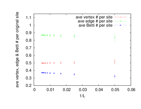
Figure 8: (color online) Average vertex (or domain) number, average edge number, and average Betti number in the typical random graphs original lattice site vs. $L$. The total number of sites is $N=L^{2}$. This shows the number of domains, the number of interdomain Ising interaction, and the number of independent loops in the resultant graph all scale with the system size of the original honeycomb lattice.

VI.2 Discussions of simulation results

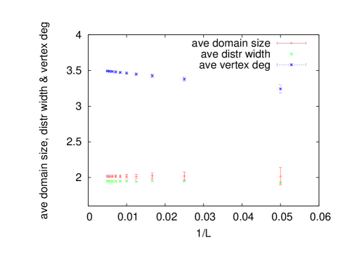
Figure 9: (color online) Average domain size (i.e., number of original sites in a domain), average width of domain size distribution, and average degree of a vertex in the typical random graphs vs. $L$, where $L^{2}$ is the total number of sites in the honeycomb lattice. For better discernibility of the two lower sets of data, we suppress the errorbars for one of them. This set of data was first shown in Ref. WeiAffleckRaussendorf11 , and we have reproduced it here for the sake of completeness.

We have analyzed lattices of size up to $200\times 200$ sites. As shown in Fig. 8, the size dependence of average vertex number, average edge number, and average Betti number $B$ Betti of the random graphs formed by domains relative to the original lattice size behaves as follows: $|\bar{V}|=0.495(2)L^{2}$, $|\bar{E}|=0.872(4)L^{2}$, and $\bar{B}=0.377(2)L^{2}$, where $L$ is related to the total number of sites in the original honeycomb lattice $N=L\times L$. This shows that the typical random graph of the graph state retains macroscopic number of vertices, edges, and cycles, giving strong evidence that the state is a universal resource. Figure 9 shows the average degree of a vertex vs. inverse system length $1/L$ for the random graphs, as well as the average numbers of the original sites contained in a typical domain. The average vertex degree extrapolates to $\bar{d}\approx 3.52(1)$ for the infinite system. This compares to $4$ for the square lattice and $3$ for the honeycomb lattice.

In order to show the stability of the random graph, we investigate how robust it is upon, e.g., deleting vertices (or edges) probabilistically, i.e., performing the site (or bond) percolation simulations. As shown in Fig. 10a, it requires the probability of deleting vertices to be as high $p_{\rm delete}=0.33(1)$ (i.e., percolation threshold $p_{\rm c}=0.67(1)$) in order to destroy the spanning property of the graph. This lies between the site percolation thresholds $\approx 0.592$ of the square lattice and $\approx 0.697$ of the honeycomb lattice. For bond percolation as shown in Fig. 10b, it takes a probability of $p_{\rm delete}=0.43(1)$ (i.e., percolation threshold $p_{\rm c}=0.57(1)$) to destroy the spanning property of the graph. Again, this threshold lies between that of the square lattice ($1/2$) and that of the honeycomb lattice ($\approx 0.652$). This shows that there exists many paths (proportional to the system’s linear size) on the random graphs that can be used to simulate one-qubit unitary gates on as many logical qubits and entangling operations among them. We remark that percolation argument was previously employed by Kieling, Rudolph, and Eisert in establishing the universality of using nondeterministic gates to construct a universal cluster state KielingRudolphEisert .

(a)

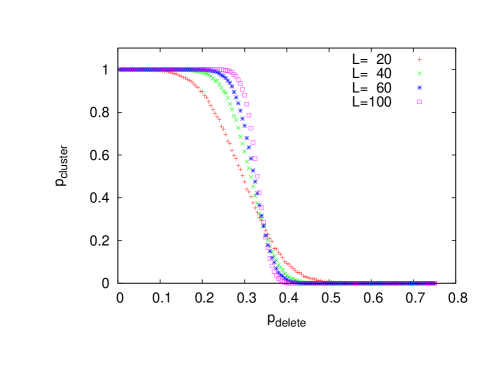
(b)

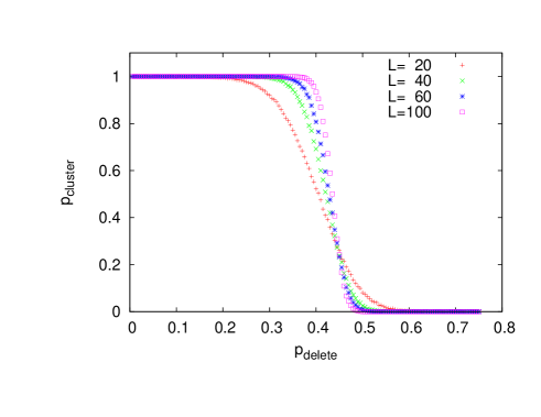
Figure 10: (color online) Percolation study of the graph formed by the domains: probability of a spanning cluster $p_{\rm cluster}$ vs. the probability to delete a vertex (top panel a) or an edge (bottom panel b) $p_{\rm delete}$. The threshold for destroying the spanning cluster is around $p_{\rm delete}\approx 0.33$ in deleting vertices and $p_{\rm delete}\approx 0.43$ in deleting edges. This shows that the graph without deleting any vertex or edge is deep in the percolated (i.e., connected) phase. We note that the result of site percolation is reproduced from Ref. WeiAffleckRaussendorf11 , and the additional bond percolation result presented here is consistent with the picture that the typical random graphs lie somewhat between the honeycomb and the square lattice.

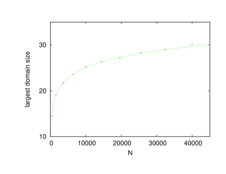
Figure 11: (color online) The largest domain size in the typical graphs vs. $L$, with $N=L^{2}$ being the total number of sites. The fitted curve to the largest domain size is $3.337\ln(N)-5.566$. The result is reproduced from Ref. WeiAffleckRaussendorf11 .

Let us also examine the two conditions listed in Sec. V.1.
Condition C1. For all POVM outcomes sampled from, the size of the largest domain was never macroscopic and it can at best be logarithmic in the original system size; see Fig. 11. The average number of sites $v\in V({\cal{L}})$ contained in a typical domain, when extrapolated to the infinite system, is $2.02(1)$; see Fig. 9. Our numerical simulations thus show that condition C1 holds.

Condition C2. For all of the POVM outcomes sampled, a horizontal and a vertical traversing path through the resulting graphs $G({\cal{A}})$ always existed (without deleting any vertex or edge). Our numerical simulations show that our random graph are deep in the supercritical phase and thus condition C2 holds.

In addition, a necessary condition for the computational universality of the graph states $|G({\cal{A}})\rangle$ is that typical graphs $G({\cal{A}})$ are not close to trees, because MBQC on tree-like graphs can be efficiently classically simulated Shi . For typical graphs $G({\cal{A}})$, we find that the Betti number (which is zero for trees) is proportional to the size of the initial honeycomb graph, with $\bar{B}=0.377(2)N$.

Robustness. We now quantify how deep typical graphs $G({\cal{A}})$ are in the connected phase of the percolation transition. A first measure is the average vertex degree. A heuristic argument based on a branching process suggests that a graph has a macroscopic connected component whenever the average vertex degree is $\bar{d}>2$. This criterion is exact for random graphs of uniform degree Perc . It also holds surprisingly well for lattice graphs footnote , which are the least random. In our case, the typical graphs $G({\cal{A}})$ have an average degree of 3.52, suggesting that the system is deep in the connected phase, which is confirmed by the percolation simulations. The existence of finite percolation thresholds (for both site and bond percolation) discussed earlier further supports the robustness of the connectedness.

VII Concluding remarks

We investigated the measurement-based quantum computation on the AKLT states. First we provided an alternative proof that the 1D spin-1 AKLT state can be used to simulate arbitrary one-qubit unitary gates. We extended the same formalism and demonstrated that the spin-3/2 AKLT state on a two-dimensional honeycomb lattice is a universal resource for measurement-based quantum computation by showing that a 2D cluster state can be distilled by local operations. Along the way, we connected the quantum computational universality of 2D random graph states to their percolation property and showed those 2D graph states whose graphs are in the supercritical phase are indeed universal resources for MBQC.

The key ingredient that has enabled our proof of computational universality for the (spin-3/2) 2D AKLT state on the honeycomb lattice is the generalized measurement in Eq. (30). How about the case of (spin-2) 2D AKLT state on the square lattice or any other lattices beyond trivalence is universal for MQBC. The AKLT spin-2 particle can be regarded as four virtual qubits in the symmetric subspace. Hence a naive extension of the POVM prompts us to consider the follow operators:

$${F}_{z} = (|0^{\otimes 4}\rangle\langle 0^{\otimes 4}|+|1^{\otimes 4}\rangle\langle 1^{\otimes 4}|)$$ (55a)

$${F}_{x} = (|+^{\otimes 4}\rangle\langle+^{\otimes 4}|+|-^{\otimes 4}\rangle\langle-^{\otimes 4}|)$$ (55b)

$${F}_{y} = (|i^{\otimes 4}\rangle\langle i^{\otimes 4}|+|-\!i^{\otimes 4}\rangle\langle-\!i^{\otimes 4}|).$$ (55c)

Unfortunately, $\sum_{\alpha}F^{\dagger}F^{\dagger}$ is not proportional to the projection onto the symmetric subspace. However, we can consider additionally the four states $|\gamma_{k}\rangle$ ($k=1,..,4$) such that their Bloch vectors point in the four diagonal directions of a cube, i.e., $(1,1,1)/\sqrt{3}$, $(-1,1,1)/\sqrt{3}$, $(-1,-1,1)/\sqrt{3}$, and $(1,-1,1)/\sqrt{3}$, respectively. Together with their corresponding conjugate states $|\bar{\gamma}_{k}\rangle$ having opposite vectors, we have four other sets of projections:

$$G_{k}\equiv|\gamma_{k}^{\otimes 4}\rangle\langle\gamma_{k}^{\otimes 4}|+|\bar{\gamma}_{k}^{\otimes 4}\rangle\langle\bar{\gamma}_{k}^{\otimes 4}|.$$ (56)

It can be checked that

$$\frac{8}{24}\sum_{\alpha=x,y,z}F^{\dagger}_{\alpha}F_{\alpha}+\frac{9}{24}\sum_{k=1}^{4}G^{\dagger}_{k}G_{k}=P_{S},$$ (57)

where $P_{S}$ is the projection operator onto the symmetric subspace of four qubits LiEtAl . However, such a generalized measurement would yield four additional pairs of states $\{\gamma_{k},\bar{\gamma}_{k}\}$ which are not mutually unbiased to one another nor to the eigenstates of the three Pauli operators. Due to this complication, whether the 2D AKLT state on the square lattice is universal for MQBC remains open.

Acknowledgment. This work was supported by NSERC, CIFAR, the Sloan Foundation, and the C.N. Yang Institute for Theoretical Physics.

Appendix A Calculation of probability of a particular POVM outcome using Arovas-Auerbach-Haldane techniques

In this appendix we provide an alternative formulation to the calculation of POVM outcome probability. This formalism has the potential of being applicable to a more general case. We give only the important ingredients here.

Arovas, Auerbach and Haldane (AAH) Arovas show how to represent arbitrary AKLT states as Boltzmann weights for nearest neighbour statistical mechanical models in the same spatial dimension as the quantum problem and how to represent calculations of equal time ground state expectation values classically. We are interested in two cases: the $S=1$ one-dimensional case and the $S=3/2$ honeycomb lattice case.

In both cases the operators of interest are proportional to projection operators onto maximal $|S^{z}|$:

$$F_{\nu} \equiv (S_{\nu})^{2}/\sqrt{2},\ \ (S=1)$$ (58)

$$\equiv [(S_{\nu})^{2}-1/4]/\sqrt{6},\ \ (S=3/2),$$ (59)

where $\nu=x,y\,{\rm or}\,z$ and, for convenience, we have rescaled the prefactor in the definition of $F$’s. For general spin S the operators $S^{a}$ are represented first in terms of Schwinger bosons, $a$, $a^{\dagger}$, $b$, $b^{\dagger}$, then in terms of co-ordinates and derivatives $u$, $v$, $\partial_{u}$, $\partial_{v}$ acting on homogeneous polynomials of $O(2S)$. The operator $(S^{z})^{2}$ is:

$$(S^{z})^{2}=(1/4)(a^{\dagger}a-b^{\dagger}b)^{2}=(1/4)(\partial_{u}u-\partial_{v}v)^{2}$$

$$=(1/4)(\partial_{u}^{2}u^{2}+\partial_{v}v^{2}-2\partial_{u}\partial_{v}uv-\partial_{u}u-\partial_{v}v).$$ (60)

We now use the prescription of Arovas, Auerbach and Haldane:

$$\langle\psi^{\prime}|\partial_{u}^{k}\partial_{v}^{l}u^{k+j}v^{l-j}|\psi\rangle$$

$$=\left[\prod_{m=2}^{k+l+1}(2S+m)\right]\langle\psi^{\prime}|u^{*k}v^{*l}u^{k+j}v^{l-j}|\psi\rangle$$ (61)

for any states $|\psi^{\prime}\rangle$ and $|\psi\rangle$ in the spin $S$ Hilbert space.

To prove Eq. (61), note that a complete set of states for the spin $S$ Hilbert space is given by $u^{S+m}v^{S-m}$ which are eigenstates of $S^{z}$ with eigenvalue $m=-S,-S+1,\ldots S$. To prove Eq. (61) for $j=0$, we wish to prove:

$$\int d^{2}\Omega u^{*S+m}v^{*S-m}\partial_{u}^{k}\partial_{v}^{l}u^{k+S+m}v^{l+S-m}$$ (62)

$$= \left[\prod_{r=2}^{k+l+1}(2S+r)\right]\int d^{2}\Omega|u|^{2(S+m+k)}|v|^{2(S-m+l)}.$$

To prove this, we use the identity:

$$I_{p,q} \equiv \int d^{2}\Omega|u|^{2p}|v|^{2q}$$ (63)

$$= 2\pi(1/2)^{p+q}\int_{-1}^{1}dx(1+x)^{p}(1-x)^{q}$$

$$= 4\pi p!q!/(p+q+1)!$$

Thus the left hand side of Eq. (62) may be written:

$$LHS = {(S+m+k)!\over(S+m)!}{(S-m+l)!\over(S-m)!}I_{S+m,S-m}$$ (64)

$$= 4\pi{(S+m+k)!(S-m+l)!\over(2S+1)!}$$

$$= \left[\prod_{r=2}^{k+l+1}(2S+r)\right]I_{S+m+k,S-m+l}$$

which is the RHS. Furthermore, all off-diagonal matrix elements vanish for both the left and right hand side of the identity in Eq. (61) for $j=0$. That follows since $\psi^{*}_{m}\psi_{m^{\prime}}\propto e^{i(m^{\prime}-m)\phi}$ where $\phi$ is the azimuthal angle for the integration over the sphere. Neither inserting the operator on the left hand side of Eq. (61) nor multiplying by the function on the right hand side changes this azimuthal angle dependence, implying vanishing integrals. While it may appear that this proof only holds for $j=0$ in Eq. (61) it actually covers the case of general $j$. In general, Eq. (62) gives the $\langle\psi_{m}|\ldots|\psi_{m-j}\rangle$ matrix elements of the identity in Eq. (61), which are the only non-zero matrix elements. Furthermore the identity immediately generalizes to an arbitrary product on different lattice sites:

$$\langle\psi^{\prime}|\prod_{i}\partial_{u_{i}}^{k_{i}}\partial_{v_{i}}^{l_{i}}u_{i}^{k_{i}+j_{i}}v_{i}^{l_{i}-j_{i}}|\psi\rangle=\left[\prod_{i}\prod_{m=2}^{k_{i}+l_{i}+1}(2S+m)\right]$$

$$\times\langle\psi^{\prime}|\prod_{i}|u_{i}^{*k_{i}}v_{i}^{*l_{i}}u_{i}^{k_{i}+j_{i}}v_{i}^{l_{i}-j_{i}}|\psi\rangle$$ (65)

since we may simply extend the above argument to the basis states $\prod_{i}u_{i}^{S+m_{i}}v_{i}^{S-m_{i}}$ for which the matrix elements simply factorize. Since we have proved this identity for a complete set of states it follows for any states $|\psi\rangle$, $|\psi^{\prime}\rangle$ in the spin-$S$ Hilbert space, including the AKLT states.

Eq. (61) gives:

$$(S^{z})^{2} = (1/4)(2S+2)(2S+3)[|u|^{4}+|v|^{4}-2|u|^{2}|v|^{2}]$$ (66)

$$-(1/4)(2S+2)(|u|^{2}+|v|^{2})$$

$$= (1/4)(2S+2)(2S+3)[|u|^{2}-|v|^{2}]^{2}$$

$$-(1/2)(S+1)(|u|^{2}+|v|^{2}).$$

Using $u=\cos(\theta/2)e^{i\phi/2}$, $v=\sin(\theta/2)e^{-i\phi/2}$, where $\theta$ and $\phi$ are the polar and azimuthal angle on the unit sphere, this becomes:

$$(S^{z})^{2}=(1/4)(2S+2)(2S+3)(\Omega^{z})^{2}-(1/2)(S+1)$$ (67)

where $\Omega_{z}=\cos\theta$ is the projection of the unit vector onto the $z$-axis. A simple explicit calculation similar to this one shows that, for $\nu=x$, $y$ or $z$:

$$(S_{\nu})^{2}=(1/4)(2S+2)(2S+3)(\Omega^{\nu})^{2}-(1/2)(S+1)$$ (68)

as expected by SO(3) symmetry. This is a somewhat surprising formula in that the classical quantities are not positive semi-definite. Note that this formula is valid independent of the wave-function. The projection operators thus become:

$$F_{\nu} = [5(\Omega^{\nu})^{2}-1]/\sqrt{2},\ \ (S=1)$$ (69)

$$= \sqrt{3/8}\,[5(\Omega^{\nu})^{2}-1],\ \ (S=3/2).$$ (70)

Remarkably the projection operators are the same for $S=1$ and 3/2 up to an unimportant normalization factor.

The AKLT state can be written, in Schwinger boson notation as:

$$|\psi\rangle_{\rm AKLT}=\prod_{\langle i,j\rangle}(a^{\dagger}_{i}b^{\dagger}_{j}-a^{\dagger}_{j}b^{\dagger}_{i})|{\rm vacuum}\rangle$$ (71)

corresponding to

$$\psi(u_{i},v_{i})=\prod_{\langle i,j\rangle}(u_{i}v_{j}-v_{i}u_{j})$$ (72)

where the product is over all pairs of neighboring sites $(i,j)$ . The square of the wave-function is:

$$|\psi(u_{i},v_{i})|^{2}\propto\prod_{\langle i,j\rangle}[1-\hat{\Omega}_{i}\cdot\hat{\Omega}_{j}].$$ (73)

Actually, we need to be more precise about boundary conditions here. These details will be discussed below. Using the form of the AKLT state we wish to calculate:

$$p_{a_{1}a_{2}\ldots a_{N}}\equiv{\cal N}_{S}{1\over Z}\prod_{i=1}^{n}\int d\hat{\Omega}_{i}[5(\Omega^{a_{i}}_{i})^{2}-1]\prod_{\langle j,k\rangle}[1-\hat{\Omega}_{j}\cdot\hat{\Omega}_{j}]$$ (74)

where $Z$ is the same integral without the $[5(\Omega^{a_{i}}_{i})^{2}-1]$ factors and ${\cal N}_{S}=(1/2)^{n}$ for $S=1$ and $(1/3)^{n}$ for $S=3/2$. Note that the inserted operators are $F_{\nu}/\sqrt{2}$ for the $S=1$ case and $\sqrt{2/3}F_{\nu}$ for the $S=3/2$ case, normalized so that the sum over $\nu$ gives the identity operator, ensuring the proper normalization of the probability distribution. In both cases we can evaluate this by multiplying out $\prod_{\langle j,k\rangle}[1-\hat{\Omega}_{j}\cdot\hat{\Omega}_{k}]$.

Carrying out this we arrive at the same conclusion of the probability expressions for 1D chain and 2D honeycomb cases as before, as we show below.

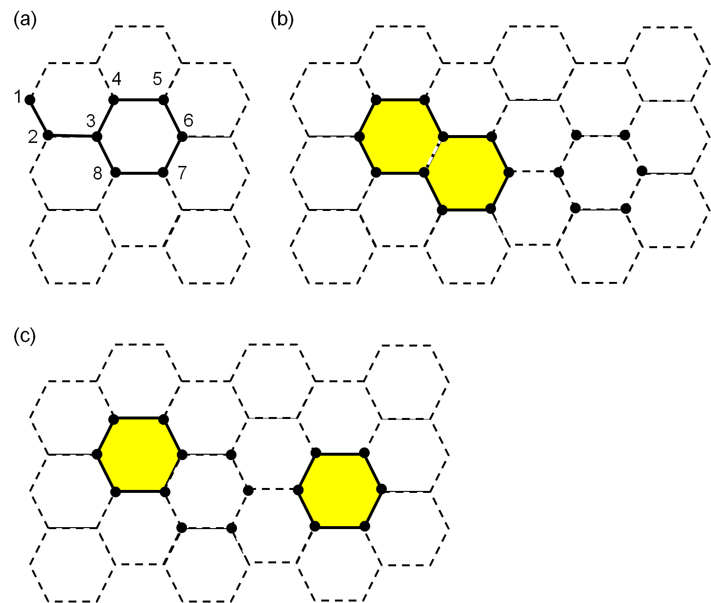
Figure 12: Illustration of loops. (a) A domain consisting of 8 vertices, 8 edges and 1 face. The numbers indicate one possible order in which the domain could be grown. When the first vertex is added, $V=1$, $E=F=0$. As vertices 2 to 7 are added both $V$ and $E$ increase by 1. When the 8${}^{\hbox{th}}$ vertex is added, $V$ and $F$ increase by 1 and $E$ increases by 2. (b) In this domain, which contains $F=3$ faces, two of them are selected, as indicated by shading. The corresponding set of loops is a single loop surrounding the two adjacent faces as indicated by heavy lines. This domain contains $V=16$ vertices and $E=18$ edges, obeying $F=E-V+1$. (c) This is the same domain as in the previous figure (b) but a different subset of faces is selected. Now the set of loops consists of 2 loops as indicated by heavy lines.

Appendix B S=1, 1 dimension

We first consider the 1D S=1 case as a warm-up.

B.1 Open Boundary Conditions

Consider a chain of $n$ spin-1’s on sites $i=1,2,\ldots n$ with 2 additional S=1/2’s at sites 0 and n+1 to remove the “dangling bonds”. Then the AKLT ground state is:

$$|\psi\rangle_{0}=\prod_{i=0}^{n}(a^{\dagger}_{i}b^{\dagger}_{i+1}-a^{\dagger}_{i+1}b^{\dagger}_{i})|0\rangle.$$ (75)

Thus:

$$|\psi_{0}|^{2}=\prod_{i=0}^{n}[1-\hat{\Omega}_{i}\cdot\hat{\Omega}_{i+1}].$$ (76)

We only make projective measurements on the sites containing spin-1’s, at $1,2,\ldots n$. In this case we may replace each factor $1-\hat{\Omega}_{i}\cdot\hat{\Omega}_{j}$ by $1$ because all other terms in the expansion contain a single power of one or more $\hat{\Omega}_{i}$ vector and thus give zero after integrating over $\hat{\Omega}_{i}$. Using:

$$\langle(\Omega^{a})^{2}\rangle=(1/3)\langle(\hat{\Omega})^{2}\rangle=1/3,\ \ \langle(5\Omega^{a})^{2}-1\rangle=2/3,$$ (77)

we obtain a constant:

$$P^{a_{1}a_{2}\ldots a_{n}}=(1/3)^{n}$$ (78)

independent of the $a_{i}$’s.

B.2 Periodic Boundary Conditions

Now we consider $n$ sites, all with spin-1’s and couple site $n$ to site $1$. This is a useful warm up for the 2D case because there is now one closed loop, i.e., one other term in the expansion can give a non-zero integral: $(-1)^{n}\prod_{i=1}^{n}\Omega_{i}\cdot\Omega_{i+1}$. Now we need the integral:

$$\int d\hat{\Omega}[5(\Omega^{a})^{2}-1]\Omega^{b}\Omega^{c}.$$ (79)

Clearly this vanishes unless $b=c$. Note that:

$$\langle(\Omega^{z})^{4}\rangle=\langle\cos^{4}\theta\rangle=(1/2)\int_{-1}^{1}dxx^{4}=1/5$$ (80)

and

$$\langle(\Omega^{x})^{2}(\Omega^{y})^{2}\rangle = \int_{0}^{2\pi}{d\phi\over 2\pi}\cos^{2}\phi\sin^{2}\phi\int_{-1}^{1}{dx\over 2}(1-x^{2})^{2}$$ (81)

$$= 1/15.$$

Thus we obtain the remarkable identity:

$$\langle[5(\Omega^{a})^{2}-1]\Omega^{b}\Omega^{c}\rangle={2\over 3}\delta^{bc}\delta^{ab}.$$ (82)

The integral vanishes unless $a=b=c$ in which case it has the same value as $\langle(5\Omega^{a})^{2}-1\rangle$. The product $(-1)^{n}\prod_{i=1}^{n}\hat{\Omega}_{i}\cdot\hat{\Omega}_{i+1}$ contains sums over $n$ indices. However, for the integrals to be non-zero all $a_{i}$ indices must equal each other. In this case the multiple integral has exactly the same value as when the product is not present, giving:

$$P^{a_{1}a_{2}\ldots a_{n}}=(1/3)^{n}{[1+(-1)^{n}\delta_{a_{1}a_{2}}\delta_{a_{2}a_{3}}\ldots\delta_{a_{n}a_{1}}]\over 1+(-1)^{n}(1/3)^{n-1}}.$$ (83)

Here we have used the fact that the partition function also obtains a contribution from $(-1)^{n}\prod_{i=1}^{n}\Omega_{i}\cdot\Omega_{i+1}$ giving the second term in the denominator and the reason that it is three times larger than $1/3^{n}$ is because of three possibilities $a=x,y,z$, or more precisely,

$$(1/4\pi)^{n}\int\prod_{i=1}^{n}d^{2}\Omega_{i}\,\vec{\Omega}_{i}\cdot\vec{\Omega}_{i+1}=(1/3)^{n-1},$$ (84)

where $\vec{\Omega}_{n+1}\equiv\vec{\Omega}_{1}$. Thus, $P^{a_{1}a_{2}\ldots a_{n}}$ is nearly constant again except that in the one case where $a_{1}=a_{2}=\ldots a_{n}$ it is twice as big if $n$ is even or zero if $n$ is odd. This result agrees precisely with that obtained by other methods in sub-section Sec. II.4.

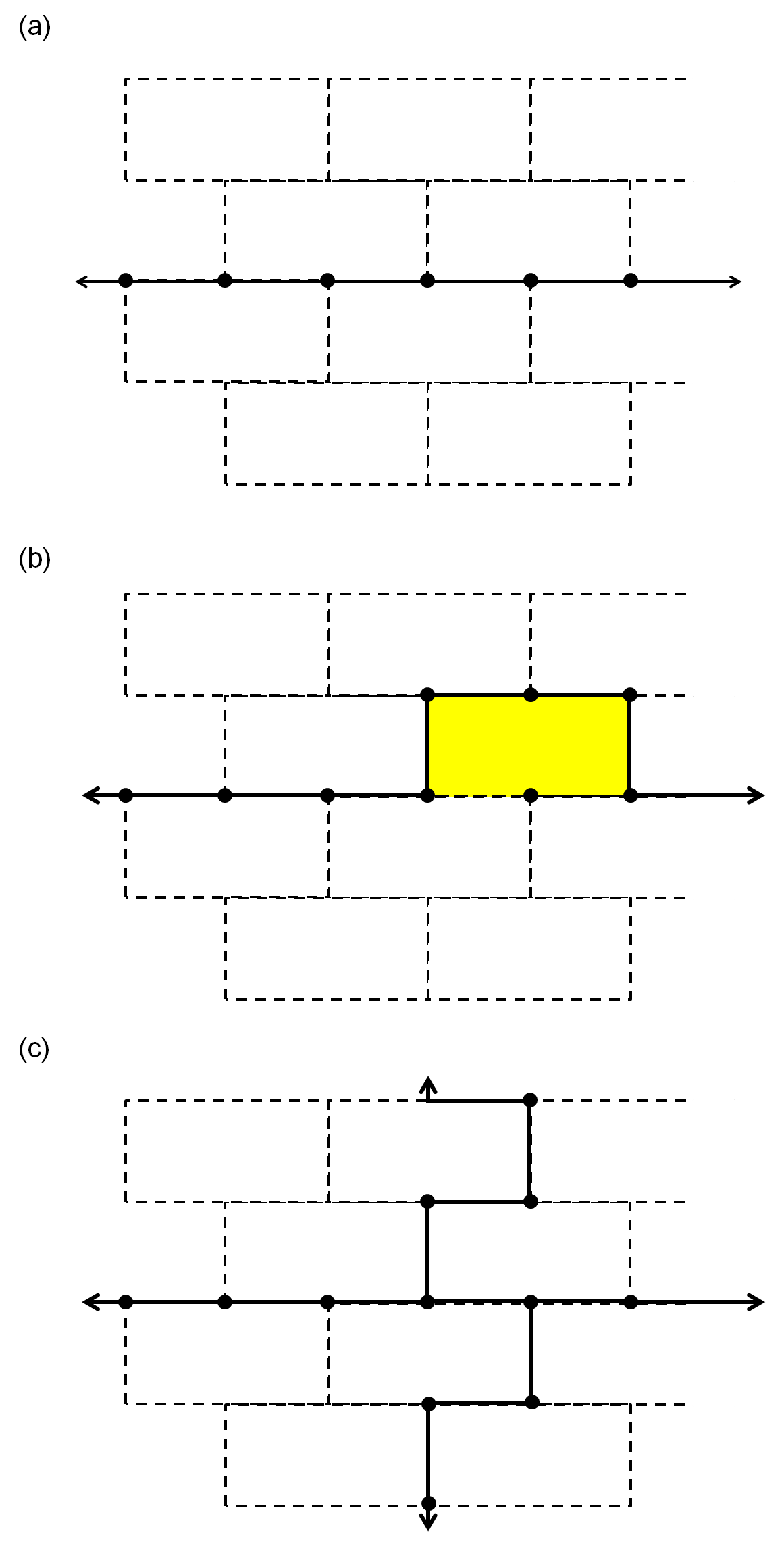
Figure 13: Illustration of loops in the case of the periodic boundary condition. A honeycomb lattice with periodic boundary conditions, drawn as a “brick wall” lattice for convenience. (a) A topological loop is shown. The arrows indicate an edge in the domain between vertices at the left and right hand sides of the lattice. (b) The set of loops (one loop in this case) is shown for a domain containing one topological loop and one face sharing on edge with the topological loop, corresponding to the case in which the face and the topological loop are chosen. (c)A domain containing two topological loops, with $W=2$. It can be seen that there are 3 possible loops, corresponding to 4 sets of loops, and zero faces.

Appendix C S=3/2, 2 dimensions

C.1 Open Boundary Conditions

Consider an arbitrary finite segment of a honeycomb lattice, consisting of $n$ spins; it could have zig-zag and armchair edges or disordered ones, for example. Spins on the boundary will generally be coupled to either 2 or 3 other spins - 2 for a zig-zag edge and 3 for an armchair edge, for example. In all cases where a boundary spin is only coupled to 2 other spins, couple it to a boundary S=1/2 spin. Let the total number of spins, including the S=1/2 spins on the boundary be $M$. Then the square of the AKLT ground state is:

$$|\psi_{0}|^{2}=\prod_{\langle i,j\rangle}[1-\hat{\Omega}_{i}\cdot\hat{\Omega}_{j}].$$ (85)

The product is over all nearest neighbours, as usual including both S=3/2 and S=1/2 spins. We only do the POVM on the S=3/2 spins. Since each of the boundary S=1/2 spins couples to only one other (S=3/2) spin, we may replace $[1-\hat{\Omega}_{i}\cdot\hat{\Omega}_{j}]$ by $1$ for each factor involving an S=1/2 spin in calculating $P^{a_{1}a_{2}\ldots a_{n}}$. Following the above reasoning, when we take the $1$ term in the expansion of $\prod_{\langle i,j\rangle}[1-\hat{\Omega}_{i}\cdot\hat{\Omega}_{j}]$, we get:

$$P^{a_{1}a_{2}\ldots a_{n}}={1\over Z}(4\pi)^{M}(1/3)^{N}(2/3)^{N}+\ldots$$ (86)

There will be many additional terms in this case, unlike the D=1 case. Each additional term must correspond to a set of closed loops on the lattice, with zero or two lines entering each of the S=3/2 sites. These loops never involve the S=1/2 boundary sites. These loops can never cross each other but we can have loops inside loops. Such a contribution only exists when all the $a_{i}$’s for sites on a given loop have the same value. Each such term makes an equal contribution to $P^{a_{1}a_{2}\ldots a_{n}}.$ Thus we simply need to calculate the number of sets of closed loops with equal $a_{i}$’s for a given configuration $a_{1},a_{2},\ldots a_{n}$.

To do this it is convenient to divide up all sites on the lattice into domains such that $a_{i}$ has the same value for all sites in a domain and all sites in a domain are the nearest neighbor of at least one other site in the domain. (Here sites refers to the sites with S=3/2 spins only.) The number of sites in a domain can range from 1 to $n$, in principle, although we expect that typical domains are microscopic. We draw a line between all nearest neighbors in each domain. We may identify a unique number of faces with each domain, $F_{i}$ and a total number of faces, $F=\sum_{i}F_{i}$ with a given configuration. A face, inside a domain, is an elementary hexagon which is completely surrounded by $6$ edges belonging to that domain. Thus, it is impossible to move from the interior of a face to its exterior (either inside the domain or not) without crossing an edge belonging to its domain. The total number of sets of closed loops, $N_{L}$ is then simply

$$N_{L}=2^{F}.$$ (87)

This follows because there is a unique set of loops which surrounds any subset of the faces. See Fig. 12.

The $i^{\hbox{th}}$ domain will also have a number of edges, $E_{i}$ and a number of vertices, $V_{i}$. It can be seen that:

$$F_{i}=E_{i}-V_{i}+1.$$ (88)

This can be seen by induction, growing the domain site by site, always adding new sites which are nearest neighbors of at least one previous site. After drawing the first site, $V_{i}=1$ and $E_{i}=F_{i}=0$, so Eq. (88) is obeyed. When we add the next site, we increase both $E_{i}$ and $V_{i}$ by 1, without changing $F_{i}$. This goes on for a while but we may eventually add a site which is the nearest neighbor of 2 previous sites. At that step, $V_{i}$ increases by 1, $E_{i}$ increases by 2 and $F_{i}$ increases by 1 since we are then closing a loop, making a new face. Thus Eq. (88) remains true at each step as we grow the domain, completing the proof.

Suppose we define a new, random lattice, by collapsing each domain down to one vertex, with an arbitrary number of edges, inherited from the original lattice, connecting the various domains. Let $V^{\prime}$ by the number of vertices of this random lattice and $E^{\prime}$ be the number of edges. (We ignore the S=1/2 boundary spins here.) Then:

$$V^{\prime}=n-\sum_{i}(V_{i}-1)$$ (89)

since $V_{i}$ sites are reduced to 1 at the $i^{\hbox{th}}$ domain. Similarly if $n_{E}$ is the total number of edges connecting S=3/2 spins in the original honeycomb lattice, then

$$E^{\prime}=n_{E}-\sum E_{i}.$$ (90)

Thus:

$$P^{a_{1}a_{2}\ldots a_{n}}\propto 2^{V^{\prime}-E^{\prime}}$$ (91)

the same result obtained in Sec. VI.1 by another method.

C.2 Periodic Boundary Conditions

Now consider a honeycomb lattice of S=3/2’s (no S=1/2’s now) with periodic boundary conditions. This can be done in such a way that every spin has 3 nearest neighbors and we take the AKLT ground state. Similar to the D=1 case, there can now be additional sets of loops because we can form loops that wrap around the torus but don’t correspond to faces; see Fig. 13. If a domain wraps around the torus one way, but not the other, then the total number of sets of loops, corresponding to the domain is:

$$N_{Li}=2^{F_{i}+1}.$$ (92)

To see this choose an arbitrary “topological loop” within the domain going around the torus which doesn’t encircle any faces. There are now 2 sets of loops corresponding to an arbitrary subset of faces, not using this topological loop and the arbitrary subsets of faces together with the topological loop. The construction of the set of loops corresponding to the topological loop plus subset of faces is constructed by analogy with the above construction. In cases where none of the faces share edges with the topological loop the set of loops corresponds to the topological loop plus the loops around the subset of faces. In cases where one or more faces shares an edge with the topological loop, the topological loop is modified to enclose each such face; see Fig. 13b.

Finally, it is possible to have 2 topological loops in a domain, going around the torus the two inequivalent ways; see Fig. 13c. (In this case all other domains must be topologically trivial.) We can grow the domain initially by drawing these 2 topological loops without any faces. At this stage there are 3 closed loops, going around the torus one way or the other or using all edges in the domain to go around both ways. Thus the number of sets of loops is 4 at this stage. After growing the entire domain we how have:

$$N_{Li}=2^{F_{i}+2}$$ (93)

since each set of loops corresponds to a subset of faces, possibly combined with one of these three topological loops. In general, we may associate a winding number with each domain $W_{i}=0$, $1$ or $2$ with:

$$N_{Li}=2^{F_{i}+W_{i}}.$$ (94)

It can be seen that the number of vertices and edges in each domain obeys, in general:

$$F_{i}+W_{i}=E_{i}-V_{i}+1.$$ (95)

This follows by induction, as we grow the domain. At the step when we complete the first topological loop we increase $E_{i}$ by 2 but $V_{i}$ by 1 and $F_{i}$ by 0. Adding further faces respects

$$\Delta F_{i}=\Delta E_{i}-\Delta V_{i}$$ (96)

as before. On the other hand, if we further grow a second topological loop so that the torus is encircled both directions, at the step where it goes around the torus in the second direction we again increase $E_{i}$ by 2 but $V_{i}$ by 1 and $F_{i}$ by 0. Thus Eq. (91) remains true also with periodic boundary conditions.

References

- (1) P. W. Shor, in Proceedings of the 35th Annual Symposium on Foundations of Computer Science, edited by S. Goldwasser (IEEE Computer Society, Los Alamitos, CA, 1994), p. 124.
- (2) M. Nielsen and I. Chuang, Quantum Computation and Quantum Information (Cambridge Univ. Press, 2000).
- (3) E. Farhi, J. Goldstone, S. Gutmann, J. Lapan, A. Lundgren, and D. Preda, Science 292, 472 (2001).
- (4) D. Averin, Solid State Comm. 105, 659 (1998).
- (5) A. M. Childs, Phys. Rev. Lett. 102, 180501 (2009).
- (6) D. Gottesman and I. L. Chuang, Nature (London) 402, 390 (1999).
- (7) M. A. Nielsen, Phys. Lett. A 308, 96 (2003); D. W. Leung, Int. J. Quantum Inform. 2, 33 (2004); A. M. Childs, D. W. Leung, and M. A. Nielsen, Phys. Rev. A 71, 032318 (2005).
- (8) R. Raussendorf and H. J. Briegel, Phys. Rev. Lett. 86, 5188 (2001); R. Raussendorf, D. E. Browne, H. J. Briegel, Phys. Rev. A 68, 022312 (2003).
- (9) H. J. Briegel, D. E. Browne, W. Dür, R. Raussendorf, and M. Van den Nest, Nature Phys. 5, 19 (2009).
- (10) R. Raussendorf and T.-C. Wei, Annual Review of Condensed Matter Physics 3, pp.239-261 (2012).
- (11) M. Van den Nest, A. Miyake, W. Dür, and H. J. Briegel, Phys. Rev. Lett. 97, 150504 (2006).
- (12) D. Gross, S.T. Flammia, and J. Eisert, Phys. Rev. Lett. 102, 190501 (2009).
- (13) H. J. Briegel and R. Raussendorf, Phys. Rev. Lett. 86, 910-913 (2001).
- (14) D. Gross and J. Eisert, hys. Rev. Lett. 98, 220503 (2007); D. Gross, J. Eisert, N. Schuch, and D. Perez-Garcia, Phys. Rev. A 76, 052315 (2007).
- (15) F. Verstraete and J. I. Cirac, Phys. Rev. A 70 060302(R) (2004).
- (16) J.-M. Cai, W. Dür, M. Van den Nest, A. Miyake, and H. J. Briegel, Phys. Rev. Lett. 103, 050503 (2009).
- (17) O. Mandel, M. Greiner, A. Widera, T. Rom, T. W. Hänsch, and I. Bloch, Nature (London) 425, 937 (2003).
- (18) M. A. Nielsen, Rep. Math. Phys. 57, 147 (2005).
- (19) S. D. Bartlett and T. Rudolph, Phys. Rev. A 74, 040302(R) (2006).
- (20) X. Chen, B. Zeng, Z.-C. Gu, B. Yoshida, and I. L. Chuang, “Gapped Two-Body Hamiltonian Whose Unique Ground State Is Universal for One-Way Quantum Computation”, Phys. Rev. Lett. 102, 220501 (2009).
- (21) J.-M. Cai, A. Miyake, W. Dür, and H. J. Briegel, Phys. Rev. A 82, 052309 (2010).
- (22) T.-C. Wei, R. Raussendorf, and L. C. Kwek, Phys. Rev. A 84, 042333 (2011).
- (23) Y. Li, D. E. Browne, L. C. Kwek, R. Raussendorf, and T.-C. Wei, Phys. Rev. Lett. 107, 060501 (2011).
- (24) I. Affleck, T. Kennedy, E. H. Lieb, and H. Tasaki, Phys. Rev. Lett. 59, 799 (1987).
- (25) I. Affleck, T. Kennedy, E. H. Lieb, and H. Tasaki, Comm. Math. Phys. 115, 477 (1988).
- (26) T. Kennedy, E. H. Lieb, and H. Tasaki, J. Stat. Phys. 53, 383-415 (1988).
- (27) F. D. M. Haldane, Phys. Lett. A 93, 464 (1983) and Phys. Rev. Lett. 50, 1153 (1983).
- (28) S. Östlund and S. Rommer, Phys. Rev. Lett. 75, 3537 (1995); M. Fannes, B. Nachtergaele, and R. F. Werner, Commun. Math. Phys. 144, 443 (1992); A. Klümper, A. Schadschneider, and J. Zittartz, J. Phys. A 24, L955 (1991).
- (29) F. Verstraete and J. I. Cirac, eprint cond-mat/0407066 (unpublished); T. Nishino, Y.o Hieida, K. Okunishi, N. Maeshima, Y. Akutsu, and A. Gendiaret, Prog. Theor. Phys. 105, 409 (2001).
- (30) G. K. Brennen and A. Miyake, Phys. Rev. Lett. 101, 010502 (2008).
- (31) J. Lavoie, R. Kaltenbaek, B. Zeng, S. D. Bartlett, and K. J. Resch, Nature Phys. doi:10.1038/nphys1777.
- (32) A. Miyake, Phys. Rev. Lett. 105, 040501 (2010).
- (33) S. D. Bartlett, G. K. Brennen, A. Miyake, and J. M. Renes, Phys. Rev. Lett. 105, 110502 (2010).
- (34) T.-C. Wei, I. Affleck, and R. Raussendorf, Phys. Rev. Lett. 106, 070501 (2011).
- (35) A. Miyake, Ann. Phys. (Leipzig) 326, 1656 (2011).
- (36) A. S. Darmawan, G. K. Brennen, and S. D. Bartlett, New J. Phys. 14, 013023(2012).
- (37) X. Chen, R. Duan, Z. Ji, and B. Zeng, Phys. Rev. Lett. 105, 020502 (2010).
- (38) D. Gottesman, Stabilizer Codes and Quantum Error Correction, Ph.D. Thesis, Caltech (1997); also in e-print arXiv:quant-ph/9705052.
- (39) M. Hein, J. Eisert, and H.-J. Briegel, Phys. Rev. A 69, 062311 (2004).
- (40) R. Durrett, Random Graph Dynamics, Cambridge University Press (2007).
- (41) D. E. Browne, M. B. Elliott, S. T. Flammia, S. T. Merkel, A. Miyake, and A. J Short, New J. Phys. 10, 023010 (2008).
- (42) J. Hoshen and R. Kopelman, Phys. Rev. B 14, 3438-3445 (1976).
- (43) The Betti number of a graph is defined as , and it counts the number of independent cylcles.
- (44) Y. Y. Shi, L. M. Duan, and G. Vidal, Phys. Rev. A 74, 022320 (2006).
- (45) Critical degree bond percolation in 2D lattices. Honeycomb: , Kagome: , square: , triangular: .
- (46) K. Kieling, T. Rudolph, and J. Eisert, Phys. Rev. Lett. 99, 130501 (2007).
- (47) D. P. Arovas, A. Auerbach and F.D.M. Haldane, Phys. Rev. Lett. 60, 531 (1988).