From logarithmic to subdiffusive polynomial fluctuations for internal DLA and related growth models

Abstract

We consider a cluster growth model on ${\mathbb{Z}}^{d}$, called internal diffusion limited aggregation (internal DLA). In this model, random walks start at the origin, one at a time, and stop moving when reaching a site not occupied by previous walks. It is known that the asymptotic shape of the cluster is spherical. When dimension is 2 or more, we prove that fluctuations with respect to a sphere are at most a power of the logarithm of its radius in dimension $d\geq 2$. In so doing, we introduce a closely related cluster growth model, that we call the flashing process, whose fluctuations are controlled easily and accurately. This process is coupled to internal DLA to yield the desired bound. Part of our proof adapts the approach of Lawler, Bramson and Griffeath, on another space scale, and uses a sharp estimate (written by Blachère in our Appendix) on the expected time spent by a random walk inside an annulus.

T1Supported by GDRE 224 GREFI-MEFI, the French Ministry of Education through the ANR BLAN07-2184264 grant, by the European Research Council through the “Advanced Grant” PTRELSS 228032.

and

1 Introduction

The internal DLA cluster of volume $N$, say $A(N)$, is obtained inductively as follows. Initially, we assume that the explored region is empty, that is, $A(0)=\varnothing$. Then, consider $N$ independent discrete-time random walks $S_{1},\ldots,S_{N}$ starting from 0. For $k\leq N$, assume $A(k-1)$ is obtained, and define

$$\tau_{k}=\inf\bigl{\{}{t\geq 0\dvtx S_{k}(t)\notin A(k-1)}\bigr{\}}\quad\mbox{and}\quad A(k)=A(k-1)\cup\bigl{\{}S_{k}(\tau_{k})\bigr{\}}.$$

In such a particle system, we call explorers the particles. We say that the $k$th explorer is settled on $S_{k}(\tau_{k})$ after time $\tau_{k}$, and is unsettled before time $\tau_{k}$. The cluster $A(N)$ consists of the positions of the $N$ settled explorers.

The mathematical model of internal DLA was introduced first in the chemical physics literature by Meakin and Deutch meakin-deutch . There are many industrial processes that look like internal DLA; see the nice review paper landolt . The most important seems to be electropolishing, defined as the improvement of surface finish of a metal effected by making it anodic in an appropriate solution. There are actually two distinct industrial processes (i) anodic leveling or smoothing which corresponds to the elimination of surface roughness of height larger than 1 micron, and (ii) anodic brightening which refers to elimination of surface defects which are protruding by less than 1 micron. The latter phenomenon requires an understanding of atom removal from a crystal lattice. It was noted in meakin-deutch that, at a qualitative level, the model produces smooth clusters, and the authors wrote, “it is also of some fundamental significance to know just how smooth a surface formed by diffusion limited processes may be.”

Diaconis and Fulton diaconis-fulton introduced internal DLA in mathematics. They allowed explorers to start on distinct sites, and showed that the law of the cluster was invariant under permutation of the order in which explorers were launched. This invariance, named the abelian property, was central in their motivation. They treat, among other things, the special one-dimensional case.

In dimension two or more, Lawler, Bramson and Griffeath lawler92 prove that in order to cover, without holes, a sphere of radius $n$, we need about the number of sites of ${\mathbb{Z}}^{d}$ contained in this sphere. In other words, the asymptotic shape of the cluster is a sphere. Then, Lawler in lawler95 shows subdiffusive fluctuations. The latter result is formulated in terms of inner and outer errors, which we now introduce with some notation. We denote with $\|\cdot\|$ the Euclidean norm on ${\mathbb{R}}^{d}$. For any $x$ in ${\mathbb{R}}^{d}$ and $r$ in ${\mathbb{R}}$, set

$$B(x,r)=\bigl{\{}y\in{\mathbb{R}}^{d}\dvtx\|y-x\|<r\bigr{\}}\quad\mbox{and}\quad{\mathbb{B}}(x,r)=B(x,r)\cap{\mathbb{Z}}^{d}.$$

For $\Lambda\subset{\mathbb{Z}}^{d}$, $|\Lambda|$ denotes the number of sites in $\Lambda$. The inner error $\delta_{I}(n)$ is such that

$$n-\delta_{I}(n)=\sup\bigl{\{}{r\geq 0\dvtx{\mathbb{B}}(0,r)\subset A\bigl{(}\bigl{|}{\mathbb{B}}(0,n)\bigr{|}\bigr{)}}\bigr{\}}.$$

Also, the outer error $\delta_{O}(n)$ is such that

$$n+\delta_{O}(n)=\inf\bigl{\{}{r\geq 0\dvtx A\bigl{(}\bigl{|}{\mathbb{B}}(0,n)\bigr{|}\bigr{)}\subset{\mathbb{B}}(0,r)}\bigr{\}}.$$

The main result of lawler95 reads as follows.

Theorem 1.1 ((Lawler))

Assume $d\geq 2$. Then

$$P\bigl{(}{\exists n(\omega)\dvtx\forall n\geq n(\omega)\ \delta_{I}(n)\leq n^{1/3}\log(n)^{2}}\bigr{)}=1$$ (1)

and

$$P\bigl{(}{\exists n(\omega)\dvtx\forall n\geq n(\omega)\ \delta_{O}(n)\leq n^{1/3}\log(n)^{4}}\bigr{)}=1.$$ (2)

Since Lawler’s paper, published 15 years ago, no improvement of these estimates was achieved, but it is believed that fluctuations are on a much smaller scale than $n^{1/3}$. Moreover, (1) and (2) are almost sure upper bounds on errors, and no lower bound on the inner or outer error has been established. Computer simulations machta-moore , levine suggest indeed that fluctuations are logarithmic. In addition, Levine and Peres studied a deterministic analogue of internal DLA, the rotor-router model, introduced by Propp kleber-propp . They bound, in levine-peres , the inner error $\delta_{I}(n)$ by $\log(n)$, and the outer error $\delta_{O}(n)$ by $n^{1-1/d}$.

Our main result is the following improvement of Theorem 1.1.

Theorem 1.2

Assume $d\geq 2$. There is a positive constant $A_{d}$ such that

$$P\bigl{(}{\exists n(\omega)\dvtx\forall n\geq n(\omega)\ \delta_{I}(n)\leq A_{d}\log(n)}\bigr{)}=1$$ (3)

and

$$P\bigl{(}{\exists n(\omega)\dvtx\forall n\geq n(\omega)\ \delta_{O}(n)\leq A_{d}\log^{2}(n)}\bigr{)}=1.$$ (4)

Note added in proof. At about the same time, and with an independent approach, Jerison, Levine and Sheffield JLS1 obtained similar results with an improved bound on the outer error in $d=2$. Then, by refining our approach, we obtained in AG2 a bound of order $\sqrt{\log(n)}$ for both internal and external errors in dimension three or more. Jerison, Levine and Sheffield JLS2 did the same by following their approach.

Our approach builds on the work of Lawler, Bramson and Griffeath lawler92 , which we review later. It also deals with more general models of diffusion limited aggregation which we now describe. Indeed, we introduce a family of cluster growth models for which a control of the fluctuations of the cluster shape is easily obtained. These growth models are built so that the asymptotic shape is spherical, but still they exhibit a large diversity of fluctuations parametrized by a certain width ranging from a large constant to a power $1/3$ of the radius of the asymptotic sphere. Moreover, all these clusters are coupled to internal DLA, and, as a consequence, we obtain logarithmic bounds on the fluctuations for internal DLA. We generalize internal DLA by allowing explorers to settle only at some special times. Thus, each explorer $i$ is associated with a collection of times $\{\sigma_{i,k},k\in{\mathbb{N}}\}$ and

$$\tau_{i}^{*}=\inf\bigl{\{}{\sigma_{i,k}\dvtx S_{i}(\sigma_{i,k})\notin A^{*}(i-1)}\bigr{\}}\quad\mbox{and}\quad A^{*}(i)=A^{*}(i-1)\cup\bigl{\{}S_{i}\bigl{(}\tau_{i}^{*}\bigr{)}\bigr{\}}.$$

The internal DLA is recovered as we choose $\sigma_{i,k}=k$ for all $i=1,\ldots,N$ and $k\in{\mathbb{N}}$. We call $\{\sigma_{i,k},k\in{\mathbb{N}}\}$ the flashing times associated to the $i$th explorer, and $\{S_{i}(\sigma_{i,k}),k\in{\mathbb{N}}\}$ its flashing positions.

In this paper, we consider stopping times of a special form, linked with the spherical nature of the internal DLA cluster. An illustration with one flashing explorer’s trajectory is made in Figure 1.

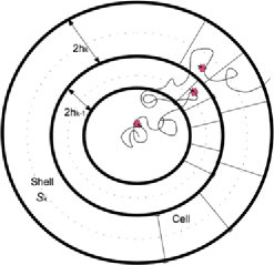
Figure 1: Cell decomposition, and flashing positions as stars.

The precise definition of the flashing times requires additional notation, which we postpone to Section 3. We describe here key features of flashing processes. We first choose a sequence of widths, say ${\cal{H}}=\{h_{n},n\in{\mathbb{N}}\}$, and then partition ${\mathbb{Z}}^{d}$ into concentric shells $\{{\cal{S}}_{n},n\in{\mathbb{N}}\}$, whose respective widths are $\{2h_{n},n\in{\mathbb{N}}\}$. Each shell is in turn partitioned into cells, which are brick-like domain, of side length equal to the width of the shell. The flashing times are chosen such that (i) an explorer flashes at most once in each shell, (ii) the flashing position, in a shell, is essentially uniform over the cell an explorer first hits upon entering the shell and (iii) when an explorer leaves a shell, it cannot afterward flash in it.

For a given sequence ${\cal{H}}$, we call the process just described the ${\cal{H}}$-flashing process. Note that feature (ii) is the seed of a deep difference with internal DLA. The mechanism of covering a cell, for the flashing process, is very much the same as completing an album in the classical coupon-collector process. Thus, we need of the order of $V\log(V)$ explorers to cover a cell of volume $V$. For internal DLA, with explorers started at the origin, we only need of order $V$ explorers to cover a sphere of volume $V$ as shown in lawler92 , and we believe that we need a number of explorers of order $|{\cal C}|$ to cover a cell ${\cal C}$, even if they start on the boundary of the cell. In addition, feature (ii) allows us to localize the covering mechanism, in the sense that a particle entering a shell cannot flash outside the cell through which it entered that shell. Finally, feature (iii) is essential for having a useful coupling between flashing and internal DLA processes.

Lemma 1.3

Assume that $N$ is an integer, and ${\cal{H}}$ is a sequence of positive integers. There is a coupling between the two processes, using the same trajectories $S_{1},\ldots,S_{N}$ such that

$$A(N)=\bigcup_{i=1}^{N}\bigl{\{}S_{i}\bigl{(}T(i)\bigr{)}\bigr{\}}\quad\mbox{and}\quad A^{*}(N)=\bigcup_{i=1}^{N}\bigl{\{}S_{i}\bigl{(}T^{*}(i)\bigr{)}\bigr{\}}$$ (5)

and $T^{*}(i)\geq T(i)$ for all $i=1,\ldots,N$.

As a corollary of Lemma 1.3, we have the following useful result.

Corollary 1.4

Under the hypotheses of the previous lemma, for $k\geq 1$:

• if $A^{*}(N)\subset\bigcup_{j<k}{\cal{S}}_{j}$, then $A(N)\subset\bigcup_{j<k}{\cal{S}}_{j}$;

• if $\bigcup_{j<k}{\cal{S}}_{j}\subset A^{*}(N)$, then $\bigcup_{j<k}{\cal{S}}_{j}\subset A(N)$.

An ${\cal{H}}$-flashing process, with $h_{j}\geq h_{0}$ for $j\geq 0$, and $h_{0}$ a large constant, produces a cluster $A^{*}(N)$, for which we bound easily the inner error, $\delta^{*}_{I}(n)$. Then, to bound the outer error, $\delta^{*}_{O}(n)$, we follow the approach of lawler95 , though with a slightly simpler proof.

Proposition 1.5

Assume that for $j\geq 1$, $h_{j}\leq h_{j+1}\leq(1+\frac{1}{2j})h_{j}$, with a large $h_{0}$. For a positive constant $A_{d}^{*}$, we have

$$P\bigl{(}{\exists n(\omega)\dvtx\forall n\geq n(\omega)\ \delta^{*}_{I}(n)\leq A_{d}^{*}h(n)\log(n)}\bigr{)}=1$$ (6)

and

$$P\bigl{(}{\exists n(\omega)\dvtx\forall n\geq n(\omega)\ \delta^{*}_{O}(n)\leq A_{d}^{*}h(n)\log^{2}(n)}\bigr{)}=1,$$ (7)

where $h(n)=\max\{h_{k}\in{\mathbb{R}}\dvtx r_{k}\leq n\}$.

Finally, we establish lower bound on the inner and outer error.

Proposition 1.6

Assume that $h_{0}$ is large enough. Then, there is a constant $a_{d}^{*}$ such that

$$P\bigl{(}{\exists n(\omega)\dvtx\forall n\geq n(\omega)\ \delta^{*}_{I}(n)\geq a_{d}^{*}h(n)\log\bigl{(}h(n)\bigr{)}}\bigr{)}=1$$ (8)

and

$$P\bigl{(}{\exists n(\omega)\dvtx\forall n\geq n(\omega)\ \delta^{*}_{O}(n)\geq a_{d}^{*}h(n)\log(n)}\bigr{)}=1.$$ (9)

Corollary 1.4 and Proposition 1.5, with the choice $h_{j}=h_{0}$ for all $j>0$, imply Theorem 1.2 which deals with internal DLA.

Let us now review previous work on internal DLA.

On previous bounds for internal DLA

We describe the approach of lawler92 , for establishing the upper bound for the inner error. It is convenient to consider explorers starting outside the origin with initial configuration denoted $\eta$. We denote also by $A(\Lambda,\eta)$ the cluster obtained from explorers initially on $\eta$, with an explored region $\Lambda\subset{\mathbb{Z}}^{d}$.

Now, for a site $z\in{\mathbb{Z}}^{d}$, we call $W(\eta,z)$ [resp., $M(\eta,z)$] the number of explorers (resp., of random walks) which visit $z$ before settling. For an integer $n$, and $\eta$ consisting of $|{\mathbb{B}}(0,n)|$ explorers at the origin, the authors of lawler92 first write

$$\bigl{\{}{{\mathbb{B}}(0,r)\not\subset A(\varnothing,\eta)}\bigr{\}}\subset\bigcup_{z\in{\mathbb{B}}(0,r)}\bigl{\{}{W(\eta,z)=0}\bigr{\}}.$$

Then, they look for the largest value of $r_{n}$ (in terms of $n$) which guarantees that $|{\mathbb{B}}(0,r_{n})|\times\sup_{z\in{\mathbb{B}}(0,r_{n})}P(W(\eta,z)=0)$ be the term of a convergent series.

The approach of lawler92 is based on the following observations. (i) If explorers would not settle, they would just be independent random walks; (ii) exactly one explorer occupies each site of the cluster. Thus, the following equality holds in law:

$$W(\eta,z)+M\bigl{(}A(\varnothing,\eta),z\bigr{)}\geq M(\eta,z).$$

Now, an observation of Diaconis and Fulton diaconis-fulton is that we can realize the cluster by sending many exploration waves. Let us illustrate this observation with two waves. We first stop the explorers on the external boundary of a ball of radius $R$, say $\partial{\mathbb{B}}(0,R)$. The cluster consisting of the positions of settled explorers is denoted $A_{R}(\varnothing,\eta)$, so that $A_{R}(\varnothing,\eta)\subset{\mathbb{B}}(0,R)$. The configuration with stopped explorers on $\partial{\mathbb{B}}(0,R)$ is denoted $\zeta_{R}(\eta)$. Then, the second wave consists in launching the explorers of $\zeta_{R}(\eta)$, with explored region $A_{R}(\varnothing,\eta)$. In other words, we have an equality in law

$$A(\varnothing,\eta)=A_{R}(\varnothing,\eta)\cup A\bigl{(}{A_{R}(\varnothing,\eta),\zeta_{R}(\eta)}\bigr{)}.$$

Moreover, if the index $R$ refers only to explorers (or walks) of the first wave, then for $z\in{\mathbb{B}}(0,R)$,

$$W_{R}(\eta,z)+M_{R}\bigl{(}A_{R}(\varnothing,\eta),z\bigr{)}\geq M_{R}(\eta,z).$$ (10)

The authors of lawler92 consider $R=n$ and $z\in{\mathbb{B}}(0,n)$. Since $W(\eta,z)\geq W_{n}(\eta,z)$, we have using (10), for any $\alpha>0$,

$$P\bigl{(}{W({\eta,z})=0}\bigr{)}\leq P\bigl{(}{M_{n}({\eta,z})<\alpha}\bigr{)}+P\bigl{(}{M_{n}\bigl{(}{{\mathbb{B}}(0,n),z}\bigr{)}>\alpha}\bigr{)}.$$ (11)

We then look for sites $z$ such that $E[M_{n}(\eta,z)]>\alpha>E[M_{n}({\mathbb{B}}(0,n),z)]$ (and $\eta=|\mathbb{B}(0,n)|\delta_{0}$). Note that $M_{n}(\eta,z)$ and $M_{n}({\mathbb{B}}(0,n),z)$ are sums of independent Bernoulli variables with well-known large deviation estimates. If we set

$$2\alpha=E\bigl{[}M_{n}(\eta,z)\bigr{]}+E\bigl{[}M_{n}\bigl{(}{\mathbb{B}}(0,n),z\bigr{)}\bigr{]}$$

and

$$\tilde{\mu}_{n}(z)=E\bigl{[}M_{n}(\eta,z)\bigr{]}-E\bigl{[}M_{n}\bigl{(}{\mathbb{B}}(0,n),z\bigr{)}\bigr{]},$$

then

$$P\bigl{(}{M_{n}(\eta,z)<\alpha}\bigr{)} \leq \exp\biggl{(}{-\frac{(E[M_{n}(\eta,z)]-\alpha)^{2}}{2E[M_{n}(\eta,z)]}}\biggr{)}$$

$$\leq \exp\biggl{(}{-\frac{\tilde{\mu}_{n}^{2}(z)}{8E[M_{n}(\eta,z)]}}\biggr{)}.$$

Lawler in lawler95 establishes that for $z\in{\mathbb{B}}(0,n)$,

$$E\bigl{[}{M_{n}(\eta,z)}\bigr{]}\sim n\bigl{(}n-\|z\|\bigr{)}\quad\mbox{and}\quad\tilde{\mu}_{n}(z)\sim\bigl{(}{n-\|z\|}\bigr{)}^{2}.$$

Replacing these values in (1), the bound $n-\|z\|\geq n^{1/3}\log(n)$ is such that $P(W_{n}(\eta,z)=0)$ is the term of a convergent series.

We now sketch our main ideas leading to logarithmic fluctuations for internal DLA.

On logarithmic fluctuations

Our approach is inspired by Lawler, Bramson and Griffeath’s work lawler92 . We develop three original ideas: (i) we propose a cluster growth model, the flashing process, whose covering mechanism is simpler than internal DLA; (ii) we look at an intermediary scale, the scale of cells, since the deviations of the number of visits decrease with the cell-length; (iii) we build a coupling between flashing process and internal DLA which allows us to transport bounds from one model to the other.

Let us describe how the idea of an intermediary scale is used in the context of flashing processes. Recall that we first partition ${\mathbb{Z}}^{d}$ into a sequence of concentric shells. Each shell is partitioned into cells whose side length equals the width of the shell. Now, we observe that a site has good chances to lie inside the cluster if some cell, say ${\cal{C}}$, about this site, is crossed by many explorers. The notation $W(\eta,{\cal{C}})$ refers to the number of explorers visiting ${\cal{C}}$, when their initial configuration is $\eta$. We drop the index $n$ appearing in $W_{n}(\eta,z)$ since there are no more constraints on not escaping the ball ${\mathbb{B}}(0,n)$. Now, the coupon-collector nature of the covering mechanism suggests that for some positive constant $\alpha_{d}$,

$$W(\eta,{\cal{C}})\geq\alpha_{d}|{\cal{C}}|\times\log\bigl{(}|{\cal{C}}|\bigr{)}$$

(13)

$$\qquad\Longrightarrow\quad{\cal{C}}\subset A(\varnothing,\eta)\mbox{ with a large probability.}$$

We neglect in these heuristics the $\log(|{\cal{C}}|)$ term in (1).

Note that in lawler92 , all the explorers start from the origin, whereas here, we only know that they cross ${\cal{C}}$. For internal DLA, estimating the probability that ${\cal{C}}$ is not covered, when ${\cal{C}}$ is large and $W(\eta,{\cal{C}})\geq\alpha_{d}|{\cal{C}}|$ raises a difficulty which is absent when considering flashing processes.

We now make our argument more precise. For a scale $h$ and an integer $K>1$, to be determined, assume that ${\mathbb{B}}(0,n-Kh)$ is covered by settled explorers. Partition the shell ${\cal{S}}={\mathbb{B}}(0,n-(K-1)h)\setminus{\mathbb{B}}(0,n-Kh)$ into about $(n/h)^{d-1}$ cells, each of volume $h^{d}$. It is also convenient to stop the explorers as they reach the boundary of ${\mathbb{B}}(0,n-Kh)$. Thus, with such a stopped process, explorers are either settled inside ${\mathbb{B}}(0,n-Kh)$ or unsettled but stopped on its boundary, denoted $\partial{\mathbb{B}}(0,n-Kh)$. What we have called earlier the number of explorers crossing ${\cal{C}}$ is taken here to be the unsettled explorers stopped on ${\cal{C}}\cap\partial{\mathbb{B}}(0,n-Kh)$.

Assuming (1) holds, it remains to show that the probability of the event $\{\exists{\cal{C}}\in{\cal{S}}\dvtx W(\eta,{\cal{C}})<\alpha_{d}|{\cal{C}}|\}$ is small. We improve (11) by first using the independence between $W(\eta,{\cal{C}})$ and $M({\mathbb{B}}(0,n-Kh),{\cal{C}})$, and then by replacing $A_{R}(\varnothing,\eta)$ by ${\mathbb{B}}(0,n-Kh)$ in (10) with $R=n-Kh$ and $\eta=|{\mathbb{B}}(0,n)|{\mathbh 1}_{0}$,

$$W(\eta,{\cal{C}})+M\bigl{(}{\mathbb{B}}(0,n-Kh),{\cal{C}}\bigr{)}\geq M(\eta,{\cal{C}}).$$ (14)

Also, we define

$$\mu({\cal{C}})=E\bigl{[}M(\eta,{\cal{C}})\bigr{]}-E\bigl{[}M\bigl{(}{\mathbb{B}}(0,n-Kh),{\cal{C}}\bigr{)}\bigr{]}.$$

Now, using that $M(\eta,z)$ and $M({\mathbb{B}}(0,n-Kh),z))$ are sums of independent Bernoulli variables, we show that (14) implies a Gaussian-type lower tail

$$P\bigl{(}{W(\eta,{\cal{C}})<\alpha_{d}|{\cal{C}}|}\bigr{)}\leq\exp\biggl{(}{-\frac{({\mu({\cal{C}})-\alpha_{d}|{\cal{C}}|})^{2}}{c\nu({\cal{C}})}}\biggr{)}$$ (15)

for a positive constant $c$, and where $\nu({\cal{C}})$

$$\nu({\cal{C}})=\operatorname{var}\bigl{(}{M(\eta,{\cal{C}})}\bigr{)}-\operatorname{var}\bigl{(}{M\bigl{(}{\mathbb{B}}(0,n-Kh),{\cal{C}}\bigr{)}}\bigr{)}.$$

We then show that both $\mu({\cal{C}})$ and $\nu({\cal{C}})$ are of order $K|{\cal{C}}|$. Then, $P(W(\eta,{\cal C})<\alpha_{d}|{\cal C}|)$ is summable as soon as $K|{\cal{C}}|\geq A\log(n)$.

Outline of the paper

The rest of the paper is organized as follows. Section 2 introduces the main notation, and recalls known useful facts. In Section 3, we build the flashing process, give an alternative construction through exploration waves and sketch the proof of Lemma 1.3. In Section 4, we prove Propositions 1.5 and 1.6 using the construction in terms of exploration waves. In Section 5, we obtain a sharp estimate on the expected number of explorers crossing a given cell, and prove feature (ii) of the flashing times. Both proofs are based on classical potential theory estimates. Finally, in the Appendix, we give a proof of Lemma 1.3, and recall a result of Sébastien Blachère.

2 Notation and useful tools

2.1 Notation

We say that $z,z^{\prime}\in{\mathbb{Z}}^{d}$ are nearest neighbors when $\|z-z^{\prime}\|=1$, and we write $z\sim z^{\prime}$. For any subset $\Lambda\subset{\mathbb{Z}}^{d}$, we define

$$\partial\Lambda=\bigl{\{}{z\in{\mathbb{Z}}^{d}\setminus\Lambda\dvtx\exists z^{\prime}\in\Lambda,z^{\prime}\sim z}\bigr{\}}.$$

For any $r\leq R$, we define the annulus

$$A(r,R)=B(0,R)\setminus B(0,r)\quad\mbox{and}\quad{\mathbb{A}}(r,R)=A(r,R)\cap{\mathbb{Z}}^{d}.$$ (16)

A trajectory $S$ is a discrete nearest-neighbor path on ${\mathbb{Z}}^{d}$. That is, $S\dvtx{\mathbb{N}}\to{\mathbb{Z}}^{d}$ with $S(t)\sim S(t+1)$ for all integer $t$. For a subset $\Lambda$ in ${\mathbb{Z}}^{d}$, and a trajectory $S$, we define the hitting time of $\Lambda$ as

$$H(\Lambda;S)=\min\bigl{\{}t\geq 0\dvtx S(t)\in\Lambda\bigr{\}}.$$

We often omit $S$ in the notation when no confusion is possible. We use the shorthand notation

$$B_{n}=B(0,n),\qquad{\mathbb{B}}_{n}={\mathbb{B}}(0,n),\qquad H_{R}=H\bigl{(}B_{R}^{c}\bigr{)}\quad\mbox{and}\quad H_{z}=H\bigl{(}\{z\}\bigr{)}.$$

For any $a$, $b$ in ${\mathbb{R}}$ we write $a\wedge b=\min\{a,b\}$, and $a\vee b=\max\{a,b\}$. Let $\Gamma$ be a finite collection of trajectories on ${\mathbb{Z}}^{d}$. For $R>0$, $z$ in ${\mathbb{Z}}^{d}$ and $\Lambda$ a subset of ${\mathbb{Z}}^{d}$, we call $M(\Gamma,R,z)$ [resp., $M(\Gamma,R,\Lambda)$] the number of trajectories which exit ${\mathbb{B}}(0,R)$ on $z$ (resp., in $\Lambda$).

$$M(\Gamma,R,z)=\sum_{S\in\Gamma}{\mathbf{1}}_{\{S(H_{R})=z\}}\quad\mbox{and}\quad M(\Gamma,R,\Lambda)=\sum_{z\in\Lambda}M(\Gamma,R,z).$$

When we deal with a collection of independent random trajectories, we rather specify its initial configuration $\eta\in{\mathbb{N}}^{{\mathbb{Z}}^{d}}$, so that $M(\eta,R,z)$ is the number of random walks starting from $\eta$ and hitting ${\mathbb{B}}(0,R)^{c}$ on $z$. Two types of initial configurations are important here: (i) the configuration $n{\mathbf{1}}_{z^{*}}$ formed by $n$ walkers starting on a given site $z^{*}$ and (ii) for $\Lambda\subset{\mathbb{Z}}^{d}$, the configuration ${\mathbf{1}}_{\Lambda}$ that we simply identify with $\Lambda$. For any configuration $\eta\in{\mathbb{N}}^{{\mathbb{Z}}^{d}}$ we write

$$|\eta|=\sum_{z\in{\mathbb{Z}}^{d}}\eta(z).$$

For any $\Lambda\subset{\mathbb{Z}}^{d}$, we define Green’s function restricted to $\Lambda$, $G_{\Lambda}$, as follows. For $x,y\in\Lambda$, the expectation with respect to the law of the simple random walk started at $x$, is denoted with ${\mathbb{E}}_{x}$ (the law is denoted ${\mathbb{P}}_{x}$) and

$$G_{\Lambda}(x,y)={\mathbb{E}}_{x}\biggl{[}\sum_{0\leq n<H(\Lambda^{c})}{\mathbf{1}}_{\{S(n)=y\}}\biggr{]}.$$

In dimension 3 or more, Green’s function on the whole space is well defined and denoted $G$. That is, for any $x,y\in{\mathbb{Z}}^{d}$,

$$G(x,y)={\mathbb{E}}_{x}\biggl{[}\sum_{n\geq 0}{\mathbf{1}}_{\{S(n)=y\}}\biggr{]}.$$

In dimension 2, the potential kernel plays the role of Green’s function

$$a(x,y)=\lim_{n\to\infty}{\mathbb{E}}_{x}\Biggl{[}{\sum_{l=0}^{n}\bigl{(}{\mathbf{1}}\bigl{\{}{S(l)=x}\bigr{\}}-{\mathbf{1}}\bigl{\{}{S(l)=y}\bigr{\}}\bigr{)}}\Biggr{]}.$$

2.2 Some useful tools

We recall here some well-known facts. Some of them are proved for the reader’s convenience. This section can be skipped at a first reading.

In lawler92 , the authors emphasized the fact that the spherical limiting shape of internal DLA was intimately linked to strong isotropy properties of Green’s function. This isotropy is expressed by the following asymptotics (Theorem 4.3.1 of lawler-limic ). In $d\geq 3$, there is a constant $K_{g}$, such that for any $z\not=0$,

$$\biggl{|}G(0,z)-\frac{C_{d}}{\|z\|^{d-2}}\biggr{|}\leq\frac{K_{g}}{\|z\|^{d}}\qquad\mbox{with }C_{d}=\frac{2}{v_{d}(d-2)},$$ (17)

where $v_{d}$ stands for the volume of the Euclidean unit ball in ${\mathbb{R}}^{d}$. The first order expansion (17) is proved in lawler-limic for general symmetric walks with finite $d+3$ moments and vanishing third moment. All the estimates we use are eventually based on (17), and we emphasize the fact that the estimate is uniform in $\|z\|$. There is a similar expansion for the potential kernel. Theorem 4.4.4 of lawler-limic establishes that for $z\not=0$ (with $\gamma$ the Euler constant),

$$\biggl{|}a(0,z)-\frac{2}{\pi}\log\bigl{(}{\|z\|}\bigr{)}-\frac{2\gamma+\log(8)}{\pi}\biggr{|}\leq\frac{K_{g}}{\|z\|^{2}}.$$ (18)

We recall a rough but useful result about the exit site distribution from a sphere. This is Lemma 1.7.4 of lawler .

Lemma 2.1

There are two positive constants $c_{1},c_{2}$ such that for any $z\in\partial B(0,n)$, and $n>0$

$$\frac{c_{1}}{n^{d-1}}\leq{\mathbb{P}}_{0}\bigl{(}S(H_{n})=z\bigr{)}\leq\frac{c_{2}}{n^{d-1}}.$$ (19)

We now state an elementary lemma.

Lemma 2.2

Each $z^{*}$ in ${\mathbb{Z}}^{d}\setminus\{0\}$ has a nearest-neighbor $z$ (i.e., $z^{*}\sim z$) such that

$$\|z\|\leq\bigl{\|}z^{*}\bigr{\|}-\frac{1}{2\sqrt{d}}.$$ (20)

Without loss of generality we can assume that all the coordinates of $z^{*}$ are nonnegative. Let us denote by $b$ the maximum of these coordinates, and note that

$$\bigl{\|}z^{*}\bigr{\|}^{2}\leq db^{2}\quad\mbox{and}\quad b\geq 1.$$ (21)

Denote by $z$ the nearest-neighbor obtained from $z^{*}$ by decreasing by one unit a maximum coordinate. Using (21),

$$\bigl{\|}z^{*}\bigr{\|}^{2}-\|z\|^{2}=b^{2}-(b-1)^{2}=2b-1\geq b\geq\frac{\|z^{*}\|}{\sqrt{d}}.$$ (22)

Note that (20) follows from $2\|z^{*}\|(\|z^{*}\|-\|z\|)\geq\|z^{*}\|^{2}-\|z\|^{2}$, and (22).

We state now a handy estimate dealing with sums of independent Bernoulli variables.

Lemma 2.3

Let $\{X_{n},Y_{n},n\in{\mathbb{N}}\}$ be independent 0–1 Bernoulli variables. For integers $n,m$ let $S=X_{1}+\cdots+X_{n}$ and $S^{\prime}=Y_{1}+\cdots+Y_{m}$. Define for $t\in{\mathbb{R}}$

$$f(t)=e^{t}-1-t\quad\mbox{and}\quad g(t)=\bigl{(}{e^{t}-1}\bigr{)}^{2}.$$

If $0\leq t\leq\log(2)$, then

$$\frac{E[{\exp({t({S-E[S]})})}]}{E[{\exp({t({S^{\prime}-E[S^{\prime}]})})}]}\leq\exp\Biggl{(}{f(t)E\bigl{[}{S-S^{\prime}}\bigr{]}+g(t)\sum_{i=1}^{m}E[Y_{i}]^{2}}\Biggr{)}.$$ (23)

Assume now that for $\kappa>1$, $\sup_{n}E[Y_{n}]\leq\frac{\kappa-1}{\kappa}$. If $t\leq 0$, then

$$\quad\frac{E[{\exp({t({S-E[S]})})}]}{E[{\exp({t({S^{\prime}-E[S^{\prime}]})})}]}\leq\exp\Biggl{(}{f(t)E\bigl{[}{S-S^{\prime}}\bigr{]}+\frac{\kappa}{2}g(t)\sum_{i=1}^{m}E[Y_{i}]^{2}}\Biggr{)}.$$ (24)

Let $X$ be a Bernoulli variable, and $p=E[X]$. Using the inequality $e^{x}\geq 1+x$ for $x\in{\mathbb{R}}$, we have

$$E\bigl{[}{\exp\bigl{(}{t\bigl{(}X-E[X]\bigr{)}}\bigr{)}}\bigr{]} = pe^{t(1-p)}+(1-p)e^{-tp}$$

$$= e^{-pt}\bigl{(}{1+p\bigl{(}e^{t}-1\bigr{)}}\bigr{)}$$

$$\leq \exp\bigl{(}{f(t)E[X]}\bigr{)}.$$

For a lower bound, we distinguish two cases.

First, assume $t\geq 0$. We claim that $\exp(x-x^{2})\leq 1+x$ for $0\leq x\leq 1$. Indeed, we use three obvious inequalities: $e^{x}\geq 1+x$ for $x\in{\mathbb{R}}$, (i) for $x\leq 1$, $1+x+x^{2}\geq e^{x}$, and (ii) $(1+x^{2})(1+x)\geq 1+x+x^{2}$. Thus

$$e^{x^{2}}(1+x)\geq\bigl{(}1+x^{2}\bigr{)}(1+x)\geq 1+x+x^{2}\geq e^{x}.$$

This yields the claim. Now, set $x=p(e^{t}-1)$, so that $x\leq 1$ when $e^{t}\leq 2$. The last inequality in (2.2) yields

$$E\bigl{[}{\exp\bigl{(}{t\bigl{(}X-E[X]\bigr{)}}\bigr{)}}\bigr{]} \geq \exp\bigl{(}{-tp+p\bigl{(}e^{t}-1\bigr{)}-p^{2}\bigl{(}e^{t}-1\bigr{)}^{2}}\bigr{)}$$

$$= e^{f(t)p-g(t)p^{2}}.$$

Assume now that $t\leq 0$, and for $\kappa>1$, $p<\frac{\kappa-1}{\kappa}$. We claim that for $0\leq x\leq\frac{\kappa-1}{\kappa}$,

$$\exp\biggl{(}{-x-\frac{\kappa}{2}x^{2}}\biggr{)}\leq 1-x.$$ (27)

Indeed, we have an additional inequality (iii) $1-x+\frac{x^{2}}{2}\geq\exp(-x)$ when $x\geq 0$. Note also that

$$\biggl{(}1+\frac{\kappa}{2}x^{2}\biggr{)}(1-x)\geq 1-x+\frac{x^{2}}{2}\quad\Longleftrightarrow\quad x\leq\frac{\kappa-1}{\kappa}.$$

Thus

$$e^{{\kappa}x^{2}/{2}}(1-x)\geq\biggl{(}1+\frac{\kappa}{2}x^{2}\biggr{)}(1-x)\geq 1-x+\frac{x^{2}}{2}\geq e^{-x}.$$

Now, set $x=-p(e^{t}-1)\geq 0$, so that $x\leq\frac{\kappa-1}{\kappa}$. We obtain

$$E\bigl{[}{\exp\bigl{(}{t\bigl{(}X-E[X]\bigr{)}}\bigr{)}}\bigr{]} \geq \exp\biggl{(}{-tp+p\bigl{(}e^{t}-1\bigr{)}-\frac{\kappa}{2}p^{2}\bigl{(}e^{t}-1\bigr{)}^{2}}\biggr{)}$$

$$= e^{f(t)p-{\kappa}g(t)p^{2}/{2}}.$$

Inequalities (23) and (24) follow (2.2) and (2.2).

3 The flashing process

In this section, we construct the flashing process, and state the crucial “uniform hitting property.” We then present a useful equivalent construction in terms of exploration waves. Finally, we explain the coupling of Lemma 1.3, but postpone its proof to the Appendix.

3.1 Construction of the process

Partitioning the lattice

We are given a sequence ${\cal{H}}=\{h_{n},n\in{\mathbb{N}}\}$. We partition the lattice into shells $({\cal S}_{j}\dvtx j\geq 0)$. For an illustration, see Figure 1. For a given parameter $h_{0}>0$, the first shell ${\cal S}_{0}$ is the ball ${\mathbb{B}}(0,h_{0})$. For $j\geq 1$, shell j is the annulus [see its definition (16)]

$${\cal S}_{j}={\mathbb{A}}(r_{j}-h_{j},r_{j}+h_{j}),$$

where $\{r_{j},j\geq 1\}$ is defined inductively by $r_{1}=h_{0}+h_{1}$, and for $j\geq 1$,

$$r_{j+1}-h_{j+1}=r_{j}+h_{j}.$$

In Section 4, we need that (o) ${\cal{H}}$ is increasing, (i) $j\mapsto h_{j}/r_{j}$ is decreasing and (ii) $h_{j}=O(r_{j}^{1/3})$. These properties are a straightforward consequence of our hypothesis $h_{j}\leq h_{j+1}\leq(1+\frac{1}{2j})h_{j}$. Actually we will only need these properties, and our hypothesis is no more than a sufficient condition.

We also define

$$\Sigma_{0}=\{0\}\quad\mbox{and}\quad\Sigma_{j}=\partial{\mathbb{B}}(0,r_{j}),\qquad j\geq 1.$$

Flashing times

The key feature we expect from the flashing process is that its covering mechanism be simple. More precisely, our construction is guided by property (ii) of the Introduction which states that the flashing position, in a shell, is essentially uniform over the cell an explorer first hits upon entering the shell. Thus, we need to define together cells and flashing times to realize property (ii). It is important that all sites of a shell can be chosen as flashing sites with about the same frequency. In this respect, let us remark that a cell in shell ${\cal S}_{j}$ cannot be a ball of radius $h_{j}$ centered on $\Sigma_{j}$. Indeed, if this were the case, sites at a distance about $h_{j}$ would be in much fewer cells than sites of $\Sigma_{j}$, and this would fail to make the covering of a shell uniform. We find it convenient to build a cell with a mixture of balls and annuli. A (random) flag $Y_{j}$ tells the explorers whether it flashes upon exiting either a sphere or the boundary of an annulus, whose distance from $\Sigma_{j}$ is governed with a random radius $R_{j}$ of appropriate density. Also, to allow for the possibility of flashing on its hitting position on $\Sigma_{j}$, we introduce an additional flag $X_{j}$.

More precisely, consider $\{X_{j},Y_{j},j\geq 0\}$ a sequence of independent Bernoulli variables such that

$$P(X_{j}=1)=1-P(X_{j}=0)=\frac{1}{h_{j}^{d}}$$

and

$$P(Y_{j}=1)=1-P(Y_{j}=0)=\cases{1,&\quad if $j=0$,\vspace*{2pt}\cr\frac{1}{2},&\quad if $j\geq 1$.}$$

Consider also a sequence of continuous independent variables $\{R_{j},j\geq 0\}$ each of which has density $g_{j}\dvtx[0,h_{j}]\to{\mathbb{R}}^{+}$ with

$$g_{j}(h)=\frac{dh^{d-1}}{h_{j}^{d}}.$$ (29)

For $j\geq 0$, and $z_{j}$ in $\Sigma_{j}$, let $S$ be a random walk starting in $z_{j}$, an define a stopping time $\sigma$ as follows. If $R_{j}=h$ for some $h\leq h_{j}$, then

$$\sigma=\cases{0,&\quad if $X_{j}=1$,\vspace*{1pt}\cr H\bigl{(}{\mathbb{B}}\bigl{(}z_{j},h\wedge\bigl{(}r_{j}+h_{j}-\|z_{j}\|\bigr{)}\bigr{)}^{c}\bigr{)},&\quad if $X_{j}=0$ and $Y_{j}=1$,\vspace*{2pt}\cr H\bigl{(}{\mathbb{A}}(r_{j}-h,r_{j}+h)^{c}\bigr{)},&\quad if $X_{j}=0$ and $Y_{j}=0$.}$$

We set $H_{j}=H(\Sigma_{j})$, and we define the stopping times $(\sigma_{j}\dvtx j\geq 0)$ as

$$\sigma_{j}=H_{j}+\sigma(S\circ\theta_{H_{j}}),$$

where $\theta$ stands for the usual time-shift operator. For $j\geq 0$ we note that, by construction, $S(t)\in{\cal S}_{j}$ for all $t$ such that $H_{j}\leq t<\sigma_{j}$ and we say that $\sigma_{j}$ is a flashing time when $S(\sigma_{j})$ is contained in the intersection between ${\cal S}_{j}$ and the cone with base $B(S(H_{j}),h_{j}/2)$. We call such an intersection a cell centered at $S(H_{j})$, that we denote ${\cal{C}}(S(H_{j}))$. In other words, for any $z\in\Sigma_{j}$

$${\cal C}(z)={\cal S}_{j}\cap\bigl{\{}x\in{\mathbb{R}}^{d}\dvtx\exists\lambda\geq 0,\exists y\in B(z,h_{j}/2),x=\lambda y\bigr{\}}.$$ (30)

The uniform hitting property

The main property of the hitting time $\sigma$ constructed above is the following proposition, which yields property (ii) of the flashing process to be defined soon.

Proposition 3.1

There are two positive constants $\alpha_{1}<\alpha_{2}$, such that, for $h_{0}$ large enough, $j\geq 0$, $z_{j}\in\Sigma_{j}$, and $z^{*}\in{\cal{C}}(z_{j})$.

$$\frac{\alpha_{1}}{h_{j}^{d}}\leq{\mathbb{P}}_{z_{j}}\bigl{(}S(\sigma)=z^{*}\bigr{)}\leq\frac{\alpha_{2}}{h_{j}^{d}}.$$ (31)

The proof of Proposition 3.1 is given in Section 5.

The flashing process

Consider a family of $N$ independent random walks $(S_{i}\dvtx 1\leq i\leq N)$ with their stopping times $(H_{i,j},\sigma_{i,j}\dvtx j\geq 0)$. Let also $z_{i,j}=S_{i}(H_{i,j})$ be the first hitting position of $S_{i}$ on $\Sigma_{j}$.

We define the cluster inductively. Set $A^{*}(0)=\varnothing$. For $i\geq 1$, we define $\tau_{i}^{*}$ as the first flashing time associated with $S_{i}$ when the explorer stands outside $A^{*}(i-1)$. In other words,

$$\tau_{i}^{*}=\min\bigl{\{}\sigma_{i,j}\dvtx j\geq 0,S_{i}(\sigma_{i,j})\in{\cal C}(z_{i,j})\cap A^{*}(i-1)^{c}\bigr{\}}$$

and

$$A^{*}(i)=A^{*}(i-1)\cup\bigl{\{}S_{i}\bigl{(}\tau_{i}^{*}\bigr{)}\bigr{\}}.$$

3.2 Exploration waves

Rather than building $A^{*}(N)$ following the whole journey of one explorer after another, we can build $A^{*}(N)$ as an increasing union of clusters formed by stopping explorers on successive shells. Similar wave constructions are introduced in lawler92 and lawler95 . We use this alternative construction in the proof of Propositions 1.5 and 1.6.

We denote by $\xi_{k}\in({\mathbb{Z}}^{d})^{N}$ the explorers positions after the $k$th wave. We denote by ${\cal A}^{*}_{k}(N)$ the set of sites where settled explorers are after the $k$th wave. Our inductive construction will be such that

$$\xi_{k}(i)\notin\Sigma_{k}\quad\Leftrightarrow\quad\xi_{k}(i)\in\bigcup_{j<k}{\cal S}_{j}\quad\Leftrightarrow\quad\xi_{k}(i)\in{\cal A}^{*}_{k}(N).$$

For $k=0$ we set $\xi_{0}(i)=0$, and ${\cal A}^{*}_{0}(i)=\varnothing$, for $1\leq i\leq N$. Assume that for $k\geq 0$, ${\cal A}^{*}_{k}(i)$ is built for $i=0,\ldots,N$. We set ${\cal A}_{k+1}^{*}(0)={\cal A}^{*}_{k}(N)$. For $i$ in $\{1,\ldots,N\}$, we set the following:

• If $\xi_{k}(i)\notin\Sigma_{k}$, then

  $$\xi_{k+1}(i)=\xi_{k}(i)\in\bigcup_{j<k}{\cal S}_{j}\quad\mbox{and}\quad{\cal A}^{*}_{k+1}(i)={\cal A}^{*}_{k+1}(i-1).$$

• If $\xi_{k}(i)\in\Sigma_{k}$ and $S_{i}(\sigma_{i,k})\in{\cal C}(z_{i,k})\cap{\cal A}^{*}_{k}(i-1)^{c}$, then

  $$\xi_{k+1}(i)=S_{i}(\sigma_{i,k})\in{\cal S}_{k}\quad\mbox{and}\quad{\cal A}^{*}_{k+1}(i)={\cal A}^{*}_{k+1}(i-1)\cup\bigl{\{}S_{i}(\sigma_{i,k})\bigr{\}}.$$

• If $\xi_{k}(i)\in\Sigma_{k}$ and $S_{i}(\sigma_{i,k})\notin{\cal C}(z_{i,k})\cap{\cal A}^{*}_{k}(i-1)^{c}$, then

  $$\xi_{k+1}(i)=S_{i}(H_{i,k+1})\in\Sigma_{k+1}\quad\mbox{and}\quad{\cal A}^{*}_{k+1}(i)={\cal A}^{*}_{k+1}(i-1).$$

In words, for each $k\geq 1$, during the $k$th wave of exploration, the unsettled explorers move one after the other in the order of their labels until either settling in ${\cal S}_{k-1}$, or reaching $\Sigma_{k}$ where they stop. We then define ${\cal A}^{*}(N)$ by

$${\cal A^{*}}(N)=\bigcup_{k\geq 1}{\cal A}^{*}_{k}(N).$$

We explain now why this construction yields the same cluster as our previous definition. An explorer cannot settle inside a shell it has left, and thus cannot settle in any shell ${\cal S}_{j}$ with $j<k$ if it reaches ${\Sigma}_{k}$. Now, since each wave of exploration is organized according to the label ordering, the fact that an explorer has to wait for the following explorers before proceeding its journey beyond $\Sigma_{k}$ does not interfere with the site where it eventually settles.

3.3 Coupling internal DLA and flashing processes

Proof of Lemma 1.3

For each positive integer $N$, we build a coupling between $A(N)$ and $A^{*}(N)$. We first describe the main features of our coupling in words. Its precise definition is postponed to the Appendix.

We launch $N$ independent random walks, and build inductively the associated clusters $A(1)$, $A(2),\ldots,A(N)$. In doing so, we use the increments of these random walks to define, step by step, $N$ flashing trajectories $S^{*}_{1},\ldots,S^{*}_{N}$ up to some times $\bar{t}_{1},\ldots,\bar{t}_{N}$. Let us describe informally step $i+1$ of the induction. Assume that $S_{1}^{*},\ldots,S_{i}^{*}$ are defined up to some times $t_{1}\leq\bar{t}_{1},\ldots,t_{i}\leq\bar{t}_{i}$, and that each site of $A(i)$ is covered by exactly one $S_{k}^{*}(t_{k})$ with $1\leq k\leq i$. We can think of $S_{1}^{*}(t_{1}),\ldots,S_{i}^{*}(t_{i})$ as the positions of stopped flashing explorers, some of them stopped at one of their flashing times—say on blue sites—some of them not—say on red sites. Then, we add the $i+1$th explorer and flashing explorer. We set $S_{i+1}^{*}(0)=S_{i+1}(0)=0$. We add new increments both to $S_{i+1}$ and to the trajectory of one flashing explorer, say with label $j$ in $\{1;\ldots;i+1\}$, in such a way that the current position of the walker $i+1$ and that of the flashing explorer $j$ coincide. The label $j$ is defined inductively as follows. Initially, $j=i+1$. Assume now that the walker $i+1$ flashes on a red or blue site inside $A(i)$. This site is occupied by exactly two stopped flashing explorers, $j$ and $j^{\prime}$ [and all other red and blue sites of $A(i)$ are occupied by exactly one flashing explorer]. Since flashing explorers can settle at their flashing times, it makes sense, when $j$ is flashing, to add the next increment to the trajectory of flashing explorer $j^{\prime}$ rather than $j$. We do so in two cases, first, when this happens on a red site. In this case, we turn blue that site since $j$ is stopped at a flashing time. Second, when this happens on a blue site, say $z$, and $j^{\prime}>j$. Note that in this case, both explorers flash on $z$, but explorer $j$ reaches $z$ before explorer $j^{\prime}$ when launched in their label order. Our choice is such that the eventual cluster $A^{*}(N)$ has the correct law. In all other cases, we keep adding the increments of $S_{i+1}$ to the same flashing trajectory. It is important to note that the value of the increment does not depend on the index of the trajectory we choose to extend. Walker $i+1$ eventually steps outside $A(i)$, say on $z^{*}$, while following a flashing trajectory, say the $j$th one. We stop the $j$th flashing trajectory on $z^{*}$, and paint $z^{*}$ blue or red according to whether $z^{*}$ is one of its flashing sites or not.

When the last walker steps outside $A(N-1)$, we have

$$A(N)=\bigl{\{}S_{1}^{*}(\bar{t}_{1});\ldots;S_{N}^{*}(\bar{t}_{N})\bigr{\}}\qquad\mbox{with }\bigl{|}A(N)\bigr{|}=N.$$ (32)

To define $A^{*}(N)$ we launch again, in their label’s order, the flashing explorers from their current positions (possibly some or none of them since some or all of them can already have reached their settling position). We then get

$$A^{*}(N)=\bigl{\{}S_{1}^{*}\bigl{(}\tau_{1}^{*}\bigr{)};\ldots;S_{N}^{*}\bigl{(}\tau_{N}^{*}\bigr{)}\bigr{\}}$$ (34)

$$\eqntext{\mbox{with }\bigl{|}A^{*}(N)\bigr{|}=N\mbox{ and }\tau_{k}^{*}\geq\bar{t}_{k}\qquad\mbox{for all $k$}.}$$

Proof of Corollary 1.4

Since a flashing explorer that visited some site beyond a given shell cannot settle in that shell, the one-to-one map

$$\psi_{N}\dvtx S_{k}^{*}(\bar{t}_{k})\in A(N)\mapsto S_{k}^{*}\bigl{(}\tau_{k}^{*}\bigr{)}\in A^{*}(N),\qquad k=1,\ldots,N,$$ (35)

satisfies, for all $k$ and $l$,

$$S_{k}^{*}(\bar{t}_{k})\notin\bigcup_{m<l}{\cal S}_{m}\quad\Rightarrow\quad S_{k}^{*}\bigl{(}\tau_{k}^{*}\bigr{)}=\psi_{N}\bigl{(}S_{k}^{*}(\bar{t}_{k})\bigr{)}\notin\bigcup_{m<l}{\cal S}_{m}.$$ (36)

Thus, for all $N\geq 0$ there is a coupling and a one-to-one map $\psi_{N}$ between $A(N)$ and $A^{*}(N)$ such that for all $k\geq 1$,

$$\psi_{N}\bigl{(}A(N)\cap{\mathbb{B}}^{c}_{r_{k}+h_{k}}\bigr{)}\subset A^{*}(N)\cap{\mathbb{B}}^{c}_{r_{k}+h_{k}}.$$ (37)

Inclusion (37) has two important consequences: [(a)]

If $A^{*}(N)\subset{\mathbb{B}}_{r_{k}+h_{k}}$, then $A(N)\subset{\mathbb{B}}_{r_{k}+h_{k}}$. Indeed, any site in $A(N)$ outside ${\mathbb{B}}_{r_{k}+h_{k}}$ produces, through $\psi_{N}$, a site in $A^{*}(N)$ outside ${\mathbb{B}}_{r_{k}+h_{k}}$.

If ${\mathbb{B}}_{r_{k}+h_{k}}\subset A^{*}(N)$, then ${\mathbb{B}}_{r_{k}+h_{k}}\subset A(N)$. Indeed, those sites in $A(N)$ that are mapped through $\psi_{N}$ on $A^{*}(N)\cap{\mathbb{B}}_{r_{k}+h_{k}}={\mathbb{B}}_{r_{k}+h_{k}}$ are necessarily contained in ${{\mathbb{B}}}_{r_{k}+h_{k}}$. Since their number is $|{\mathbb{B}}_{r_{k}+h_{k}}|$ and $\psi_{N}$ is one-to-one, they completely cover ${\mathbb{B}}_{r_{k}+h_{k}}$.

4 Fluctuations

In this section, we prove Propositions 1.5 and 1.6. To do so we use the construction in terms of exploration waves of Section 3.2. Thus, we think of the growing cluster as evolving in discrete time, where time counts the number of exploration waves. The proofs in this section rely on potential theory estimates which we have gathered in Section 5, for the ease of reading.

4.1 Tiles

We recall that we have defined a cell of ${\cal{S}}_{j}$ in (30), as the intersection of a cone with ${\cal{S}}_{j}$. We need also a smaller shape. We define, for any $z_{j}$ in $\Sigma_{j}$, and for a small $\varepsilon_{0}$ to be defined later,

$$\tilde{\cal C}(z_{j})={\cal S}_{j}\cap\bigl{\{}x\in{\mathbb{R}}^{d}\dvtx\exists\lambda\geq 0,\exists y\in B(z_{j},\varepsilon_{0}h_{j}),x=\lambda y\bigr{\}}.$$ (38)

As in Lemma 12 in lawler95 , concerning locally finite coverings, we claim that, for $h_{0}$ large enough, there exist a positive constant $K_{F}$, and, for each $j\geq 0$, a subset $\tilde{\Sigma}_{j}$ of $\Sigma_{j}$ such that

$$\forall y\in{\cal{S}}_{j}\qquad\bigl{|}\bigl{\{}{z\in\tilde{\Sigma}_{j}\dvtx y\in\tilde{\cal{C}}(z)}\bigr{\}}\bigr{|}\leq K_{F}\quad\mbox{and}\quad{\cal{S}}_{j}=\bigcup_{z_{j}\in\tilde{\Sigma}_{j}}\tilde{\cal C}(z_{j}).$$ (39)

For any $z_{j}\in\tilde{\Sigma}_{j}$, we call tile centered at $z_{j}$, the intersections of $\tilde{\cal C}(z_{j})$ with $\Sigma_{j}$. We denote by ${\cal{T}}(z_{j})$ a tile centered at $z_{j}$, and by ${\cal T}_{j}$ the set of tiles associated with the shell ${\cal S}_{j}$.

$${\cal T}_{j}=\bigl{\{}{\cal T}(z_{j})\dvtx z_{j}\in\tilde{\Sigma}_{j}\bigr{\}}.$$ (40)

We choose $\varepsilon_{0}$ to satisfy two properties. First, for any $z\in{\cal{S}}_{j}$, there is $\tilde{z}_{j}\in\tilde{\Sigma}_{j}$ such that

$$z\in\bigcap_{y\in{\cal T}(\tilde{z}_{j})}{\cal{C}}(y).$$ (41)

This is ensured by the choice of a small enough $\varepsilon_{0}$. Indeed, let $z_{j}\in\Sigma_{j}$ be a site realizing the minimum of $\{\|z-y\|\dvtx y\in\Sigma_{j}\}$. There is $\lambda>0$ and $u\in B(z_{j},1)$, such that $z=\lambda u$. Now, there is $\tilde{z}_{j}\in\tilde{\Sigma}_{j}$ such that $\|\tilde{z}_{j}-z_{j}\|<\varepsilon_{0}h_{j}$, and for any $y\in{\cal{T}}(\tilde{z}_{j})$, we have $\|y-z_{j}\|<2\varepsilon_{0}h_{j}$. Thus, for $\varepsilon_{0}$ small enough so that $1+2\varepsilon_{0}h_{j}\leq h_{j}/2$,

$$\forall y\in{\cal{T}}(\tilde{z}_{j})\qquad\|u-y\|\leq\|u-z_{j}\|+\|z_{j}-y\|\leq 1+2\varepsilon_{0}h_{j}\leq\frac{h_{j}}{2},$$

which implies (41). Second, the size of a tile should be such that for some $\kappa>1$, for any $j\geq 1$, and any tile ${\cal{T}}\in{\cal{T}}_{j}$

$$\sup_{z\in{\mathbb{B}}(0,r_{j}-h_{j})}{\mathbb{P}}_{z}\bigl{(}{S\bigl{(}H(\Sigma_{j})\bigr{)}\in{\cal{T}}}\bigr{)}\leq\frac{\kappa-1}{\kappa}.$$ (42)

Inequality (42) follows from Lemma 5(b) of lawler92 (or Lemma 5.1 below) which for a constant $J_{d}$ yields

$$\sup_{z\in{\mathbb{B}}(0,r_{j}-h_{j})}{\mathbb{P}}_{z}\bigl{(}{S\bigl{(}H(\Sigma_{j})\bigr{)}\in{\cal{T}}}\bigr{)}\leq J_{d}\frac{|{\cal{T}}|}{h_{j}^{d-1}}.$$

The choice of $\varepsilon_{0}$ is such that $J_{d}|{\cal{T}}|\leq\frac{\kappa-1}{\kappa}h_{j}^{d-1}$.

4.2 Bounding inner fluctuations

For $n\geq 0$, we take $N=|{\mathbb{B}}_{n}|$, we recall that ${\cal A}^{*}_{k}(N)\subset{\cal A}^{*}_{k+1}(N)$ for $k\in{\mathbb{N}}$, and ${\cal A}^{*}(N)=\bigcup_{k\geq 1}{\cal A}^{*}_{k}(N)$. We consider

$$T^{*}=\min\biggl{\{}k\geq 1\dvtx\bigcup_{j<k}{\cal S}_{j}\not\subset{\cal A}^{*}_{k}(N)\biggr{\}}.$$ (43)

Note that ${\cal A}^{*}_{k}(N)\subset\bigcup_{j<k}{\cal S}_{j}$, so that $T^{*}$ is the first time $k$ when the $k$th wave does not cover all its allowed space. We recall that time counts the number of exploration waves.

For the flashing process if $\bigcup_{j<k}{\cal{S}}_{j}\not\subset{\cal A}^{*}_{k}(N)$, then for any $k^{\prime}>k$, we have $\bigcup_{j<k}{\cal{S}}_{j}\not\subset{\cal A}^{*}_{k^{\prime}}(N)$, so that $T^{*}$ is also the shell label where the first hole of ${\cal A}^{*}(N)$ appears. We have, for $l$ with $r_{l}<n$,

$$P\bigl{(}T^{*}\leq l\bigr{)}=P\bigl{(}{\mathbb{B}}(0,r_{l}+h_{l})\not\subset{\cal A}^{*}(N)\bigr{)}\leq\sum_{k\leq l}P\bigl{(}T^{*}=k+1\bigr{)}.$$ (44)

In this section, we estimate from above the probability $P(T^{*}=k+1)$ assuming $r_{k}<n$.

For $k\geq 1$ and $\Lambda\subset\Sigma_{k}$, we call $W_{k}(\Lambda)$ the number of unsettled explorers that stand in $\Lambda$ after the $k$th wave, that is,

$$W_{k}(\Lambda)=\sum_{i=1}^{N}{\mathbf{1}}_{\Lambda}\bigl{(}\xi_{k}(i)\bigr{)}.$$ (45)

We now look at the crossings of tiles of ${\cal{T}}_{k}$. On the one hand, we will use that if $W_{k}({\cal T})$ is large, then it is unlikely that a hole appears in the cell containing ${\cal{T}}$ during the $k+1$th-wave. We use for this purpose the fact that covering for the flashing process is similar to filling an album for a coupon-collector model. On the other hand, if $r_{k}$ is small, it is unlikely that $W_{k}({\cal T})$ is small. We now make precise what we intend by small and large. For any positive constant $\xi$, we write

$$P\bigl{(}T^{*}=k+1\bigr{)} = P\bigl{(}T^{*}=k+1,\forall{\cal T}\in{\cal T}_{k},W_{k}({\cal T})\geq\xi\bigr{)}$$

$${}+P\bigl{(}T^{*}=k+1,\exists{\cal T}\in{\cal T}_{k},W_{k}({\cal T})<\xi\bigr{)}$$

$$\leq P\bigl{(}{T^{*}=k+1|\forall{\cal T}\in{\cal T}_{k},W_{k}({\cal T})\geq\xi}\bigr{)}$$

$${}+P\bigl{(}\exists{\cal T}\in{\cal T}_{k},W_{k}({\cal T})<\xi\bigr{)}.$$

A coupon-collector estimate

The first term in the right-hand side of (4.2) is bounded using a simple coupon-collector argument. Indeed, the event $\{T^{*}=k+1\}$ implies that there is an uncovered site in ${\cal{S}}_{k}$, say $z$, when explorers stopped in $\Sigma_{k}$ are released. By (41), there is $z_{k}\in\tilde{\Sigma}_{k}$, such that $z$ is a possible settling position of all explorers stopped in ${\cal{T}}(z_{k})$. Now, knowing that $\{W_{k}({\cal{T}}(z_{k}))\geq\xi\}$, Proposition 3.1 tells us that the probability of not covering this site is less than $(1-\alpha_{1}/h_{k}^{d})$ to the power $\xi$. In other words,

$$P\bigl{(}T^{*}=k+1|\forall{\cal T}\in{\cal T}_{k},W_{k}({\cal T})\geq\xi\bigr{)}\leq|{\cal S}_{k}|\biggl{(}1-\frac{\alpha_{1}}{h_{k}^{d}}\biggr{)}^{\xi}\leq|{\cal S}_{k}|\exp\biggl{(}{-\alpha_{1}\frac{\xi}{h_{k}^{d}}}\biggr{)}.$$

Henceforth, we set

$$\xi=Ah^{d}\log(n)\qquad\mbox{with }h=\sup\{h_{k}\dvtx r_{k}\leq n\}$$ (47)

and $A$ large enough so that

$$\sum_{k\dvtx r_{k}<n}P\bigl{(}T^{*}=k+1|\forall{\cal T}\in{\cal T}_{k},W_{k}({\cal T})\geq\xi\bigr{)}$$

(48)

$$\qquad\leq|{\mathbb{B}_{n}}|\exp({-\alpha_{1}A\log n})\leq\frac{1}{n^{2}}.$$

Estimating $\{W_{k}({\cal T})<\xi\}$

For any ${\cal{T}}\in{\cal{T}}_{k}$, we consider the counting variable $L_{k}({\cal{T}})=M({\mathbb{B}}(0,r_{k}-h_{k}),r_{k},{\cal{T}})$, and define

$$M_{k}({\cal{T}})=W_{k}({\cal{T}})+M\bigl{(}A^{*}_{k},r_{k},{\cal{T}}\bigr{)}$$

(49)

$$\eqntext{\mbox{so that }M_{k}({\cal{T}})\stackrel{{\scriptstyle\mathrm{law}}}{{=}}M(N{\mathbf{1}}_{\{0\}},r_{k},{\cal{T}}).}$$ (50)

The idea of defining $M_{k}$ and $L_{k}$ (for the internal DLA process), and bounding $W_{k}$ by $M_{k}-L_{k}$, is introduced in lawler92 . Our main observation is that $L_{k}({\cal{T}})$ is independent of $W_{k}({\cal{T}})$, and

$$W_{k}({\cal{T}})+L_{k}({\cal{T}})\geq M_{k}({\cal{T}}).$$

As a consequence, for any positive constants $t$ and $\xi$ (and with the notation $\bar{X}=X-E[X]$),

$$P\bigl{(}{W_{k}({\cal{T}})<\xi}\bigr{)} \leq e^{t\xi}\times E\bigl{[}{\exp\bigl{(}{-tW_{k}({\cal{T}})}\bigr{)}}\bigr{]}=e^{t\xi}\frac{E[{\exp({-t({W_{k}({\cal{T}})+L_{k}({\cal{T}})})})}]}{E[{\exp({-tL_{k}({\cal{T}})})}]}$$

$$\leq \exp\bigl{(}{-t\bigl{(}{E\bigl{[}{M_{k}({\cal{T}})-L_{k}({\cal{T}})}\bigr{]}-\xi}\bigr{)}}\bigr{)}\times\frac{E[{\exp({-t({\bar{M}_{k}({\cal{T}})})})}]}{E[{\exp({-t\bar{L}_{k}({\cal{T}})})}]}.$$

Using Lemma 2.3 with condition (42), we obtain

$$\log P\bigl{(}{W_{k}({\cal{T}})<\xi}\bigr{)} \leq -t\bigl{(}{E\bigl{[}{M_{k}({\cal{T}})-L_{k}({\cal{T}})}\bigr{]}-\xi}\bigr{)}+f(-t)E\bigl{[}{M_{k}({\cal{T}})-L_{k}({\cal{T}})}\bigr{]}$$

$${}+\frac{\kappa}{2}g(-t)\sum_{y\in{\mathbb{B}}(0,r_{k}-h_{k})}P_{y}^{2}\bigl{(}{S\bigl{(}H(\Sigma_{k})\bigr{)}\in{\cal{T}}}\bigr{)}.$$

We now proceed in two steps. We show in step 1 that for some constant $\kappa^{\prime}$,

$$E\bigl{[}{M_{k}({\cal{T}})-L_{k}({\cal{T}})}\bigr{]}\geq\kappa^{\prime}\bigl{(}n^{d}-(r_{k}-h_{k})^{d}\bigr{)}\frac{h_{k}^{d-1}}{r_{k}^{d-1}}.$$

Since $\{h_{k}/r_{k},k\geq 0\}$ is nonincreasing, it follows that there is a constant $\kappa_{1}>0$ such that, for all $\alpha>0$, and $k_{\alpha}:=\sup\{j\in{\mathbb{N}}\dvtx r_{j}<n-\alpha h\log n\}$, where $h$ is defined in (47), we have

$$\inf_{k\leq k_{\alpha}}E\bigl{[}{M_{k}({\cal{T}})-L_{k}({\cal{T}})}\bigr{]}\geq\kappa^{\prime}\bigl{(}n^{d}-(n-h)^{d}\bigr{)}\frac{h^{d-1}}{n^{d-1}}\geq\kappa_{1}\alpha h^{d}\log n.$$

Now, if we choose $\xi$ as in (47), with $\alpha=2A/\kappa_{1}$ and $k^{*}=k_{\alpha}$, that is,

$$k^{*}:=\sup\biggl{\{}{j\in{\mathbb{N}}\dvtx r_{j}\leq n-\frac{2A}{\kappa_{1}}h\log(n)}\biggr{\}},$$

then, we get, for all $k\leq k^{*}$,

$$E\bigl{[}{M_{k}({\cal{T}})-L_{k}({\cal{T}})}\bigr{]}\geq 2\xi.$$ (51)

We show in step 2, that for a constant $C$ depending on the dimension only

$$\sum_{y\in{\mathbb{B}}(0,r_{k}-h_{k})}{\mathbb{P}}_{y}^{2}\bigl{(}{S\bigl{(}H(\Sigma_{k})\bigr{)}\in{\cal{T}}}\bigr{)}\leq CE\bigl{[}{M_{k}({\cal{T}})-L_{k}({\cal{T}})}\bigr{]}.$$ (52)

Suppose for a moment that steps 1 and 2 hold. Since, for some $c>0$, $\max(f(-t)$, $g(-t))\leq ct^{2}$ when $t\leq 1$, there is $c^{\prime}>0$ such that for $k\leq k^{*}$

$$\log P\bigl{(}{W_{k}({\cal{T}})<Ah^{d}\log(n)}\bigr{)}$$

$$\qquad\leq\inf_{0\leq t\leq 1}\biggl{(}{-{t}+c\biggl{(}1+\frac{C\kappa}{2}\biggr{)}t^{2}}\biggr{)}E\bigl{[}{M_{k}({\cal{T}})-L_{k}({\cal{T}})}\bigr{]}$$ (53)

$$\qquad\leq-c^{\prime}E\bigl{[}{M_{k}({\cal{T}})-L_{k}({\cal{T}})}\bigr{]}\leq-2c^{\prime}Ah^{d}\log(n).$$

Now, using (4.2), (4.2) and (4.2) for $A$ large enough, we have

$$\sum_{k<k^{*}}P\bigl{(}T^{*}=k\bigr{)}\leq\frac{2}{n^{2}}.$$

Borel–Cantelli’s lemma yields then the inner control of Proposition 1.5.

Step 1

We invoke Corollary 5.4, with $n=r_{k}$, and $\Delta_{n}=h_{k}$ [the hypotheses $h_{k}=O(r_{k}^{1/3})$ and $h_{k}$ large enough hold here, as seen in the first paragraph of Section 3.1]. We have for some positive constants $\kappa^{\prime}$, $K$ and for $n$ large enough,

$$\quad E\bigl{[}M_{k}({\cal T})-L_{k}({\cal T})\bigr{]} = E\bigl{[}M\bigl{(}\bigl{(}|{\mathbb{B}}_{n}|-|{\mathbb{B}}_{r_{k}-h_{k}}|\bigr{)}{\mathbf{1}}_{0},r_{k},{\cal{T}}\bigr{)}\bigr{]}$$

$${}+E\bigl{[}M\bigl{(}|{\mathbb{B}}_{r_{k}-h_{k}}|{\mathbf{1}}_{0},r_{k},{\cal{T}}\bigr{)}\bigr{]}-E\bigl{[}M({\mathbb{B}}_{r_{k}-h_{k}},r_{k},{\cal{T}})\bigr{]}$$

$$\geq \bigl{(}|{\mathbb{B}}_{n}|-|{\mathbb{B}}_{r_{k}-h_{k}}|\bigr{)}{\mathbb{P}}_{0}\bigl{(}S(H_{k})\in{{\cal{T}}}\bigr{)}-Kh_{k}^{d-1}$$

$$\geq 2\kappa^{\prime}\bigl{(}n^{d}-(r_{k}-h_{k})^{d}\bigr{)}\frac{h_{k}^{d-1}}{r_{k}^{d-1}}-Kh_{k}^{d-1}$$

$$\geq \kappa^{\prime}\bigl{(}n^{d}-(r_{k}-h_{k})^{d}\bigr{)}\frac{h_{k}^{d-1}}{r_{k}^{d-1}}$$

for $r_{k}\leq n$ and $h_{0}$ large enough.

Step 2

By Lemma 5.1 below, there is a constant $\kappa_{G}$ such that, for $y\in{\mathbb{B}}(0,r_{k}-h_{k})$, and $z\in\tilde{\Sigma}_{k}$

$${\mathbb{P}}_{y}\bigl{(}{S\bigl{(}H(\Sigma_{k})\bigr{)}\in{\cal{T}}(z)}\bigr{)}\leq\frac{\kappa_{G}|{\cal{T}}(z)|}{\|z-y\|^{d-1}}.$$

Therefore

$$\sum_{y\in{\mathbb{B}}(0,r_{k}-h_{k})}{\mathbb{P}}_{y}^{2}\bigl{(}{S\bigl{(}H(\Sigma_{k})\bigr{)}\in{\cal{T}}(z)}\bigr{)}\leq\sum_{j\dvtx h_{k}\leq j\leq 2r_{k}}\sum_{y\dvtx j\leq|z-y|<j+1}\frac{\kappa_{G}^{2}|{\cal{T}}(z)|^{2}}{j^{2(d-1)}}.$$ (55)

For a constant $C_{d}$, we bound $|\{y\dvtx k\leq|z-y|<k+1\}|\leq C_{d}k^{d-1}$. Thus,

$$\sum_{y\in{\mathbb{B}}(0,r_{k}-h_{k})}{\mathbb{P}}_{y}^{2}\bigl{(}{S\bigl{(}H(\Sigma_{k})\bigr{)}\in{\cal{T}}(z)}\bigr{)}$$

$$\qquad\leq\sum_{j\dvtx h_{k}\leq j\leq 2r_{k}}\frac{C_{d}\kappa_{G}^{2}|{\cal{T}}(z)|^{2}}{j^{d-1}}$$ (56)

$$\qquad\leq C^{\prime}\bigl{|}{\cal{T}}(z)\bigr{|}^{2}\biggl{(}{{\mathbh 1}_{d=2}\log(n)+{\mathbh 1}_{d>2}\frac{1}{h_{k}^{d-2}}}\biggr{)}.$$

Since $|{\cal{T}}(z)|$ is of order $h_{k}^{d-1}$, (52) holds.

4.3 Bounding outer fluctuations

This section follows lawler95 closely. The features of the flashing process allow for some simplification. We keep the notation of the previous subsection. There, we proved that for some integer $k^{*}$, which depends on $n$,

$$P\bigl{(}{T^{*}>k^{*}}\bigr{)}=1-\varepsilon(n)\qquad\mbox{with }\sum_{n\geq 1}\varepsilon(n)<+\infty.$$

The integer $k^{*}$ is the largest such that $r_{k^{*}}\leq n-2Ah\log(n)/\kappa_{1}$, for a large constant $A$ and with $h$ defined in (47). As a consequence, the following conditional law can be seen as a slight modification of $P$:

$$P^{*}(\cdot)=P\bigl{(}{\cdot|T^{*}>k^{*}}\bigr{)}.$$ (57)

We begin by proving that under $P^{*}$ the probability to find some $k$ with $n\leq r_{k}<2n$ and some tile ${\cal T}$ in ${\cal T}_{k}$ with $W_{k}({\cal T})$ larger than or equal to $\xi^{\prime}=2A^{\prime}h^{d}\log n$ for a large enough $A^{\prime}$ decreases faster than any given power of $n$. First, note that on $\{T^{*}>k^{*}\}$,

$$W_{k}({\cal T})+L_{k}^{*}({\cal T})\leq M_{k}({\cal T})\qquad\mbox{with }L_{k}^{*}=M\bigl{(}{\mathbb{B}}(0,r_{k^{*}}-h_{k^{*}}),r_{k},{\cal T}\bigr{)}.$$ (58)

Our key observation is that the pair $(W_{k}({\cal T}),{\mathbh 1}_{\{T^{*}>k^{*}\}})$ is independent of $L_{k}^{*}$. Thus, for any $t>0$,

$$P\bigl{(}{W_{k}({\cal T})\geq\xi^{\prime},T^{*}>k^{*}}\bigr{)} \leq e^{-t\xi^{\prime}}E\bigl{[}{e^{tW_{k}({\cal T})}{\mathbh 1}_{\{T^{*}>k^{*}\}}}\bigr{]}$$

$$= e^{-t\xi^{\prime}}\frac{E[{\exp({t({W_{k}({\cal T})+L_{k}^{*}})}){\mathbh 1}_{\{T^{*}>k^{*}\}}}]}{E[e^{tL_{k}^{*}}]}$$

$$\leq e^{-t\xi^{\prime}}\frac{E[{e^{tM_{k}({\cal T})}}]}{E[{e^{tL_{k}^{*}}}]}$$

$$= \exp\bigl{(}{-t\bigl{(}{\xi^{\prime}-E\bigl{[}{M_{k}({\cal T})-L_{k}^{*}}\bigr{]}}\bigr{)}}\bigr{)}\times\frac{E[{e^{t\bar{M}_{k}({\cal T})}}]}{E[{e^{t\bar{L}_{k}^{*}}}]}.$$

By Lemma 2.3, we have [for $f(t)$ and $g(t)$ quadratic for $t$ small]

$$\log P\bigl{(}{W_{k}({\cal T})\geq\xi^{\prime},T^{*}>k^{*}}\bigr{)}$$

$$\qquad\leq-t\bigl{(}{\xi^{\prime}-E\bigl{[}{M_{k}({\cal T})-L_{k}^{*}}\bigr{]}}\bigr{)}+f(t)\times E\bigl{[}{M_{k}({\cal T})-L_{k}^{*}}\bigr{]}$$ (59)

$$\qquad\quad{}+g(t)\times\sum_{y\in{\mathbb{B}}(0,r_{k^{*}}-h_{k^{*}})}{\mathbb{P}}^{2}_{y}\bigl{(}{S\bigl{(}H(\Sigma_{k})\bigr{)}\in{\cal T}}\bigr{)}.$$

The steps are now similar to the previous proof. We first estimate$E[{M_{k}({\cal T})-L_{k}^{*}}]$. By Corollary 5.4, for some positive constant $K^{\prime}$ and for $n$ large enough,

$$E\bigl{[}M_{k}({\cal T})-L_{k}^{*}({\cal T})\bigr{]} \leq K^{\prime}\bigl{(}n^{d}-(r_{k^{*}})^{d}\bigr{)}\frac{h_{k}^{d-1}}{r_{k}^{d-1}}+O\bigl{(}h_{k}^{d-1}\bigr{)}$$

$$\leq K^{\prime}dn^{d-1}(n-r_{k^{*}})\frac{h_{k}^{d-1}}{r_{k}^{d-1}}+O\bigl{(}h_{k}^{d-1}\bigr{)}.$$

Note that since $r_{k}\leq 2n$, we have $r_{k}^{d-1}=o(n^{d-1}(n-r_{k^{*}}))$ so that $O(h_{k}^{d-1})$ is small compared to the first term in (4.3). Since $k\mapsto h_{k}/r_{k}$ is decreasing, we have for some constant $K$

$$E\bigl{[}M_{k}({\cal T})-L_{k}^{*}({\cal T})\bigr{]}\leq Kh^{d}\log n.$$

Second, we estimate the sum of $P^{2}_{y}({S(H(\Sigma_{k}))\in{\cal T}})$ which appears on (4.3). We use (55) again to obtain as in (4.2), and for a constant $C$,

$$\sum_{y\in{\mathbb{B}}(0,r_{k^{*}}-h_{k^{*}})}{\mathbb{P}}^{2}_{y}\bigl{(}{S\bigl{(}H(\Sigma_{k})\bigr{)}\in{\cal T}}\bigr{)}$$

$$\qquad\leq Ch_{k}^{2(d-1)}\biggl{(}{{\mathbh 1}_{d=2}\log(n)+{\mathbh 1}_{d>2}\frac{1}{(r_{k}-(r_{k^{*}}-h_{k^{*}}))^{d-2}}}\biggr{)}.$$

Note that $r_{k}-(r_{k^{*}}-h_{k^{*}})\geq h_{k}$, and since $k\mapsto h_{k}/r_{k}$ is decreasing, we have, for $n$ large enough, $h_{k}\!\leq\!h_{k^{*}}(r_{k}/r_{k^{*}})\!\leq\!h\!\times\!(2n)/(n/2)$. Thus, for a constant $C$,

$$\sum_{y\in{\mathbb{B}}(0,r_{k^{*}}-h_{k^{*}})}{\mathbb{P}}^{2}_{y}\bigl{(}{S\bigl{(}H(\Sigma_{k})\bigr{)}\in{\cal T}}\bigr{)}\leq C\bigl{(}{{\mathbh 1}_{d=2}h^{2}\log(n)+{\mathbh 1}_{d>2}h^{d}}\bigr{)}\leq Ch^{d}\log(n).$$

We choose $A^{\prime}=K$ to obtain, for any $t>0$

$$\log P\bigl{(}{W_{k}({\cal T})\geq\xi^{\prime},T^{*}>k^{*}}\bigr{)}\leq-\bigl{(}{Kt-Kf(t)-Cg(t)}\bigr{)}h^{d}\log(n).$$

Since we have $P(T^{*}>k^{*})\geq 1/2$ for $A$ large enough and $K$ can be taken as large as we want, we have that $P^{*}(W_{k}({\cal T})\geq\xi^{\prime})$ decreases faster than any given power of $n$.

Now, let $F_{k}$ denote the event that no tile ${\cal T}$ in $\Sigma_{k}$ contains more than $\xi^{\prime}=2A^{\prime}h^{d}\log n$ unsettled explorers after the $k$th exploration wave. We define, with the notation of Section 3, ${\cal{G}}_{k}=\sigma(\xi_{0},\ldots,\xi_{k})$, and note that $F_{k}$ and $\{T^{*}>k^{*}\}$ are ${\cal{G}}_{k}$-measurable.

For any tile ${\cal T}\in{\cal{T}}_{k}$, let $z_{k}\in\tilde{\Sigma}_{k}$ be such that ${\cal{T}}={\cal{T}}(z_{k})$, and denote by $\tilde{\cal C}=\tilde{\cal C}(z_{k})$. We are entitled, by Proposition 3.1, to use a coupon-collector estimate on the number of settled explorers during the $k+1$th exploration wave. On $F_{k}\cap\{T^{*}>k^{*}\}$, and for some positive constant $K_{1}$,

$$E\bigl{[}\bigl{|}{\cal A}^{*}_{k+1}\cap\tilde{\cal C}\bigr{|}|{\cal{G}}_{k}\bigr{]} \geq |\tilde{\cal C}|\biggl{(}1-\biggl{(}1-\frac{\alpha_{1}}{h_{k}^{d}}\biggr{)}^{W_{k}({\cal T})}\biggr{)}$$

$$\geq |\tilde{\cal C}|\biggl{(}1-\exp\biggl{\{}-\alpha_{1}\frac{W_{k}({\cal T})}{h_{k}^{d}}\biggr{\}}\biggr{)}$$

$$= \frac{|\tilde{\cal C}|}{h_{k}^{d}}W_{k}({\cal T})\frac{h_{k}^{d}}{W_{k}({\cal T})}\biggl{(}1-\exp\biggl{\{}-\alpha_{1}\frac{W_{k}({\cal T})}{h_{k}^{d}}\biggr{\}}\biggr{)}$$

$$\geq K_{1}W_{k}({\cal T})\inf_{x\leq 2A^{\prime}\log n}\frac{1-e^{-\alpha_{1}x}}{x}.$$

We now write for some positive constant $K_{2}$,

$$\inf_{x\leq 2A^{\prime}\log n}\frac{1-e^{-\alpha_{1}x}}{x} \geq \frac{1}{2A^{\prime}\log n}\inf_{x\leq 2A^{\prime}\log n}\frac{1-e^{-\alpha_{1}x/2A^{\prime}\log n}}{x/2A^{\prime}\log n}$$

$$\geq \frac{1}{2A^{\prime}\log n}\inf_{x\leq 1}\frac{1-e^{-\alpha_{1}x}}{x}\geq\frac{K_{2}}{\log n}.$$

We conclude that on $F_{k}\cap\{T^{*}>k^{*}\}$,

$$E\bigl{[}{\cal A}^{*}_{k+1}\cap\tilde{\cal C}|{\cal{G}}_{k}\bigr{]}\geq K_{1}K_{2}\frac{W_{k}({\cal T})}{\log n}.$$ (61)

Recall now that property (39) implies that $K_{F}|{\cal A}^{*}_{k+1}\cap{\cal S}_{k}|\geq\sum_{z_{k}\in\tilde{\Sigma}_{k}}|{\cal A}^{*}_{k+1}\cap\tilde{\cal{C}}(z_{k})|$. Thus, summing over $z_{k}\in\tilde{\Sigma}_{k}$ with ${\cal{C}}={\cal{C}}(z_{k})$ and ${\cal{T}}={\cal{T}}(z_{k})$ in (61), we obtain on $F_{k}\cap\{T^{*}>k^{*}\}$,

$$E\bigl{[}\bigl{|}{\cal A}^{*}_{k+1}\cap{\cal S}_{k}\bigr{|}|{\cal{G}}_{k}\bigr{]}\geq K\frac{W_{k}({\cal S}_{k})}{\log n}\qquad\mbox{where }K=\frac{K_{1}K_{2}}{K_{F}}.$$

Also, since $W_{k}({\cal S}_{k})\leq|{\mathbb{B}}(0,n)|$, we have, for $n$ large enough,

$$E\bigl{[}{\mathbf{1}}_{F_{k}\cap\{T^{*}>k^{*}\}}\bigl{|}{\cal A}^{*}_{k+1}\cap{\cal S}_{k}\bigr{|}\bigr{]}\geq K\frac{E[{\mathbf{1}}_{\{T^{*}>k^{*}\}}W_{k}({\cal S}_{k})]}{\log n}-n^{d}P\bigl{(}F_{k}^{c}\bigr{)}.$$

Since $P(T^{*}>k^{*})\geq 1/2$,

$$E^{*}\bigl{[}\bigl{|}{\cal A}^{*}_{k+1}\cap{\cal S}_{k}\bigr{|}\bigr{]}\geq K\frac{E^{*}[W_{k}({\cal S}_{k})]}{\log n}-2n^{d}P\bigl{(}F_{k}^{c}\bigr{)}.$$ (62)

In other words, noting that $|{\cal A}^{*}_{k+1}\cap{\cal S}_{k}|=W_{k}({\cal S}_{k})-W_{k+1}({\cal S}_{k+1})$,

$$E^{*}\bigl{[}W_{k+1}({\cal S}_{k+1})\bigr{]}\leq\biggl{(}1-\frac{K}{\log n}\biggr{)}E^{*}\bigl{[}W_{k}({\cal S}_{k})\bigr{]}+2n^{d}P\bigl{(}F_{k}^{c}\bigr{)}.$$ (63)

By iterating (63), and using our previous estimate on $P^{*}(W_{k}({\cal T})\geq\xi^{\prime})$, we obtain that for a large enough $\varepsilon$, $E^{*}[W_{l_{n}+\varepsilon\log^{2}n}({\cal S}_{l_{n}+\varepsilon\log^{2}n})]$, is summable, when $l_{n}$ is the lowest index for which $r_{l_{n}}\geq n$. Also, the probability (under $P$!) of seeing at least one explorer reaching the shell ${\cal S}_{l_{n}+\varepsilon\log^{2}n}$ is summable. Using the Borel–Cantelli lemma, this yields the proof of Proposition 1.5.

4.4 Lower bound for the deviations

4.4.1 Proof of Proposition 1.6: The outer deviation

We denote by $K_{n}$ the largest index such that ${\cal{S}}_{K_{n}}\subset{\mathbb{B}}(0,n)$, and by $E_{n}$ the event that all explorers stopped on $\Sigma_{K_{n}}$, at time $K_{n}$, settle afterward in one of the shells $\{{\cal{S}}_{j}\dvtx K_{n}\leq j<K_{n}+b\log(n)\}$ for some positive constant $b$, and note that $E_{n}=\{A^{*}(N)\subset\bigcup_{j<K_{n}+b\log(n)}{\cal{S}}_{j}\}$.

We want to find $b$ such that $\sum_{n\geq 1}P(E_{n})<\infty$. Using that the flashing times of the different explorers are independent, we have

$$P(E_{n}) \leq E\biggl{[}P\biggl{(}\mbox{all explorers, stopped in $\Sigma_{K_{n}}$, flash in }\bigcup_{j<K_{n}+b\log(n)}{\cal{S}}_{j}|{\cal{G}}_{K_{n}}\biggr{)}\biggr{]}$$

$$\leq E\biggl{[}\biggl{(}\sup_{z\in\Sigma_{K_{n}}}P\biggl{(}\mbox{an explorer, started on $z$,}$$

$$\hskip 63.0pt\mbox{flashes in }\bigcup_{j<K_{n}+b\log(n)}{\cal{S}}_{j}|{\cal{G}}_{K_{n}}\biggr{)}\biggr{)}^{W_{K_{n}}(\Sigma_{K_{n}})}\biggr{]}.$$

Also, there are at least $|{\cal{S}}_{K_{n}}|$ explorers stopped on $\Sigma_{K_{n}}$, and there is a positive $\varepsilon_{0}$ such that the probability of crossing a given shell without flashing is larger than $\varepsilon_{0}$. Thus

$$P(E_{n}) \leq E\Bigl{[}\Bigl{(}1-\inf_{z\in\Sigma_{K_{n}}}P\bigl{(}\mbox{an explorer started on $z$}$$

$$\hskip 77.5pt\mbox{is unsettled at time }K_{n}+b\log(n)\bigr{)}\Bigr{)}^{|{\cal{S}}_{K_{n}}|}\Bigr{]}$$

$$\leq \bigl{(}{1-\varepsilon_{0}^{b\log(n)}}\bigr{)}^{|{\cal{S}}_{K_{n}}|}.$$

When choosing $b$ small enough, we reach $\sum_{n\geq 1}P(E_{n})<\infty$.

4.4.2 Proof of Proposition 1.6: The inner deviation

We recall that $K_{n}$ is the largest index such that ${\cal{S}}_{K_{n}}\subset{\mathbb{B}}(0,n)$. The rough idea here is that when we stop explorers on $\Sigma_{K_{n}-1}$, there are necessarily tiles (of $\Sigma_{K_{n}-1}$) containing of the order of $h^{d-1}_{K_{n}-1}$ sites and which receive $h^{d}_{K_{n}-1}$ explorers. The number of explorers on these tiles is not enough to cover the associated cells with the coupon collector mechanism. We now make rigorous such an argument for shells with index of order $K_{n}-\log(K_{n})$.

To simplify the notation, let us first define three positive constants $c_{1},c_{2}$ and $c_{3}$ such that for any $k$ with $n/2\leq r_{k}\leq n$, we have

$$|{\cal{S}}_{k}| \leq c_{1}h_{k}n^{d-1},$$

$$\frac{h_{k}^{d}}{{\sup_{z\in\Sigma_{k}}}|{\mathbb{B}}(z,6h_{k})\cap\Sigma_{k}|}|\Sigma_{k}| \geq c_{2}n^{d-1}h_{k}\quad\mbox{and}$$ (64)

$$\inf_{z\in\Sigma_{k}}\bigl{|}\tilde{\cal{C}}(z)\bigr{|} \geq c_{3}h_{k}^{d}.$$

Using $\alpha_{2}$ given in Proposition 3.1, we define

$$a_{n}=\frac{1}{8\alpha_{2}}\log(h_{K_{n}})\quad\mbox{and}\quad A_{n}=\biggl{[}\frac{c_{2}c_{3}}{4c_{1}}a_{n}\biggr{]}.$$ (65)

Now we assume $h_{0}$ large enough to have $A_{n}$ a strictly positive integer.

We wish now to consider a peel of $A_{n}$ shells before $\partial{\mathbb{B}}(0,n)$. Let $I_{n}$ be the index of the inner shell in this peel, that is, $r_{I_{n}+A_{n}}\leq n<r_{I_{n}+A_{n}+1}$. Since $T^{*}\leq I_{n}+1$ implies that $\bigcup_{j\leq I_{n}}{\cal{S}}_{j}\not\subset A^{*}(N)$, it is enough to show that $P(T^{*}>I_{n}+1)$ decays faster than any polynomial in $n$.

Note that the monotonicity of $k\mapsto h_{k}/r_{k}$ and $r_{I_{n}}\geq n/2$, imply that $2h_{I_{n}}\geq h_{k}$ for $I_{n}\leq k\leq I_{n}+A_{n}$, and $n$ large enough. Also, on the event $\{T^{*}>I_{n}+1\}$, we have ${\mathbb{B}}(0,r_{I_{n}}-h_{I_{n}})=A^{*}_{I_{n}}(N)$ after the $I_{n}$th wave. Thus,

$$W_{I_{n}}(\Sigma_{I_{n}})=\bigl{|}{\mathbb{B}}(0,n)\bigr{|}-\bigl{|}{\mathbb{B}}(0,r_{I_{n}}-h_{I_{n}})\bigr{|}\leq 2c_{1}A_{n}n^{d-1}\times h_{I_{n}}.$$

A key feature of the flashing process is that explorers stopped, at time $I_{n}$, outside ${\mathbb{B}}(z,3h_{I_{n}})\cap\Sigma_{I_{n}}$ cannot settle in $\tilde{\cal{C}}(z)$. In other words, knowing ${\cal{G}}_{k}$, the covering of a family of cells $\{\tilde{\cal{C}}(z_{j}),j=1,\ldots,\mathcal{N}\}$ are independent events if $\|z_{i}-z_{j}\|\geq 6h_{I_{n}}$ for $i\not=j$. Now, there is an integer $\mathcal{N}$ and sites $\{z_{j},j=1,\ldots,\mathcal{N}\}$ with

$$\forall i\not=j\qquad\|z_{i}-z_{j}\|\geq 6h_{I_{n}}\quad\mbox{and}\quad\sum_{j\leq\mathcal{N}}\bigl{|}{\mathbb{B}}(z_{j},6h_{I_{n}})\cap\Sigma_{I_{n}}\bigr{|}\geq|\Sigma_{I_{n}}|.$$

We then get using (4.4.2),

$$\mathcal{N}h_{I_{n}}^{d}\geq\tfrac{1}{2}c_{2}h_{I_{n}}n^{d-1}.$$ (66)

Let

$$\Gamma=\bigl{\{}j\in[1,\mathcal{N}]\dvtx W_{I_{n}}\bigl{(}B(z_{j},3h_{I_{n}})\cap\Sigma_{I_{n}}\bigr{)}\leq c_{3}a_{n}h_{I_{n}}^{d}\bigr{\}}\quad\mbox{and}\quad\Gamma^{c}=[1,\mathcal{N}]\setminus\Gamma.$$

On $\{T^{*}>I_{n}+1\}$,

$$2c_{1}A_{n}n^{d-1}\times h_{I_{n}} \geq W_{I_{n}}(\Sigma_{I_{n}})\geq\sum_{j\in\Gamma^{c}}W_{I_{n}}\bigl{(}B(z_{j},3h_{I_{n}})\cap\Sigma_{I_{n}}\bigr{)}$$

$$\geq \bigl{|}\Gamma^{c}\bigr{|}\times\bigl{(}{c_{3}a_{n}h_{I_{n}}^{d}}\bigr{)}.$$

Thus, using the definition of $A_{n}$ in (65), and bound (66) on $\mathcal{N}$, we obtain

$$\bigl{|}\Gamma^{c}\bigr{|}\leq\frac{2c_{1}A_{n}h_{I_{n}}n^{d-1}}{c_{3}a_{n}h_{I_{n}}^{d}}\leq\frac{c_{1}c_{2}c_{3}a_{n}}{2c_{3}c_{1}a_{n}}\frac{\mathcal{N}}{c_{2}}=\frac{\mathcal{N}}{2}.$$

In other words, we have that $|\Gamma|\geq\mathcal{N}/2$. Now, as already noticed, knowing ${\cal{G}}_{I_{n}}$, for any subset $I\subset[1,\mathcal{N}]$, the events $\{\tilde{\cal C}(z_{j})\subset{\cal A}^{*}_{I_{n}+1}(N),j\in I\}$ are independent. By conditioning on ${\cal{G}}_{I_{n}}$, we obtain for $h_{0}$ large enough,

$$P\bigl{(}\bigl{\{}T^{*}>I_{n}+1\bigr{\}}\bigr{)}$$

$$\qquad=E\biggl{[}{\sum_{I\subset[1,\mathcal{N}],|I|\geq\mathcal{N}/2}{\mathbh 1}_{\Gamma=I}\times P\bigl{(}{\forall i\in I,\tilde{\cal C}(z_{j})\subset{\cal A}^{*}_{I_{n}+1}(N)|{\cal{G}}_{I_{n}}}\bigr{)}}\biggr{]}$$

(67)

$$\qquad=E\biggl{[}{\sum_{I\subset[1,\mathcal{N}],|I|\geq\mathcal{N}/2}{\mathbh 1}_{\Gamma=I}\times\prod_{i\in I}P\bigl{(}{\tilde{\cal C}(z_{j})\subset{\cal A}^{*}_{I_{n}+1}(N)|{\cal{G}}_{I_{n}}}\bigr{)}}\biggr{]}$$

$$\qquad\leq\sup_{z_{j}\in\Sigma_{I_{n}}}P\bigl{(}{{\cal A}^{*}_{I_{n}+1}(N)\supset\tilde{\cal C}(z_{j}),W_{I_{n}}\bigl{(}B(z_{j},3h_{I_{n}})\cap\Sigma_{I_{n}}\bigr{)}\leq c_{3}h_{I_{n}}^{d}a_{n}}\bigr{)}^{\mathcal{N}/2}.$$

Considering the probability appearing on the right-hand side of (4.4.2), we can think of a coupon-collector problem, where an album of size $|\tilde{\cal C}(z)|$ has to be filled when we collect no more than $c_{3}h_{I_{n}}^{d}a_{n}$ coupons. Using inequality (69) of Lemma 4.1 below, we show that

$$P\bigl{(}{\bigl{\{}{T^{*}>I_{n}+1}\bigr{\}}}\bigr{)}\leq\exp\biggl{(}-\frac{\alpha_{1}}{4}a_{n}^{2}\frac{c_{2}}{2}h_{I_{n}}^{1-d}n^{d-1}\biggr{)}.$$

This concludes the proof.

The result about filling an album, that we just mentioned, is based on the following simple coupon-collector lemma (together with Proposition 3.1), which we did not find in the vast literature on such problems.

Lemma 4.1

Consider an album of $L$ items for which are bought independent random coupons, each of them covering one (or possibly none) of the possible $L$ items. If $Y_{i}$ is the item associated with the $i$th coupons, we assume that for positive constants $\alpha_{1},\alpha_{2}$, such that for any $j=1,\ldots,L$,

$$\frac{\alpha_{1}}{L}\leq P(Y_{i}=j)\leq\frac{\alpha_{2}}{L}.$$ (68)

Let $\tau_{L}$ be the number of coupons needed to complete the album. Then, for any $0<A<\frac{1}{4\alpha_{2}}\log(L)$, we have

$$P(\tau_{L}<AL)\leq\exp\biggl{(}-\frac{\alpha_{1}^{2}A^{2}e^{-2\alpha_{2}A}}{4}\sqrt{L}\biggr{)}\leq\exp\biggl{(}{-\frac{\alpha_{1}^{2}A^{2}}{4}}\biggr{)}.$$ (69)

We denote by $\sigma_{i}$ the time needed to collect the $i$th distinct item after having collected $i-1$ distinct items. The sequence $\{\sigma_{1},\sigma_{2},\ldots,\sigma_{L}\}$ is not independent, but if ${\cal Y}_{k}=\sigma(\{Y_{1},\ldots,Y_{k}\})$, and $\tau(k)=\sigma_{1}+\cdots+\sigma_{k}$, then for $i=1,\ldots,L$,

$$\hskip 28.0pt\biggl{(}1-\frac{\alpha_{1}(L-i+1)}{L}\biggr{)}^{k}\geq P(\sigma_{i}>k|{\cal Y}_{\tau(i-1)})\geq\biggl{(}1-\frac{\alpha_{2}(L-i+1)}{L}\biggr{)}^{k}.$$ (70)

Indeed, calling ${\cal E}(i-1)$ the set of the first $i-1$ collected items,

$$\quad P(\sigma_{i}>k|{\cal Y}_{\tau(i-1)}) = P\bigl{(}\{Y_{\tau(i-1)+1},\ldots,Y_{\tau(i-1)+k}\}\subset{\cal E}(i-1)|{\cal Y}_{\tau(i-1)}\bigr{)}$$

$$= \bigl{(}P\bigl{(}Y\in{\cal E}(i-1)|{\cal Y}_{\tau(i-1)}\bigr{)}\bigr{)}^{k}$$

$$= \bigl{(}1-P\bigl{(}Y\notin{\cal E}(i-1)|{\cal Y}_{\tau(i-1)}\bigr{)}\bigr{)}^{k}.$$

Using (68) we deduce (70) from (4.4.2). Formula (70) gives that

$$\frac{L}{\alpha_{1}(L-i+1)}\geq E[\sigma_{i}|{\cal Y}_{\tau(i-1)}]\geq\frac{L}{\alpha_{2}(L-i+1)}$$

as well as

$$E\bigl{[}\sigma_{i}^{2}|{\cal Y}_{\tau(i-1)}\bigr{]}\leq 2\frac{L^{2}}{\alpha_{1}^{2}(L-i+1)^{2}}.$$ (72)

Now, we look for $B\leq\sqrt{L}$ such that

$$\sum_{i={\sqrt{L}}}^{B{\sqrt{L}}}E[\sigma_{L-i}]\geq 2AL.$$ (73)

Note that

$$\sum_{i={\sqrt{L}}}^{B{\sqrt{L}}}E[\sigma_{L-i}]\geq\frac{L}{\alpha_{2}}\sum_{i={\sqrt{L}}}^{B{\sqrt{L}}}\frac{1}{i+1}\geq\frac{L}{\alpha_{2}}\log(B).$$

Thus, condition (73) holds for $B\geq\exp(2\alpha_{2}A)$, but recall that $B\leq\sqrt{L}$ also, and this gives a bound on $A$. Finally, note that

$$\max\bigl{\{}E[\sigma_{L-i}|{\cal Y}_{\tau(L-i-1)}],i={\sqrt{L}},\ldots,B{\sqrt{L}}\bigr{\}}\leq\frac{\sqrt{L}}{\alpha_{1}}$$

and set

$$X_{i}=\frac{E[\sigma_{L-i}|{\cal Y}_{\tau(L-i-1)}]-\sigma_{L-i}}{(\sqrt{L}/\alpha_{1})}\leq 1.$$

For $x\leq 1$, note that $e^{x}\leq 1+x+x^{2}$ to obtain for $0\leq\lambda\leq 1$, by successive conditioning,

$$P\Biggl{(}\sum_{i={\sqrt{L}}}^{B{\sqrt{L}}}\sigma_{L-i}\leq AL\Biggr{)} \leq P\Biggl{(}\sum_{i={\sqrt{L}}}^{B{\sqrt{L}}}X_{i}\geq\alpha_{1}A\sqrt{L}\Biggr{)}$$

$$\leq e^{-\lambda\alpha_{1}A\sqrt{L}}\prod_{i={\sqrt{L}}}^{B{\sqrt{L}}}\bigl{(}1+\lambda^{2}\sup E\bigl{[}X_{i}^{2}|{\cal Y}_{\tau(L-i-1)}\bigr{]}\bigr{)}$$

$$\leq \exp\biggl{(}-\lambda\alpha_{1}A\sqrt{L}+\lambda^{2}\sum_{i}\sup E\bigl{[}X_{i}^{2}|{\cal Y}_{\tau(L-i-1)}\bigr{]}\biggr{)}.$$

Finally, we have, using (72),

$$\sum_{i={\sqrt{L}}}^{B{\sqrt{L}}}\sup E\bigl{[}X_{i}^{2}|{\cal Y}_{\tau(L-i-1)}\bigr{]}\leq\sum_{i={\sqrt{L}}}^{B{\sqrt{L}}}\alpha_{1}^{2}\sup\frac{E[\sigma^{2}_{L-i}|{\cal Y}_{\tau(L-i-1)}]}{L}\leq 2B\sqrt{L}.$$

The results follows as we optimize on $\lambda\leq 1$ in the upper bound in (4.4.2).

5 Potential theory estimates

We collect in this section three technical results. In Corollary 5.4, we estimate the difference between the expected number of independent random walks exiting a ball ${\mathbb{B}}(0,n)$ at a distinguished site, whether the random walks are initially on the origin or are spread over a sphere ${\mathbb{B}}(0,r_{n})$ with $r_{n}<n$. Corollary 5.4 is used to bound the mean number of explorers exiting some large ball from a given site, and its proof relies on a discrete mean value property Theorem 5.2, which in turns relies on Blachère’s Proposition B.1 written in the Appendix. Then, Lemma 5.1 improves an estimate of Lawler, Bramson and Griffeath in lawler92 , dealing with the exit site distribution from a sphere when the initial position is not the origin. Indeed, Lemma 5(b) of lawler92 , states that when $d\geq 2$, there is a positive constant $J_{d}$ such that for any $r>0$, $z\in{\mathbb{B}}(0,r)$ and $z^{*}\in\partial{\mathbb{B}}(0,r)$, we have

$${\mathbb{P}}_{z}\bigl{(}S(H_{r})=z^{*}\bigr{)}\leq\frac{J_{d}}{(\|z^{*}\|-\|z\|)^{d-1}}.$$ (75)

Thus, when $\|z^{*}\|-\|z\|$ is small, (75) is useless. Since we need bounds on the sum of squares of ${\mathbb{P}}_{z}(S(H_{r})=z^{*})$ over $z\in{\mathbb{B}}(0,r-h)$ of order $\log(r)$ in $d=2$, and of order $1/h^{d-2}$ when $d>2$, we establish the following.

Lemma 5.1

There is a positive constant $\kappa_{G}$ such that, for all $r>0$, if $z\in{\mathbb{B}}_{r}$, $z^{*}\in\partial{\mathbb{B}}_{r}$, then

$${\mathbb{P}}_{z}\bigl{(}S(H_{r})=z^{*}\bigr{)}\leq\frac{\kappa_{G}}{\|z-z^{*}\|^{d-1}}.$$ (76)

Finally, we prove the uniform hitting property, Proposition 3.1, for the boundary of a cell. Though the property is natural, the nonspherical nature of a cell, makes its proof tedious.

5.1 A discrete mean value theorem

The following result has interest on its own.

Theorem 5.2

There are positive constants $K_{0}$ and $K_{a}$ such that for any sequence $\{\Delta_{n},n\in{\mathbb{N}}\}$ with $K_{0}\leq\Delta_{n}\leq n^{1/3}$, for any $z\in{\mathbb{B}}_{n}$ with $n-\|z\|\leq 1$, we have, setting $r_{n}=n-\Delta_{n}$,

$$\biggl{|}|{\mathbb{B}}_{r_{n}}|\times G_{n}(0,z)-\sum_{y\in{\mathbb{B}}_{r_{n}}}G_{n}(y,z)\biggr{|}\leq K_{a}.$$ (77)

Remark 5.3.

Note that a related (but distinct) property was also at the heart of lawler92 . Namely, for $\varepsilon>0$, and $n$ large enough, if $z\in{\mathbb{B}}_{n}$, and $n-\|z\|\geq\varepsilon n$,

$$|{\mathbb{B}}_{n}|\times G_{n}(0,z)\geq\sum_{y\in{\mathbb{B}}_{n}}G_{n}(y,z).$$ (78)

We start with proving the following useful corollary of Theorem 5.2.

Corollary 5.4

In the setting of Theorem 5.2, and for any $\Lambda\subset\partial{\mathbb{B}}_{n}$,

$$\bigl{|}E\bigl{[}{M\bigl{(}|{\mathbb{B}}_{r_{n}}|{\mathbf{1}}_{0},n,\Lambda\bigr{)}}\bigr{]}-E\bigl{[}{M({\mathbb{B}}_{r_{n}},n,\Lambda)}\bigr{]}\bigr{|}\leq K_{a}|\Lambda|.$$ (79)

Note that (79) holds if for any $z^{*}\in\partial{\mathbb{B}}_{n}$,

$$\biggl{|}|{\mathbb{B}}_{r_{n}}|\times{\mathbb{P}}_{0}\bigl{(}{S(H_{n})=z^{*}}\bigr{)}-\sum_{y\in{\mathbb{B}}_{r_{n}}}{\mathbb{P}}_{y}\bigl{(}{S(H_{n})=z^{*}}\bigr{)}\biggr{|}\leq K_{a}.$$ (80)

By a classical decomposition (Lemma 6.3.6 of lawler-limic ), we have for a finite subset $B\subset{\mathbb{Z}}^{d}$, $y\in B$, and $z^{*}\in\partial B$

$${\mathbb{P}}_{y}\bigl{(}S\bigl{(}H(\partial B)\bigr{)}=z^{*}\bigr{)}=\frac{1}{2d}\sum_{z\in B,z\sim z^{*}}G_{B}(y,z).$$ (81)

For $B={\mathbb{B}}(0,n)$, we replace in (80) the value of ${\mathbb{P}}_{y}(S(H(\partial B))=z^{*})$ by the right-hand side in (81), and are left with proving that for any $z\in{\mathbb{B}}_{n}$ with $n-\|z\|\leq 1$, we have (77). Proof of Theorem 5.2 When $d\geq 3$, we express $G_{n}(0,z)$ in term of Green’s function (Proposition 4.6.2(a) of lawler-limic ),

$$G_{n}(0,z)=G(0,z)-{\mathbb{E}}_{z}\bigl{[}G\bigl{(}0,S(H_{n})\bigr{)}\bigr{]}.$$

Now, using Green’s function asymptotics (17), there is a constant $K_{1}$ (independent on $n$) such that

$$\qquad\biggl{|}v_{d}G_{n}(0,z)-2\frac{\alpha(z)}{n^{d-1}}\biggr{|}\leq\frac{K_{1}}{n^{d}}\qquad\mbox{where }\alpha(z)={\mathbb{E}}_{z}\bigl{[}{\bigl{\|}S(H_{n})\bigr{\|}-\|z\|}\bigr{]}.$$ (82)

In $d=2$, $G_{n}$ is expressed in terms of the potential kernel (Proposition 4.6.2(b) of lawler-limic )

$$G_{n}(0,z)=-a(0,z)+{\mathbb{E}}_{z}\bigl{[}a\bigl{(}0,S(H_{n})\bigr{)}\bigr{]}.$$

Using (18), we have

$$\pi G_{n}(0,z)=2\alpha(z)/n+O\bigl{(}1/n^{2}\bigr{)}.$$

Now, $r_{n}^{d}=n^{d}-d\Delta_{n}n^{d-1}+O(\Delta_{n}^{2}n^{d-2})$, so that using (82), and the hypothesis $\Delta_{n}=O(n^{1/3})$, and $0\leq n-\|z\|\leq 1$

$$|{\mathbb{B}}_{r_{n}}|G_{n}(0,z) = \bigl{(}{r_{n}^{d}+O\bigl{(}r_{n}^{d-1}\bigr{)}}\bigr{)}\biggl{(}{2\frac{\alpha(z)}{n^{d-1}}+O\biggl{(}\frac{1}{n^{d}}\biggr{)}}\biggr{)}$$

$$= \bigl{(}{n^{d}-d\Delta_{n}n^{d-1}+O\bigl{(}\Delta_{n}^{2}n^{d-2}\bigr{)}+O\bigl{(}n^{d-1}\bigr{)}}\bigr{)}$$

$${}\times\biggl{(}{2\frac{\alpha(z)}{n^{d-1}}+O\biggl{(}\frac{1}{n^{d}}\biggr{)}}\biggr{)}$$

$$= 2\alpha(z)(n-d\Delta_{n})+O(1).$$

Since $\{\|S_{n}\|^{2}-n,n\in{\mathbb{N}}\}$ is a martingale (with the natural filtration),

$${\mathbb{E}}_{z}\bigl{[}\bigl{\|}S(H_{n})\bigr{\|}^{2}\bigr{]}-\|z\|^{2}]={\mathbb{E}}_{z}[H_{n}]=\sum_{y\in{\mathbb{B}}_{n}}G_{n}(y,z).$$

Using $n-\|z\|\leq 1$, this yields for a constant $K_{l}$,

$$\biggl{|}\sum_{y\in{\mathbb{B}}_{n}}G_{n}(y,z)-2\alpha(z)n\biggr{|}\leq K_{l}.$$ (84)

We now invoke Proposition B.1 of the Appendix. There is $K_{b}$ such that for $z\in{\mathbb{B}}_{n}$ with $n-\|z\|\leq 1$,

$$\biggl{|}\sum_{y\in{\cal{A}}(r_{n},n)}G_{n}(y,z)-2\alpha_{0}(z)d\Delta_{n}\biggr{|}\leq K_{b}$$ (86)

$$\eqntext{\mbox{where }\alpha_{0}(z)={\mathbb{E}}_{z}\bigl{[}\bigl{\|}S(H_{n})\bigr{\|}-\|z\||H_{n}<H(B_{r_{n}})\bigr{]}.}$$

From (84) and (86), we obtain

$$\biggl{|}\sum_{y\in{\mathbb{B}}_{r_{n}}}G_{n}(y,z)-2n\alpha(z)+2\alpha_{0}(z)d\Delta_{n}\biggr{|}\leq K_{l}+K_{b}.$$ (87)

Now, from (5.1) and (87) we obtain for a constant $K_{2}$,

$$\biggl{|}\biggl{(}{|{\mathbb{B}}_{r_{n}}|G_{n}(0,z)-\sum_{y\in{\mathbb{B}}_{r_{n}}}G_{n}(y,z)}\biggr{)}-2\bigl{(}{\alpha_{0}(z)-\alpha(z)}\bigr{)}d\Delta_{n}\biggr{|}\leq K_{2}.$$

Now, from

$$\bigl{|}\alpha_{0}(z)-\alpha(z)\bigr{|} \leq {\mathbb{P}}_{z}\bigl{(}{H(B_{r_{n}})<H_{n}}\bigr{)}$$

$${}\times\bigl{(}{\alpha_{0}(z)+{\mathbb{E}}_{z}\bigl{[}{\bigl{\|}S(H_{n})\bigr{\|}-\|z\||H_{n}>H(B_{r_{n}})}\bigr{]}}\bigr{)},$$

and the Gambler’s ruin estimate, for $K_{0}>0$ and $z\in{\mathbb{A}}(n-1,n)$,

$${\mathbb{P}}_{z}\bigl{(}{H(B_{r_{n}})<H_{n}}\bigr{)}\leq\frac{K_{0}}{\Delta_{n}},$$

we deduce that

$$\Delta_{n}\bigl{|}\alpha_{0}(z)-\alpha(z)\bigr{|}\leq 2\Delta_{n}{\mathbb{P}}_{z}\bigl{(}{H(B_{r_{n}})<H_{n}}\bigr{)}\leq 2K_{0}.$$

The desired result follows.

5.2 Proof of Lemma 5.1

We follow the proof of Lemma 5(b) of lawler92 . Set $D:=\|z-z^{*}\|$. Let $O^{\prime}$ be a closest point to $(1+\frac{D}{4r})z^{*}$ in ${\mathbb{B}}(z^{*},\frac{D}{4})$. We define $B_{1}^{\prime}:={\mathbb{B}}(O^{\prime},\frac{D}{4})$, $B_{2}^{\prime}:={\mathbb{B}}(O^{\prime},\frac{D}{2})$, and we note that

$$\bigl{\|}z-z^{*}\bigr{\|}\leq\bigl{\|}z-O^{\prime}\bigr{\|}$$

and, for all $x$ in $\partial B_{2}^{\prime}$, the triangle inequality $\|z-z^{*}\|\leq\|z-x\|+\|x-z^{*}\|$ implies that

$${\min_{x\in\partial B_{2}^{\prime}}}\|z-x\|\geq{D\over 3}.$$

Now, define

$$\tau:=\inf\bigl{\{}t>0\dvtx S(t)\in\{z\}\cup B_{r}^{c}\bigr{\}}\quad\mbox{and}\quad\tau^{\prime}:=\inf\bigl{\{}t>0\dvtx S(t)\in B_{1}^{\prime}\cup\partial B_{2}^{\prime}\bigr{\}}.$$

By a last exit decomposition, together with the strong Markov property,

$${\mathbb{P}}_{z}\bigl{(}S(H_{r})=z^{*}\bigr{)} = G_{r}(z,z){\mathbb{P}}_{z^{*}}\bigl{(}S(\tau)=z\bigr{)}$$

$$\leq G_{r}(z,z){\mathbb{P}}_{z^{*}}\bigl{(}S\bigl{(}\tau^{\prime}\bigr{)}\in B_{2}^{\prime}\bigr{)}\max_{x\in\partial B^{\prime}_{2}}{\mathbb{P}}_{x}\bigl{(}S(\tau)=z\bigr{)}$$

$$= {\mathbb{P}}_{z^{*}}\bigl{(}S\bigl{(}\tau^{\prime}\bigr{)}\in B_{2}^{\prime}\bigr{)}\max_{x\in\partial B_{2}^{\prime}}G_{r}(x,z)$$

$$\leq {\mathbb{P}}_{z^{*}}\bigl{(}S\bigl{(}\tau^{\prime}\bigr{)}\in B_{2}^{\prime}\bigr{)}\max_{x\in\partial B_{2}^{\prime}}G_{r+D}(x,z).$$

A Gambler’s ruin estimate yields, for some positive constant $c$,

$${\mathbb{P}}_{z^{*}}\bigl{(}S\bigl{(}\tau^{\prime}\bigr{)}\in B_{2}^{\prime}\bigr{)}\leq{c\over D}.$$

The desired result follows from (5.2) and the previous bound, after we show that for a constant $c$, such that for all $x$ satisfying $\|x-z\|\geq{D\over 3}$,

$$G_{r+D}(x,z)\leq{c\over D^{d-2}}.$$ (89)

On the set $V:={\mathbb{B}}(z,{D\over 4})$, the map $y\mapsto G(x,y)$ is harmonic. By Harnack’s inequality, we have

$$G_{r+D}(x,z)\leq{c\over D^{d}}\sum_{y\in V}G_{r+D}(x,y)={c\over D^{d}}{\mathbb{E}}_{x}[Y],$$ (90)

where $c$ is a positive constant, and $Y$ is the number of visits of $V$ before time $H_{r+D}$. By taking the supremum over the entering site of $V$ in (90),

$$G_{r+D}(x,z)\leq{c\over D^{d}}\sup_{y\in V}{\mathbb{E}}_{y}[Y].$$

It remains to show that $\sup_{y\in V}{\mathbb{E}}_{y}[Y]\leq JD^{2}$, for some positive constant $J$. This is identical to (2.10) of lawler92 , and we omit this last step.

5.3 Proof of Proposition 3.1

For $j\geq 0$, consider $z_{j}$ in $\Sigma_{j}$. We show that for positive constants $\alpha_{1}$, $\alpha_{2}$, and for all $z^{*}$ in ${\cal C}(z_{j})$, we have (31). The random walk has initial condition $S(0)=z_{j}$.

First, when $z^{*}=z_{j}$, $S(\sigma_{j})=z_{j}$ if and only if $X_{j}=1$. This happens with probability $1/h_{j}^{d}$, and gives the result in this case.

Assume $z^{*}\in{\cal{C}}(z_{j})\setminus\{z_{j}\}$. We recall that the unbiased Bernoulli variable $Y_{j}$ decides whether the explorer can flash upon exiting either a sphere or an annulus. More precisely, we draw $R_{j}$ with density $g_{j}$ given in (29), and if $Y_{j}=1$ (resp., $Y_{j}=0$) the walk flashes upon exiting the ball of center $z_{j}$ and radius $R_{j}\wedge(r_{j}+h_{j}-\|z_{j}\|)$ [resp., ${\mathbb{A}}(r_{j}-R_{j},r_{j}+R_{j})$] provided $S(\sigma_{j})\in{\cal{C}}(z_{j})$.

Step 1: Flashing when exiting a sphere $(Y_{j}=1)$. We first prove the upper bound when $Y_{j}=1$ and $X_{j}=0$. It is obvious that

$$z^{*}\in\partial{\mathbb{B}}\bigl{(}z_{j},\bigl{\|}z^{*}-z_{j}\bigr{\|}\bigr{)}\qquad\mbox{but }z^{*}\notin\partial{\mathbb{B}}\bigl{(}z_{j},\bigl{\|}z^{*}-z_{j}\bigr{\|}-1\bigr{)}.$$

Thus, $R_{j}\in\ ]\|z^{*}-z_{j}\|-1,\|z^{*}-z_{j}\|]$, and there is a constant $C$ such that

$$P\bigl{(}{X_{j}=0,Y_{j}=1,R_{j}\in\,\bigl{]}\bigl{\|}z^{*}-z_{j}\bigr{\|}-1,\bigl{\|}z^{*}-z_{j}\bigr{\|}\bigr{]}}\bigr{)}$$

(91)

$$\qquad\leq C\frac{\|z^{*}-z_{j}\|^{d-1}}{h_{j}^{d}}.$$

On the other hand, by (19) of Section 2.2,

$$P\bigl{(}{S(\sigma_{j})=z^{*}|X_{j}=0,Y_{j}=1,R_{j}\in\,\bigl{]}\bigl{\|}z^{*}-z_{j}\bigr{\|}-1,\bigl{\|}z^{*}-z_{j}\bigr{\|}\bigr{]}}\bigr{)}$$

(92)

$$\qquad\leq\frac{c_{2}}{\|z^{*}-z_{j}\|^{d-1}}.$$

The upper bound in the case $\{X_{j}=0,Y_{j}=1\}$ follows from (5.3) and (5.3).

We now turn to the lower bound when $Y_{j}=1$ and $X_{j}=0$. Since we want a lower bound, we consider the event that the walk flashes on $z^{*}$ when exiting a sphere only in the case where $|\|z^{*}\|-r_{j}|<h_{j}/2$. Note that by Lemma 2.2, $z^{*}$ has a nearest neighbor, say $z$, which satisfies

$$\|z-z_{j}\|\leq\bigl{\|}z^{*}-z_{j}\bigr{\|}-\frac{1}{4\sqrt{d}}.$$

This means that if $h\in V:=[\|z^{*}-z_{j}\|-1/(4\sqrt{d}),\|z^{*}-z_{j}\|[$, then $z^{*}\in\partial{\mathbb{B}}(z_{j},h)$. Thus

$$P_{z_{j}}\bigl{(}{S(\sigma_{j})=z^{*}}\bigr{)} \geq P(X_{j}=0,Y_{j}=1,R_{j}\in V)\times\inf_{h\in V}{\mathbb{P}}_{z_{j}}\bigl{(}{S\bigl{(}H\bigl{(}\partial{\mathbb{B}}(z_{j},h)\bigr{)}\bigr{)}=z^{*}}\bigr{)}$$

$$\geq \frac{ch^{d-1}}{h_{j}^{d}}\inf_{h\in V}{\mathbb{P}}_{z_{j}}\bigl{(}{S\bigl{(}H\bigl{(}\partial{\mathbb{B}}(z_{j},h)\bigr{)}\bigr{)}=z^{*}}\bigr{)}$$

$$\geq \frac{ch^{d-1}}{h_{j}^{d}}\times\frac{c_{1}}{h^{d-1}}\qquad\mbox{[using (\ref{hitting-position})]}.$$

The lower bound in the case $Y_{j}=1,X_{j}=0$, and $|\|z^{*}\|-r_{j}|<h_{j}/2$ is obtained.

Step 2: Flashing when exiting an annulus $(Y_{j}=0)$. The upper bound for this case is close to the case $Y_{j}=1$. It is obvious that

$$z^{*}\in\partial{\mathbb{A}}\bigl{(}r_{j}-\bigl{|}\bigl{\|}z^{*}\bigr{\|}-r_{j}\bigr{|},r_{j}+\bigl{|}\bigl{\|}z^{*}\bigr{\|}-r_{j}\bigr{|}\bigr{)}$$ (93)

$$\eqntext{\mbox{but }z^{*}\notin\partial{\mathbb{A}}\bigl{(}r_{j}-\bigl{|}\bigl{\|}z^{*}\bigr{\|}-r_{j}\bigr{|}+1,r_{j}+\bigl{|}\bigl{\|}z^{*}\bigr{\|}-r_{j}\bigr{|}-1\bigr{)}.}$$

Thus necessarily, $R_{j}\in\ ]|\|z^{*}\|-r_{j}|-1,|\|z^{*}\|-r_{j}|]$, and

$$P\bigl{(}{Y_{j}=0,R_{j}\in\,\bigl{]}\bigl{|}\bigl{\|}z^{*}\bigr{\|}-r_{j}\bigr{|}-1,\bigl{|}\bigl{\|}z^{*}\bigr{\|}-r_{j}\bigr{|}\bigr{]}}\bigr{)}\leq C\frac{|\|z^{*}\|-r_{j}|^{d-1}}{h_{j}^{d}}.$$

For $h>0$, define ${\cal{D}}_{h}={\mathbb{A}}(r_{j}-h,r_{j}+h)$. It is enough to prove that for some constant $c$, and for any $h$ such that $z^{*}\in\partial{\cal{D}}_{h}$ (and $h\in\ ]|\|z^{*}\|-r_{j}|-1,\break|\|z^{*}\|-r_{j}|]$),

$${\mathbb{P}}_{z_{j}}\bigl{(}{S\bigl{(}H\bigl{(}{\cal{D}}_{h}^{c}\bigr{)}\bigr{)}=z^{*}}\bigr{)}\leq\frac{c}{h^{d-1}}.$$ (94)

Note the following fact. If $\|z^{*}\|>\|z_{j}\|$, and the walk exits ${\cal{D}}_{h}$ at $z^{*}$, then the walk exits ${\mathbb{B}}(0,r_{j}+h)$ at $z^{*}$, whereas if $\|z^{*}\|<\|z_{j}\|$, and the walk exits ${\cal{D}}_{h}$ at $z^{*}$, then the walk enters ${\mathbb{B}}(0,r_{j}-h)$ at $z^{*}$. In both cases, Lemma 5(b) of lawler92 yields (94). (Actually, Lemma 5(b) of lawler92 is formulated to cover only the case $\|z^{*}\|>\|z_{j}\|$, but its proof covers both cases.)

We turn now to the lower bound. By Lemma 2.2, $z^{*}$ has a nearest neighbor, say $z$,

$$\bigl{|}\bigl{\|}z\bigr{\|}-r_{j}\bigr{|}\leq\bigl{|}\bigl{\|}z^{*}\bigr{\|}-r_{j}\bigr{|}-\frac{1}{4\sqrt{d}}.$$ (95)

This means that if $h\in V:=[|\|z^{*}\|-r_{j}|-1/(4\sqrt{d}),|\|z^{*}\|-r_{j}|[$, then $z^{*}\in\partial{\cal{D}}_{h}$.

We only need to consider the case $|\|z^{*}\|-r_{j}|\geq h_{j}/2$. It is enough to prove, for $h\in V$, $z^{*}\in{\cal{C}}(z_{j})\cap\partial{\cal{D}}_{h}$, and for some constant $c$ (that depends on $d$), that

$${\mathbb{P}}_{z_{j}}\bigl{(}S\bigl{(}H\bigl{(}{\cal{D}}_{h}^{c}\bigr{)}\bigr{)}=z^{*}\bigr{)}\geq\frac{c}{h^{d-1}}.$$ (96)

Let $y^{*}$ be the closest site of $\partial{\mathbb{B}}(0,r_{j})$ to the segment $[0,z^{*}]$, and let $x^{*}$ be in ${\mathbb{R}}^{d}$ given by

$$x^{*}=\biggl{(}r_{j}+\frac{h}{2}\biggr{)}\frac{z^{*}}{\|z^{*}\|}.$$

Note that if $\tilde{z}\sim z$ and $\tilde{z}$ satisfies (95), then $\|x^{*}-\tilde{z}\|<\inf_{z\in\partial{\cal{D}}_{h}}\|x^{*}-z\|$, and we define

$$R^{*}=\frac{1}{2}\Bigl{(}{\bigl{\|}x^{*}-\tilde{z}\bigr{\|}+\inf_{z\in\partial{\cal{D}}_{h}}\bigl{\|}x^{*}-z\bigr{\|}}\Bigr{)}.$$

Define

$$\tilde{\cal{D}}_{h}={\mathbb{A}}\biggl{(}r_{j}-\frac{h}{2},r_{j}+\frac{h}{2}\biggr{)}\quad\mbox{and set}\quad\Gamma={\mathbb{B}}\bigl{(}x^{*},R^{*}\bigr{)}\cap\partial\bigl{(}\tilde{\cal{D}}_{h}^{c}\bigr{)}.$$

Thus, if $\|z^{*}\|>\|z_{j}\|$, then $\Gamma$ is the boundary of the lower hemisphere of the ball ${\mathbb{B}}(x^{*},R^{*})$. We need also the time $\tau^{+}=\inf\{n\geq 1\dvtx S(n)\in{\cal{D}}_{h}^{c}\cup\{z_{j}\}\}$. By a last exit decomposition, and the strong Markov property, we have

$$\qquad{\mathbb{P}}_{z_{j}}\bigl{(}S\bigl{(}H(\partial{\cal{D}}_{h})\bigr{)}=z^{*}\bigr{)} = G_{{\cal{D}}_{h}}(z_{j},z_{j}){\mathbb{P}}_{z^{*}}\bigl{(}S\bigl{(}\tau^{+}\bigr{)}=z_{j}\bigr{)}$$

$$\geq G_{{\cal{D}}_{h}}(z_{j},z_{j}){\mathbb{P}}_{z^{*}}\bigl{(}H(\Gamma)<\tau^{+}\bigr{)}\min_{x\in\Gamma}{\mathbb{P}}_{x}\bigl{(}S(\tau)=z_{j}\bigr{)}$$

$$\geq {\mathbb{P}}_{z^{*}}\bigl{(}H(\Gamma)<\tau^{+}\bigr{)}\min_{x\in\Gamma}G_{{\cal{D}}_{h}}(x,z_{j}).$$

Since $z^{*}\in{\cal C}(z_{j})$, we have $\|y^{*}-z_{j}\|\leq h_{j}/2$, so that $y^{*}$ and $z_{j}$ can be connected by 10 overlapping balls of radius $h_{j}/10$ in such a way that, applying Harnack’s inequality 10 times (see Theorem 6.3.9 in lawler-limic ) to the harmonic map $y\mapsto G_{{\cal{D}}_{h}}(x,y)$, we can estimate from below the last factor in (5.3). For any $x\in\Gamma$,

$$G_{{\cal{D}}_{h}}(x,z_{j})\geq c_{H}^{10}G_{{\cal{D}}_{h}}\bigl{(}x,y^{*}\bigr{)}.$$

We use again Harnack’s inequality on the harmonic functions $x\mapsto G_{{\cal{D}}_{h}}(x,y^{*})$, to obtain

$$\min_{x\in\Gamma}G_{{\cal{D}}_{h}}\bigl{(}x,y^{*}\bigr{)}\geq c_{H}G_{{\cal{D}}_{h}}\bigl{(}x^{\prime},y^{*}\bigr{)},$$

where $x^{\prime}\in{\mathbb{B}}(x^{*},R^{*}/2)$ and $\|x^{\prime}-y^{*}\|\in[\frac{h}{4}-1,\frac{h}{4}]$. The purpose of choosing $x^{\prime}$ is to have $y^{*}\in{\mathbb{B}}(x^{\prime},h/4)$, and ${\mathbb{B}}(x^{\prime},h/2)\subset{\cal{D}}_{h}$ so that $G_{{\cal{D}}_{h}}(x^{\prime},y^{*})\geq G_{{\mathbb{B}}(x^{\prime},h/2)}(x^{\prime},y^{*})$.

When dimension is 2, the classical expansion of $G_{{\mathbb{B}}(x^{\prime},h/2)}(x^{\prime},\cdot)$ (see Proposition 6.3.5 of lawler-limic ) gives with a constant $K_{2}$,

$$G_{{\mathbb{B}}(x^{\prime},h/2)}\bigl{(}x^{\prime},y^{*}\bigr{)}\geq\frac{2}{\pi}\log\biggl{(}{\frac{h/2}{\|x^{\prime}-y^{*}\|}}\biggr{)}-\frac{K_{2}}{\|x^{\prime}-y^{*}\|}\geq\frac{2}{\pi}\log 2-\frac{4K_{2}}{h}.$$ (98)

When $h$ is large enough, $G_{{\mathbb{B}}(x^{\prime},h/2)}(x^{\prime},y^{*})\geq\log(2)/\pi$.

When dimension is larger than $2$, by using (17), there is a constant $K_{d}$ such that, when $h$ is large enough,

$$G_{{\cal{D}}_{h}}\bigl{(}x^{\prime},y^{*}\bigr{)} = G\bigl{(}x^{\prime},y^{*}\bigr{)}-{\mathbb{E}}_{x^{\prime}}\bigl{[}G\bigl{(}S\bigl{(}H\bigl{(}{\cal{D}}_{h}^{c}\bigr{)}\bigr{)},y^{*}\bigr{)}\bigr{]}$$

$$\geq \frac{C_{d}}{h^{d-2}}\bigl{(}{4^{d-2}-1}\bigr{)}-\frac{K_{g}}{h_{j}^{d}}\geq\frac{K_{d}}{h^{d-2}}.$$

As a consequence of (5.3), we just need to prove that the first factor in (5.3) is of order $1/h$, at least. We realize the event $\{H(\Gamma)<\tau^{+}\}$ in two moves: the walk first hits the sphere ${\mathbb{B}}(x^{*},R^{*}/2)$, and then exits from the cap $\partial{\mathbb{B}}(x^{*},R^{*})\cap\tilde{\cal{D}}_{h}$,

$${\mathbb{P}}_{z^{*}}\bigl{(}{H(\Gamma)<\tau^{+}}\bigr{)} \geq \frac{1}{2d}{\mathbb{P}}_{\tilde{z}}\bigl{(}{H\bigl{(}{\mathbb{B}}\bigl{(}x^{*},R^{*}/2\bigr{)}\bigr{)}<H\bigl{(}{\mathbb{B}}^{c}\bigl{(}x^{*},R^{*}\bigr{)}\bigr{)}}\bigr{)}$$

$${}\times\inf_{y\in\partial{\mathbb{B}}(x^{*},R^{*}/2)}{\mathbb{P}}_{y}\bigl{(}{S\bigl{(}H\bigl{(}{{\mathbb{B}}^{c}\bigl{(}x^{*},R^{*}\bigr{)}}\bigr{)}\bigr{)}\in\tilde{\cal{D}}_{h}}\bigr{)}.$$

The first factor in the right-hand side of (5.3) is of order $1/R^{*}$, that is, of order $1/h$. To deal with the second factor, we invoke Harnack’s inequality to have for $y\in\partial B(x^{*},R^{*}/2)$, and for $x^{\prime\prime}$ the closest point of ${\mathbb{Z}}^{d}$ to $x^{*}$,

$$\quad{\mathbb{P}}_{y}\bigl{(}{S\bigl{(}H\bigl{(}{{\mathbb{B}}^{c}\bigl{(}x^{*},R^{*}\bigr{)}}\bigr{)}\bigr{)}\in\tilde{\cal{D}}_{h}}\bigr{)}\geq c_{H}{\mathbb{P}}_{x^{\prime\prime}}\bigl{(}{S\bigl{(}H\bigl{(}{{\mathbb{B}}^{c}\bigl{(}x^{*},R^{*}\bigr{)}}\bigr{)}\bigr{)}\in\tilde{\cal{D}}_{h}}\bigr{)}.$$ (101)

We invoke now (19) to obtain for some constant $K_{3}$,

$${\mathbb{P}}_{x^{\prime\prime}}\bigl{(}{S\bigl{(}H\bigl{(}{{\mathbb{B}}^{c}\bigl{(}x^{*},R^{*}\bigr{)}}\bigr{)}\bigr{)}\in\tilde{\cal{D}}_{h}}\bigr{)}\geq c_{1}\frac{|\partial{\mathbb{B}}(x^{*},R^{*})\cap\tilde{\cal{D}}_{h}|}{|\partial{\mathbb{B}}(x^{*},R^{*})|}\geq K_{3}.$$ (102)

We gather (5.3), (101) and (102) to obtain the desired lower bound.

Appendix A Coupling and proof of Lemma 1.3

We give a precise definition of our coupling. To avoid heavy notation, we write the coupling algorithm as a pseudo-code.

First of all, we draw $N$ independent sequences of independent Bernoulli and continuous random variables $((X_{k,l},Y_{k,l},R_{k,l}\dvtx l\geq 0)\dvtx 1\leq k\leq N)$ as in Section 3. In addition, we call $(U_{k}\dvtx k\geq 1)$ the sequence of the increments of a generic independent simple random walk on ${\mathbb{Z}}^{d}$. From these two sources of randomness we extract our explorer and flashing explorer trajectories with their associated clusters. The flashing times will be adapted to the flashing explorer trajectories as in Section 3.

Our pseudo-code is made of two loops of size $N$ that make precise the previous description. With the first loop we build our $N$ random walk trajectories $((S_{i}(t)\dvtx 0\leq t\leq\tau_{i})\dvtx 1\leq i\leq N)$ with their associated clusters $A(1),\ldots,A(N)$. Step by step, within this first loop, we also define pieces of the flashing explorers trajectories $S_{1}^{*},\ldots,S_{N}^{*}$. With the second loop we complete the trajectories of the flashing explorers to build the associated cluster $A^{*}(N)$. During the algorithm, $t_{k}\in{\mathbb{N}}$ stands for the time up to which the trajectory of flashing explorer $k$ has been defined ($k\in\{1;\ldots;N\}$). We use the same $t$ for the time governing the evolution of each simple random walk $S_{i}$. The index $j$ is updated before adding each random walk increment to the partial sum of $S_{i}$ and $S_{j}^{*}$. The updating procedure uses the index $j^{\prime}$ described in Section 3.3, and we denote by $\Delta=U$ the increment. Each encountered $U$ stands for the first unused random variable in the sequence $(U_{k}\dvtx k\geq 1)$.

The main advantage of the pseudo-code formalism is that it allows, through the assignment operator “$\leftarrow$,” expressions of the kind $j\leftarrow\max(j,j^{\prime})$ or $t_{j}\leftarrow t_{j}+1$ rather than $j(\theta+1)=\max(j(\theta),j^{\prime}(\theta))$ and $t_{j(\theta+1)}(\theta+1)=t_{j(\theta)}(\theta)+1$ with $\theta$ a discrete parameter ordering the sequence of our elementary moves. It makes also implicit identities like $t_{k}(\theta+1)=t_{k}(\theta)$ for any quantity $t_{k}$ that does not need to be updated. Our following pseudo-code can be re-written in a classical inductive way with $\theta$ running through $\{(i,t)\in\{1;\ldots;N\}\times{\mathbb{N}}\dvtx t\leq\tau_{i}\}$ according to lexicographic order. Marks ^(a) and ^(b) refer to remarks (a) and (b) below:

$$A(0)\leftarrow\varnothing;$$

For $$i=1 N$$ to

$$\cases{j\leftarrow i;\vspace*{1pt}\cr t\leftarrow 0;\qquad t_{j}\leftarrow 0;\vspace*{1pt}\cr S_{i}(t)\leftarrow 0;\qquad S_{j}^{*}(t_{j})\leftarrow 0\hfill\mbox{$\bigl{[}${Note that $S_{i}(t)=S_{j}^{*}(t_{j})$}$\bigr{]}$}\vspace*{2pt}\cr\mbox{While $S_{i}(t)\in A(i-1)$}\vspace*{2pt}\cr\cases{\mbox{If $t_{j}$ is a flashing time for explorer $j^{(a)}$, then}\vspace*{2pt}\cr\cases{j^{\prime}\leftarrow\begin{array}[]{l}\mbox{unique index${}^{(b)}$ $k\in\{1;\ldots;i\}\setminus\{j\}$}\\[2.0pt] \mbox{such that $S_{k}^{*}(t_{k})=S_{j}^{*}(t_{j})=S_{i}(t)$};\end{array}\cr\mbox{If $t_{j^{\prime}}$ is not a flashing time for explorer $j^{\prime(a)}$, then }j\leftarrow j^{\prime};\vspace*{1pt}\cr\mbox{Otherwise }j\leftarrow\max\bigl{(}j,j^{\prime}\bigr{)};}\vspace*{2pt}\cr\Delta\leftarrow U;S_{i}(t+1)\leftarrow S_{i}(t)+\Delta;S_{j}^{*}(t_{j}+1)\leftarrow S_{j}^{*}(t_{j})+\Delta\cr\hfill\mbox{$\bigl{[}${so that $S_{i}(t+1)=S_{j}^{*}(t_{j}+1)$}$\bigr{]}$}\cr t\leftarrow t+1;t_{j}\leftarrow t_{j}+1;}\cr A(i)\leftarrow A(i-1)\cup\bigl{\{}S_{i}(t)\bigr{\}};\cr i\leftarrow i+1;}$$

$$A^{*}(0)\leftarrow\varnothing;$$

For $$k=1 N$$ to

$$\cases{\mbox{While $t_{k}$ is not a flashing time for explorer $k^{(a)}$ or $S_{k}^{*}(t_{k})\in A^{*}_{k-1}$}\vspace*{2pt}\cr\cases{S_{k}^{*}(t_{k}+1)\leftarrow S_{k}^{*}(t_{k})+U;\vspace*{2pt}\cr t_{k}\leftarrow t_{k}+1;}\vspace*{2pt}\cr A^{*}(k)\leftarrow A^{*}(k-1)\cup\bigl{\{}S_{k}^{*}(t_{k})\bigr{\}};\vspace*{2pt}\cr k\leftarrow k+1;}$$

Remarks: [(a)]

Recall that for $l=j,j^{\prime}$ or $k$, $S_{l}^{*}$ is defined up to time $t_{l}$ as well as its associated flashing times.

One checks by induction on $i$ that just after the instruction “$A(i)\leftarrow A(i-1)\cup\{S_{i}(t)\}$,” we have

$$A(i)=\bigl{\{}S_{1}^{*}(t_{1});\ldots;S_{i}^{*}(t_{i})\bigr{\}}\quad\mbox{and}\quad\bigl{|}A(i)\bigr{|}=i.$$ (103)

To do so, one checks by induction on $t<\tau_{i}$, that

$$A(i-1) = \bigl{\{}S_{1}^{*}(t_{1});\ldots;S_{j-1}^{*}(t_{j-1});S_{j+1}^{*}(t_{j+1});\ldots;S_{i}^{*}(t_{i})\bigr{\}}\quad\mbox{and}$$

$$\quad\bigl{|}A(i-1)\bigr{|} = i-1.$$

Since we always have $S_{j}^{*}(t_{j})=S_{i}(t)$, this proves by induction that $j^{\prime}$ is well defined.

The key observation is that for each increment $U$, the index of the explorer that follows this increment depends on the whole previous construction, but the value of $U$ does not depend on it. As a consequence, we build independent random walks $S_{1},\ldots,S_{N}$ coupled with independent flashing random walks $S_{1}^{*},\ldots,S_{N}^{*}$. Then, one simply checks by induction on $i$ and $k$ that

$$\quad A(i)=\bigl{\{}S_{1}(\tau_{1});\ldots;S_{i}(\tau_{i})\bigr{\}}\quad\mbox{and}\quad A^{*}(k)=\bigl{\{}S_{1}^{*}\bigl{(}\tau_{1}^{*}\bigr{)};\ldots;S_{k}^{*}\bigl{(}\tau_{k}^{*}\bigr{)}\bigr{\}}$$ (105)

for all $1\leq i,k\leq N$.

Finally, define $(\bar{t}_{1},\ldots,\bar{t}_{N})$ and $(\tau_{1}^{*},\ldots,\tau_{N}^{*})$ the values of $(t_{1},\ldots,t_{N})$ at the end of the first and last cycle, respectively. Since $t_{1},\ldots,t_{N}$ can only increase during our loops, we have $\tau_{k}^{*}\geq\bar{t}_{k}$ for all $k$. Then (32) and (34) follow from (103) and (105).

Appendix B Time spent in an annulus (by Blachère)

This section is devoted to an asymptotic expansion of the expected time spent in an annulus ${\cal{A}}(r_{n},n)$ for $r_{n}<n$, when the random walk is started at some point $z$ within the annulus, and before it exits the outer shell.

Proposition B.1

There are positive constants $K_{0},K_{b}$, such that for any sequence $\{\Delta_{n},n\in{\mathbb{N}}\}$ with $K_{0}\leq\Delta_{n}\leq n^{1/3}$, for any $z\in{\cal{A}}(r_{n},n)$, we have setting $r_{n}=n-\Delta_{n}$,

$$\biggl{|}\sum_{y\in{\cal{A}}(r_{n},n)}G_{n}(z,y)-\bigl{(}{2d\Delta_{n}\alpha_{0}(z)-d\bigl{(}n-\|z\|\bigr{)}^{2}}\bigr{)}\biggr{|}\leq K_{b}\bigl{(}{\bigl{(}n-\|z\|\bigr{)}\vee 1}\bigr{)}$$ (106)

with

$$\alpha_{0}(z)={\mathbb{E}}_{z}\bigl{[}{\bigl{\|}S(H_{n})\bigr{\|}-\|z\||H\bigl{(}{B^{c}(0,n)}\bigr{)}<H\bigl{(}{B(0,r_{n})}\bigr{)}}\bigr{]}.$$

Our strategy is to decompose a path into successive strands lying entirely in the annulus. The first strand is special since the starting point is any $z\in{\cal{A}}(r_{n},n)$. The other strands, if any, start all on $\partial{\mathbb{B}}(0,r_{n})$. We estimate the time spent inside the annulus for each strand. Let us remark that we make use of three facts: (i) precise asymptotics for Green’s function, (ii) $(G(0,S(n)),n\in{\mathbb{N}})$ is a martingale and (iii) $(\|S(n)\|^{2}-n,n\in{\mathbb{N}})$ is a martingale.

Choose $z\in{\cal{A}}(r_{n},n)$. We define the following stopping times $(D_{i},U_{i},i\geq 0)$, corresponding to the ${i}$th downward and upward crossings of the sphere of radius $r_{n}$. Let $\theta(n)$ act on trajectories by time-translation of $n$-units. Let $\tau=H(B_{r_{n}})\wedge H_{n}$, $D_{0}=U_{0}=0$ and

$$D_{1}=\tau{\mathbf{1}}_{H(B_{r_{n}})<H_{n}}+\infty{\mathbf{1}}_{H_{n}<H(B_{r_{n}})}.$$

If $D_{1}<\infty$, then $U_{1}=H_{r_{n}}\circ\theta(D_{1})+D_{1}$, whereas if $D_{1}=\infty$, then we set $U_{1}=\infty$. We now proceed by induction, and assume $D_{i},U_{i}$ are defined. If $D_{i}=\infty$, then $D_{i+1}=\infty$, whereas if $D_{i}<\infty$ (and necessarily $U_{i}<\infty$), then

$$D_{i+1}=U_{i}+({\tau{\mathbf{1}}_{\tau=H(B_{r_{n}})}+\infty{\mathbf{1}}_{\tau=H_{n}}})\circ\theta(U_{i})$$

and

$$U_{i+1}=D_{i+1}+H_{r_{n}}\circ\theta(D_{i+1}).$$

With this notation, we can write

$$\sum_{y\in{\cal{A}}(r_{n},n)}G_{n}(z,y) = {\mathbb{E}}_{z}[{\tau}]+\sum_{i=1}^{\infty}{\mathbb{E}}_{z}\bigl{[}{\tau\circ\theta(U_{i}){\mathbf{1}}_{D_{i}<\infty}}\bigr{]}$$

$$= {\mathbb{E}}_{z}[\tau]+{\mathbb{P}}_{z}({D_{1}<\infty})\times{\mathsf{I}}(z),$$

where

$$\quad{\mathsf{I}}(z)=\sum_{i=1}^{\infty}{\mathbb{E}}_{z}\bigl{[}{\tau\circ\theta(U_{i})|D_{i}<\infty}\bigr{]}\prod_{j=1}^{i-1}\bigl{(}{1-{\mathbb{P}}_{z}(D_{j+1}=\infty|D_{j}<\infty)}\bigr{)}.$$ (108)

Now, we compute each term of the right-hand side of (B).

We have divided the proof into three steps.

Step 1: First, we show that there is a positive constant $K$ (independent of $z$ and $n$) such that when $z\in{\cal{A}}(r_{n},n)$, then

$$\biggl{|}{\mathbb{P}}_{z}({D_{1}<\infty})-\frac{\alpha_{0}(z)}{\Delta_{n}}\biggr{|}\leq\frac{K}{\Delta_{n}^{2}}\bigl{(}{\bigl{(}n-\|z\|\bigr{)}\vee 1}\bigr{)}.$$ (109)

Note that when $z\in{\mathbb{B}}(0,n)$, and $n-\|z\|\leq 1$, (109) yields

$$\biggl{|}{\mathbb{P}}_{z}({D_{1}<\infty})-\frac{{\mathbb{E}}_{z}[{\|S(\tau)\|-\|z\||D_{1}=\infty}]}{\Delta_{n}}\biggr{|}\leq\frac{K}{\Delta_{n}^{2}}.$$ (110)

Second, we show that for $z\in{\cal{A}}(r_{n},n)$, and $i\geq 1$,

$$\biggl{|}{\mathbb{P}}_{z}({D_{i+1}=\infty|D_{i}<\infty})$$

$$\quad{}-\frac{{\mathbb{E}}_{z}[{({\|S(U_{i})\|-\|S(D_{i+1})\|}){\mathbf{1}}_{D_{1}\circ\theta(U_{i})<\infty}|D_{i}<\infty}]}{\Delta_{n}}\biggr{|}$$ (111)

$$\qquad\leq\frac{K}{\Delta_{n}^{2}}.$$

Our starting point is the classical Gambler ruin estimate, which in dimension 2, reads with the potential kernel instead of Green’s function,

$$\qquad{\mathbb{P}}_{z}({D_{1}<\infty})=\frac{G(0,z)-{\mathbb{E}}_{z}[{G(0,S(\tau))|D_{1}=\infty}]}{{\mathbb{E}}_{z}[{G(0,S(\tau))|D_{1}<\infty}]-{\mathbb{E}}_{z}[{G(0,S(\tau))|D_{1}=\infty}]}.$$ (112)

We now expand Green’s function (resp., the potential kernel) using asymptotics (17) [resp., (18)]. For this purpose, it is convenient to define a random variable

$$X(z)=\frac{1}{\|z\|}\bigl{(}{\bigl{\|}S(\tau)\bigr{\|}^{2}-\|z\|^{2}}\bigr{)}.$$

Note that for any $z\in{\cal{A}}(r_{n},n)$, $X(z)/\|z\|$ is small. Indeed,

$$\frac{X(z)}{\|z\|}=\frac{({\|S(\tau)\|-\|z\|})({\|S(\tau)\|+\|z\|})}{\|z\|^{2}}.$$ (113)

Since $\Delta_{n}=n-r_{n}=O(n^{1/3})$, we have for $n$ large enough,

$$\frac{X(z)}{\|z\|}\leq\frac{2(n+1)\Delta_{n}}{(n-\Delta_{n})^{2}}\leq\frac{8\Delta_{n}}{n}\quad\!\mbox{and}\quad\!\sup_{z\in{\cal{A}}(r_{n},n)}\biggl{(}{\frac{|X(z)|}{\|z\|}}\biggr{)}^{3}\leq\frac{8^{3}\Delta_{n}^{3}}{n}\times\frac{1}{n^{2}}.$$ (114)

More precisely, $X(z)$ is of order $2(\|S(\tau)\|-\|z\|)$. Indeed, $\Delta_{n}^{3}\leq n$, and (113) yields

$$X(z)=2\bigl{(}{\bigl{\|}S(\tau)\bigr{\|}-\|z\|}\bigr{)}+\biggl{(}{\frac{(\|S(\tau)\|-\|z\|)^{2}}{\|z\|}}\biggr{)}$$

(115)

$$\quad\Longrightarrow\quad\bigl{|}X(z)-2\bigl{(}{\bigl{\|}S(\tau)\bigr{\|}-\|z\|}\bigr{)}\bigr{|}\leq\frac{1}{\Delta_{n}}.$$

When dimension $d>2$, we set $\eta(d)=\frac{d-2}{2}$. In order to use Green’s function asymptotics (17), we express $S(\tau)$ in terms of $X(z)$ as follows:

$$\frac{1}{\|S(\tau)\|^{d-2}}=\frac{1}{\|z\|^{d-2}}\biggl{(}{1+\frac{X(z)}{\|z\|}}\biggr{)}^{-\eta(d)}.$$ (116)

We have a constant $K_{d}$ such that

$$\biggl{|}\biggl{(}{1+\frac{X(z)}{\|z\|}}\biggr{)}^{-\eta(d)}$$

$$\quad{}-\biggl{(}{1-\eta(d)\frac{X(z)}{\|z\|}+\eta(d)\frac{\eta(d)+1}{2}\biggl{(}{\frac{X(z)}{\|z\|}}\biggr{)}^{2}}\biggr{)}\biggr{|}$$ (117)

$$\qquad\leq\frac{K_{d}}{n^{2}}.$$

For $d>2$ and any $z\not=0$, (17), (116) and (B) yield

$$\biggl{|}G\bigl{(}0,S(\tau)\bigr{)}-G(0,z)-\eta(d)C_{d}\biggl{(}{-\frac{X(z)}{\|z\|^{d-1}}+\frac{\eta(d)+1}{2}\frac{X(z)^{2}}{\|z\|^{d}}}\biggr{)}\biggr{|}\leq\frac{K_{d}}{n^{d}}.$$ (118)

In dimension 2, the potential kernel asymptotic yields for $K_{2}>0$,

$$\biggl{|}a\bigl{(}0,S(\tau)\bigr{)}-a(0,z)-\frac{1}{\pi}\biggl{(}{\frac{X(z)}{\|z\|}+\frac{1}{2}\frac{X(z)^{2}}{\|z\|^{2}}}\biggr{)}\biggr{|}\leq\frac{K_{2}}{n^{2}}.$$ (119)

In view of (119), we assume henceforth that (118) holds, but in $d=2$, we think of $\eta(d)C_{d}=1/\pi$, and $\frac{\eta(d)+1}{2}=1/2$.

Using (112) and (118), we obtain

$${\mathbb{P}}_{z}({D_{1}<\infty})$$

$$\qquad=\biggl{(}{{\mathbb{E}}_{z}\bigl{[}{X(z)|D_{1}=\infty}\bigr{]}-\bar{C}(z)+O\biggl{(}\frac{1}{n}\biggr{)}}\biggr{)}$$

(120)

$$\qquad\quad{}\times\biggl{(}{\mathbb{E}}_{z}\bigl{[}{X(z)|D_{1}=\infty}\bigr{]}-{\mathbb{E}}_{z}\bigl{[}{X(z)|D_{1}<\infty}\bigr{]}$$

$$\qquad\quad\hskip 86.5pt{}+\underaccent{\bar}{C}(z)-\bar{C}(z)+O\biggl{(}\frac{1}{n}\biggr{)}\biggr{)}^{-1},$$

where

$$\bar{C}(z) = \frac{\eta(d)+1}{2}{\mathbb{E}}_{z}\biggl{[}{\frac{X^{2}(z)}{\|z\|}\Big{|}D_{1}=\infty}\biggr{]}\quad\mbox{and}$$

$$\underaccent{\bar}{C}(z) = \frac{\eta(d)+1}{2}{\mathbb{E}}_{z}\biggl{[}{\frac{X^{2}(z)}{\|z\|}\Big{|}D_{1}<\infty}\biggr{]}.$$

Using (114), we have some rough estimates on $\bar{C}$ and $\underaccent{\bar}{C}$. For any $z\in{\cal{A}}(r_{n},n)$,

$$\bar{C}(z)=O\biggl{(}{\frac{\Delta_{n}^{2}}{n}}\biggr{)}=O\biggl{(}{\frac{1}{\Delta_{n}}}\biggr{)}\quad\mbox{and}\quad\underaccent{\bar}{C}(z)=O\biggl{(}{\frac{\Delta_{n}^{2}}{n}}\biggr{)}=O\biggl{(}{\frac{1}{\Delta_{n}}}\biggr{)}.$$ (122)

Using (B), we have better estimates for $\bar{C}$ and $\underaccent{\bar}{C}$.

$$\bar{C}(z) = d\frac{(n-\|z\|)^{2}}{\|z\|}+O\biggl{(}{\frac{(n-\|z\|)\vee 1}{n}}\biggr{)},$$

$$\underaccent{\bar}{C}(z) = d\frac{(\|z\|-r_{n})^{2}}{\|z\|}+O\biggl{(}{\frac{(\|z\|-r_{n})\vee 1}{n}}\biggr{)}.$$

The rough estimates (122) together with (B) allow us to derive from (B) an estimate for ${\mathbb{P}}_{z}(D_{1}<\infty)$, for any $z\in{\cal{A}}(r_{n},n)$.

$${\mathbb{P}}_{z}({D_{1}<\infty})$$

$$\qquad=\frac{{\mathbb{E}}_{z}[{\|S(\tau)\|-\|z\||D_{1}=\infty}]+O({{1}/{\Delta_{n}}})}{{\mathbb{E}}_{z}[{\|S(\tau)\|-\|z\||D_{1}=\infty}]-{\mathbb{E}}_{z}[{\|S(\tau)\|-\|z\||D_{1}<\infty}]+O({{1}/{\Delta_{n}}})}$$ (124)

$$\qquad=\frac{\alpha_{0}(z)+O({{1}/{\Delta_{n}}})}{\Delta_{n}(1+O({{1}/{\Delta_{n}}}))}.$$

This yields (109) since $\alpha_{0}(z)\leq 1+(n-\|z\|)\vee 1\leq 2(n-\|z\|)\vee 1$.

Case where $z\in\partial B(0,r_{n})$. On $\{D_{1}=\infty\}$, we have

$$X(z)=2\bigl{(}{\bigl{\|}S(\tau)\bigr{\|}-\|z\|}\bigr{)}+O\biggl{(}\frac{1}{\Delta_{n}}\biggr{)}.$$ (125)

On $\{D_{1}<\infty\}$, we have

$$X(z)=2\bigl{(}{\bigl{\|}S(\tau)\bigr{\|}-\|z\|}\bigr{)}+O\biggl{(}\frac{1}{n}\biggr{)}.$$

This implies

$$\bar{C}(z)=d\frac{\Delta_{n}^{2}}{\|z\|}+O\biggl{(}\frac{\Delta_{n}}{n}\biggr{)}\quad\mbox{and}\quad\underaccent{\bar}{C}(z)=O\biggl{(}\frac{1}{n}\biggr{)}.$$ (126)

Thus

$${\mathbb{P}}_{z}({D_{1}=\infty})$$

$$\qquad=\frac{2{\mathbb{E}}_{z}[{\|z\|-\|S(\tau)\||D_{1}<\infty}]+\underaccent{\bar}{C}(z)+O({1}/{n})}{{\mathbb{E}}_{z}[{X(z)|D_{1}=\infty}]-{\mathbb{E}}_{z}[{X(z)|D_{1}<\infty}]+\underaccent{\bar}{C}(z)-\bar{C}(z)+O({1}/{n})}$$

$$\qquad=\frac{{\mathbb{E}}_{z}[{\|z\|-\|S(\tau)\||D_{1}<\infty}]+O({1}/{n})}{\Delta_{n}+O(1)}$$

$$\qquad=\frac{{\mathbb{E}}_{z}[{\|z\|-\|S(\tau)\||D_{1}<\infty}]}{\Delta_{n}}+O\biggl{(}\frac{1}{\Delta_{n}^{2}}\biggr{)}.$$

In order to obtain (B), we write (B) on $\{D_{i}<\infty\}$, and $z=S(U_{i})$ as follows. There is a constant $K$ such that on the event $\{D_{i}<\infty\}$,

$$\biggl{|}{\mathbb{E}}_{S(U_{i})}[{{\mathbf{1}}_{D_{i+1}=\infty}}]-\frac{{\mathbb{E}}_{S(U_{i})}[{({\|S(U_{i})\|-\|S(\tau)\|}){\mathbf{1}}_{D_{1}\circ\theta(U_{i})<\infty}}]}{\Delta_{n}\times{\mathbb{P}}_{S(U_{i})}({D_{1}<\infty})}\biggr{|}\leq\frac{K}{\Delta_{n}^{2}}.$$ (128)

Note that (B) implies that ${\mathbb{P}}_{S(U_{i})}({D_{1}<\infty})=1+O(1/\Delta_{n})$, so that (128) reads as we integrate over $\{D_{i}<\infty\}$ with respect to ${\mathbb{E}}_{z}$

$$\biggl{|}{\mathbb{P}}_{z}({D_{i+1}=\infty,D_{i}<\infty})-\frac{{\mathbb{E}}_{z}[{{\mathbf{1}}_{D_{i}<\infty}({\|S(U_{i})\|-\|S(\tau)\|}){\mathbf{1}}_{D_{1}\circ\theta(U_{i})<\infty}}]}{\Delta_{n}}\biggr{|}$$

(129)

$$\qquad\leq\frac{K{\mathbb{P}}_{z}(D_{i}<\infty)}{\Delta_{n}^{2}}.$$

We obtain (B) as we divide both sides of (B) by ${\mathbb{P}}_{z}(D_{i}<\infty)$.

Step 2: We show now that for any $z\in{\cal{A}}(r_{n},n)$, we have

$$\bigl{|}{\mathbb{E}}_{z}[{\tau}]-\bigl{(}{d\Delta_{n}\alpha_{0}(z)-d\bigl{(}n-\|z\|\bigr{)}^{2}}\bigr{)}\bigr{|}\leq K\bigl{(}{\bigl{(}n-\|z\|\bigr{)}\vee 1}\bigr{)}.$$ (130)

When $z\in B_{n}$ and $n-\|z\|\leq 1$, (130) reads

$$\bigl{|}{\mathbb{E}}_{z}[{\tau}]-\bigl{(}{d\Delta_{n}\alpha_{0}(z)-d\bigl{(}n-\|z\|\bigr{)}^{2}}\bigr{)}\bigr{|}\leq K.$$ (131)

When $z\in{\cal{A}}(r_{n},n)$, and $i\geq 1$, we show that

$$\biggl{|}\frac{{\mathbb{E}}_{z}[{\tau\circ\theta(U_{i})|D_{i}<\infty}]}{d\Delta_{n}^{2}}$$

$$\quad{}-\frac{{\mathbb{E}}_{z}[{({\|S(U_{i})\|-\|S(D_{i+1})\|}){\mathbf{1}}_{D_{1}\circ\theta(U_{i})<\infty}|D_{i}<\infty}]}{\Delta_{n}}\biggr{|}$$ (132)

$$\qquad\leq\frac{K}{\Delta_{n}^{2}}.$$

Using that $\{\|S(n)\|^{2}-n,n\in{\mathbb{N}}\}$ is a martingale and the optional sampling theorem (see Lemma 3 of lawler92 ),

$${\mathbb{E}}_{z}[{\tau}] = {\mathbb{E}}_{z}\bigl{[}{\bigl{\|}S(\tau)\bigr{\|}^{2}}\bigr{]}-\|z\|^{2}=\|z\|\times{\mathbb{E}}_{z}\bigl{[}{X(z)}\bigr{]}$$

$$= \|z\|\times\bigl{(}{\mathbb{E}}_{z}\bigl{[}{X(z)|D_{1}=\infty}\bigr{]}{\mathbb{P}}_{z}(D_{1}=\infty)$$

$$\hskip 32.0pt{}+{\mathbb{E}}_{z}\bigl{[}{X(z)|D_{1}<\infty}\bigr{]}{\mathbb{P}}_{z}(D_{1}<\infty)\bigr{)}.$$

Thus, using (B), simple algebra yields

$${\mathbb{E}}_{z}[{\tau}]=\|z\|\times\bigl{(}{\bigl{(}\underaccent{\bar}{C}(z)-\bar{C}(z)\bigr{)}{\mathbb{P}}_{z}(D_{1}<\infty)+\bar{C}(z)}\bigr{)}+O(1).$$ (133)

By recalling (B) and (109),

$${\mathbb{E}}_{z}[{\tau}] = d\biggl{(}\!{\bigl{(}{\bigl{(}\|z\|-r_{n}\bigr{)}^{2}-\bigl{(}n-\|z\|\bigr{)}^{2}+O(\Delta_{n})}\bigr{)}\biggl{(}{\frac{\alpha_{0}(z)}{\Delta_{n}}+O\biggl{(}\frac{(n-\|z\|)\vee 1}{\Delta_{n}^{2}}\!\biggr{)}}\!\biggr{)}}\!\biggr{)}$$

$${}+d\bigl{(}n-\|z\|\bigr{)}^{2}+O\bigl{(}\bigl{(}n-\|z\|\bigr{)}\vee 1\bigr{)}$$

$$= d\bigl{(}2\|z\|-n-r_{n}\bigr{)}\alpha_{0}(z)+d\bigl{(}n-\|z\|\bigr{)}^{2}+O\bigl{(}\bigl{(}n-\|z\|\bigr{)}\vee 1\bigr{)}$$

$$= d\Delta_{n}\alpha_{0}(z)-d\bigl{(}n-\|z\|\bigr{)}^{2}+O\bigl{(}{\bigl{(}n-\|z\|\bigr{)}\vee 1}\bigr{)}.$$

This yields (130).

Assume now that $z\in\partial B(0,r_{n})$. From (133), we have

$${\mathbb{E}}_{z}[{\tau}]=\|z\|\times\bigl{(}{\bigl{(}\bar{C}(z)-\underaccent{\bar}{C}(z)\bigr{)}{\mathbb{P}}_{z}(D_{1}=\infty)+\underaccent{\bar}{C}(z)}\bigr{)}+O(1).$$

We use (B) and (126) to obtain

$$\qquad{\mathbb{E}}_{z}[{\tau}] = \|z\|\biggl{(}{\bigl{(}{d\Delta_{n}^{2}+O(\Delta_{n})}\bigr{)}\biggl{(}{\frac{{\mathbb{E}}_{z}[{\|z\|-\|S(\tau)\||D_{1}<\infty}]}{\Delta_{n}}+O\biggl{(}\frac{1}{\Delta_{n}^{2}}\biggr{)}}\biggr{)}}\biggr{)}$$

$${}+O(1)$$

$$= d\Delta_{n}{\mathbb{E}}_{z}\bigl{[}{\|z\|-\bigl{\|}S(\tau)\bigr{\|}|D_{1}<\infty}\bigr{]}+O(1).$$

Now, write (B) as follows. There is a constant $K$ such that for any $z\in\partial{\mathbb{B}}(0,r_{n})$,

$$\biggl{|}\frac{{\mathbb{E}}_{z}[{\tau}]}{d\Delta_{n}^{2}}-\frac{{\mathbb{E}}_{z}[{\|z\|-\|S(\tau)\|{\mathbf{1}}_{D_{1}<\infty}}]}{\Delta_{n}{\mathbb{P}}_{z}(D_{1}<\infty)}\biggr{|}\leq\frac{K}{\Delta_{n}^{2}}.$$ (135)

Note that by (B) $\Delta_{n}{\mathbb{P}}_{z}(D_{1}<\infty)=\Delta_{n}+O(1)$ and $|\|z\|-\|S(\tau)\|{\mathbf{1}}_{D_{1}<\infty}|\leq 1$, thus

$$\biggl{|}\frac{{\mathbb{E}}_{z}[{\tau}]}{d\Delta_{n}^{2}}-\frac{{\mathbb{E}}_{z}[{\|z\|-\|S(\tau)\|{\mathbf{1}}_{D_{1}<\infty}}]}{\Delta_{n}}\biggr{|}\leq\frac{K}{\Delta_{n}^{2}}.$$ (136)

We replace $z$ by $S(U_{i})$ in (136) under the event $\{D_{i}<\infty\}$ to obtain

$$\biggl{|}\frac{{\mathbb{E}}_{S(U_{i})}[{\tau}]}{d\Delta_{n}^{2}}-\frac{{\mathbb{E}}_{S(U_{i})}[{({\|S(U_{i})\|-\|S(D_{1}\circ\theta(U_{i}))\|}){\mathbf{1}}_{D_{1}\circ\theta(U_{i})<\infty}}]}{\Delta_{n}}\biggr{|}\leq\frac{K}{\Delta_{n}^{2}}.$$ (137)

We multiply both sides of (137) by ${\mathbf{1}}_{D_{i}<\infty}$, take the expectation on both side of (137) and divide by ${\mathbb{P}}_{z}(D_{i}<\infty)$ to obtain (B).

Step 3: For $i\geq 1$, we show the following bounds:

$$2\geq\gamma_{i}\geq\frac{1}{4d\sqrt{d}}\hskip 110.0pt$$ (139)

$$\eqntext{\mbox{where }\displaystyle\gamma_{i}={\mathbb{E}}_{z}\bigl{[}{\bigl{(}{\bigl{\|}S(U_{i})\bigr{\|}-\bigl{\|}S(D_{i+1})\bigr{\|}}\bigr{)}{\mathbf{1}}_{D_{i+1}<\infty}|D_{i}<\infty}\bigr{]}.}$$

The upper bound is obvious. For the lower bound, first we restrict to $\{D_{i}<\infty\}$, so that $U_{i}<\infty$. By Lemma 2.2, $S(U_{i})$ has a nearest neighbor $x$, within ${\mathbb{B}}(0,r_{n})$ such that $\|S(U_{i})\|-\|x\|\geq 1/(2\sqrt{d})$, and (139) is immediate.

Step 4: We show (106) using (B). For $p$ such that $1\leq p\leq\infty$, let

$$\qquad\sigma_{p}=\sum_{i=1}^{p}{\mathbb{E}}_{z}\bigl{[}{\tau\circ\theta(U_{i})|D_{i}<\infty}\bigr{]}\prod_{j=1}^{i-1}\bigl{(}{1-{\mathbb{P}}_{z}({D_{j+1}=\infty|D_{j}<\infty})}\bigr{)}.$$ (140)

Now, (108) reads ${\mathsf{I}}(z)=\lim_{p\to\infty}\sigma_{p}$ (this is the limit of an increasing sequence). We establish in this step that, for some constant $\tilde{K}$, any integer $n$,

$$\lim_{p\to\infty}\biggl{|}1-\frac{\sigma_{p}}{d\Delta_{n}^{2}}\biggr{|}\leq\frac{\tilde{K}}{\Delta_{n}}.$$ (141)

Once we prove (141), we have all the bounds to estimate the right-hand side of (B). Indeed, using (130), (109) and (141), we have

$${\mathbb{E}}_{z}[\tau]+{\mathbb{P}}_{z}({D_{1}<\infty})\times{\mathsf{I}}(z)$$

$$\qquad=d\Delta_{n}\alpha_{0}(z)-d\bigl{(}n-\|z\|\bigr{)}^{2}+O\bigl{(}{\bigl{(}n-\|z\|\bigr{)}\vee 1}\bigr{)}$$

(142)

$$\qquad\quad{}+\biggl{(}{\frac{\alpha_{0}(z)}{\Delta_{n}}+O\biggl{(}{\frac{(n-\|z\|)\vee 1}{\Delta_{n}^{2}}}\biggr{)}}\biggr{)}\times\bigl{(}{d\Delta_{n}^{2}+O(\Delta_{n})}\bigr{)}$$

$$\qquad=2d\Delta_{n}\alpha_{0}(z)-2d\bigl{(}{n-\|z\|}\bigr{)}^{2}+O\bigl{(}{\bigl{(}n-\|z\|\bigr{)}\vee 1}\bigr{)}.$$

In order now to prove (141), we introduce first some shorthand notation. For $p$ and $j$ positive integers,

$$a_{p} = 1-\frac{\sigma_{p}}{d\Delta_{n}^{2}},\qquad\alpha_{j}={\mathbb{P}}_{z}(D_{j+1}=\infty|D_{j}<\infty)\quad\mbox{and}$$

$$\beta_{j} = \frac{{\mathbb{E}}_{z}[{\tau\circ\theta(U_{j})|D_{j}<\infty}]}{d\Delta_{n}^{2}}.$$

With this notation, (B) and (B) read as follows:

$$\biggl{|}\alpha_{j}-\frac{\gamma_{j}}{\Delta_{n}}\biggr{|}\leq\frac{K}{\Delta^{2}_{n}}\quad\mbox{and}\quad\biggl{|}\beta_{j}-\frac{\gamma_{j}}{\Delta_{n}}\biggr{|}\leq\frac{K}{\Delta^{2}_{n}}\qquad\mbox{so that }|\alpha_{j}-\beta_{j}|\leq\frac{2K}{\Delta^{2}_{n}}.$$ (144)

Let us rewrite (140) as

$$\quad a_{1}=1-\beta_{1}\quad\mbox{and}\quad a_{p}=a_{p-1}-\beta_{p}\prod_{j=1}^{p-1}(1-\alpha_{j})\qquad\mbox{for }p>1.$$ (145)

In order to establish (141), we show by induction that

$$\Biggl{|}a_{p}-\prod_{j=1}^{p}(1-\alpha_{j})\Biggr{|}\leq\varepsilon_{p}$$ (146)

with for $p>1$,

$$\varepsilon_{p}=\varepsilon_{p-1}+\frac{2K}{\Delta_{n}^{2}}\prod_{j=1}^{p-1}(1-\alpha_{j})\quad\mbox{and}\quad\varepsilon_{1}=\frac{2K}{\Delta_{n}^{2}}.$$ (147)

Note that it is easy to estimate $\varepsilon_{p}$ from (147). By (144) and for $K_{0}$ large enough there is a constant $\kappa_{S}$ such that

$$\varepsilon_{p} \leq \frac{2K}{\Delta_{n}^{2}}\Biggl{(}1+\sum_{k=1}^{p}\exp\Biggl{(}-\sum_{j=1}^{k}\alpha_{j}\Biggr{)}\Biggr{)}$$

$$\leq \frac{2K}{\Delta_{n}^{2}}\Biggl{(}{1+\sum_{k=1}^{p}\exp\Biggl{(}{-\sum_{j=1}^{k}\frac{\gamma_{j}}{2\Delta_{n}}}\Biggr{)}}\Biggr{)}\leq\frac{2K}{\Delta^{2}_{n}}\kappa_{S}\Delta_{n}=\frac{2K\kappa_{S}}{\Delta_{n}}.$$

Now, by (144), (146) holds for $p=1$, and we assume it holds for $p-1$. Then

$$\qquad(1-\beta_{p})\prod_{j=1}^{p-1}(1-\alpha_{j})-\varepsilon_{p-1}\leq a_{p}\leq(1-\beta_{p})\prod_{j=1}^{p-1}(1-\alpha_{j})+\varepsilon_{p-1}.$$ (148)

Then by (144), we have (146) with $\varepsilon_{p}$ satisfying (147).

Now (141) follows as we notice that step 3 implies, together with (144) and for $K_{0}$ large enough, that

$$\lim_{p\to\infty}\prod_{j=1}^{p}(1-\alpha_{j})=0.$$

References

- (1) {bmisc}[auto:STB—2012/08/10—14:15:43] \bauthor\bsnmAsselah, \bfnmA.\binitsA. and \bauthor\bsnmGaudillière, \bfnmA.\binitsA. (\byear2010). \bhowpublishedSub-logarithmic fluctuations for internal DLA. Preprint. Available at arXiv:\arxivurl1011.4592. \bptokimsref \endbibitem
- (2) {barticle}[mr] \bauthor\bsnmDiaconis, \bfnmP.\binitsP. and \bauthor\bsnmFulton, \bfnmW.\binitsW. (\byear1991). \btitleA growth model, a game, an algebra, Lagrange inversion, and characteristic classes. \bjournalRend. Semin. Mat. Univ. Politec. Torino \bvolume49 \bpages95–119. \bidissn=0373-1243, mr=1218674 \bptokimsref \endbibitem
- (3) {bincollection}[mr] \bauthor\bsnmFriedrich, \bfnmTobias\binitsT. and \bauthor\bsnmLevine, \bfnmLionel\binitsL. (\byear2011). \btitleFast simulation of large-scale growth models. In \bbooktitleApproximation, Randomization, and Combinatorial Optimization. \bseriesLecture Notes in Computer Science \bvolume6845 \bpages555–566. \bpublisherSpringer, \baddressHeidelberg. \biddoi=10.1007/978-3-642-22935-0_47, mr=2863290 \bptnotecheck year\bptokimsref \endbibitem
- (4) {bmisc}[auto:STB—2012/08/10—14:15:43] \bauthor\bsnmJerison, \bfnmD.\binitsD., \bauthor\bsnmLevine, \bfnmL.\binitsL. and \bauthor\bsnmSheffield, \bfnmS.\binitsS. (\byear2010). \bhowpublishedInternal DLA in higher dimensions. Preprint. Available at arXiv:\arxivurl1012.3453. \bptokimsref \endbibitem
- (5) {barticle}[mr] \bauthor\bsnmJerison, \bfnmDavid\binitsD., \bauthor\bsnmLevine, \bfnmLionel\binitsL. and \bauthor\bsnmSheffield, \bfnmScott\binitsS. (\byear2012). \btitleLogarithmic fluctuations for internal DLA. \bjournalJ. Amer. Math. Soc. \bvolume25 \bpages271–301. \biddoi=10.1090/S0894-0347-2011-00716-9, issn=0894-0347, mr=2833484 \bptnotecheck year\bptokimsref \endbibitem
- (6) {barticle}[mr] \bauthor\bsnmKleber, \bfnmMichael\binitsM. (\byear2005). \btitleGoldbug variations. \bjournalMath. Intelligencer \bvolume27 \bpages55–63. \biddoi=10.1007/BF02984814, issn=0343-6993, mr=2164256 \bptokimsref \endbibitem
- (7) {barticle}[auto:STB—2012/08/10—14:15:43] \bauthor\bsnmLandolt, \bfnmD.\binitsD. (\byear1987). \btitleFundamental aspects of electropolishing. \bjournalElectrochimica Acta \bvolume32 \bpages1–11. \bptokimsref \endbibitem
- (8) {bbook}[mr] \bauthor\bsnmLawler, \bfnmGregory F.\binitsG. F. (\byear1991). \btitleIntersections of Random Walks. \bpublisherBirkhäuser, \baddressBoston, MA. \bidmr=1117680 \bptokimsref \endbibitem
- (9) {barticle}[mr] \bauthor\bsnmLawler, \bfnmGregory F.\binitsG. F. (\byear1995). \btitleSubdiffusive fluctuations for internal diffusion limited aggregation. \bjournalAnn. Probab. \bvolume23 \bpages71–86. \bidissn=0091-1798, mr=1330761 \bptokimsref \endbibitem
- (10) {barticle}[mr] \bauthor\bsnmLawler, \bfnmGregory F.\binitsG. F., \bauthor\bsnmBramson, \bfnmMaury\binitsM. and \bauthor\bsnmGriffeath, \bfnmDavid\binitsD. (\byear1992). \btitleInternal diffusion limited aggregation. \bjournalAnn. Probab. \bvolume20 \bpages2117–2140. \bidissn=0091-1798, mr=1188055 \bptokimsref \endbibitem
- (11) {bbook}[mr] \bauthor\bsnmLawler, \bfnmGregory F.\binitsG. F. and \bauthor\bsnmLimic, \bfnmVlada\binitsV. (\byear2010). \btitleRandom Walk: A Modern Introduction. \bseriesCambridge Studies in Advanced Mathematics \bvolume123. \bpublisherCambridge Univ. Press, \baddressCambridge. \bidmr=2677157 \bptokimsref \endbibitem
- (12) {barticle}[mr] \bauthor\bsnmLevine, \bfnmLionel\binitsL. and \bauthor\bsnmPeres, \bfnmYuval\binitsY. (\byear2009). \btitleStrong spherical asymptotics for rotor-router aggregation and the divisible sandpile. \bjournalPotential Anal. \bvolume30 \bpages1–27. \biddoi=10.1007/s11118-008-9104-6, issn=0926-2601, mr=2465710 \bptokimsref \endbibitem
- (13) {barticle}[auto:STB—2012/08/10—14:15:43] \bauthor\bsnmMeakin, \bfnmP.\binitsP. and \bauthor\bsnmDeutch, \bfnmJ. M.\binitsJ. M. (\byear1986). \btitleThe formation of surfaces by diffusion limited annihilation. \bjournalJ. Chem. Phys. \bvolume85 \bpages2320–2325. \bptokimsref \endbibitem
- (14) {barticle}[mr] \bauthor\bsnmMoore, \bfnmCristopher\binitsC. and \bauthor\bsnmMachta, \bfnmJonathan\binitsJ. (\byear2000). \btitleInternal diffusion-limited aggregation: Parallel algorithms and complexity. \bjournalJ. Stat. Phys. \bvolume99 \bpages661–690. \biddoi=10.1023/A:1018627008925, issn=0022-4715, mr=1766912 \bptokimsref \endbibitem