Adaptive and Recursive Time Relaxed Monte Carlo methods for rarefied gas dynamics

Abstract

Recently a new class of Monte Carlo methods, called Time Relaxed Monte Carlo (TRMC), designed for the simulation of the Boltzmann equation close to fluid regimes have been introduced [16]. A generalized Wild sum expansion of the solution is at the basis of the simulation schemes. After a splitting of the equation the time discretization of the collision step is obtained from the Wild sum expansion of the solution by replacing high order terms in the expansion with the equilibrium Maxwellian distribution; in this way speed up of the methods close to fluid regimes is obtained by efficiently thermalizing particles close to the equilibrium state. In this work we present an improvement of such methods which allows to obtain an effective uniform accuracy in time without any restriction on the time step and subsequent increase of the computational cost. The main ingredient of the new algorithms is recursivity [18]. Several techniques can be used to truncate the recursive trees generated by the schemes without deteriorating the accuracy of the numerical solution. Techniques based on adaptive strategies are presented. Numerical results emphasize the gain of efficiency of the present simulation schemes with respect to standard DSMC methods.

Keywords: Boltzmann equation, Monte Carlo methods, Time Relaxed schemes, fluid-dynamic limit, stiff systems, recursive algorithms.

AMS 65C05, 76P05, 82C80

1 Introduction

Computations for rarefied gas dynamics (RGD) in engineering applications are most frequently performed using Monte Carlo methods. The Bird’s method has been particularly successful for a wide range of applications [3]. One of the major drawbacks of these methods is the difficulty to compute the simulation of rarefied gases that are close to the fluid dynamic limit, since in such regime the collisional time becomes very small. A nondimensional measure of the significance of collisions is given by the Knudsen number $\varepsilon$, which is small in the fluid dynamic limit and large in the rarefied state. For small Knudsen numbers most Monte Carlo methods lose their efficiency because they are forced to operate on a very short time scale. The aim of this paper is to introduce a new Monte Carlo method that is robust in the fluid dynamic limit, by which we mean that it is accurate and efficient for a full range of Knudsen numbers. Alternative approaches to the derivation of efficient Monte Carlo methods for the simulation of the Boltzmann equation have been presented by several authors (see for example [2, 5, 10, 11, 12, 15, 23] and the references therein). Most of these approaches focus on the variance reduction of the method using information coming from the macroscopic scale (equilibrium states) at different levels.

The starting point of the construction of this new family of schemes is the time relaxed discretization of the Boltzmann equation by the Wild sum [26]. Given a set of particles one tries to split it into subsets of particles according to the probabilities given by the coefficients in the sum. The remaining particles are sampled from a Maxwellian correspondent to the local equilibrium. This can be done with a recursive algorithm in an efficient way. As a result the method does not contain any time discretization error (similarly to Bird’s method) on the contrary to Nanbu-Babovsky method or classical TRMC methods [14, 16].

The goal of recursive TRMC (TRMC-R) methods is to construct simple and efficient numerical methods for the solution of the Boltzmann equation in regions with a large variation in the mean free path. As a consequence the TRMC-R methods have the following features:

• for large Knudsen numbers, the TRMC-R methods behave as a Bird’s method;

• for intermediate Knudsen numbers the methods adapt the length of the collision trees in order to speed up the computation time without degradation of accuracy;

• in the limit of the very small Knudsen number, the collision step replaces the distribution function by a local Maxwellian with the same moments. The methods will behave as a stochastic kinetic scheme for the underlying Euler equations of gas dynamics [19];

• mass, momentum, and energy are preserved.

The paper is divided into 5 sections. After this introduction we will recall some basic facts about the Boltzmann equation and its fluid-dynamic limit. Next in section 3 we will discuss the problem of the time discretization of the Boltzmann equation and the basic notations of TRMC method. Section 4 is devoted to a detailed description of TRMC-R for Maxwell and Hard Sphere models. We present also adaptive techniques to improve the efficiency without degradation in accuracy. Finally in the last section we present detailed numerical tests both for a space homogeneous case and for a stationary shock wave, using the Hard Sphere Model. The results show a marked improvement in the efficiency of computations given by TRMC-R over Bird’s method.

2 The Boltzmann Equation

The Boltzmann equation describes the evolution of a continuum of particles by mean of three variables: the time $t$, the position $x$ and velocity $v$ of particles.

In this model, the density $f=f(x,v,t)$ of particles follows the equation

$$\frac{\partial f}{\partial t}+v\cdot\nabla_{x}f=\frac{1}{\epsilon}Q(f,f),\quad x\in\Omega\subset\mathbb{R}^{3},v\in\mathbb{R}^{3},$$ (1)

supplemented with the initial condition

$$f(x,v,t=0)=f_{0}(x,v).$$ (2)

The function $f$ can depend on other independent variables like an internal energy [7].

In (1) the parameter $\epsilon>0$ is called Knudsen number and it is proportional to the mean free path between collisions. The bilinear collisional operator $Q(f,f)$ which describes the binary collisions between particles in a mono-atomic gas is given by

$$Q(f,f)(v)=\int_{R^{3}}\int_{S^{2}}B(f(v^{\prime})f(v^{\prime}_{*})-f(v)f(v_{*}))dv_{*}d\sigma,$$ (3)

where for simplicity the dependence of $f$ on $x$ and $t$ has been omitted.

In the previous expression $\sigma$ is a vector of the unitary sphere $S^{2}\subset R^{3}$. The collisional velocities $(v^{\prime},v^{\prime}_{*})$ are associated to the velocities $(v,v_{*})$ and to the parameter $\sigma$ by the relations

$$v^{\prime}=\frac{1}{2}(v+v_{*}+|q|\sigma),\quad v^{\prime}_{*}=\frac{1}{2}(v+v_{*}+|q|\sigma),$$ (4)

where $q=v-v_{*}$ is the relative velocity.

The kernel $B$ is a non negative function which characterizes the details of the binary interaction between particles. The classical Variable Hard Spheres model used for hypersonic flows in the upper-atmosphere is

$$B(|q|,|q\cdot\sigma|)=K|q|^{\alpha},\\ 0\leq\alpha<1,$$

where $K$ is a positive constant. The case $\alpha=0$ corresponds to a Maxwellian gas, while $\alpha=1$ is called a Hard Sphere Gas.

Since $f$ is a mass density in the phase space to obtain the density $\rho=\rho(x,t)$ we have to integrate $f$ in $v$

$$\rho=\int_{\mathbb{R}^{3}}fdv.$$ (5)

Similarly the gas velocity $u$ is determined by

$$\rho u=\int_{\mathbb{R}^{3}}fvdv,$$ (6)

and the gas temperature by

$$T=\frac{1}{3\rho}\int_{\mathbb{R}^{3}}(v-u)^{2}fdv.$$ (7)

Finally we define

$$E=\frac{1}{2}\int_{\mathbb{R}^{3}}|v|^{2}fdv=\frac{3}{2}\rho T+\frac{1}{2}\rho u^{2}$$ (8)

the energy per volume density.

The collisional operator is such that the H-Theorem holds

$$\int_{\mathbb{R}^{3}}Q(f,f)\log(f)dv\leq 0.$$ (9)

This condition implies that each function $f$ in equilibrium (i.e. $Q(f,f)=0$) has locally the form of a Maxwellian distribution

$$M(\rho,u,T)(v)=\frac{\rho}{(2\pi T)^{3/2}}\exp\left(-\frac{|u-v|^{2}}{2T}\right),$$ (10)

where $\rho,u,T$ are the density, the mean velocity and the gas temperature.

Now, if we consider the Boltzmann equation (1) and multiply it for the elementary collisional invariants ${1,v,|v|^{2}}$ and integrate in $v$ we obtain

$$\int_{\mathbb{R}^{3}}Q(f,f)\phi(v)dv=0,\qquad\phi(v)=1,v,|v|^{2},$$

which correspond to conservation of mass, momentum and energy. If it is possible to invert the order of derivation - integration, we get

$$\frac{\partial}{\partial t}\int\phi(v)dv+\sum_{i=1}^{3}\frac{\partial}{\partial x_{i}}\int v_{i}\phi fdv=0.$$ (11)

Unfortunately replacing $\phi$ by the functions $1,v,|v|^{2}$ we obtain a differential equation system which is not close since it involves higher order moments of the function $f(x,v,t)$. Formally as $\varepsilon\to 0$ the function $f$ is locally replaced by a Maxwellian. In this case it is possible to compute $f$ from its moments using (10) thus obtaining to leading order the closed Euler system of compressible gas dynamics

$$\frac{\partial\rho}{\partial t}+\sum_{i=1}^{3}\frac{\partial}{\partial x_{i}}(\rho u_{i})=0,$$ (12)

$$\frac{\partial}{\partial t}(\rho u_{j})+\sum_{i=1}^{3}\frac{\partial}{\partial x_{i}}(\rho u_{i}u_{j})+\frac{\partial}{\partial x_{j}}p=0,\quad j=1,2,3$$ (13)

$$\frac{\partial E}{\partial t}+\sum_{i=1}^{3}\frac{\partial}{\partial x_{i}}(Eu_{i}+pu_{i})=0,$$ (14)

where $p=\rho T$.

3 Time Relaxed schemes

3.1 Time discretizations

The starting point is the usual first order splitting in time of (1), which consists of solving separately a purely convective step (i.e., $Q\equiv 0$ in (1)) and a collision step characterized by a space homogeneous Boltzmann equation (i.e., $\nabla_{x}f\equiv 0$ in (1)). Clearly, after this splitting, almost all the main difficulties are contained in the collision step. For this reason, in what follows we will fix our attention on the time discretization of the homogeneous Boltzmann equation

$${\frac{\partial f}{\partial t}}=\frac{1}{\varepsilon}Q(f,f).$$ (15)

As proposed in [8], a general idea for deriving robust numerical schemes, that is, schemes that are unconditionally stable and preserve the asymptotic of the fluid-dynamic limit, for a nonlinear equation like (15), is to replace high order terms of a suitable well-posed power series expansion by the local equilibrium. Here we will briefly recall the schemes presented in [8].

3.2 Derivation

Let us consider a differential system of the type

$$\frac{\partial f}{\partial t}=\frac{1}{\varepsilon}\left[P(f,f)-\mu f\right],$$ (16)

with the same initial condition (2), and where $\mu\not=0$ is a constant and $P$ a bilinear operator.

Let us replace the time variable $t$ and the function $f=f(v,t)$ using the equations

$$\tau=(1-e^{-\mu t/\varepsilon}),\qquad F(v,\tau)=f(v,t)e^{\mu t/\varepsilon}.$$ (17)

Then $F$ is easily shown to satisfy

$$\frac{\partial F}{\partial\tau}=\frac{1}{\mu}P(F,F)$$ (18)

with $F(v,\tau=0)=f_{0}(v)$.

Now, the solution to the Cauchy problem for (18) can be sought in the form of a power series

$$F(v,\tau)=\sum_{k=0}^{\infty}{\tau}^{k}f_{k}(v),\qquad f_{k=0}(v)=f_{0}(v),$$ (19)

where the functions $f_{k}$ are given by the recurrence formula

$$f_{k+1}(v)=\frac{1}{k+1}\sum_{h=0}^{k}\frac{1}{\mu}P(f_{h},f_{k-h}),\quad k=0,1,\ldots.$$ (20)

Making use of the original variables, we obtain the following formal representation of the solution to the Cauchy problem (15):

$$f(v,t)=e^{{-\mu t/\varepsilon}}\sum_{k=0}^{\infty}({1-e^{-\mu t/\varepsilon}})^{k}f_{k}(v).$$ (21)

The method was originally developed by Wild [26, 6] to solve the Boltzmann equation for Maxwellian molecules.

From this representation, a class of numerical schemes can be naturally derived.

In [8], the following class of numerical schemes, based on a suitable truncation for $m\geq 1$ of (21), has been constructed:

$$f^{n+1}(v)=e^{{-\mu\Delta t/\varepsilon}}\sum_{k=0}^{m}({1-e^{-\mu\Delta t/\varepsilon}})^{k}f_{k}^{n}(v)+({1-e^{-\mu\Delta t/\varepsilon}})^{m+1}M(v),$$ (22)

where $f^{n}=f(n\Delta t)$ and $\Delta t$ is a small time interval. The quantity $M$ (referred to as the local Maxwellian associated with $f$) is the asymptotic stationary solution of the equation.

It can be shown that the schemes obtained in this way are of order $m$ in time. Furthermore, these schemes satisfy the following properties [8].

• Conservation.

  If $P(f,g)$ is a nonnegative bilinear operator such that there exist some functions $\phi(v)$ with the following property,

  $$\int_{R^{3}}P(f,f)\phi(v)\,dv=\mu\int_{R^{3}}f\phi(v)\,dv,$$ (23)

  and the initial condition $f^{0}$ is a nonnegative function, then $f^{n+1}$ is nonnegative for any $\mu\Delta t/\varepsilon$ and satisfies

  $$\int_{R^{3}}f^{n+1}\phi(v)\,dv=\int_{R^{3}}f^{n}\phi(v)\,dv.$$ (24)

• Asymptotic preservation (AP).

  For any $m\geq 1$, we have

  $$\lim_{\mu\Delta t/\varepsilon\to\infty}f^{n+1}=M(v).$$ (25)

In the case of the Boltzmann equation, with a collision kernel bounded by $\bar{\sigma}$ taking $P(f,f)=Q(f,f)+\mu f$, with $\mu\geq 4\pi\rho\bar{\sigma}$ the schemes guarantee the conservation of mass, momentum and energy (by the first property) and the correct solution near the fluid limit (i.e. $\epsilon\to 0$).

4 TRMC-R methods

4.1 Maxwellian case

In order to simplify the derivation of the Recursive Time Relaxed Schemes, we recall some basic facts on the algorithm for the simple case of constant cross sections (Maxwellian molecules) as proposed in [16]

First we note that in the case of Maxwell molecules the Wild sum has a clear probabilistic interpretation. If $f(\Delta t)$ is the velocity distribution of particle at time $\Delta t$, then taking a particle at random from this distribution it might happen that this particle has not collided one single time. The distribution given this is just $f_{0}$ and the probability of this event is $\exp({{-\mu\Delta t}/{\epsilon}})$. In the same way $f_{1}$ is the velocity distribution for particles which have been involved in exactly one collision, and the probability of that is $(1-\exp({{-\mu\Delta t}/{\epsilon}}))(\exp({{-\mu\Delta t}/{\epsilon}}))$. At least $f_{m}$ is the velocity distribution given that exactly $m+1$ particles have been involved in their collision history back to the initial time. To be able to find a sample of $f_{m}$, we must assume that the densities $f_{k},0\leq m-1$ are all already known. Off course the only one of these that is really known is $f_{0}$, the initial distribution.

A sample of $f_{m}$ can be determined in a recursive way. In order to understand how the algorithm works, let’s consider for example the sampling from a starting density functions $f_{k},\ k=1,2,3$. From (20) $f_{1}$ is obtained from the collisional operator $P(f_{0},f_{0})$, $f_{2}$ from a combination of $P(f_{0},f_{1})$ and $P(f_{1},f_{0})$ with the same probability weight, where the terms $f_{1}$ are constructed as seen before. Similarly $f_{2}$ is a combination of $P(f_{0},P(f_{0},f_{0}))$ and $P(P(f_{0},f_{0}),f_{0})$.

In the same way it is possible to create the higher terms of the Wild’s Sum.

A simple recursive Monte Carlo algorithm is the following

Algorithm 4.1 (Recursive sampling for Maxwell molecules)

1.	choose $n$ from a geometric distribution with parameter
	$\tau=1-\exp(-\mu\Delta t/\epsilon)$
2.	take a sample from the distribution with density $f_{n}$
		$\circ$	if $n=0$, take $v$ from the initial density $f_{0}$
		$\circ$	else proceed as follows
			-	choose $k\in\left\{0,1,\ldots,n-1\right\}$ with equal probability
			-	take a sample $v_{i}$ from the density $f_{k}$
				and $v_{j}$ from the density $f_{n-k-1}$ as in step 2
			-	perform the collision between $v_{i}$ and $v_{j}$, obtaining $v^{\prime}_{i}$ and $v^{\prime}_{j}$
			-	then $v^{\prime}_{i}$ and $v^{\prime}_{j}$ are distributed according to the density $f_{n}$

The post collisional velocities are computed through relations

$$v^{\prime}_{i}=\frac{v_{i}+v_{j}}{2}+\frac{|v_{i}-v_{j}|}{2}\sigma,\quad v^{\prime}_{j}=\frac{v_{i}+v_{j}}{2}-\frac{|v_{i}-v_{j}|}{2}\sigma,$$ (26)

where $\omega$ is chosen uniformly in the unit sphere, according to

$$\sigma=\left(\begin{array}[]{c}\cos\phi\sin\theta\\ \sin\phi\sin\theta\\ \cos\theta\end{array}\right),\quad\theta=\arccos(2\xi_{1}-1),\quad\phi=2\pi\xi_{2},$$ (27)

and $\xi_{1},\xi_{2}$ are uniformly distributed random variables in ${[0,1]}$.

It is useful to use a representation of the collision process through the collision trees, sometimes called Mc Kean graphs (Figure 1).

Figure 1: Mc Kean graphs for $f_{1}$, $f_{2}$ and $f_{3}$

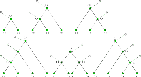
It is now clear that the velocity distribution $f_{k}$ can be drawn from the starting distribution $f_{0}$, choosing the different collisional trees with the same probability in mean. Off course two particles are produced in every collisional event, and only one of these is used to complete the collisional process. So it is natural to store the particle not used in a list, for its direct utilization in a future collisional process. In this way we can increase the efficiency of the method (if a particle sampled from a velocity density $f_{k}$ already exist it will not be necessary to obtain it by the complete collisional process) and guarantee the exact conservation of moments.

In order to do this we first split a set of $N$ particles into $m$ collision sets $N_{i}$, $i=0,\ldots,m$ where each set $N_{i}$ characterizes the number of particles that will undergo $i$ collisions in a time step $\Delta t$. All particles having more then $m$ collisions in the time step are thermalized (i.e. replaced with an equilibrium particle taken from the local Maxwellian), this number is denoted by $N_{m+1}$. Accordingly to this we have the following algorithm where $N$ and $m$ are given.

Algorithm 4.2 (Splitting particles into collision sets)

1.	set $\tau=1-\exp(-\mu\Delta t/\epsilon)$
	$n=0$, $\lambda_{0}=1$, $\omega_{0}=(1-\tau)$, $\tilde{N}_{0}=N$, $N_{c}=0$
	$N_{0}=\mathop{\mbox{\rm Iround}}\nolimits(\frac{\omega_{0}\tilde{N}_{0}}{\lambda_{0}})$
2.	repeat
		-	$n=n+1$,
		-	$\tilde{N}_{n}=\tilde{N}_{n-1}-N_{n-1}$
		-	$\omega_{n}=(1-\tau)\tau^{n}$
		-	$\lambda_{n}=\lambda_{n-1}-\omega_{n-1}$
		-	$N_{n}=\mathop{\mbox{\rm Iround}}\nolimits(\frac{\omega_{n}\tilde{N}_{n}}{\lambda_{n}})$
		-	$N_{c}=N_{c}+N_{n}$
	until $\tilde{N}_{n}>0$ and $n<m$
3.	if ($n=m$)
		-	$N_{m+1}=N-N_{c}-N_{0}$
	else
		-	$m=n$, $N_{m+1}=0$
	end if

Here, by $\mathop{\mbox{\rm Iround}}\nolimits(x)$, we denote a suitable integer rounding of a positive real number $x$. In our algorithm, we choose

$$\mathop{\mbox{\rm Iround}}\nolimits(x)=\left\{\begin{array}[]{lll}{[x]}&\mbox{with probability}&{[x]}+1-x,\\ {[x]}+1&\mbox{with probability}&x-{[x]},\end{array}\right.$$

where $[x]$ denotes the integer part of $x$.

Note that, since we have a finite number of particles, a consequence of the above splitting into collision sets is that the maximum possible length of a collision process is fixed by the initial number of particles $N$. The recursive collision algorithm for Maxwell molecules where thermalization occurs accordingly to a TR discretization of order $m$ is given here. To achieve exact conservation of momentum and energy and a better computational efficiency, the algorithm uses counters $c_{i}$ to keep track of the number of particles stored in memory with a collision history of $i$ collisions in a time step $\Delta t$ and not yet used in the simulation.

Algorithm 4.3 (TRMC-R for Maxwell molecules)

1.	compute the initial velocity of the particles, $\left\{v_{i}^{0},i=1,\ldots,N\right\}$
	by sampling them from the initial velocity $f_{0}$
2.	split particles into collision sets as in algorithm (4.2)
3.	set counters $c_{n}=0$ for $n=1,\ldots,m+1$
4.	for $n=m,\ldots,1$
		take $N_{n}$ samples from the distribution with density $f_{n}$, according to
		$\circ$	repeat
			-	choose $k\in\left\{0,1,\ldots,n-1\right\}$ with equal probability
			-	if $k=0$ take $v_{i}$ from the initial density $f_{0}$
			-	else choose $v_{i}$ from the density $f_{k}$
					if $c_{k}>0$ use a stored particle with a random choice
					set $c_{k}=c_{k}-1$ and $N_{k}=N_{k}+1$
					else sample $v_{i}$ and $v_{i}^{*}$ from $f_{k}$ (recursively)
					$v_{i}^{*}$ is stored and then set $c_{k}=c_{k}+1$, $N_{k}=N_{k}-1$
			-	if $n-k-1=0$ take $v_{j}$ from the initial density $f_{0}$
			-	else choose $v_{i}$ from the density $f_{n-k-1}$
					if $c_{n-k-1}>0$ use a stored particle with a random choice
					set $c_{n-k-1}=c_{n-k-1}-1$ and $N_{n-k-1}=N_{n-k-1}+1$
					else sample $v_{i}$ and $v_{i}^{*}$ from $f_{n-k-1}$ (recursively)
					$v_{i}^{*}$ is stored and then set $c_{n-k-1}=c_{n-k-1}+1$,
					$N_{n-k-1}=N_{n-k-1}-1$
			-	perform the collision between $v_{i}$ and $v_{j}$ as in DSMC
			-	$v^{\prime}_{i}$ and $v^{\prime}_{j}$ are random variables distributed
				according to the density $f_{n}$
			-	set $N_{n}=N_{n}-2$
			until $(N_{n}>0)$
	end for
5.	sample $N_{m+1}$ particles from the local Maxwellian

4.2 VHS collision kernels

The algorithm described for Maxwellian molecules can be extended to more general collision kernels by using dummy collisions and acceptance-rejection technique. This approach is equivalent to sample the post collisional velocity according to $P(f,f)/\mu$, where $\mu=4\pi{\bar{\sigma}}$ and ${\bar{\sigma}}$ is an upper bound of the scattering cross section for the given set of particles.

The upper bound ${\bar{\sigma}}$ should be chosen as small as possible, to avoid inefficient rejection, and it should be computed fast.

An optimal bound can be derived taking ${\bar{\sigma}}$ as

$${\bar{\sigma}}=\max_{v_{i},v_{j}}\sigma(|v_{i}-v_{j}|).$$ (28)

However this computation would be too expensive since it would require an $O(N^{2})$ operations. An upper bound of ${\bar{\sigma}}$ can be obtained by taking ${\bar{\sigma}}=\sigma(2\Delta v)$,

$$\Delta v=\max_{i}|v_{i}-\bar{v}|,\quad\bar{v}=\sum_{i}v_{i}/N.$$

In the VHS case the algorithm should be modified as follows

Algorithm 4.4 (TRMC-R for VHS molecules)

1.	compute the initial velocity of the particles, $\left\{v_{i}^{0},i=1,\ldots,N\right\}$
	by sampling them from the initial velocity $f_{0}$
2.	split particles into collision sets as in algorithm (4.2)
3.	set counters $c_{n}=0$ for $n=1,\ldots,m+1$
4.	compute an upper bound ${\bar{\sigma}}$ of $\sigma_{ij}=\sigma(v_{i},v_{j})$
5.	for $n=m,\ldots,1$
		take $N_{n}$ samples from the distribution with density $f_{n}$, according to
		point 4 of algorithm 4.3 where the dummy collision is performed as
		in DSMC if ${\bar{\sigma}}\xi_{1}<\sigma_{ij}$, with $\xi_{1}$ uniformly distributed random variable in ${[0,1]}$
6.	sample $N_{m+1}$ particles from the local Maxwellian

The algorithm is exactly conservative if combined with a suitable scheme for sampling a set of particles with prescribed momentum and energy from the Maxwellian, as proposed in [19] or by the authors in [17].

Remark 4.1

• In the case of $m=1,2$ the TRMC-R method corresponds to the first and second order TRMC methods presented in [16] for the simplest possible choice of the weights. Off course here we are aiming at using much larger values of $m\gg 1$ for which a direct extension of the algorithms presented in [16] is not feasible. Larger values of $m$ produce higher accurate results and then allow a larger time step when compared to [16, 17].

• Since the collision process changes the distribution function, it is important to choose a correct upper bound ${\bar{\sigma}}$ of $\sigma_{ij}$ in order to avoid discarding all the collisional trees computed in case $\sigma_{ij}>{\bar{\sigma}}$. As an alternative one can update the upper bound itself, after each collision as in [16, 17].

4.3 Adaptive technique for TRMC-R scheme

In practical simulations the number $m$ can be very large, depending on the Knudsen number and on the number of test particles. Clearly small values of $m$ make the algorithm faster, because the collision process is replaced by the projection to the local Maxwellian equilibrium, but far from the fluid regime keeping $m$ too small can produce less accurate results. In practice, a maximum allowed value $m_{\max}$ of $m$ is fixed at the beginning of the calculations; $m_{\max}$ represents the maximum depth of a collision tree. The main problem is to choose the right $m_{\max}$, in order to have the best combination between efficiency and accuracy. The idea we develop is to use an adaptive technique to choose the right maximum depths of the collision trees, based on evaluating the distance of the solution from the equilibrium through a suitable indicator. This can be performed measuring the variation of some macroscopic variables such as the fourth order moment or the components of the shear stress tensor.

Let $S$ be the macroscopic variable selected according to the particular physical problem. Then define the quantity

$$E_{1}=\frac{|{S^{n+1,m_{\max}}-S^{n}}|}{|{S^{n}}|}$$

that represents the relative variation at time step $n+1$ of the macroscopic variable $S$ computed with the solution obtained using $m_{\max}$ as maximum depth of the collision trees. If we fix an interval $\left[\delta_{1},\delta_{2}\right]$, $0<\delta_{1}<\delta_{2}$ then we can apply the following criteria in order to accept or discard the solution at time step $n+1$

• if $E_{1}<\delta_{1}$ the solution is accepted and $m_{\max}=m_{\max}/2$ in the next time step $n+2$;

• if $\delta_{1}\leq E_{1}\leq\delta_{2}$ the solution is accepted and $m_{\max}$ is unchanged in the next time step $n+2$;

• if $E_{1}>\delta_{2}$ the solution is discarded and the calculation is performed again using $m_{\max}=2m_{\max}$.

Off course it is possible to use other techniques in order to evaluate the distance from equilibrium [24].

The algorithm works with optimal efficiency if the collisions computed with the “wrong” $m_{\max}$ are kept and reused with $2m_{\max}$.

This can be done by starting with $m=m_{\min}$ and observing that if

$$\tilde{f}^{n+1,m}=\tau\sum_{k=0}^{m}(1-\tau)^{k}f_{k}+(1-\tau)^{m+1}M$$

then

$${f}^{n+1,2m}=\tilde{f}^{n+1,m}+\tau\sum_{k=m+1}^{2m}(1-\tau)^{k}f_{k}+[(1-\tau)^{2m+1}-(1-\tau)^{m+1}]M$$

So if the test for the adaptive strategy impose to discard the solution we proceed as follows

• the collisions computed with $m$ are kept;

• the fraction $(1-\tau)^{m+1}M$ is discarded;

• the fraction $\sum_{k=m+1}^{2m}(1-\tau)^{k}f_{k}$ is computed by the recursive collision process;

• the fraction $[(1-\tau)^{2m+1}-(1-\tau)^{m+1}]$ is sampled by a Maxwellian.

We observe that for estimation purposes the sampling from Maxwellian can be substitute by the analytical computation of local Maxwellian. This contributes to a better efficiency of the adaptive method.

Definition	left tree	right tree
(29)	7	7
(31)	3	2
(31)	3	43/16

Table 1: Length of the collision trees

4.4 Truncation of the collision trees for TRMC-R scheme

Off course several definitions of the length of trees are possible; the simplest one, that does not care about the shape of the collision trees that generate a particle from the density function $f_{k}$, is the one provided by

$$L(k=h+j+1)=k.$$ (29)

The length corresponds to the coefficient of the density function by which we sample the particle. The idea is to sample directly from the local Maxwellian if, for the collision process, $L(k)>m_{\max}$, $m_{\max}$ fixed, otherwise the whole tree is kept and the collisions are performed. This simple definition has been used into the algorithms described before. Different definition of length $L$ can be done using recursivity as

$$L(k=h+j+1) = 1+\min\{L(h),L(j)\},$$ (30)

$$L(k=h+j+1) = 1+\hbox{mean}\{L(h),L(j)\}.$$ (31)

These two last definitions can be related to the concept of “well balanced and not well balanced trees” (see Figure 2), i.e. if $L(k)>m_{\max}$ at the end of the collision process we can imagine that the particles would be more thermalized with respect to the ones that come from a tree where $L(k)<m_{\max}$. This off course is not true for definition (29).

In table (1) we show the values of the length of the collision trees reported in Figure (2) using the three different definitions.

The implementation of such strategy inside the recursive algorithm needs a modification of the first formulation given in section 4.2 because it is necessary to evaluate the length of collision trees without performing collisions. The idea is to write into a list the collision process (performed in a recursive way), to evaluate the length and to perform the collision using the collision process stored into the list.

The following algorithm shows how we can store the collision tree (correspondent to a process to sample from the density function $f_{k}$) into a list named $tree$ and how we can evaluate his length by using the recursive definition seen above.

Algorithm 4.5 (Storage and length of collision trees)

1.	assign to a variable $indx$ the value $indx=0$
2.	put $path(indx)=k$
3.	if	$k=0$ return $0$
	else	proceed as follows
		-	choose $j\in\left\{0,1,\ldots,k-1\right\}$ with equal probability
		-	put $h=k-j-1$
		-	increment the index: $indx=indx+1$
		-	store $j$ in the list: $path(indx)=j$
		-	increment the index: $indx=indx+1$
		-	store $h$ in the list: $path(indx)=h$
		-	return $(1+$
			$+\min\{($repeat from step 3 with $k=j),($repeat from step 3 with $k=h)\}$

In this way we obtain a list $path$ which contains the structure of the collision tree and its relative length using definition (31). Off course the same algorithm applies also to definition (31).

Figure 2: Well balanced (left) and not well balanced tree (right)

Now we can finally modify the algorithm 4.4 at the point 5 in order to use the previously created collision trees.

Algorithm 4.6 (TRMC-WB for VHS molecules)

1.	compute the initial velocity of the particles, $\left\{v_{i}^{0},i=1,\ldots,N\right\}$
	by sampling them from the initial velocity $f_{0}$
2.	split particles into collision sets as in algorithm (4.2)
3.	set counters $c_{n}=0$ for $n=1,\ldots,m+1$
4.	compute an upper bound ${\bar{\sigma}}$ of $\sigma_{ij}$
5.	for $n=m,\ldots,1$
		take $N_{n}$ samples from the distribution with density $f_{n}$, according to
		repeat
		-	compute the list $path$ and its length $L$ as in algorithm 4.5
		-	if $L>m_{\max}$
				set $N_{m+1}=N_{m+1}+1$ and $N_{n}=N_{n}-1$
			else
				set $indx=0,k=path(indx)$
			5.1.	if $k=0$ sample $v_{i}$ from the initial density $f_{0}$
				else	$indx=indx+1$
					set $j=path(indx)$
					set $indx=indx+1$
					set $h=path(indx)$
					if $c_{j}>0$	use a stored particle with a random choice
						set $c_{j}=c_{j}-1$, $N_{j}=N_{j}+1$ and $indx=indx+2j$
					else	sample $v_{i}$ and $v_{i}^{*}$ from $f_{j}$ (recursively from 5.1
						by setting $k=j$)
						$v_{i}^{*}$ is stored and then set $c_{j}=c_{j}+1$, $N_{j}=N_{j}-1$
					end if
					if $c_{h}>0$	use a stored particle with a random choice
						set $c_{h}=c_{h}-1$, $N_{h}=N_{h}+1$ and $indx=indx+2h$
					else	sample $v_{j}$ and $v_{j}^{*}$ from $f_{h}$ (recursively from 5.1
						by setting $k=h$)
						$v_{j}^{*}$ is stored and then set $c_{j}=c_{j}+1$, $N_{j}=N_{j}-1$
					end if
					Perform the dummy collision between $v_{i}$ and $v_{j}$ as in DSMC.
				end if
				set $N_{n}=N_{n}-2$
			end if
		until $(N_{n}>0)$
	end for
6.	sample $N_{m+1}$ particles from the local Maxwellian

Figure 3: Example of storage of a collision tree

Remark 4.2

In the Variable Hard Sphere case the calculation of algorithm 4.5 does not represent the effective length of the real collision trees, due to the dummy collisions which can occur during the total collision process. Thus the collisional trees performed in VHS model are usually longer than the ones for Maxwell molecules.

5 Numerical tests

We present some numerical tests, both in space homogeneous and space non homogeneous situations using the Hard Sphere model. The solution obtained by the Recursive Time Relaxed scheme combined with the adaptive strategy, is compared with the one obtained by the classic Bird’s algorithm.

To simplify notation we will use TRMC-R for the basic Recursive Time Relaxed Monte Carlo Scheme defined by Algorithm 4.4, TRMC-RAD for same scheme improved by the adaptivity strategy of section 4.3 (based on the shear stress tensor as equilibrium indicator) and TRMC-WB for the Recursive Time Relaxed Monte Carlo Scheme defined by Algorithm 4.6 (based on the well balanced truncation of the collision trees). With BIRD we refer to the classic DSMC scheme [3].

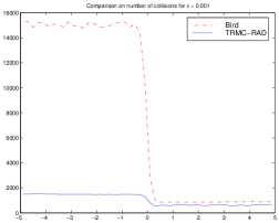
All macroscopic quantities have been considered in non dimensional form. As efficiency indicator we have considered the total number of collisions performed in the simulation. Sampling two particles from the Maxwellian has been counted as one collision. Note that due to the structure of the recursive algorithm in principle we may have additional computational requirements in terms of storage of particles during the evaluation of collision trees and storage and calculation of the collision trees if we want to implement a shape-depending truncation of the trees. However particle storage along the collision trees does not require any additional memory. In fact to achieve conservations each particle is used only one time in a collision tree and so it is the particle itself which is stored in the list. On the other hand the additional use of memory for the storage of the computational trees involves only one single collision history and thus the impact in the overall calculation is negligible.

5.1 Space homogeneous tests

We consider the sum of two Maxwellian as initial data. The solutions has been obtained in one single run using $5\times 10^{4}$ particles and choosing a collision time step $\Delta t/\epsilon$ equal to one. The reference solution, called in the plot as ”exact” has been obtained by a large number of averages on Bird’s scheme.

Figure 4: Evolution in Time of $4^{th}$ order moment (left) and relative error (right) for TRMC-R and Bird’s method.

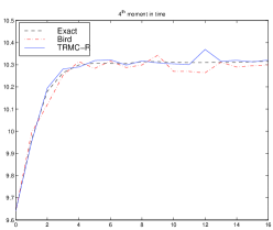
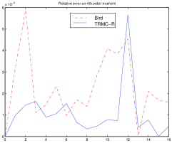
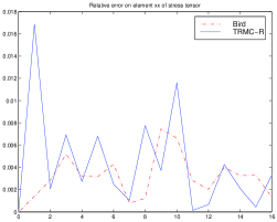
We compare the results for the fourth order moment $M_{4}$ and the component $P_{xx}$ of the shear stress tensor

$$M_{4}=\int_{\mathbb{R}^{3}}fv^{4}\,dv,\qquad P_{xx}=\int_{\mathbb{R}^{3}}f(v_{1}-u_{1})^{2}\,dv.$$

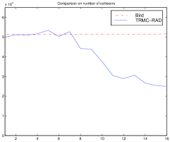
Figure 4 shows the case of TRMC-R without any limit for the maximum depth of collision trees. The agreement with respect to Bird’s scheme is very good, and if we look at the relative errors we can observe that they are comparable. In Figure 5 we plot the relative error for the shear stress tensor component $P_{xx}$ and the number of collisions necessary to perform the simulations. We can consider the number of collisions as an index of efficiency in terms of computational time. A single sample from a Maxwellian is counted as half of a collision. As expected we had no gain in efficiency because with this scheme we took into account all possible collision processes.

Figure 5: Relative error for the evolution in time of the stress tensor component $P_{xx}$ (left) and number of collisions (right) for TRMC-R and Bird’s method.

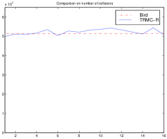
In the next case (Figure 6 and 7) we perform the same simulation using TRMC-RAD, starting with $m_{max}=2$ and taking $\delta_{1}=0.005$ and $\delta_{2}=0.01$. We preserve accuracy with respect to DSCM solution, but we have obtained a strong reduction of the computational time because a bigger fraction of particles is sampled directly from the Maxwellian without going through the whole collision tree.

Figure 6: Evolution in Time of $4^{th}$ order moment (left) and relative error (right) for TRMC-RAD and Bird’s method.

Figure 7: Relative error for the evolution in time of the stress tensor component $P_{xx}$ (left) and number of collisions (right) for TRMC-RAD and Bird’s method.

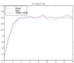
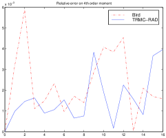
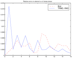
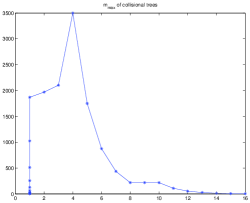
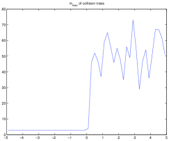
We observe in Figure 8, where we report the maximum depth of the collision trees during the calculation, that the simulation in the first time steps has been performed several times, using at each time $m_{\max}=2m_{\max}$. As already mentioned let us point out that these calculations do not affect the total computational cost because all “old collisions” are kept and reused in order to complete the new collision process.

Figure 8: Maximum depth $m_{max}$ of a collision tree in time for TRMC-RAD

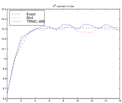
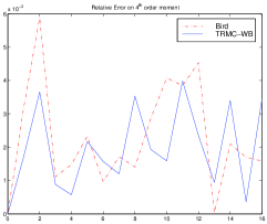
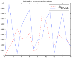
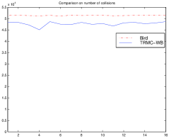
The last homogeneous test deals with the shape depending strategy based on truncation of collision trees by using the definition $L(k=h+j+1)=1+\min\{L(h),L(j)\}$ and $m_{\max}=5$. Similar results can be obtained using the definition $L(k=h+j+1)=1+{\rm mean}\{L(h),L(j)\}$, we omit them for brevity. We have, also in this case, a gain in efficiency, preserving the accuracy in time (see Figures 9 and 10).

The TRMC-WB scheme shows a constant gain of computational cost with respect to Bird’s scheme, approximatively the 7% during the whole simulation, while the TRMC-RAD achieves the maximum gain (about 50%) at the end of the calculation, with an average gain of 20% in the total simulation time. The combination of TRMC-WB and TRMC-RAD is under investigation and will be presented elsewhere.

Figure 9: Evolution in Time of $4^{th}$ order moment (left) and relative error (right) for TRMC-WB and Bird’s method.

Figure 10: Relative error for the evolution in time of stress tensor component $P_{xx}$ (left) and number of collisions (right) for TRMC-WB and Bird’s method.

5.2 Stationary shock

Next we consider a non homogeneous stationary shock problem. The boundary conditions have been assigned at the left and right side accordingly to the Rankine-Hugoniot relations

$$\rho_{L}u_{L}=\rho_{R}u_{R},$$

$$\rho_{L}u_{L}^{2}+p_{L}=\rho_{R}u_{R}^{2}+p_{R},$$

$$u_{L}(E_{L}+p_{L})=u_{R}(E_{R}+p_{R}).$$

The values used in the simulation are

• $M_{a_{L}}=3$ (Mach Number of incoming flux)

• $T_{L}=1$ (Temperature of incoming flux)

• $u_{x_{L}}=-M\sqrt{\gamma T_{L}},\,u_{y_{L}}=0,\,u_{z_{L}}=0$ $\gamma=5/3$ (Mean velocity of incoming flux)

• $\rho_{L}=1$ (Total mass)

• $\epsilon=1$, $\epsilon=0.1$ and $\epsilon=0.001$.

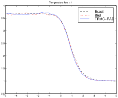
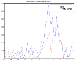
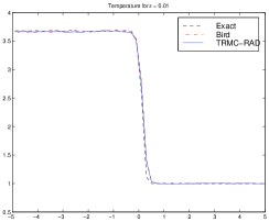
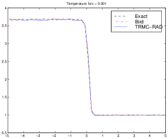
The numerical solution has been obtained using TRMC-RAD and Bird’s method with $50$ spatial cells and $1000$ particles in each cell. Reference ’Exact’ solution has been performed by Bird’s standard DSMC method using $50$ spatial cells and $3000$ particles in each cell. A detailed analysis on the effect of the number of particles per cell in TRMC methods has been performed in [21, 22].

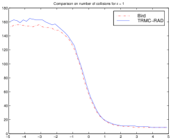
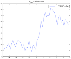
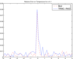
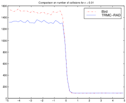
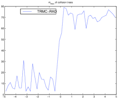
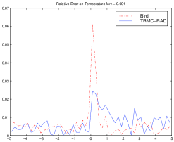
In order to increase accuracy, for $t$ large enough, averages of the solution have been computed. The results for the temperature shock are presented in Figures 11-16. As expected there is a good agreement between TRMC-RAD and Bird’s method and the relative errors are essentially comparable.

Note that there is an evident gain in efficiency of TRMC-RAD against Bird’s method without losing accuracy, especially near fluid regime. Looking at the rarefied case $\epsilon=1$ we obtain the same computational cost, while we have a gain close to 10% for the intermediate test case $\epsilon=0.1$ that increases up to the 86% close to the fluid regime for $\epsilon=0.001$.

6 Conclusion

We have presented recursive Monte Carlo methods which are suitable for the numerical simulation of the Boltzmann equation for a wide range of Knudsen numbers. These recursive TRMC methods minimize the effects of time discretization error and over-relaxation due to the choice of the upper bound of the cross-section that were present in the previous versions of TRMC. Of paramount importance to increase the efficiency of the methods is the use of suitable truncation strategies of the collisional trees, such as adaptive truncation based on macroscopic quantities or well balanced truncation based on the trees properties. The resulting schemes are very promising and show that a considerable gain in efficiency can be obtained without degradation in accuracy. However additional test cases must be performed in order to validate the schemes. A combination of the present schemes with the hybrid strategy proposed in [15] is actually under investigation.

Figure 11: Rarefied regime ($\epsilon=1$). Temperature (left) and Relative Error (right) for TRMC-RAD and Bird’s method.

Figure 12: Rarefied regime ($\epsilon=1$). Number of collisions for TRMC-RAD and Bird’s method (left) and maximum depth $m_{\max}$ in each cell for TRMC-RAD (right).

Figure 13: Intermediate regime ($\epsilon=0.1$). Temperature (left) and Relative Error (right) for TRMC-RAD and Bird’s method.

Figure 14: Intermediate regime ($\epsilon=0.1$). Number of collisions for TRMC-RAD and Bird’s method (left) and maximum depth $m_{\max}$ in each cell for TRMC-RAD (right).

Figure 15: Fluid regime ($\epsilon=0.001$). Temperature (left) and Relative Error (right) for TRMC-RAD and Bird’s method.

Figure 16: Fluid regime ($\epsilon=0.001$). Number of collisions for TRMC-RAD and Bird’s method (left) and maximum depth $m_{\max}$ in each cell for TRMC-RAD (right).

References

- [1] H. Babovsky, On a simulation scheme for the Boltzmann equation, Math. Methods Appl. Sci., 8 (1986), pp. 223–233.
- [2] L.L. Baker, N.G. Hadjiconstantinou, Variance Reduction for Monte Carlo Solutions of the Boltzmann Equation Phys. of Fluids, 17, 051703, 1 4, (2005).
- [3] G. A. Bird, Molecular gas dynamics and the direct simulation of gas flows, Oxford University Press, USA (1994).
- [4] J. F. Bourgat, P. LeTallec, B. Perthame, and Y. Qiu, Coupling Boltzmann and Euler equations without overlapping, in Domain Decomposition Methods in Science and Engineering, Contemp. Math. 157, AMS, Providence, RI, (1994), pp. 377–398.
- [5] I. D. Boyd, Q. Sun, A direct simulation method for subsonic, microscale gas flows, J. Comp. Phys., 179, 2, (2002) pp. 400–425.
- [6] E. A. Carlen, M. C. Carvalho, and E. Gabetta, Central limit theorem for Maxwellian molecules and truncation of the Wild expansion, Comm. Pure Appl. Math., 53 (2000), pp. 370–397.
- [7] C. Cercignani, The Boltzmann Equation and Its Applications, Springer-Verlag, New York, 1988.
- [8] E. Gabetta, L. Pareschi, and G. Toscani, Relaxation schemes for nonlinear kinetic equations, SIAM J. Numer. Anal., 34 (1997), pp. 2168–2194.
- [9] A.L. Garcia, J.B. Bell, W.Y. Crutchfield and B.J. Alder, Adaptive mesh and algorithm refinement using Direct Simulation Monte Carlo J. Comp. Phys., 154, 134-55, (1999).
- [10] D.B. Hash and H.A. Hassan, Assessment of schemes for coupling Monte Carlo and Navier-Stokes solution methods J. Thermophys. Heat Transf., 10, 242-249, (1996).
- [11] T.M.M. Homolle and N.G. Hadjiconstantinou, Low-variance Deviational Simulation Monte Carlo Phys. of Fluids, 19, 041701, (2007).
- [12] Z.-H. Li and H.-X. Zhang, Numerical investigation from rarefied flow to continuum by solving the Boltzmann model equation Int. J. Num. Meth. Fluids Volume, 42, 4, 361–382, (2003).
- [13] M. Kac, Probability and Related Topics in Physical Sciences, Lectures in Appl. Math., Interscience Publishers, London, New York, 1959.
- [14] K. Nanbu, Direct simulation scheme derived from the Boltzmann equation, J. Phys. Soc. Japan, 49 (1980), pp. 2042–2049.
- [15] L. Pareschi and R. E. Caflisch, Implicit Monte Carlo methods for rarefied gas dynamics I: The space homogeneous case, J. Comput. Phys., 154 (1999), pp. 90–116.
- [16] L. Pareschi and G. Russo, Time Relaxed Monte Carlo methods for the Boltzmann equation, SIAM J. Sci. Comput. 23 (2001), pp. 1253–1273.
- [17] L. Pareschi, S. Trazzi, Numerical solution of the Boltzmann equation by Time Relaxed Monte Carlo (TRMC) methods, Int. J. Num. Meth. Fluids, 48 (2005); pp. 947-983.
- [18] L. Pareschi and B. Wennberg, A recursive Monte Carlo method for the Boltzmann equation in the Maxwellian case, Monte Carlo Methods Appl., 7 (2001), pp. 349–358.
- [19] D. I. Pullin, Direct simulation methods for compressible inviscid ideal gas flow, J. Comput. Phys., 34 (1980), pp. 231–244.
- [20] D. I. Pullin, Generation of normal variates with given sample, J. Statist. Comput. Simulation, 9 (1979), pp. 303–309.
- [21] G.Russo, L.Pareschi, S.Trazzi, A.Shevyrin, Ye. Bondar, M.IvanovComparison between Time Relaxed Monte Carlo Method and Majorant Frequency Scheme methods for the space homogeneous Boltzmann equation, AIP American Institute of Physics - Conference proceedings, 768 (2005); pp. 577-588.
- [22] G.Russo, L.Pareschi, S.Trazzi, A.Shevyrin, Ye. Bondar, M.IvanovPlane Couette Flow Computations by TRMC and MFS Methods, AIP American Institute of Physics - Conference proceedings, 768 (2005); pp. 583-588.
- [23] T.E. Schwartzentruber and I.D. Boyd, A Hybrid Particle-Continuum Method Applied to Shock Waves, J. Comp. Phys., Vol. 215, 2006, pp. 402-416.
- [24] S.Tiwari, S. RjasanowSobolev norm as a criterion of local thermal equilibrium, Eur. J. Mech. B/Fluids, Vol.16 n.6 (1997).
- [25] C. Truesdell and R. G. Muncaster, Fundamentals of Maxwell Kinetic Theory of a Simple Monatomic Gas, Academic Press, New York, 1980.
- [26] E. Wild, On Boltzmann’s equation in the kinetic theory of gases, Proc. Cambridge Philos. Soc., 47 (1951), pp. 602–609.