Implicit-explicit Runge-Kutta schemes and applications to hyperbolic systems with relaxation

Abstract

We consider new implicit-explicit (IMEX) Runge-Kutta methods for hyperbolic systems of conservation laws with stiff relaxation terms. The explicit part is treated by a strong-stability-preserving (SSP) scheme, and the implicit part is treated by an L-stable diagonally implicit Runge-Kutta methods (DIRK). The schemes proposed are asymptotic preserving (AP) in the zero relaxation limit. High accuracy in space is obtained by Weighted Essentially Non Oscillatory (WENO) reconstruction. After a description of the mathematical properties of the schemes, several applications will be presented.

Keywords : Runge-Kutta methods, hyperbolic systems with relaxation, stiff systems, high order shock capturing schemes.

AMS Subject Classification : 65C20, 82D25

1 Introduction

Several physical phenomena of great importance for applications are described by stiff systems of differential equations in the form

$$\partial_{t}U={\cal F}(U)+\frac{1}{\varepsilon}R(U),$$ (1)

where $U=U(t)\in{\mathbb{R}}^{N}$, ${\cal F},R:{\mathbb{R}}^{N}\to{\mathbb{R}}^{N}$ and $\varepsilon>0$ is the stiffness parameter.

System (1) may represent a system of $N$ ODE’s or a discretization of a system of PDE’s, such as, for example, convection-diffusion equations, reaction-diffusion equations and hyperbolic systems with relaxation.

In this work we consider the latter case, which in recent years has been a very active field of research, due to its great impact on applied sciences [13, 31]. For example, we mention that hyperbolic systems with relaxation appears in kinetic theory of rarefied gases, hydrodynamical models for semiconductors, viscoelasticity, multiphase flows and phase transitions, radiation hydrodynamics, traffic flows, shallow waters, etc.

In one space dimension these systems have the form

$$\partial_{t}U+\partial_{x}F(U)=\frac{1}{{\varepsilon}}R(U),\quad x\in{\mathbb{R}},$$ (2)

that corresponds to (1) for ${\cal F}(U)=-\partial_{x}F(U)$. In (2) the Jacobian matrix $F^{\prime}(U)$ has real eigenvalues and admits a basis of eigenvectors $\forall\,U\in{\mathbb{R}}^{N}$ and ${\varepsilon}$ is called relaxation parameter.

The development of efficient numerical schemes for such systems is challenging, since in many applications the relaxation time varies from values of order one to very small values if compared to the time scale determined by the characteristic speeds of the system. In this second case the hyperbolic system with relaxation is said to be stiff and typically its solutions are well approximated by solutions of a suitable reduced set of conservation laws called equilibrium system [13].

Usually it is extremely difficult, if not impossible, to split the problem in separate regimes and to use different solvers in the stiff and non stiff regions. Thus one has to use the original relaxation system in the whole computational domain. The construction of schemes that work for all ranges of the relaxation time, using coarse grids that do not resolve the small relaxation time, has been studied mainly in the context of upwind methods using a method of lines approach combined with suitable operator splitting techniques [10, 26] and more recently in the context of central schemes [30, 35].

Splitting methods have been widely used for such problems. They are attractive because of their simplicity and robustness. Strang splitting provides second order accuracy if each step is at least second order accurate [45]. This property is maintained under fairly mild assumptions even for stiff problems [24]. However, Strang splitting applied to hyperbolic systems with relaxation reduces to first order accuracy when the problem becomes stiff. The reason is that the kernel of the relaxation operator is non trivial, which corresponds to a singular matrix in the linear case, and therefore the assumptions in [24] are not satisfied.

Furthermore with a splitting strategy it is difficult to obtain higher order accuracy even in non stiff regimes (high order splitting schemes can be constructed, see [16], but they are seldom used because of stability problems).

Recently developed Runge-Kutta schemes overcome this difficulties, providing basically the same advantages of the splitting schemes, without the drawback of the order restriction [10, 26, 49].

In this paper we will present some recent results on the development of high order, underresolved Runge-Kutta time discretization for such systems. In particular, using the formalism of implicit-explicit (IMEX) Runge-Kutta schemes [4, 5, 36, 11, 49] we derive new IMEX schemes up to order 3 that are strong-stability-preserving (SSP) for the limiting system of conservation laws (such methods were originally referred to as total variation diminishing (TVD) methods, see [18, 19, 44]).

To this aim, we derive general conditions that guarantee the asymptotic preserving property, i.e. the consistency of the scheme with the equilibrium system and the asymptotic accuracy, i.e. the order of accuracy is maintained in the stiff limit. For a stability analysis of IMEX schemes we refer to [38].

The rest of the paper is organized as follows. In Section 2 we introduce the general structure of IMEX Runge-Kutta schemes. Section 3 is devoted to IMEX Runge-Kutta schemes applied to hyperbolic systems with relaxation. In Section 4 we describe space discretization obtained by conservative finite-volume and finite difference schemes. In Section 5 we present some numerical results concerning the accuracy of IMEX schemes when applied to a prototype hyperbolic system with relaxation. Finally in Section 6 we investigate the performance of the schemes in several realistic applications to shallow waters, traffic flows and granular gases.

2 IMEX Runge-Kutta schemes

An IMEX Runge-Kutta scheme consists of applying an implicit discretization to the source terms and an explicit one to the non stiff term. When applied to system (1) it takes the form

$$U^{(i)} = U^{n}-{\Delta t}\sum_{j=1}^{i-1}\tilde{a}_{ij}\partial_{x}F(U^{(j)})+{\Delta t}\sum_{j=1}^{\nu}a_{ij}\frac{1}{\varepsilon}R(U^{(j)}),$$ (3)

$$U^{n+1} = U^{n}-{\Delta t}\sum_{i=1}^{\nu}\tilde{w}_{i}\partial_{x}F(U^{(i)})+{\Delta t}\sum_{i=1}^{\nu}w_{i}\frac{1}{\varepsilon}R(U^{(i)}).$$ (4)

The matrices $\tilde{A}=(\tilde{a}_{ij})$, $\tilde{a}_{ij}=0$ for $j\geq i$ and $A=(a_{ij})$ are $\nu\times\nu$ matrices such that the resulting scheme is explicit in $F$, and implicit in $R$. An IMEX Runge-Kutta scheme is characterized by these two matrices and the coefficient vectors $\tilde{w}=(\tilde{w}_{1},\ldots,\tilde{w}_{\nu})^{T}$, $w=(w_{1},\ldots,w_{\nu})^{T}$.

Since the simplicity and efficiency of solving the algebraic equations corresponding to the implicit part of the discretization at each step is of paramount importance, it is natural to consider diagonally implicit Runge-Kutta (DIRK) schemes [22] for the source terms ($a_{ij}=0$, for $j>i$).

IMEX Runge-Kutta schemes can be represented by a double tableau in the usual Butcher notation,

$$\begin{array}[]{c|c}\tilde{c}&\tilde{A}\\ \hline\cr\\ &\tilde{w}^{T}\end{array}\qquad\qquad\begin{array}[]{c|c}c&A\\ \hline\cr\\ &w^{T}\end{array}$$

where the coefficients $\tilde{c}$ and $c$ used for the treatment of non autonomous systems, are given by the usual relation

$$\tilde{c}_{i}=\sum_{j=1}^{i-1}\tilde{a}_{ij},\quad c_{i}=\sum_{j=1}^{i}a_{ij}.$$ (5)

The use of a DIRK scheme for $R$ is a sufficient condition to guarantee that $F$ is always evaluated explicitly.

In the case of system (2), in order to obtain a numerical scheme, a suitable space discretization of equations (3)-(4) is required. This discretization can be performed at the level of the original system (2) in which case one has a system of ODEs that is then solved in time by the IMEX scheme (method of lines). Alternatively one can apply a suitable space discretization directly to the time discrete equations (3)-(4).

Finally we remark that previously developed schemes, such as the Additive semi-implicit Runge-Kutta methods of Zhong [49], and the splitting Runge-Kutta methods of Jin et al. [26], [10] can be rewritten as IMEX-RK schemes [38].

2.1 Order conditions

The general technique to derive order conditions for Runge-Kutta schemes is based on the Taylor expansion of the exact and numerical solution.

In particular, conditions for schemes of order $p$ are obtained by imposing that the solution of system (2) at time $t=t_{0}+\Delta t$, with a given initial condition at time $t_{0}$, agrees with the numerical solution obtained by one step of a Runge-Kutta scheme with the same initial condition, up to order ${\Delta t}^{p+1}$.

Here we report the order conditions for IMEX Runge-Kutta schemes up to order $p=3$, which is already considered high order for PDEs problems.

We apply scheme (3)-(4) to system (2), with $\varepsilon=1$. We assume that the coefficients $\tilde{c}_{i}$, $c_{i}$, $\tilde{a}_{ij}$, $a_{ij}$ satisfy conditions (5). Then the order conditions are the following

First order

$$\sum_{i=1}^{\nu}\tilde{w}_{i}=1,\quad\sum_{i=1}^{\nu}w_{i}=1.$$ (6)

Second order

$$\sum_{i}\tilde{w}_{i}\tilde{c}_{i}=1/2,\quad\sum_{i}w_{i}c_{i}=1/2,$$ (7)

$$\sum_{i}\tilde{w}_{i}c_{i}=1/2,\quad\sum_{i}w_{i}\tilde{c}_{i}=1/2.$$ (8)

Third order

$$\sum_{ij}\tilde{w}_{i}\tilde{a}_{ij}\tilde{c}_{j}=1/6,\quad\sum_{i}\tilde{w}_{i}\tilde{c}_{i}\tilde{c}_{i}=1/3,\quad\sum_{ij}w_{i}a_{ij}c_{j}=1/6,\quad\sum_{i}w_{i}c_{i}c_{i}=1/3,$$ (9)

$$\begin{array}[]{c}\sum_{ij}\tilde{w}_{i}\tilde{a}_{ij}c_{j}=1/6,\quad\sum_{ij}\tilde{w}_{i}a_{ij}\tilde{c}_{j}=1/6,\quad\sum_{ij}\tilde{w}_{i}a_{ij}c_{j}=1/6,\\[14.45377pt] \sum_{ij}w_{i}\tilde{a}_{ij}c_{j}=1/6,\quad\sum_{ij}w_{i}a_{ij}\tilde{c}_{j}=1/6,\quad\sum_{ij}w_{i}\tilde{a}_{ij}\tilde{c}_{j}=1/6,\\[14.45377pt] \sum_{i}\tilde{w}_{i}c_{i}c_{i}=1/3,\quad\sum_{i}\tilde{w}_{i}\tilde{c}_{i}c_{i}=1/3,\quad\sum_{i}w_{i}\tilde{c}_{i}\tilde{c}_{i}=1/3,\quad\sum_{i}w_{i}\tilde{c}_{i}c_{i}=1/3.\end{array}$$ (13)

Conditions (6), (7), (9) are the standard order conditions for the two tableau, each of them taken separately. Conditions (8) and (13) are new conditions that arise because of the coupling of the two schemes.

The order conditions will simplify a lot if $\tilde{c}=c$. For this reason only such schemes are considered in [4]. In particular, we observe that, if the two tableau differ only for the value of the matrices $A$, i.e. if $\tilde{c}_{i}=c_{i}$ and $\tilde{w}_{i}=w_{i}$, then the standard order conditions for the two schemes are enough to ensure that the combined scheme is third order. Note, however, that this is true only for schemes up to third order.

Higher order conditions can be derived as well using a generalization of Butcher 1-trees to 2-trees, see [11]. However the number of coupling conditions increase dramatically with the order of the schemes. The relation between coupling conditions and accuracy of the schemes is reported in Table 1.

IMEX-RK	Number of coupling conditions
order	General case	$\tilde{w}_{i}=w_{i}$	$\tilde{c}=c$	$\tilde{c}=c$ and $\tilde{w}_{i}=w_{i}$
1	0	0	0	0
2	2	0	0	0
3	12	3	2	0
4	56	21	12	2
5	252	110	54	15
6	1128	528	218	78

Table 1: Number of coupling conditions in IMEX Runge-Kutta schemes

3 Applications to hyperbolic systems with relaxation

In this section we give sufficient conditions for asymptotic preserving and asymptotic accuracy properties of IMEX schemes. This properties are strongly related to L-stability of the implicit part of the scheme.

3.1 Zero relaxation limit

Let us consider here one-dimensional hyperbolic systems with relaxation of the form (2). The operator $R:{\mathbb{R}}^{N}\to{\mathbb{R}}^{N}$ is called a relaxation operator, and consequently (2) defines a relaxation system, if there exists a constant $n\times N$ matrix $Q$ with rank$(Q)=n<N$ such that

$$QR(U)=0\quad\forall\,\,U\in{\mathbb{R}}^{N}.$$ (14)

This gives $n$ independent conserved quantities $u=QU$. Moreover we assume that equation $R(U)=0$ can be uniquely solved in terms of $u$, i.e.

$$U={\cal E}(u)\,\,\,\hbox{such that}\,\,\,R({\cal E}(u))=0.$$ (15)

The image of ${\cal E}$ represents the manifold of local equilibria of the relaxation operator $R$.

Using (14) in (2) we obtain a system of $n$ conservation laws which is satisfied by every solution of (2)

$$\partial_{t}(QU)+\partial_{x}(QF(U))=0.$$ (16)

For vanishingly small values of the relaxation parameter ${\varepsilon}$ from (2) we get $R(U)=0$ which by (15) implies $U={\cal E}(u)$. In this case system (2) is well approximated by the equilibrium system [13].

$$\partial_{t}u+\partial_{x}G(u)=0,$$ (17)

where $G(u)=QF({\cal E}(u))$.

System (17) is the formal limit of system (1) as ${\varepsilon}\to 0$. The solution $u(x,t)$ of the system will be the limit of $QU$, with $U$ solution of system (1), provided a suitable condition on the characteristic velocities of systems (1) and (17) is satisfied (the so called subcharacteristic condition, see [48, 13].)

3.2 Asymptotic properties of IMEX schemes

We start with the following

Definition 3.1

We say that an IMEX scheme for system (2) in the form (3)-(4) is asymptotic preserving (AP) if in the limit $\varepsilon\to 0$ the scheme becomes a consistent discretization of the limit equation (17).

Note that this definition does not imply that the scheme preserves the order of accuracy in $t$ in the stiff limit $\epsilon\to 0$. In the latter case the scheme is said asymptotically accurate.

In order to give sufficient conditions for the AP and asymptotically accurate property, we make use of the following simple

Lemma 3.1

If all diagonal elements of the triangular coefficient matrix $A$ that characterize the DIRK scheme are non zero, then

$$\lim_{\epsilon\to 0}R(U^{(i)})=0.$$ (18)

Proof:
In the limit $\epsilon\to 0$ from (3) we have

$$\sum_{j=1}^{i}a_{ij}R(U^{j})=0,\quad i=1,\ldots,\nu.$$

Since the matrix $A$ is non-singular, this implies $R(U^{i})=0,\>i=1,\ldots,\nu$.

 

In order to apply the previous lemma, the vectors of $c$ and $\tilde{c}$ cannot be equal. In fact $\tilde{c}_{1}=0$ whereas $c_{1}\neq 0$. Note that if $c_{1}=0$ but $a_{ii}\neq 0$ for $i>1$, then we still have $\lim_{\epsilon\to 0}R(U^{(i)})=0$ for $i>1$ but $\lim_{\epsilon\to 0}R(U^{(1)})\neq 0$ in general. The corresponding scheme may be inaccurate if the initial condition is not “well prepared” ($R(U_{0})\neq 0$). In this case the scheme is not able to treat the so called “initial layer” problem and degradation of accuracy in the stiff limit is expected (see Section 5 and references [10, 36, 35].) On the other hand, if the initial condition is “well prepared” ($R(U^{(0)})=0$), then relation (18), $i=1,\ldots,\nu$ holds even if $a_{11}=c_{1}=0$.

Next we can state the following

Theorem 3.1

If $\det A\neq 0$ in the limit $\epsilon\to 0$, the IMEX scheme (3)-(4) applied to system (2) becomes the explicit RK scheme characterized by $(\tilde{A},\tilde{w},\tilde{c})$ applied to the limit equation (17).

Proof:
As in the case of the continuous system, multiplying equations (3) and (4) by the matrix $Q$, and making use of the relation $QR(U)=0\>\forall\,U$, we obtain

$$u^{(i)}=u_{0}+h\sum_{j=1}^{i-1}\tilde{a}_{ij}QF(U^{(j)}),$$ (19)

and

$$u_{1}=u_{0}+h\sum_{i=1}^{\nu}\tilde{w}_{i}QF(U^{(i)}),$$ (20)

where

$$u^{(i)}=QU^{(i)},\>i=1,\ldots\nu,\quad u_{0}=QU_{0},\quad u_{1}=QU_{1}.$$

From the previous lemma, in the stiff limit one has

$$R(U^{(i)})=0,\>i=1,\ldots\nu,$$

and, from property (15) of the relaxation operator $R$, this implies

$$U^{(i)}={\cal E}(u^{(i)}),\>i=1,\ldots\nu.$$

Substituting this expression in (19)-(20) one obtains

$$u^{(i)}=u_{0}+h\sum_{j=1}^{i-1}\tilde{a}_{ij}G(u^{(j)}),$$ (21)

and

$$u_{1}=u_{0}+h\sum_{i=1}^{\nu}\tilde{w}_{i}G(u^{(i)}),$$ (22)

where $G(u)=QF({\cal E}(u))$.

 

Clearly one may claim that if the implicit part of the IMEX scheme is A-stable or L-stable the previous theorem is satisfied. Note however that this is true only if the tableau of the implicit integrator does not contain any column of zeros that makes it reducible to a simpler A-stable or L-stable form. Some remarks are in order.

Remarks:

• There is a close analogy between hyperbolic systems with stiff relaxation and differential algebraic equations (DAE) [3]. The limit system as $\epsilon\to 0$ is the analog of an index 1 DAE, in which the algebraic equation is explicitly solved in terms of the differential variable. In the context of DAE, the initial condition that we called “well prepared” is called “consistent”.

• This result does not guarantee the accuracy of the solution for the $N-n$ non conserved quantities. In fact, since the very last step in the scheme is not a projection towards the local equilibrium, a final layer effect occurs. The use of stiffly accurate schemes (i.e. schemes for which $a_{\nu j}=w_{j},j=1,\ldots,\nu$) in the implicit step may serve as a remedy to this problem.

• The theorem guarantees that in the stiff limit the numerical scheme becomes the explicit RK scheme applied to the equilibrium system, and therefore the order of accuracy of the limiting scheme is greater or equal to the order of accuracy of the original IMEX scheme.

When constructing numerical schemes for conservation laws, one has to take a great care in order to avoid spurious numerical oscillations arising near discontinuities of the solution. This is avoided by a suitable choice of space discretization (see Section 4) and time discretization.

Solution of scalar conservation equations, and equations with a dissipative source have some norm that decreases in time. It would be desirable that such property is maintained at a discrete level by the numerical method. If $U^{n}$ represents a vector of solution values (for example obtained from a method of lines approach in solving (17)) we recall the following [44]

Definition 3.2

A sequence $\{U^{n}\}$ is said to be strongly stable in a given norm $||\cdot||$ provided that $||U^{n+1}||\leq||U^{n}||$ for all $n\geq 0$.

The most commonly used norms are the $TV$-norm and the infinity norm. A numerical scheme that maintains strong stability at discrete level is called Strong Stability Preserving (SSP).

Here we review some basic facts about RK-SSP schemes. First, it has been shown [19] under fairly general conditions that high order SSP schemes are necessarily explicit. Second, observe that a generic explicit RK scheme can be written as

$$U^{(0)} = U^{n}$$

$$U^{(i)} = \sum_{k=0}^{i-1}(\alpha_{ik}U^{(k)}+{\Delta t}\beta_{ik}L(U^{(k)}),\quad i=1,\ldots,\nu,$$ (23)

$$U^{n+1} = U^{(\nu)}$$

where $\alpha_{ik}\geq 0$ and $\alpha_{ik}=0$ only if $\beta_{ik}=0$. This representation of RK schemes (which is not unique) can be converted to a standard Butcher form in a straightforward manner. Observe that for consistency, one has $\sum_{k=0}^{i-1}\alpha_{ik}=1$. It follows that if the scheme can be written in the form (23) with non negative coefficients $\beta_{ik}$ then it is a convex combination of Forward Euler steps, with step sizes $\beta_{ik}/\alpha_{ik}{\Delta t}$. A consequence of this is that if Forward Euler is SSP for ${\Delta t}\leq{\Delta t}^{*}$, then the RK scheme is also SSP for ${\Delta t}\leq c{\Delta t}^{*}$, with $c=\min_{ik}(\alpha_{ik}/\beta_{ik})$ [40, 19].

The constant $c$ is a measure of the efficiency of the SSP-RK scheme, therefore for the applications it is important to have $c$ as large as possible. For a detailed description of optimal SSP schemes and their properties see [44].

By point iii) of the above remarks it follows that if the explicit part of the IMEX scheme is SSP then, in the stiff limit, we will obtain an SSP method for the limiting conservation law. This property is essential to avoid spurious oscillations in the limit scheme for equation (17).

In this section we give the Butcher tableau for the new second and third order IMEX schemes that satisfy the conditions of Theorem 3.1. In all these schemes the implicit tableau corresponds to an L-stable scheme, that is $w^{T}A^{-1}e=1$, $e$ being a vector whose components are all equal to 1 [22], whereas the explicit tableau is SSP$k$, where $k$ denotes the order of the SSP scheme. Several examples of asymptotically SSP schemes are reported in tables (2)-(6). We shall use the notation SSP$k$$(s,\sigma,p)$, where the triplet $(s,\sigma,p)$ characterizes the number $s$ of stages of the implicit scheme, the number $\sigma$ of stages of the explicit scheme and the order $p$ of the IMEX scheme.

$$\begin{array}[]{c|cc}0&0&0\\ 1&1&0\\ \hline\cr&1/2&1/2\end{array}\qquad\begin{array}[]{c|cccc}\gamma&\gamma&0\\ 1-\gamma&1-2\gamma&\gamma\\ \hline\cr&1/2&1/2\end{array}\qquad\gamma=1-\frac{1}{\sqrt{2}}$$

Table 2: Tableau for the explicit (left) implicit (right) IMEX-SSP2(2,2,2) L-stable scheme

$$\begin{array}[]{c|ccc}0&0&0&0\\ 0&0&0&0\\ 1&0&1&0\\ \hline\cr&0&1/2&1/2\end{array}\qquad\begin{array}[]{c|cccc}1/2&1/2&0&0\\ 0&-1/2&1/2&0\\ 1&0&1/2&1/2\\ \hline\cr&0&1/2&1/2\end{array}$$

Table 3: Tableau for the explicit (left) implicit (right) IMEX-SSP2(3,2,2) stiffly accurate scheme

$$\begin{array}[]{c|ccc}0&0&0&0\\ 1/2&1/2&0&0\\ 1&1/2&1/2&0\\ \hline\cr&1/3&1/3&1/3\end{array}\qquad\begin{array}[]{c|cccc}1/4&1/4&0&0\\ 1/4&0&1/4&0\\ 1&1/3&1/3&1/3\\ \hline\cr&1/3&1/3&1/3\end{array}$$

Table 4: Tableau for the explicit (left) implicit (right) IMEX-SSP2(3,3,2) stiffly accurate scheme

$$\begin{array}[]{c|ccc}0&0&0&0\\ 1&1&0&0\\ 1/2&1/4&1/4&0\\ \hline\cr&1/6&1/6&2/3\end{array}\qquad\begin{array}[]{c|ccc}\gamma&\gamma&0&0\\ 1-\gamma&1-2\gamma&\gamma&0\\ 1/2&1/2-\gamma&0&\gamma\\ \hline\cr&1/6&1/6&2/3\end{array}\qquad\gamma=1-\frac{1}{\sqrt{2}}$$

Table 5: Tableau for the explicit (left) implicit (right) IMEX-SSP3(3,3,2) L-stable scheme

$$\begin{array}[]{c|cccc}0&0&0&0&0\\ 0&0&0&0&0\\ 1&0&1&0&0\\ 1/2&0&1/4&1/4&0\\ \hline\cr&0&1/6&1/6&2/3\end{array}\qquad\begin{array}[]{c|cccc}\alpha&\alpha&0&0&0\\ 0&-\alpha&\alpha&0&0\\ 1&0&1-\alpha&\alpha&0\\ 1/2&\beta&\eta&1/2-\beta-\eta-\alpha&\alpha\\ \hline\cr&0&1/6&1/6&2/3\end{array}$$

$$\alpha=0.24169426078821,\quad\beta=0.06042356519705\quad\eta=0.12915286960590$$

Table 6: Tableau for the explicit (left) implicit (right) IMEX-SSP3(4,3,3) L-stable scheme

4 IMEX-WENO schemes

For simplicity we consider the case of the single scalar equation

$$u_{t}+f(u)_{x}=\frac{1}{{\varepsilon}}{r}(u).$$ (24)

We have to distinguish between schemes based on cell averages (finite volume approach, widely used for conservation laws) and schemes based on point values (finite difference approach).

Let ${\Delta x}$ and $\Delta t$ be the mesh widths. We introduce the grid points

$$x_{j}=j{\Delta x},\quad x_{j+1/2}=x_{j}+\frac{1}{2}{{\Delta x}},\quad j=\ldots,-2,-1,0,1,2,\ldots$$

and use the standard notations

$$u_{j}^{n}=u(x_{j},t^{n}),\qquad\bar{u}_{j}^{n}=\frac{1}{{\Delta x}}\int_{x_{j-1/2}}^{x_{j+1/2}}u(x,t^{n})\,dx.$$

4.1 Finite volumes

Integrating equation (24) on $I_{j}=[x_{j-1/2},x_{j+1/2}]$ and dividing by $\Delta x$ we obtain

$$\frac{d\bar{u}_{j}}{dt}=-\frac{1}{{\Delta x}}[f(u(x_{j+1/2},t))-f(u(x_{j-1/2},t))]+\frac{1}{{\varepsilon}}\overline{r(u)}_{j}.$$ (25)

In order to convert this expression into a numerical scheme, one has to approximate the right hand side with a function of the cell averages $\{\bar{u}(t)\}_{j}$, which are the basic unknowns of the problem.

The first step is to perform a reconstruction of the unknown function $u(x,t)$ by a piecewise polynomial, starting from cell averages $\bar{u}_{j}(t)$. Given $\{\bar{u}_{j}\}$, compute a piecewise polynomial reconstruction

$${\cal R}(x)=\sum_{j}P_{j}(x)\chi_{j}(x),$$

where $P_{j}(x)$ is a polynomial satisfying some accuracy and non oscillatory property, and $\chi_{j}(x)$ is the indicator function of cell $I_{j}$. For first order schemes, the reconstruction is piecewise constant, while second order schemes can be obtained by a piecewise linear reconstruction. Higher order schemes are obtained by higher order polynomials.

The reconstruction step is very delicate, because the function $u(x,t)$ may be discontinuous. To this goal, suitable techniques, such as Weighted Essentially Non Oscillatory (WENO), have been developed. The reader can consult the review by Shu [41] and references therein for a more detailed description of high order non oscillatory reconstructions.

The flux function at the edge of the cell can be computed by using a suitable numerical flux function, consistent with the analytical flux,

$$f(u(x_{j+1/2},t))\approx F(u_{j+1/2}^{-},u_{j+1/2}^{+}),$$

where the quantities $u_{j+1/2}^{\pm}$ are obtained from the reconstruction, as $u_{j+1/2}^{\pm}=\lim_{x\to x_{j+1/2}^{\pm}}{\cal R}(x)$.

Example of numerical flux functions are the Godunov flux

$$F(u_{j+1/2}^{-},u_{j+1/2}^{+})=f(u^{*}(u_{j+1/2}^{-},u_{j+1/2}^{+})),$$

where $u^{*}(u_{j+1/2}^{-},u_{j+1/2}^{+})$ is the solution of the Riemann problem at $x_{j+1/2}$, corresponding to the states $u_{j+1/2}^{-}$ and $u_{j+1/2}^{+}$, and the Local Lax Friedrichs flux (also known as Rusanov flux),

$$F(u_{j+1/2}^{-},u_{j+1/2}^{+})=\frac{1}{2}[(f(u_{j+1/2}^{-})+f(u_{j+1/2}^{+}))-\alpha(u_{j+1/2}^{+}-u_{j+1/2}^{-})],$$

where $\alpha=\max_{w}|f^{\prime}(w)|$, and the maximum is taken over the relevant range of $w$.

The two examples constitute two extreme cases of numerical fluxes: the Godunov flux is the most accurate and the one that produces the best results for a given grid size, but it is very expensive, since it requires the solution to the Riemann problem. Local Lax-Friedrichs flux, on the other hand, is less accurate, but much cheaper. This latter is the numerical flux that has been used throughout all the calculations performed for this paper. The difference in resolution provided by the various numerical fluxes becomes less relevant with the increase in the order of accuracy of the method.

The right hand side of Eq.(25) contains the average of the source term $\overline{r(u)}$ instead of the source term evaluated at the average of $u$, $r(\bar{u})$. The two quantities agree within second order accuracy

$$\overline{r(u)}_{j}=r(\bar{u}_{j})+O({\Delta x}^{2}).$$

This approximation can be used to construct schemes up to second order.

First order (in space) semidiscrete schemes can be obtained using the numerical flux function $F(\bar{u}_{j},\bar{u}_{j+1})$ in place of $f(u(x_{j+1/2},t))$,

$$\frac{d\bar{u}_{j}}{dt}=-\frac{F(\bar{u}_{j},\bar{u}_{j+1})-F(\bar{u}_{j-1},\bar{u}_{j})}{{\Delta x}}+\frac{1}{{\varepsilon}}{r(\bar{u}_{j})}.$$ (26)

Second order schemes are obtained by using a piecewise linear reconstruction in each cell, and evaluating the numerical flux on the two sides of the interface

$$\frac{d\bar{u}}{dt}=-\frac{F(u_{j+1/2}^{-},u_{j+1/2}^{+})-F(u_{j-1/2}^{-},u_{j-1/2}^{+})}{{\Delta x}}+\frac{1}{{\varepsilon}}r(\bar{u}_{j})$$

The quantities at cell edges are computed by piecewise linear reconstruction. For example,

$$u_{j+1/2}^{-}=\bar{u}_{j}+\frac{{\Delta x}}{2}u^{\prime}_{j}$$

where the slope $u^{\prime}_{j}$ is a first order approximation of the space derivative of $u(x,t)$, and can be computed by suitable slope limiters (see, for example, [29] for a discussion on TVD slope limiters.)

For schemes of order higher than second, a suitable quadrature formula is required to approximate $\overline{g(u)}_{j}$. For example, for third and fourth order schemes, one can use Simpson’s rule

$$\overline{r(u)}_{j}\approx\frac{1}{6}(r(u_{j-1/2}^{+})+4r(u_{j})+r(u_{j+1/2}^{-}))$$

where the pointwise values $u_{j-1/2}^{+}$, $u_{j}$, $u_{j+1/2}^{-}$ are obtained from the reconstruction.

For a general problem, this has the effect that the source term couples the cell averages of different cells, thus making almost impractical the use of finite volume methods for high order schemes applied to stiff sources.

Note, however, that in many relevant cases of hyperbolic systems with relaxation the implicit step, thanks to the conservation properties of the system, can be explicitly solved, and finite volume methods can be successfully used. We mention here all relaxation approximation of Jin-Xin type [28], some simple discrete velocity models, such as Carlemann and Broadwell models, monoatomic gas in Extended Thermodynamics, semiconductor models, and shallow water equations.

4.2 Finite differences

In a finite difference scheme the basic unknown is the pointwise value of the function, rather than its cell average. Osher and Shu observed that it is possible to write a finite difference scheme in conservative form [42]. Let us consider the equation

$$\frac{\partial u}{\partial t}+\frac{\partial f}{\partial x}=\frac{1}{{\varepsilon}}r(u),$$

and write

$$\frac{\partial f}{\partial x}(u(x,t))=\frac{\hat{f}(u(x+\frac{{\Delta x}}{2},t))-\hat{f}(u(x-\frac{{\Delta x}}{2},t))}{{\Delta x}}.$$

The relation between $f$ and $\hat{f}$ is the following. Let us consider the sliding average operator

$$\bar{u}(x,t)=<u>_{x}\equiv\frac{1}{{\Delta x}}\int_{x-\frac{{\Delta x}}{2}}^{x+\frac{{\Delta x}}{2}}{u(\xi,t)\,d\xi}.$$

Differentiating with respect to $x$ one has

$$\frac{\partial\bar{u}}{\partial x}=\frac{1}{{\Delta x}}(u(x+\frac{{\Delta x}}{2},t)-u(x-\frac{{\Delta x}}{2},t)).$$

Therefore the relation between $f$ and $\hat{f}$ is the same that exists between $\bar{u}(x,t)$ and $u(x,t)$, namely, flux function $f$ is the cell average of the function $\hat{f}$. This also suggests a way to compute the flux function. The technique that is used to compute pointwise values of $u(x,t)$ at the edge of the cell from cell averages of $u$ can be used to compute $\hat{f}(u(x_{j+1/2},t))$ from $f(u(x_{j},t))$. This means that in the finite difference method it is the flux function which is computed at $x_{j}$ and then reconstructed at $x_{j+1/2}$. But the reconstruction at $x_{j+1/2}$ may be discontinuous. Which value should one use? A general answer to this question can be given if one considers flux functions that can be split

$$f(u)=f^{+}(u)+f^{-}(u)\hskip 1.0pt,$$ (27)

with the condition that

$$\frac{df^{+}(u)}{du}\geq 0\hskip 1.0pt,\quad\frac{df^{-}(u)}{du}\leq 0.$$ (28)

There is a close analogy between flux splitting and numerical flux functions. In fact, if a flux can be split as  (27), then

$$F(a,b)=f^{+}(a)+f^{-}(b)$$

will define a monotone consistent flux, provided condition (28) is satisfied. Together with non oscillatory reconstructions (such as WENO) and SSP time discretization, the monotonicity condition will ensure that the overall scheme will not produce spurious numerical oscillations (see, for example, [29, 41].)

This is the case, for example, of the local Lax-Friedrichs flux. A finite difference scheme therefore takes the following form

$$\frac{du_{j}}{dt}=-\frac{1}{{\Delta x}}[\hat{F}_{j+1/2}-\hat{F}_{j-1/2}]+\frac{1}{{\varepsilon}}g(u_{j}),$$

$$\hat{F}_{j+1/2}=\hat{f}^{+}(u_{j+1/2}^{-})+\hat{f}^{-}(u_{j+1/2}^{+});$$

$\hat{f}^{+}(u_{j+1/2}^{-})$ is obtained by

• computing $f^{+}(u_{l})$ and interpret it as cell average of $\hat{f}^{+}$;

• performing pointwise reconstruction of $\hat{f}^{+}$ in cell $j$, and evaluate it in $x_{j+1/2}$.

$\hat{f}^{-}(u_{j+1/2}^{+})$ is obtained by

• computing $f^{-}(u_{l})$, interpret as cell average of $\hat{f}^{-}$;

• performing pointwise reconstruction of $\hat{f}^{-}$ in cell $j+1$, and evaluate it in $x_{j+1/2}$.

A detailed account on high order finite difference schemes can be found in [41].

At variance with finite volume schemes, since the source is evaluated pointwise, finite difference schemes do not couple the cells. This is a big advantage in the cases in which the implicit step can not be explicitly solved.

Remarks:

• Finite difference can be used only with uniform (or smoothly varying) mesh. In this respect finite volume are more flexible, since they can be used even with unstructured grids.

• The treatment presented for the scalar equation can be extended to systems, with a minor change of notation. In particular, the parameter $\alpha$ appearing in the local Lax-Friedrichs flux will be computed using the spectral radius of the Jacobian matrix.

• For schemes applied to systems, better results are usually obtained if one uses characteristic variables rather than conservative variables in the reconstruction step. The use of conservative variables may result in the appearance of small spurious oscillations in the numerical solution. For a treatment of this effect see, for example, [39].

5 Numerical tests

In this section we investigate numerically the convergence rate and the zero relaxation limit behavior of the schemes. To this aim we apply the IMEX-WENO schemes to the Broadwell equations of rarefied gas dynamics [10, 26, 30, 35]. In all the computations presented in this paper we used finite difference WENO schemes with Lax-Friedrichs flux and conservative variables. Of course the sharpness of the resolution of the numerical results can be improved using a less dissipative flux.

As a comparison, together with the new IMEX-SSP schemes, we have considered the second order ARS(2,2,2) method presented in [4], which was the one recommended by the authors. For this scheme, since $c_{1}=0$, there will be a degradation of accuracy due to the initial layer.

In all figures, the value of $N$ represents the number of grid points in space.

The kinetic model is characterized by a hyperbolic system with relaxation of the form (2) with

$$U=(\rho,\,m,\,z),\qquad F(U)=(m,\,z,\,m),\qquad R(U)=\left(0,\,0,\,\frac{1}{2}{(\rho^{2}+m^{2}-2\rho z)}\right).$$

Here ${\varepsilon}$ represents the mean free path of particles. The only conserved quantities are the density $\rho$ and the momentum $m$.

In the fluid-dynamic limit ${\varepsilon}\to 0$ we have

$$z=z_{E}\equiv\frac{\rho^{2}+m^{2}}{2\rho},$$ (29)

and the Broadwell system is well approximated by the reduced system (17) with

$$u=(\rho,\,\rho v),\qquad G(u)=\left(\rho v,\,\frac{1}{2}(\rho+\rho v^{2})\right),\qquad v=\frac{m}{\rho},$$

which represents the corresponding Euler equations of fluid-dynamics.

Convergence rates

We have considered a periodic smooth solution with initial data as in [10, 30] given by

$$\rho(x,0)=1+a_{\rho}\sin\frac{2\pi x}{L},\quad v(x,0)=\frac{1}{2}+a_{v}\sin\frac{2\pi x}{L},\quad z(x,0)=a_{z}\frac{\rho(x,0)^{2}+m(x,0)^{2}}{2\rho(x,0)}.$$ (30)

In our computations we used the parameters

$$a_{\rho}=0.3,\quad a_{v}=0.1,\quad a_{z}=1.0\mbox{ (no initial layer) and }a_{z}=0.2\mbox{ (initial layer)},\quad L=20,$$ (31)

and we integrate the equations for $t\in[0,30]$. A Courant number $\Delta t/\Delta x=0.6$ has been used. The plots of the relative error are given in Figure 1.

Figure 1: Relative errors for density $\rho$ in the Broadwell equations with initial data (31). Left column $a_{z}=1.0$ (no initial layer), right column $a_{z}=0.2$ (initial layer). From top to bottom, ${\varepsilon}=1.0,\,10^{-3},\,10^{-6}$.

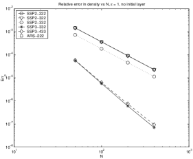
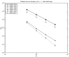
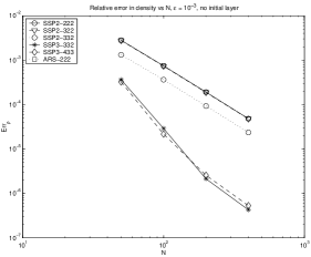
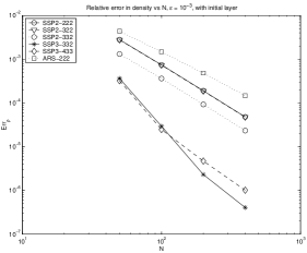
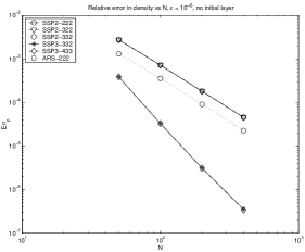
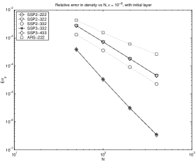
Notice how, in absence of initial an layer, all schemes tested have the prescribed order of accuracy both in the non stiff and in the stiff limit, with some degradation of the accuracy at intermediate regimes. As expected, scheme ARS(2,2,2), shows a degradation of the accuracy when an initial layer is present.

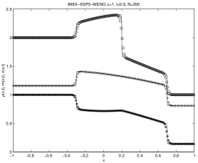
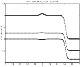
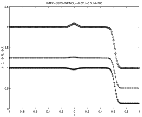
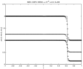
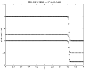
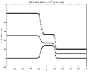
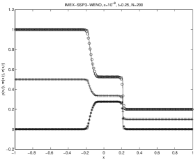
Next we test the shock capturing properties of the schemes in the case of non smooth solutions characterized by the following two Riemann problems [10]

$$\rho_{l}=2,\qquad m_{l}=1,\qquad\qquad\quad z_{l}=1,\qquad x < 0.2,$$

$$\rho_{r}=1,\qquad m_{r}=0.13962,\qquad z_{r}=1,\qquad x > 0.2,$$

$$\rho_{l}=1,\quad\qquad m_{l}=0,\qquad z_{l}=1,\qquad x < 0,$$

$$\rho_{r}=0.2,\qquad m_{r}=0,\qquad z_{r}=1,\qquad x > 0.$$

For brevity we report the numerical results obtained with the second order IMEX-SSP2(2,2,2) and third order IMEX-SSP3(4,3,3) schemes that we will refer to as IMEX-SSP2-WENO and IMEX-SSP3-WENO respectively. The result are shown in Figures 2 and 3 for a Courant number $\Delta t/\Delta x=0.5$. Both schemes, as expected, give an accurate description of the solution in all different regimes also using coarse meshes that do not resolve the small scales. In particular the shock formation in the fluid limit is well captured without spurious oscillations. We refer to [10, 26, 30, 35, 2] for a comparison of the present results with previous ones.

Figure 2: Numerical solution of the Broadwell equations with initial data (5) for $\rho$($\circ$), $m$($\ast$) and $z$($+$) at time $t=0.5$. Left column IMEX-SSP2-WENO scheme, right column IMEX-SSP3-WENO scheme. From top to bottom, ${\varepsilon}=1.0,\,0.02,\,10^{-8}$.

Figure 3: Numerical solution of the Broadwell equations with initial data (5) for $\rho$($\circ$), $m$($\ast$) and $z$($+$) at time $t=0.25$ for ${\varepsilon}=10^{-8}$. Left IMEX-SSP2-WENO scheme, right IMEX-SSP3-WENO scheme.

6 Applications

Finally we present some numerical results obtained with IMEX-SSP2-WENO and IMEX-SSP3-WENO concerning situations in which hyperbolic systems with relaxation play a major role in applications. The results have been obtained with $N=200$ grid points. As usual the reference solution is computed on a much finer grid.

6.1 Shallow water

First we consider a simple model of shallow water flow [26]

$$\partial_{t}h+\partial_{x}(hv) = 0,$$

$$\partial_{t}(hv)+\partial_{x}(h+\frac{1}{2}h^{2}) = \frac{h}{\epsilon}(\frac{h}{2}-v),$$

where $h$ is the water height with respect to the bottom and $hv$ the flux.

The zero relaxation limit of this model is given by the inviscid Burgers equation.

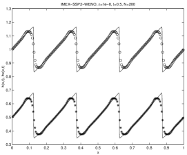
The initial data we have considered is [26]

$$h=1+0.2\sin(8\pi x),\quad hv=\frac{h^{2}}{2},$$

with $x\in[0,1]$. The solution at $t=0.5$ in the stiff regime $\epsilon=10^{-8}$ using periodic boundary conditions is given in Figure 4. For IMEX-SSP2-WENO the dissipative effect due to the use of the Lax-Friedrichs flux is very pronounced. As expected this effect becomes less relevant with the increase of the order of accuracy. We refer to [26] for a comparison with the present results.

Figure 4: Numerical solution of the shallow water model with initial data (6.1) for $h$($\circ$) and $hv$($\ast$) at time $t=0.5$ for ${\varepsilon}=10^{-8}$. Left IMEX-SSP2-WENO scheme, right IMEX-SSP3-WENO scheme.

6.2 Traffic flows

In [6] a new macroscopic model of vehicular traffic has been presented. The model consists of a continuity equation for the density $\rho$ of vehicles together with an additional velocity equation that describes the mass flux variations due to the road conditions in front of the driver. The model can be written in conservative form as follows

$$\partial_{t}\rho+\partial_{x}(\rho v) = 0,$$

$$\partial_{t}(\rho w)+\partial_{x}(v\rho w) = A\frac{\rho}{T}(V(\rho)-v),$$

where $w=v+P(\rho)$ with $P(\rho)$ a given function describing the anticipation of road conditions in front of the drivers and $V(\rho)$ describes the dependence of the velocity with respect to the density for an equilibrium situation. The parameter $T$ is the relaxation time and $A>0$ is a positive constant.

If the relaxation time goes to zero, under the subcharacteristic condition

$$-P^{\prime}(\rho)\leq V^{\prime}(\rho)\leq 0,\quad\rho>0,$$

we obtain the Lighthill-Whitham [48] model

$$\partial_{t}\rho+\partial_{x}(\rho V(\rho))=0.$$ (36)

A typical choice for the function $P(\rho)$ is given by

$$P(\rho)=\left\{\begin{array}[]{cc}\frac{c_{v}}{\gamma}\left(\frac{\rho}{\rho_{m}}\right)^{\gamma}&\gamma>0,\\ {c_{v}}\ln\left(\frac{\rho}{\rho_{m}}\right)&\gamma=0,\end{array}\right.$$

where $\rho_{m}$ is a given maximal density and $c_{v}$ a constant with dimension of velocity.

In our numerical results we assume $A=1$ and an equilibrium velocity $V(\rho)$ fitting to experimental data [7]

$$V(\rho)=v_{m}\frac{\pi/2+\arctan\left(\alpha\frac{\rho/\rho_{m}-\beta}{\rho/\rho_{m}-1}\right)}{\pi/2+\arctan\left(\alpha\beta\right)}$$

with $\alpha=11$, $\beta=0.22$ and $v_{m}$ a maximal speed. We consider $\gamma=0$ and, in order to fulfill the subcharacteristic condition, assume $c_{v}=2$. All quantities are normalized so that $v_{m}=1$ and $\rho_{m}=1$.

We consider a Riemann problem centered at $x=0$ with left and right states

$$\rho_{L}=0.05,\quad v_{L}=0.05,\qquad\rho_{R}=0.05,\quad v_{R}=0.5.$$ (37)

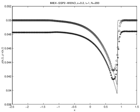
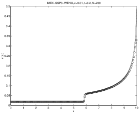
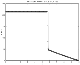
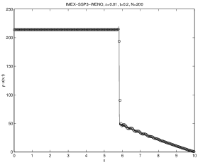
The solution at $t=1$ for $T=0.2$ is given in Figure 5. The figure shows the development of the density of the vehicles. Both schemes gives very similar results. Again, in the second order scheme the shock is smeared out if compared to the third order case. See [7] for more numerical results.

Figure 5: Numerical solution of the traffic model with initial data (37) for $\rho$($\circ$) and $\rho v$($\ast$) at time $t=1$ for ${\varepsilon}=0.2$. Left IMEX-SSP2-WENO scheme, right IMEX-SSP3-WENO scheme.

6.3 Granular gases

We consider the continuum equations of Euler type for a granular gas [25, 47]. These equations have ben derived for a dense gas composed of inelastic hard spheres. The model reads

$$\rho_{t}+(\rho u)_{x} = 0,$$

$$(\rho u)_{t}+(\rho u^{2}+p)_{x} = \rho g,$$

$$\left(\frac{1}{2}\rho u^{2}+\frac{3}{2}\rho T\right)_{t}+\left(\frac{1}{2}\rho u^{3}+\frac{3}{2}u\rho T+pu\right)_{x} = -\frac{(1-e^{2})}{\epsilon}G(\rho){\rho^{2}T^{3/2}},$$

where $e$ is the coefficient of restitution, $g$ the acceleration due to gravity, $\epsilon$ a relaxation time, $p$ is the pressure given by

$$p=\rho T(1+2(1+e)G(\rho)),$$

and $G(\rho)$ is the statistical correlation function. In our experiments we assume

$$G(\rho)=\nu\left(1-\left(\frac{\nu}{\nu_{M}}\right)^{\frac{4}{3}\nu_{M}}\right)^{-1},$$

where $\nu=\sigma^{3}\rho\pi/6$ is the volume fraction, $\sigma$ is the diameter of a particle, and $\nu_{M}=0.64994$ is 3D random close-packed constant.

We consider the following initial data [32] on the interval $[0,10]$

$$\rho=34.37746770,\quad v=18,\quad P=1589.2685472,$$ (39)

which corresponds to a supersonic flow at Mach number $M_{a}=7$ (the ratio of the mean fluid speed to the speed of sound). Zero-flux boundary condition have been used on the bottom (right) boundary whereas on the top (left) we have an ingoing flow characterized by (39).

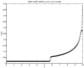
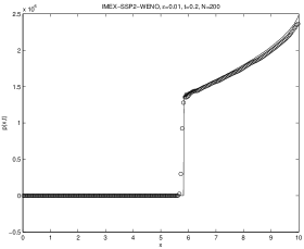
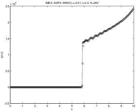
The values of the restitution coefficient and the particle diameter have been taken $e=0.97$ and $\sigma=0.1$. We report the solution at $t=0.2$ with $\epsilon=0.01$ in Figure 6 (see [32] for similar results). Due to the nonlinearity of the source term the implicit solver has been efficiently solved using Newton’s method in each cell thanks to the use of finite difference space discretization.

Both methods provide a good description of the shock that propagates backward after the particles impact with the bottom. Note that the second order method provides excessive smearing of the layer at the right boundary. This problem is not present in the third order scheme. However due to the use of conservative variables we can observe the presence of small spurious oscillations in the pressure profile.

Figure 6: Numerical solution of the hydrodynamical model of a granular gas with initial data (39). Left column IMEX-SSP2-WENO scheme, right column IMEX-SSP3-WENO scheme. From top to bottom, mass fraction $\nu$, velocity $\rho u$ and pressure $p$.

References

- [1] G. Akridis, M. Crouzeix, C. Makridakis, Implicit-explicit multistep methods for quasilinear parabolic equations, Numer. Math. 82 (1999), no. 4, pp. 521–541.
- [2] M. Arora, P.L. Roe, Issues and strategies for hyperbolic problems with stiff source terms in Barriers and challenges in computational fluid dynamics, Hampton, VA, 1996, Kluwer Acad. Publ., Dordrecht, (1998), pp. 139–154.
- [3] U. Ascher,, L. Petzold, Computer Methods for Ordinary Differential Equations, and Differential Algebraic Equations, SIAM, Philadelphia, (1998).
- [4] U. Ascher, S. Ruuth, R. J. Spiteri, Implicit-explicit Runge-Kutta methods for time dependent Partial Differential Equations, Appl. Numer. Math. 25, (1997), pp. 151–167.
- [5] U. Ascher, S. Ruuth, B. Wetton, Implicit-explicit methods for time dependent PDE’s, SIAM J. Numer. Anal., 32, (1995), pp. 797–823.
- [6] A. Aw, M. Rascle, Resurrection of second order models of traffic flow ?, SIAM. J. Appl. Math. 60, (2000), pp. 916–938.
- [7] A. Aw, A. Klar, T. Materne, M. Rascle, Derivation of continuum traffic flow models from microscopic follow the leader models, SIAM J. Appl. Math. 63, (2002), pp. 259–278.
- [8] J. Butcher, The numerical analysis of Ordinary differential equations. Runge-Kutta and general linear methods.. John Wiley & Sons, Chichester and New York (1987).
- [9] M. Briani, R. Natalini, G. Russo, Implicit–Explicit numerical schemes for jump diffusion processes, in preparation (2004).
- [10] R. E. Caflisch, S. Jin, G. Russo, Uniformly accurate schemes for hyperbolic systems with relaxation, SIAM J. Numer. Anal., 34, (1997), pp. 246–281.
- [11] C. A. Kennedy, M. H. Carpenter, Additive Runge-Kutta schemes for convection-diffusion-reaction equations, Appl. Numer. Math. 44 (2003), 139–181.
- [12] M. Cecchi Morandi, M. Redivo-Zaglia, G. Russo, Extrapolation methods for hyperbolic systems with relaxation, Journal of Computational and Applied Mathematics 66 (1996), pp. 359–375.
- [13] G. Q. Chen, D. Levermore, T. P. Liu, Hyperbolic conservations laws with stiff relaxation terms and entropy, Comm. Pure Appl. Math., 47, (1994), pp. 787–830.
- [14] K. Dekker, J. G. Verwer, Stability of Runge-Kutta Methods for Stiff Nonlinear Differential Equations, North-Holland, Amsterdam (1984).
- [15] B. O. Dia, M. Schatzman, Estimation sur la formule de Strang, C. R. Acad. Sci. Paris, t.320, Série I (1995), pp. 775–779.
- [16] B. O. Dia, M. Schatzman, Commutateur de certains semi-groupes holomorphes et applications aux directions alternées, Mathematical Modelling and Numerical Analysis 30 (1996), pp. 343–383.
- [17] J. Frank, W. H. Hundsdorfer, J. G. Verwer, On the stability of implicit-explicit linear multistep methods, Special issue on time integration (Amsterdam, 1996). Appl. Numer. Math. 25 (1997), no. 2-3, 193–205.
- [18] S. Gottlieb, C. -W. Shu, Total Variation Diminishing Runge-Kutta schemes, Math. Comp. 67 (1998), pp. 73–85.
- [19] S. Gottlieb, C. -W. Shu, E. Tadmor, Strong-stability-preserving high order time discretization methods, SIAM Review, 43 (2001), pp. 89–112.
- [20] E. Hairer, Order conditions for numerical methods for Partitioned ordinary differential equations, Numerische Mathematik 36 (1981) pp. 431-445.
- [21] E. Hairer, S. P. Nørsett, G. Wanner, Solving ordinary differential equations, Vol.1 Nonstiff problems, Springer-Verlag, New York (1987).
- [22] E. Hairer, G. Wanner, Solving ordinary differential equations, Vol.2 Stiff and differential-algebraic problems, Springer-Verlag, New York (1987).
- [23] E. Hofer A partially implicit method for large stiff systems of Ode’s with only few equations introducing small time-constants, SIAM J. Numer. Anal. 13, (1976) pp. 645-663.
- [24] T. Jahnke, C. Lubich, Error bounds for exponential operator splitting, BIT, (2000), pp. 735–744.
- [25] J. Jenkins, M. Richman, Grad’s 13-moment system for a dense gas of inelastic spheres, Arch. Rat. Mechanics, 87, (1985), pp. 355–377.
- [26] S. Jin, Runge-Kutta methods for hyperbolic systems with stiff relaxation terms J. Comput. Phys., 122 (1995), pp. 51–67.
- [27] S. Jin, C. D. Levermore, Numerical Schemes for hyperbolic conservation laws with stiff relaxation terms, J. Comp. Physics, 126 (1996), pp. 449–467.
- [28] S. Jin, Z.P. Xin, The relaxation schemes for systems of conservation laws in arbitrary space dimensions, Comm. Pure Appl. Math. 48 (1995), no. 3, 235–276.
- [29] R. J. LeVeque, Numerical Methods for Conservation Laws, Lectures in Mathematics, Birkhauser Verlag, Basel (1992).
- [30] S. F. Liotta, V. Romano, G. Russo, Central schemes for balance laws of relaxation type, SIAM J. Numer. Anal., 38, (2000), pp. 1337–1356.
- [31] T. P. Liu, Hyperbolic conservation laws with relaxation, Comm. Math. Phys., 108, (1987), pp. 153–175.
- [32] A. Marquina, S. Serna, Capturing shock waves in inelastic granular gases, UCLA-CAM Report, 04-04 february (2004).
- [33] M. L. Minion, Semi-implicit spectral deferred correction methods for ordinary differential equations, Comm. Math. Sciences, 1, No.3, p. 471–500.
- [34] I. Müller, T. Ruggeri, Rational extended thermodynamics, Springer-Verlag, Berlin, (1998).
- [35] L. Pareschi, Central differencing based numerical schemes for hyperbolic conservation laws with stiff relaxation terms, SIAM J. Num. Anal., 39, (2001), pp. 1395-1417.
- [36] L. Pareschi, G. Russo, Implicit-explicit Runge-Kutta schemes for stiff systems of differential equations, Advances Theo. Comp. Math., 3, (2000), pp. 269–289.
- [37] L. Pareschi, G. Russo, High order asymptotically strong-stability-preserving methods for hyperbolic systems with stiff relaxation, Proceedings HYP2002, Pasadena USA, Springer (2003), pp. 241–255.
- [38] L. Pareschi, G. Russo, Stability analysis of Implicit-Explicit Runge-Kutta schemes, preprint (2004).
- [39] Jianxian Qiu, Chi-Wang Shu, On the construction, comparison, and local characteristic decomposition for high-order central WENO schemes, J. Comput. Phys. 183 (2002), no. 1, 187–209
- [40] C. -W. Shu, Total variation diminishing time discretizations, SIAM J. Sci. Stat. Comput., 9, (1988), 1073–1084.
- [41] C. -W. Shu, Essentially Non Oscillatory and Weighted Essentially NOn OScillatory Schemes for Hyperbolic Conservation Laws, in Advanced numerical approximation of nonlinear hyperbolic equations, Lecture Notes in Mathematics, 1697, (2000).
- [42] Chi-Wang Shu, S. Osher, Efficient implementation of essentially nonoscillatory shock-capturing schemes, J. Comput. Phys. 77, (1988), no. 2, pp. 439–471.
- [43] G.A. Sod, A survey of several finite difference methods for systems of nonlinear hyperbolic conservation laws, J. Comp. Phys. 27, (1978), pp. 1–31.
- [44] R. J. Spiteri, S. J. Ruuth, A new class of optimal strong-stability-preserving time discretization methods, SIAM. J. Num. Anal. 40, (2002), no. 2, 469–491.
- [45] G. Strang, On the construction and comparison of difference schemes, SIAM J. Numer. Anal. 5, (1968) pp. 505–517.
- [46] E. Tadmor, Approximate Solutions of Nonlinear Conservation Laws, Cockburn, Johnson, Shu and Tadmor Eds., Lecture Notes in Mathematics, N. 1697 (1998).
- [47] G. Toscani, Kinetic and hydrodinamic models of nearly elastic granular flows, Monatsch. Math. (to appear)
- [48] G. B. Whitham, Linear and nonlinear waves, Wiley, New York, (1974).
- [49] X. Zhong, Additive Semi-Implicit Runge-Kutta methods for computing high speed nonequilibrium reactive flows, J. Comp. Phys. 128,(1996), pp. 19–31.