Energy-preserving numerical schemes of high accuracy for one-dimensional Hamiltonian systems

Abstract

We present a class of non-standard numerical schemes which are modifications of the discrete gradient method. They preserve the energy integral exactly (up to the round-off error). The considered class contains locally exact discrete gradient schemes and integrators of arbitrary high order. In numerical experiments we compare our integrators with some other numerical schemes, including the standard discrete gradient method, the leap-frog scheme and a symplectic scheme of 4th order. We study the error accumulation for very long time and the conservation of the energy integral.

MSC 2010: 65P10, 65L12

Key words and phrases: geometric numerical integration, long time numerical evolution, energy integral, discrete gradient method, symplectic integrators.

1 Introduction

Geometric numerical integration consists in preserving geometric, structural and physical properties of the considered differential equations. Our aim is to improve the accuracy of geometric integrators, modifying them in an appropriate way, without losing their excellent qualitative properties (including the long-time behaviour, stability and the energy conservation). In this paper we focus on the discrete gradient scheme for one-dimensional Hamiltonian systems.

Discrete gradient numerical schemes have been introduced many years ago in order to integrate numerically $N$-body systems of classical mechanics with possible applications in molecular dynamics and celestial mechanics [22] (see also [18, 19, 21, 31]). Discrete gradient schemes preserve exactly (up to round-off errors) both the total energy and angular momentum. More recently discrete gradient methods have been extended and developed in the context of geometric numerical integration [24]. Quispel and his coworkers constructed numerical integrators preserving all integrals of motion of a given system of ordinary differential equations [25, 26, 29, 30].

In general, geometric numerical integrators are very good in preserving qualitative features of simulated differential equations but it is not easy to enhance their accuracy. Symplectic algorithms can be improved using appropriate splitting methods [6, 23, 32]. Our research is concentrated on improving the efficiency of the discrete gradient method (which is not symplectic).

In this paper, we continue our earlier research [13, 14, 15], extending the theoretical framework on arbitrary one-dimensional Hamiltonian systems. Numerical experiments are carried out in the case of the simple pendulum equation for extremaly long times (we test even 100 millions of periods). We study the accuracy of our new methods, namely, the accumulation of the global error and conservation of the energy integral.

2 Non-standard discrete gradient schemes

In this paper we confine ourselves to one-dimensional Hamiltonian systems

$$\dot{x}=H_{p}\ ,\qquad\dot{p}=-H_{x}\ ,$$ (1)

where $H=H(x,p)$ is a given function, subscripts denote partial differentiation and the dot denotes the total derivative respect to $t$. The Hamiltonian $H(x,p)$ is an integral of motion (the energy integral).

We consider the following class of non-standard (compare [27]) discrete gradients schemes.

$$\begin{array}[]{l}\displaystyle\frac{x_{n+1}-x_{n}}{\delta_{n}}=\frac{H(x_{n+1},p_{n+1})+H(x_{n},p_{n+1})-H(x_{n+1},p_{n})-H(x_{n},p_{n})}{2(p_{n+1}-p_{n})}\ ,\\[17.22217pt] \displaystyle\frac{p_{n+1}-p_{n}}{\delta_{n}}=\frac{H(x_{n},p_{n+1})+H(x_{n},p_{n})-H(x_{n+1},p_{n+1})-H(x_{n+1},p_{n})}{2(x_{n+1}-x_{n})}\ ,\end{array}$$ (2)

where $\delta_{n}$ is an arbitrary positive function of $h,x_{n},p_{n},x_{n+1},p_{n+1}$ etc. (the time step is denoted by $h$). The subscript $n$ indicates that $\delta_{n}$ may depend on the step $n$. In the separable case, i.e., $H=T(p)+V(x)$, the scheme (2) becomes

$$\begin{array}[]{l}\displaystyle\frac{x_{n+1}-x_{n}}{\delta_{n}}=\frac{T(p_{n+1})-T(p_{n})}{p_{n+1}-p_{n}}\ ,\\[17.22217pt] \displaystyle\frac{p_{n+1}-p_{n}}{\delta_{n}}=-\frac{V(x_{n+1})-V(x_{n})}{x_{n+1}-x_{n}}\ .\end{array}$$ (3)

In numerical experiments we mostly test the case $T(p)=\frac{1}{2}p^{2}$, where further simplification occurs, see (10).

The system (2) is a consistent approximation of (1) if we add the condition

$$\lim_{h\rightarrow 0}\frac{\delta_{n}}{h}=1\ .$$ (4)

The case $\delta_{n}=h$ yields the standard discrete gradient method (GR), [18, 21, 22, 31].

Theorem 2.1

The numerical scheme (2) preserves the energy integral exactly (up to round-off error), i.e., $H(x_{n+1},p_{n+1})=H(x_{n},p_{n})$.

Proof: The system (2) implies the equality of both numerators on the right-hand sides of equations (2). This, in turn, yields the theorem immediately. $\Box$

Therefore, any $\delta_{n}$ satisfying non-restrictive condition (4) yields an energy-preserving numerical scheme. The main idea of this paper consists in finding $\delta_{n}$ such that the resulting numerical scheme is better than the standard gradient method. We consider and test two possibilities. First, the so called locally exact discretizations (section 4), then we show that the class (2) contains integrators of arbitrary high order. The corresponding $h$-series for $\delta_{n}$ is defined in a recurrent way (section 5).

3 Exact discretization

We consider an ordinary differential equation (ODE) with a general solution ${\bf x}(t)$ (satisfying the initial condition ${\bf x}(t_{0})={\bf x}_{0}$), and a difference equation with the general solution ${\bf x}_{n}$. The difference equation is the exact discretization of the ODE if  ${\bf x}_{n}={\bf x}(t_{n})$.

It is well known that any linear ODE with constant coefficients admits the exact discretization in an explicit form [28], see also [5, 12, 27]. We summarize these results as follows.

Theorem 3.1

Any linear equation with constant coefficients, represented in the matrix form by

$$\frac{d{\bf x}}{dt}=A{\bf x}+{\bf b}\ ,$$ (5)

(where ${\bf x}={\bf x}(t)\in{\mathbb{R}}^{n}$, ${\bf b}={\rm const}\in{\mathbb{R}}^{n}$ and $A$ is a constant $n\times n$ matrix) admits the exact discretization given by

$${\bf x}_{n+1}=e^{hA}{\bf x}_{n}+\left(e^{hA}-I\right)A^{-1}{\bf b}\ ,$$ (6)

where  $h=t_{n+1}-t_{n}$   is the time step and $I$ is the identity matrix.

Proof: The general solution of (5) is given by

$${\bf x}(t)=e^{(t-t_{0})A}\left({\bf x}(t_{0})+A^{-1}{\bf b}\right)-A^{-1}{\bf b}\ .$$

Taking into account that that ${\bf x}_{n}={\bf x}(t_{n})$ and, in particular, ${\bf x}_{0}={\bf x}(t_{0})$, we get

$${\bf x}_{n}=e^{(t_{n}-t_{0})A}\left({\bf x}(t_{0})+A^{-1}{\bf b}\right)-A^{-1}{\bf b}\ ,$$

$${\bf x}_{n+1}=e^{(t_{n}-t_{0}+h)A}\left({\bf x}(t_{0})+A^{-1}{\bf b}\right)-A^{-1}{\bf b}=e^{hA}\left({\bf x}_{n}+A^{-1}{\bf b}\right)-A^{-1}{\bf b},$$

which ends the proof.

$\Box$

Example 3.2

Exponential growth equation: $\dot{x}=ax$. Exact discretization: $x_{n+1}=e^{ah}x_{n}$ (a geometric series). Equivalent form:

$$\frac{x_{n+1}-x_{n}}{\delta(h)}=ax_{n}\ ,\qquad\delta(h)=\frac{e^{ah}-1}{a}\ .$$ (7)

Note that   $\displaystyle\lim_{h\rightarrow 0}\frac{\delta(h)}{h}=1$.

Example 3.3

Harmonic oscillator:  $\ddot{x}+\omega^{2}x=0$,   $p=\dot{x}$. Exact discretization:

$$x_{n+1}-2\cos(\omega h)x_{n}+x_{n-1}=0,\qquad\displaystyle p_{n}=\frac{x_{n+1}-\cos(\omega h)x_{n}}{\sin(\omega h)}\ .$$ (8)

Equivalent form:

$$\frac{x_{n+1}-2x_{n}+x_{n-1}}{\delta^{2}(h)}+\omega^{2}x_{n}+0\ ,\qquad\delta(h)=\frac{2}{\omega}\sin\frac{\omega h}{2}\ .$$ (9)

Note that  $\delta(h)\approx h$ for $h\approx 0$.

Exact discretization seems to be of limited value because, in order to apply it, we need to know the explicit solution of the considered system. However, there exist non-trivial applications of exact discretizations. In the case of the classical Kepler problem we succeeded to use the exact discretization of the harmonic oscillator in two different ways, obtaining numerical integrators preserving all integrals of motion and trajectories [8, 9, 10]. Another fruitful direction is associated with the so called locally exact discretizations [9, 11, 14], see the next section.

4 Locally exact discrete gradient schemes

First, we recall our earlier results concerning the case $H=\frac{1}{2}p^{2}+V(x)$, see [13, 14]. We tested the following class of numerical integrators

$$\begin{array}[]{l}\displaystyle\frac{x_{n+1}-x_{n}}{\delta_{n}}=\frac{1}{2}\left(p_{n+1}+p_{n}\right)\ .\\[12.91663pt] \displaystyle\frac{p_{n+1}-p_{n}}{\delta_{n}}=-\frac{V(x_{n+1})-V(x_{n})}{x_{n+1}-x_{n}}\ ,\end{array}$$ (10)

where $\delta_{n}$ is a function defined by

$$\delta_{n}=\frac{2}{\omega_{n}}\tan\frac{h\omega_{n}}{2}\ ,\qquad\omega_{n}=\sqrt{V^{\prime\prime}(\bar{x})}\ \ ,$$ (11)

and, in general, $\bar{x}$ may depend on $n$. For simplicity, we formally assume $V^{\prime\prime}(\bar{x})>0$. However, in the case of non-positive $V^{\prime\prime}(\bar{x})$ one can use the same formula (either, for $V^{\prime\prime}(\bar{x})<0$, the imaginary unit cancels, or, for $V^{\prime\prime}(\bar{x})=0$, we compute the limit $\omega_{n}\rightarrow 0$ obtaining $\delta_{n}=h$), for details and final results see [14].

The simplest choice is $\bar{x}=x_{0}$, where $V^{\prime}(x_{0})=0$ (small oscillations around the stable equilibrium). In this case $\delta_{n}$ does not depend on $n$. The resulting scheme was first presented in [13], here we propose to name it MOD-GR. In [14] we considered the case $\bar{x}=x_{n}$ (which will be called GR-LEX) and its symmetric (time-reversible) modification  $\bar{x}=\frac{1}{2}(x_{n}+x_{n+1})$  (GR-SLEX). In both cases $\bar{x}$ is changed at every step.

Definition 4.1

A numerical scheme ${\bf x}_{n+1}=\Psi({\bf x}_{n},h)$ for an autonomous equation $\dot{\bf x}=F({\bf x})$ is locally exact if its linearization around any fixed $\bar{\bf x}$ is identical with the exact discretization of the differential equation linearized around $\bar{\bf x}$.

We use local exactness as a criterion to select numerical schmemes of high accuracy from a family of non-standard integrators, e.g. from (2). Our working algorithm to derive such “locally exact modifications” of numerical integrators of the form (2) assumes that $\delta_{n}$ depends only on  $\bar{x}$, $\bar{p}$ (or, in more general case, on $\bar{\bf x}$) and $h$. The following theorem extends results of [9, 14] on the case of the general time-independent Hamiltonian $H=H(x,p)$.

Theorem 4.2

The discrete gradient scheme (2) with

$$\delta_{n}=\frac{2}{\omega_{n}}\tan\frac{h\omega_{n}}{2}\ ,\qquad\omega_{n}=\sqrt{H_{xx}H_{pp}-H_{xp}^{2}}\ ,$$ (12)

(where $\omega_{n}$ is evaluated at $\bar{x},\bar{p}$) is locally exact.

Proof: We have to linearize the continuous system (1), then to find the exact discretization of the obtained linearization. Therefore, we put $x={\bar{x}}+\xi$, $p={\bar{p}}+\eta$ into (1) and neglect all terms of order greater than 2. Thus we get

$${\dot{\xi}}=H_{p}+H_{px}\xi+H_{pp}\eta\ ,\qquad{\dot{\eta}}=-H_{x}-H_{xx}\xi-H_{xp}\eta\ .$$ (13)

The exact discretization of the system (13) is given by

$$\left(\begin{array}[]{c}\xi_{n+1}\\ \eta_{n+1}\end{array}\right)=e^{hA}\left(\begin{array}[]{c}\xi_{n}\\ \eta_{n}\end{array}\right)+\left(e^{hA}-I\right)A^{-1}{\bf b}\ ,$$ (14)

(compare Theorem 3.1), where

$$A=\left(\begin{array}[]{cc}H_{xp}&H_{pp}\\ -H_{xx}&-H_{xp}\end{array}\right)\ ,\qquad{\bf b}=\left(\begin{array}[]{c}H_{p}\\ -H_{x}\end{array}\right)\ .$$ (15)

We proceed to the linearization of the discrete system (2). We substitute

$$x_{n}={\bar{x}}+\xi_{n}\ ,\qquad p_{n}={\bar{p}}+\eta_{n}\ ,$$ (16)

and assume that $\delta_{n}$ depends only on ${\bar{x}},{\bar{p}}$ and $h$ (which is equivalent to taking only the first, constant, term of the Taylor expansion of $\delta_{n}$ with respect to $\xi_{n},\eta_{n}$). Then, we linearize the system (2) around $\bar{x},\bar{p}$ (neglecting terms of at least the second order with respect to $\xi_{n}$ and $\eta_{n}$), obtaining

$$\begin{array}[]{l}\displaystyle\frac{\xi_{n+1}-\xi_{n}}{\delta_{n}}=H_{p}+\frac{1}{2}H_{xp}\left(\xi_{n}+\xi_{n+1}\right)+\frac{1}{2}H_{pp}\left(\eta_{n}+\eta_{n+1}\right)\ ,\\[11.62495pt] \displaystyle\frac{\eta_{n+1}-\eta_{n}}{\delta_{n}}=-H_{x}-\frac{1}{2}H_{xx}\left(\xi_{n}+\xi_{n+1}\right)-\frac{1}{2}H_{xp}\left(\eta_{n}+\eta_{n+1}\right)\ ,\end{array}$$ (17)

where partial derivatives $H_{x},H_{p},H_{xx},H_{xp}$ and $H_{pp}$ are evaluated at ${\bar{x}},{\bar{p}}$. After simple algebraic manipulations we rewrite this linear system in the form

$$\left(\begin{array}[]{c}\xi_{n+1}\\ \eta_{n+1}\end{array}\right)=M\left(\begin{array}[]{c}\xi_{n}\\ \eta_{n}\end{array}\right)+{\bf w}\ ,$$ (18)

where

$$\begin{array}[]{l}\displaystyle M=\frac{1}{1+\frac{1}{4}\omega_{n}^{2}\delta_{n}^{2}}\left(\begin{array}[]{cc}1+\delta_{n}H_{xp}-\frac{1}{4}\omega_{n}^{2}\delta_{n}^{2}&\delta_{n}H_{pp}\\ -\delta_{n}H_{xx}&1-\delta_{n}H_{xp}-\frac{1}{4}\omega_{n}^{2}\delta_{n}^{2}\end{array}\right)\ ,\\[19.37492pt] \displaystyle{\bf w}=\frac{\delta_{n}}{1+\frac{1}{4}\omega_{n}^{2}\delta_{n}^{2}}\left(\begin{array}[]{cc}1+\frac{1}{2}\delta_{n}H_{xp}&\frac{1}{2}\delta_{n}H_{pp}\\ -\frac{1}{2}\delta_{n}H_{xx}&1-\frac{1}{2}\delta_{n}H_{xp}\end{array}\right)\left(\begin{array}[]{c}H_{p}\\ -H_{x}\end{array}\right)\ ,\end{array}$$ (19)

and $\omega_{n}$ is defined by (12). Taking into account (15), we get

$$M=\frac{1-\frac{1}{4}\omega_{n}^{2}\delta_{n}^{2}}{1+\frac{1}{4}\omega_{n}^{2}\delta_{n}^{2}}+\frac{\delta_{n}A}{1+\frac{1}{4}\omega_{n}^{2}\delta_{n}^{2}}\ ,\qquad{\bf w}=\frac{\delta_{n}{\bf b}}{1+\frac{1}{4}\omega_{n}^{2}\delta_{n}^{2}}+\frac{\frac{1}{2}\delta_{n}^{2}A{\bf b}}{1+\frac{1}{4}\omega_{n}^{2}\delta_{n}^{2}}$$ (20)

Systems (14) and (18) coincide if and only if

$$M=e^{hA}\ ,\qquad{\bf w}=\left(e^{hA}-I\right)A^{-1}{\bf b}\ .$$ (21)

The proof reduces to showing that the system (21) is identically satisfied if $\delta_{n}$ is given by (11). We easily verify that

$$A^{2}=-\omega_{n}^{2}I\ ,\qquad\omega_{n}^{2}=H_{xx}H_{pp}-H_{xp}^{2}\ .$$ (22)

Hence

$$e^{hA}=\cos h\omega_{n}+\omega_{n}^{-1}A\sin h\omega_{n}\ .$$ (23)

The second equation of (21) is satisfied for $\delta_{n}$ of any form. Indeed, using the first equation of (21) and then the first equation of (22), we get

$$(M-I)A^{-1}{\bf b}=\frac{(\delta_{n}-\frac{1}{2}\omega_{n}^{2}\delta_{n}^{2}A^{-1}){\bf b}}{1+\frac{1}{4}\omega_{n}^{2}\delta_{n}^{2}}=\frac{(\delta_{n}+\frac{1}{2}\delta_{n}^{2}A){\bf b}}{1+\frac{1}{4}\omega_{n}^{2}\delta_{n}^{2}}={\bf w}\ .$$ (24)

Finally, the first equation of (21) is satisfied if and only if

$$\frac{1-\frac{1}{4}\omega_{n}^{2}\delta_{n}^{2}}{1+\frac{1}{4}\omega_{n}^{2}\delta_{n}^{2}}=\cos h\omega_{n}\ ,\qquad\frac{\delta_{n}}{1+\frac{1}{4}\omega_{n}^{2}\delta_{n}^{2}}=\frac{\sin h\omega_{n}}{\omega_{n}}\ ,$$ (25)

where we took into account (20) and (23). From the first equation we compute

$$\frac{1}{1+\frac{1}{4}\omega_{n}^{2}\delta_{n}^{2}}=\frac{1+\cos h\omega_{n}}{2}=\cos^{2}\frac{h\omega_{n}}{2}\ ,$$ (26)

and substituting it into the second equation of (25) we get (12). $\Box$

Remark 4.3

Assuming $\bar{x}=x_{n}$, $\bar{p}=p_{n}$ we get a numerical scheme called GR-LEX, while the choice $\bar{x}=\frac{1}{2}\left(x_{n}+x_{n+1}\right)$, $\bar{p}=\frac{1}{2}\left(p_{n}+p_{n+1}\right)$ yields another scheme, named GR-SLEX. The system (1) is symmetric (time-reversible). The numerical scheme GR-SLEX preserves this property, while GR-LEX does not preserve it.

The discrete gradient schemes GR and MOD-GR are of second order. Locally exact discrete gradient schemes have higher order: GR-LEX is of 3rd order and GR-SLEX is of 4th order, see [14]. In the next section we show how to construct discrete gradient schemes of any order.

5 Discrete gradient schemes of $N$th order

We consider the family (2) of non-standard discrete gradient schemes for the Hamiltonian system (1). The family is parameterized by a single function $\delta_{n}$ and this function can be expressed by $x_{n},p_{n},x_{n+1},p_{n+1}$ as follows,

$$\delta_{n}=\frac{2(x_{n+1}-x_{n})(p_{n+1}-p_{n})}{H(x_{n+1},p_{n+1})+H(x_{n},p_{n+1})-H(x_{n+1},p_{n})-H(x_{n},p_{n})}\ .$$ (27)

Replacing here $x_{n+1},p_{n+1}$ by the exact solution $x(t_{n+1}),p(t_{n+1})$ we formally obtain $\delta_{n}$ corresponding to the exact integrator. In practice, we can replace $x_{n+1},p_{n+1}$ by truncated Taylor expansions (and truncate the final result).

Therefore, we take Taylor expansions truncated by neglecting terms of order higher than $N$ (see Appendix A, formulae (31)) and compute

$$\frac{2(x_{n+1}^{[N]}-x_{n})(p_{n+1}^{[N]}-p_{n})}{H(x_{n+1}^{[N]},p_{n+1}^{[N]})+H(x_{n},p_{n+1}^{[N]})-H(x_{n+1}^{[N]},p_{n})-H(x_{n},p_{n})}=\sum_{k=0}^{N}a_{k}h^{k}+O(h^{N+1})\ ,$$

where coefficients $a_{k}$ are functions of $x_{n}$ and $p_{n}$. Then, truncating the obtained result, we define

$$\delta_{n}^{[N]}=\sum_{k=1}^{N}a_{k}(x_{n},p_{n})h^{k}\ .$$ (28)

The first few coefficients reads

$$\begin{array}[]{l}a_{1}=1\ ,\quad a_{2}=0\ ,\quad a_{3}=H_{xx}H_{pp}-H_{xp}^{2}-H_{x}H_{xpp}-H_{p}H_{xxp}\ ,\\[8.61108pt] a_{4}=H_{x}^{2}H_{xppp}-H_{p}^{2}H_{xxxp}+H_{p}H_{pp}H_{xxx}-H_{x}H_{xx}H_{ppp}-3H_{p}H_{xp}H_{xxp}\\[8.61108pt] \qquad+3H_{x}H_{xp}H_{xpp}\ ,\end{array}$$ (29)

where all partial derivatives are evaluated at $x=x_{n}$, $p=p_{n}$. In the separable case,  $H=T(p)+V(x)$,  the formulae simplify

$$\begin{array}[]{l}a_{1}=1\ ,\quad a_{2}=0\ ,\quad a_{3}=\frac{1}{12}T_{pp}V_{xx}\ ,\quad a_{4}=\frac{1}{24}\left(T_{p}T_{pp}V_{3x}-V_{x}V_{xx}T_{3p}\right)\ ,\\[8.61108pt] a_{5}=\frac{1}{720}\left(9V_{x}^{2}V_{xx}T_{4p}+9T_{p}^{2}T_{pp}V_{4x}-12V_{x}V_{3x}T_{pp}^{2}-12T_{p}T_{3p}V_{xx}^{2}\right.\\[8.61108pt] \qquad+\left.6T_{pp}^{2}V_{xx}^{2}-16T_{p}T_{3p}V_{x}V_{3x}\right)\end{array}$$ (30)

where $V_{kx}$ denotes $k$th derivative of $V$ with respect to $x$, etc. The case $H=\frac{1}{2}p^{2}+V(x)$ is discussed in more detail in [15], where explicit formulae for $\delta_{n}^{[N]}$ for $N\leqslant 11$ can be found.

The gradient scheme (2) with $\delta_{n}=\delta_{n}^{[N]}$  is called GR-$N$. Its order is at least $N$, sometimes higher (e.g., GR-1 is of 2nd order). Actually GR-1 and GR-2 are identical with GR.

6 Numerical experiments

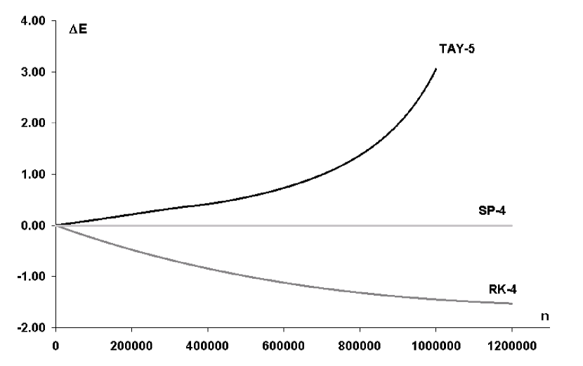
Figure 1: Energy as a function of time ($t=nh$), $h=0.25$, $p_{0}=1.8$, $E_{ex}=0.62$.

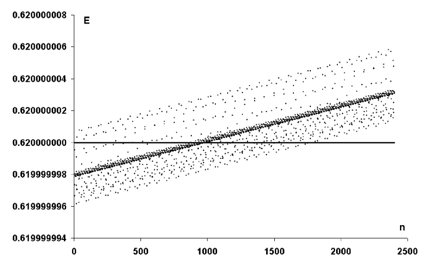
Figure 2: Energy as a function of time ($t=nh$), $h=0.25$, $p_{0}=1.8$, $E_{ex}=0.62$. The line $E=0.62$ corresponds to GR, GR-LEX, GR-3 and GR-7. Other, scattered, points are produced by TAY-10.

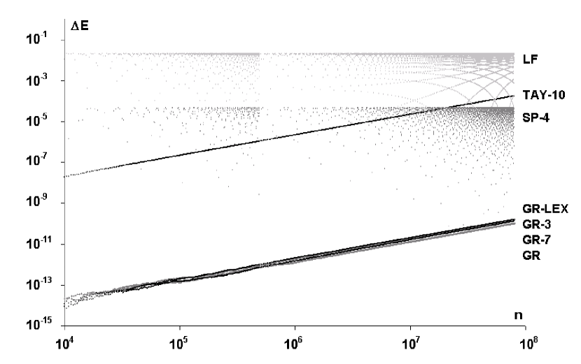
Figure 3: Global error in the energy as a function of time ($t=nh$), $p_{0}=1.8$, $h=0.25$.

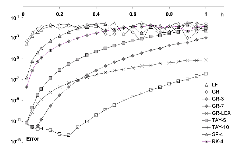
Figure 4: Global error as a function of $h$, evaluated at $t=120T_{th}$ for $p_{0}=0.02$.

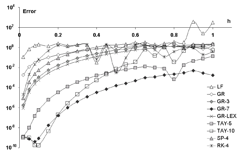
Figure 5: Global error as a function of $h$, evaluated at $t=120T_{th}$ for $p_{0}=1.8$.

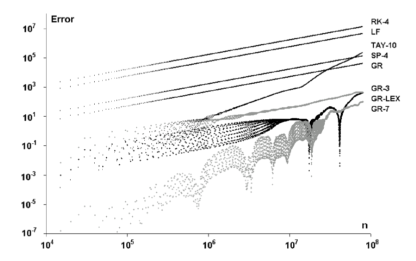
Figure 6: Global error as a function of time ($t=nh$), $p_{0}=2.001$, $h=0.25$.

The accuracy of high-order discrete gradient schemes was tested on the case of the simple pendulum, $H=\frac{1}{2}p^{2}-\cos x$  (for simplicity always assuming $x_{0}=0$). We compared GR-3, GR-7 and GR-LEX with the discrete gradient method (GR), the leap-frog scheme (LF), 4th order explicit Runge-Kutta method (RK-4), high-order Taylor methods (TAY-$N$, see appendix A) and a 4th order symplectic scheme (SP-4, see appendix B). Computing global errors we use the exact solution of the simple pendulum equation, expressed in terms of elliptic integrals.

In previous papers [13, 14, 15] we focused on the stability and accuracy of the period (all motions of the pendulum are periodic). Here, we test the global error, accumulated after $120$ periods (Figures 4 and 5) and the accumulation of error after a very long time (up to $n=10^{8}$ steps), Figure 6. We also check the preservation of the energy integral by different numerical schemes, Figures 1, 2 and 3. Details concerning the solution of implicit equations are the same as in [14], e.g., at every step we iterated until the accuracy $10^{-16}$ was obtained.

Symplectic methods are known to preserve almost exactly the energy integral [19], some positive results in non-symplectic case are also known [16]. Figure 1 shows how accurate is the preservation of the energy by symplectic integrator SP-4 as compared with TAY-5 (permanent, fast growth of the energy) and RK-4 (energy is decreasing approaching the stable equilibrium value). A high order of a given scheme is not sufficient to assure the conservation the energy. From the beginning TAY-10 produces small, but permanent, drift of the energy, while all discrete gradient schemes yield almost exact value of the energy, see Figure 2. According to Theorem 2.1 all gradient schemes preserve the energy integral exactly (up to round-off errors). Only after very long time one can notice that also discrete gradient schemes have a slight drift of the energy. A curious phenomenon can be observed at Figure 3. Gradient schemes and TAY-10 show a linear growth of the energy error (but the energy error of TAY-10 is always greater by 6 orders of magnitude!), while the energy errors of symplectic schemes, LF and SP-4, vary in a large range but do not show any systematic time dependence. However, in the considered time interval, discrete gradient methods preserve the energy more accurately by several orders of magnitude than symplectic integrators like LF or SP-4.

Figures 4, 5  show $h$-dependence of the global error calculated at $t=120T_{ex}$, where $T_{ex}$ is the period of the exact solution (e.g., $T_{ex}=6,283342396$  for  $p_{0}=0.02$ and $T_{ex}=9.12219655$  for  $p_{0}=1.8$). We observe that, usually, higher order integrators are more accurate. An important exception is GR-LEX, of 3rd order, which for $p_{0}=0.02$ and $h>0.3$ is better than GR-7 (the behaviour of GR-SLEX is almost the same as GR-LEX). However, TAY-10 is clearly the best in this case. Only after very long time evolution TAY-10 becomes less accurate than GR and SP-4, although initially it was comparable with gradient schemes of high order, see Figure 6. Several schemes at Figure 6 show linear growth (at least for large $t$). It has been shown, see [7, 19], that symplectic integrators (under some mild conditions) have linear error growth. Results of our experiments suggest that after sufficiently large time some other schemes (e.g., RK-4, GR, GR-3) also accumulate error linearly. Finally, we point out that until $n=10^{7}$ the global error of GR-LEX is smaller than the period (and the error of GR-7 is even smaller, by one order of magintude). The global error of GR is smaller than that of SP-4, not saying about GR-3 or GR-7, see Figure 6.

7 Conclusions

Modifications presented in this paper  essentially improve the discrete gradient method (in the one-dimensional case) keeping all its advantages. Modified gradient schemes GR-LEX, GR-SLEX, GR-$N$ have important advantages:

• conservation of the energy integral (up to round-off errors),

• high stability, exact trajectories in the phase space,

• high accuracy (third, fourth and $N$th order, respectively),

• very good long-time behaviour of numerical solutions.

We point out, however, that numerical schemes (2), like all discrete gradient methods, are neither symplectic nor volume-preserving. Most of them, including GR-LEX and GR-$N$ ($N>2$) are not symmetric (time-reversible). GR and GR-SLEX are symmetric.

In the near future we plan to generalize the approach presented in this paper on some multidimensional cases [11] (the crucial point is that $\delta_{n}$ is a matrix) and to extend the range of its applications on some other numerical integrators (including the implicit midpoint rule and numerical schemes which preserve integrals of motion [25, 29]). One can also use a variable time step, if needed [11].

Appendix A. Explicit Taylor schemes of $N$th order

$N$th Taylor method for the system (1) is defined by

$$x_{n+1}^{[N]}=\sum_{k=0}^{N}\frac{b_{k}h^{k}}{k!}\ ,\qquad p_{n+1}^{[N]}=\sum_{k=0}^{N}\frac{c_{k}h^{k}}{k!}\ ,$$ (31)

where the coefficients $b_{k},c_{k}$ are computed from Taylor’s expansion of the exact solution (see, for instance, [20], p.18). We assume  $x(t)=x_{n}$, $p(t)=p_{n}$, $t=t_{n}$  and expand $x(t+h)$ and $p(t+h)$ in Taylor series:

$$x(t+h)=\sum_{k=0}^{\infty}\frac{b_{k}h^{k}}{k!}\ ,\qquad b_{k}=\left.\frac{d^{k}x(t)}{dt^{k}}\right|_{t=t_{n}}\ ,$$ (32)

$$p(t+h)=\sum_{k=0}^{\infty}\frac{c_{k}h^{k}}{k!}\ ,\qquad c_{k}=\left.\frac{d^{k}p(t)}{dt^{k}}\right|_{t=t_{n}}\ ,$$ (33)

where all derivatives are replaced by functions of $x_{n},p_{n}$  using (1) and its differential consequences, e.g.,

$$\ddot{x}=\frac{d}{dt}\frac{\partial H}{\partial p}=H_{px}{\dot{x}}+H_{pp}{\dot{p}}=H_{px}H_{p}-H_{pp}H_{x}\ ,$$ (34)

where $H_{x},H_{p},H_{xx}$ etc. are evaluated at $x_{n},p_{n}$. Thus we get

$$\begin{array}[]{l}b_{1}=H_{p}\ ,\qquad b_{2}=H_{p}H_{xp}-H_{x}H_{pp}\ ,\\[8.61108pt] b_{3}=H_{x}^{2}H_{3p}+H_{xxp}H_{p}^{2}-2H_{x}H_{p}H_{ppx}+H_{p}H_{xp}^{2}-H_{p}H_{pp}H_{xx}\ ,\\[8.61108pt] c_{1}=-H_{x}\ ,\qquad c_{2}=H_{x}H_{xp}-H_{p}H_{xx}\ ,\\[8.61108pt] c_{3}=-H_{p}^{2}H_{3x}-H_{xpp}H_{x}^{2}+2H_{x}H_{p}H_{xxp}-H_{x}H_{xp}^{2}+H_{x}H_{pp}H_{xx}\ ,\end{array}$$ (35)

and subsequent coefficients can be easily computed using the total derivative:

$$b_{k+1}=\frac{db_{k}}{dt}=H_{p}\frac{\partial b_{k}}{\partial x}-H_{x}\frac{\partial b_{k}}{\partial p}\ ,\qquad c_{k+1}=H_{p}\frac{\partial c_{k}}{\partial x}-H_{x}\frac{\partial c_{k}}{\partial p}\ .$$ (36)

The formulae (35) simplify in the case  $H=T(p)+V(x)$ [15].

Appendix B. Explicit symplectic schemes of $2M$th order

Symplectic explicit integrators of arbitrary even order $N=2M$ can be derived by composition methods, see, e.g., [19]. In this section we present results of the pioneering paper [32], confining ourselves to the case $H=\frac{1}{2}p^{2}+V(x)$.

The numerical scheme SP-2$M$ is defined by the following procedure. Having $x_{n},p_{n}$ we compute the next step, $x_{n+1},p_{n+1}$, as follows. We denote $x_{n}=x^{[0]},p_{n}=p^{[0]}$ and perform $K+1$ iterations (where $K=3^{M-1}$)

$$x^{[i]}=x^{[i-1]}+hc_{M}^{[i]}p^{[i-1]}\ ,\quad p^{[i]}=p^{[i-1]}-hd_{M}^{[i]}V^{\prime}(x^{[i]})\ ,$$ (37)

where $c_{M}^{[i]},d_{M}^{[i]}$ ($i=1,2,\ldots,K+1$) have to be carefully computed (see below) in order to secure the required order. Then we identify $x^{[K+1]}=x_{n+1},p^{[K+1]}=p_{n+1}$.

The coefficients $c_{M}^{[i]},d_{M}^{[i]}$ are computed recursively. First, all coefficients for $M=1$ are given by:

$$c_{1}^{[1]}=\frac{1}{2}\ ,\quad d_{1}^{[1]}=1\ ,\quad c_{1}^{[2]}=\frac{1}{2}\ ,\quad d_{1}^{[2]}=0\ .$$ (38)

Then, we express coefficients $c_{m+1}^{[i]},d_{m+1}^{[i]}$ by coefficients $c_{m}^{[i]},d_{m}^{[i]}$:

$$\begin{array}[]{l}d_{m+1}^{[i]}=d_{m+1}^{[2k+i]}=y_{m}d_{m}^{[i]}\ ,\quad(i=1,\ldots,k)\ ,\\[8.61108pt] d_{m+1}^{[k+i]}=(1-2y_{m})d_{m}^{[i]}\ ,\quad(i=1,\ldots,k)\ ,\\[8.61108pt] d_{m+1}^{[3k+1]}=0\ ,\\[8.61108pt] c_{m+1}^{[i]}=c_{m+1}^{[2k+i+1]}=y_{m}c_{m}^{[i+1]}\ ,\quad(i=1,2,\ldots,k)\ ,\\[8.61108pt] c_{m+1}^{[k+i+1]}=(1-2y_{m})c_{m}^{[i+1]}\ ,\quad(i=1,2,\ldots,k-1)\ ,\\[8.61108pt] c_{m+1}^{[k+1]}=(1-y_{m})\left(c_{m}^{[1]}+c_{m}^{[k+1]}\right)\ ,\\[8.61108pt] c_{m+1}^{[2k+1]}=(1-y_{m})\left(c_{m}^{[1]}+c_{m}^{[k+1]}\right)\ ,\end{array}$$ (39)

where $k=3^{m-1}$ and

$$y_{m}=\frac{1}{2-2^{1/(2m+1)}}\ .$$ (40)

In particular, the symplectic integrator SP-4 has the following coefficients

$$\begin{array}[]{l}\displaystyle c_{2}^{[1]}=c_{2}^{[4]}=\frac{1}{2(2-2^{1/3})}\ ,\quad c_{2}^{[2]}=c_{2}^{[3]}=\frac{1-2^{1/3}}{2(2-2^{1/3})}\ ,\\[12.91663pt] \displaystyle d_{2}^{[1]}=d_{2}^{[3]}=\frac{1}{2-2^{1/3}}\ ,\quad d_{2}^{[2]}=-\frac{2^{1/3}}{2-2^{1/3}}\ ,\quad d_{2}^{[4]}=0\ .\end{array}$$ (41)

The scheme SP-4 was independently presented in [17] and [32].

References

- [1]
- [2]
- [3]
- [4]
- [5] R.P.Agarwal: Difference equations and inequalities (Chapter 3), Marcel Dekker, New York 2000.
- [6] S.Blanes: High order numerical integrators for differential equations using composition and processing of low order methods, Appl. Numer. Math. 37 (2001) 289-306.
- [7] M.P.Calvo, E.Hairer: Accurate long-term integration of dynamical systems, Appl. Numer. Math. 18 (1995) 95-105.
- [8] J.L.Cieśliński: An orbit-preserving discretization of the classical Kepler problem, Phys. Lett. A 370 (2007) 8-12.
- [9] J.L.Cieśliński: On the exact discretization of the classical harmonic oscillator equation, preprint arXiv: 0911.3672v1 [math-ph] (2009); J. Difference Equ. Appl., at press.
- [10] J.L.Cieśliński: Comment on ‘Conservative discretizations of the Kepler motion’, J. Phys. A: Math. Theor. 43 (2010) 228001.
- [11] J.L.Cieśliński: Locally exact modifications of numerical integrators, in preparation.
- [12] J.L.Cieśliński, B.Ratkiewicz: On simulations of the classical harmonic oscillator equation by difference equations, Adv. Difference Eqs. 2006 (2006) 40171.
- [13] J.L.Cieśliński, B.Ratkiewicz: Long-time behaviour of discretizations of the simple pendulum equation, J. Phys. A: Math. Theor. 42 (2009) 105204.
- [14] J.L.Cieśliński, B.Ratkiewicz: Improving the accuracy of the discrete gradient method in the one-dimensional case, Phys. Rev. E 81 (2010) 016704.
- [15] J.L.Cieśliński, B.Ratkiewicz: Discrete gradient algorithms of high order for one-dimensional systems, preprint arXiv: 1008.3895 [physics.comp-ph] (2010);
- [16] E.Faou, E.Hairer, T.L.Pham: Energy conservation with non-symplectic methods: examples and counter-examples, BIT Numer. Math. 44 (2004) 699-709.
- [17] E.Forest, R.D.Ruth: Fourth-order symplectic integration, Physica D 43 (1990) 105-117.
- [18] O.Gonzales: Time integration and discrete Hamiltonian systems, J. Nonl. Sci. 6 (1996) 449-467.
- [19] E.Hairer, C.Lubich, G.Wanner: Geometric numerical integration: structure-preserving algorithms for ordinary differential equations, Second Edition, Springer, Berlin 2006.
- [20] A.Iserles: A first course in the numerical analysis of differential equations, Second Edition, Cambridge Univ. Press 2009.
- [21] T.Itoh, K.Abe: Hamiltonian conserving discrete canonical equations based on variational difference quotients, J. Comput. Phys. 77 (1988) 85-102.
- [22] R.A.LaBudde, D.Greenspan: Discrete mechanics – a general treatment, J. Comput. Phys. 15 (1974) 134-167.
- [23] R.I.McLachlan, G.R.W.Quispel: Splitting methods, Acta Numer. 11 (2002) 341-434.
- [24] R.I.McLachlan, G.R.W.Quispel: Geometric integrators for ODEs, J. Phys. A: Math. Gen. 39 (2006) 5251-5285.
- [25] R.I.McLachlan, G.R.W.Quispel, N.Robidoux: Unified approach to Hamilitonian systems, Poisson systems, gradient systems and systems with Lyapunov functions or first integrals, Phys. Rev. Lett. 81 (1998) 2399-2403.
- [26] R.I.McLachlan, G.R.W.Quispel, N.Robidoux: Geometric integration using discrete gradients, Phil. Trans. R. Soc. London A 357 (1999) 1021-1045.
- [27] R.E.Mickens: Nonstandard finite difference models of differential equations, World Scientific, Singapore 1994.
- [28] R.B.Potts: Differential and difference equations, Am. Math. Monthly 89 (1982) 402-407.
- [29] G.R.W.Quispel, H.W.Capel: Solving ODE’s numerically while preserving a first integral, Phys. Lett. A 218 (1996) 223-228.
- [30] G.R.W.Quispel, G.S.Turner: Discrete gradient methods for solving ODE’s numerically while preserving a first integral, J. Phys. A: Math. Gen. 29 (1996) L341-L349.
- [31] J.C.Simo, N.Tarnow, K.K.Wong: Exact energy-momentum conserving algorithms and symplectic schemes for nonlinear dynamics, Comput. Methods Appl. Mech. Eng. 100 (1992) 63-116.
- [32] H.Yoshida: Construction of higher order symplectic integrators, Phys. Lett. A 150 (1990) 262-268.