Tests of Non-Equivalence among Absolutely Nonsingular Tensors through Geometric Invariants

Sakata, T.1, Maehra, K.2, Sasaki,T.3, Sumi, T. 1, Miyazaki, M.4 and Watanabe Y.5

Department of Design Human Science, Kyushu University1
School of Design, Kyushu University2.
Department of Mathematics, Kobe University3.
Department of Mathematics, Kyoto University of Education4
Research Institute of Information Technology, Kyushu University5

1 Introduction

Tensor data analysis has successfully developed in various application fields, which is useful to seize multi-factor dependence. An nΓ—nΓ—p𝑛𝑛𝑝n\times n\times p tensor is a multi-array datum T=(Ti​j​k),𝑇subscriptπ‘‡π‘–π‘—π‘˜T=(T_{ijk}), where 1≀i,j≀nformulae-sequence1𝑖𝑗𝑛1\leq i,j\leq n and 1≀k≀p.1π‘˜π‘1\leq k\leq p. A type nΓ—nΓ—p𝑛𝑛𝑝n\times n\times p tensor T𝑇T is denoted by T=(A1;A2;β‹―;Ap)𝑇subscript𝐴1subscript𝐴2β‹―subscript𝐴𝑝T=(A_{1};A_{2};\cdots;A_{p}) where Aisubscript𝐴𝑖A_{i} denote nΓ—n𝑛𝑛n\times n matrices. An nΓ—nΓ—p𝑛𝑛𝑝n\times n\times p tensor T𝑇T is said to be of rank 111 if there is a vectors 𝒂=(a1,a2,…,an),𝒂subscriptπ‘Ž1subscriptπ‘Ž2…subscriptπ‘Žπ‘›\bm{a}=(a_{1},a_{2},...,a_{n}), 𝒃=(b1,b2,…,bn)𝒃subscript𝑏1subscript𝑏2…subscript𝑏𝑛\bm{b}=(b_{1},b_{2},...,b_{n}), and 𝒄=(c1,c2,…,cp)𝒄subscript𝑐1subscript𝑐2…subscript𝑐𝑝\bm{c}=(c_{1},c_{2},...,c_{p}) such that Ti​j​k=ai​bj​cksubscriptπ‘‡π‘–π‘—π‘˜subscriptπ‘Žπ‘–subscript𝑏𝑗subscriptπ‘π‘˜T_{ijk}=a_{i}b_{j}c_{k} for all i,j,k,π‘–π‘—π‘˜i,j,k, and the rank of a tensor T𝑇T is defined as the minimum of the integer rπ‘Ÿr such that T𝑇T can be expressed as the sum of rπ‘Ÿr rank-one tensors. The maximal rank of all tensors of type nΓ—nΓ—p𝑛𝑛𝑝n\times n\times p are also defined in obvious fashion and denoted by maxrank​(n,n,p)maxranknnp{\rm maxrank(n,n,p)}.The rank of a tensor describes the complexity of a tensorial datum and the maximal rank describes the model complexity of a class of tensors of a given type, and so they are very important concepts in both applied and theoretical fields. Therefore, the rank and maximal rank determination problems have attracted the interest of many researchers, for example, Kruskal [12], ten-Berge [24], and Common et al, [6], etc. and now have being investigated intensively( for a comprehensive survey, see Kolda et al.[11]). Atkinson et al.([1] and [2] ) claimed that maxrank​(n,n,3)≀2​nβˆ’1maxrank𝑛𝑛32𝑛1{\rm maxrank}(n,n,3)\leq 2n-1. Here we introduce an important class of tensors.

Definition 1.1

A real tensor T=(A1;A2;,…;Ap)T=(A_{1};A_{2};,\dots;A_{p}) is said to be absolutely nonsingular if x1​A1+x2​A2+β‹―+xp​Apsubscriptπ‘₯1subscript𝐴1subscriptπ‘₯2subscript𝐴2β‹―subscriptπ‘₯𝑝subscript𝐴𝑝x_{1}A_{1}+x_{2}A_{2}+\cdots+x_{p}A_{p} is nonsingular for all (x1,x2,…,xp)β‰ (0,0,…,0).subscriptπ‘₯1subscriptπ‘₯2…subscriptπ‘₯𝑝00…0(x_{1},x_{2},...,x_{p})\neq(0,0,...,0).

Remark 1.2

We called absolutely nonsingular tensors as exceptional tensors in Sakata et al. [21],[22].

Sumi et al.[23] proved the claim of Atkinson et al. over the complex number filed β„‚β„‚\mathbb{C} without any assumption and proved it over the real number filed ℝℝ\mathbb{R} except the class of absolutely nonsingular tensors. Thus, for the proof of the claim of Atkinson et al. over the real number filed ℝ,ℝ\mathbb{R}, it is the first thing to determine all absolutely nonsingular tensors. Absolutely nonsingular tensors are characterized by the determinant polynomial defined below. Searching of absolutely nonsingular tensors was pursued in Sakata et al. [21],[22] in this direction. As well as searching absolutely nonsingular tensors, the equivalence among them under the rank-preserving transformation which is defined below is also important. Note that such equivalence relation has also a relation to the SLOCC equivalence of entangled states in the quantum communication (for example, see Chen et al. [5]).
Definition 1.3

For a nΓ—nΓ—p𝑛𝑛𝑝n\times n\times p tensor T=(A1;A2;,…;Ap),T=(A_{1};A_{2};,\dots;A_{p}), the homogeneous polynomial in x1,…,xpsubscriptπ‘₯1…subscriptπ‘₯𝑝x_{1},...,x_{p} of degree n𝑛n

fT​(x1,x2,…,xp)=det(x1​A1+x2​A2+β‹―+xp​Ap)subscript𝑓𝑇subscriptπ‘₯1subscriptπ‘₯2…subscriptπ‘₯𝑝subscriptπ‘₯1subscript𝐴1subscriptπ‘₯2subscript𝐴2β‹―subscriptπ‘₯𝑝subscript𝐴𝑝f_{T}(x_{1},x_{2},...,x_{p})=\det(x_{1}A_{1}+x_{2}A_{2}+\cdots+x_{p}A_{p}) (1.4)

is called the determinant polynomial of a tensor T𝑇T.

Then we have the following important characterization.

Theorem 1.5

If T=(A1;A2;,…;Ap)T=(A_{1};A_{2};,\dots;A_{p}) is absolutely nonsingular, its determinant polynomial fT​(x1,x2,…,xp)subscript𝑓𝑇subscriptπ‘₯1subscriptπ‘₯2…subscriptπ‘₯𝑝f_{T}(x_{1},x_{2},...,x_{p}) is a positive definite homogeneous polynomial or negative definite homogeneous polynomial.

Proof  Let T=(A1;A2;,…;Ap)T=(A_{1};A_{2};,\dots;A_{p}) be absolutely nonsingular, and assume that there are two points 𝒙0subscript𝒙0\bm{x}_{0} and 𝒙1subscript𝒙1\bm{x}_{1} such that fT​(𝒙0)>0subscript𝑓𝑇subscript𝒙00f_{T}(\bm{x}_{0})>0 and fT​(𝒙1)<0.subscript𝑓𝑇subscript𝒙10f_{T}(\bm{x}_{1})<0. The line β„“β„“\ell combining the two points 𝒙0subscript𝒙0\bm{x}_{0} and 𝒙1subscript𝒙1\bm{x}_{1} must pass through the origin 𝟎0\bm{0}, since in the segment [x0,x1]subscriptπ‘₯0subscriptπ‘₯1[x_{0},x_{1}] there must be 𝒙′superscript𝒙′\bm{x}^{\prime} such that fT​(𝒙′)=0subscript𝑓𝑇superscript𝒙′0f_{T}(\bm{x}^{\prime})=0 and it must be 𝟎0\bm{0} because T𝑇T is absolutely nonsingular. Let take another point 𝒙2subscript𝒙2\bm{x}_{2} which is not on the line β„“β„“\ell. Then, the line passing 𝒙0subscript𝒙0\bm{x}_{0} and 𝒙2subscript𝒙2\bm{x}_{2} does not pass the origin and so f​(𝒙0)​f​(𝒙2)<0𝑓subscript𝒙0𝑓subscript𝒙20f(\bm{x}_{0})f(\bm{x}_{2})<0 is impossible just by the same reason given in the previous sentence. So, f​(𝒙0)​f​(𝒙2)>0.𝑓subscript𝒙0𝑓subscript𝒙20f(\bm{x}_{0})f(\bm{x}_{2})>0. Next, consider the line passing 𝒙1subscript𝒙1\bm{x}_{1} and 𝒙2subscript𝒙2\bm{x}_{2}, which also does not pass the origin and f​(𝒙1)​f​(𝒙2)<0𝑓subscript𝒙1𝑓subscript𝒙20f(\bm{x}_{1})f(\bm{x}_{2})<0. This is also a contradiction. After all, there don’t exist points 𝒙0subscript𝒙0\bm{x}_{0} and 𝒙1subscript𝒙1\bm{x}_{1} such that f​(𝒙0)>0𝑓subscript𝒙00f(\bm{x}_{0})>0 and f​(𝒙1)<0.𝑓subscript𝒙10f(\bm{x}_{1})<0. This proves Theorem 1.5. Β 

It is well known that tensor rank is invariant by typical matrix transformations, say, pβˆ’limit-from𝑝p-, qβˆ’limit-fromπ‘žq-, and rβˆ’limit-fromπ‘Ÿr-transformations defined below. So, equivalence relation of two tensors means that they have a same rank. Thus, to study equivalence among tensors is of some importance for rank determination.

Definition 1.6

For a nΓ—nΓ—p𝑛𝑛𝑝n\times n\times p tensor T=(A1;A2;β‹―;Ap),𝑇subscript𝐴1subscript𝐴2β‹―subscript𝐴𝑝T=(A_{1};A_{2};\cdots;A_{p}), the following transformations

  • (1)

    T=(A1;A2;β‹―;Ap)β†’Tβ€²=(P​A1;P​A2;β‹―;P​Ap)𝑇subscript𝐴1subscript𝐴2β‹―subscript𝐴𝑝→superscript𝑇′𝑃subscript𝐴1𝑃subscript𝐴2⋯𝑃subscript𝐴𝑝T=(A_{1};A_{2};\cdots;A_{p})\rightarrow T^{\prime}=(PA_{1};PA_{2};\cdots;PA_{p}) by an nΓ—n𝑛𝑛n\times n matrix P∈G​L​(n),𝑃𝐺𝐿𝑛P\in GL(n),

  • (2)

    T=(A1;A2;β‹―;Ap)β†’Tβ€²=(A1​Q;P​A2​Q;β‹―;Ap​Q)𝑇subscript𝐴1subscript𝐴2β‹―subscript𝐴𝑝→superscript𝑇′subscript𝐴1𝑄𝑃subscript𝐴2𝑄⋯subscript𝐴𝑝𝑄T=(A_{1};A_{2};\cdots;A_{p})\rightarrow T^{\prime}=(A_{1}Q;PA_{2}Q;\cdots;A_{p}Q) by an nΓ—n𝑛𝑛n\times n matrix P∈G​L​(n),𝑃𝐺𝐿𝑛P\in GL(n),

  • (3)

    T=(A1;A2;β‹―;Ap)β†’Tβ€²=(R11​A1+R12​A2+R13​A3;R21​A1+R22​A2+R23​A3;R31​A1+R32​A2+R33​A3)𝑇subscript𝐴1subscript𝐴2β‹―subscript𝐴𝑝→superscript𝑇′subscript𝑅11subscript𝐴1subscript𝑅12subscript𝐴2subscript𝑅13subscript𝐴3subscript𝑅21subscript𝐴1subscript𝑅22subscript𝐴2subscript𝑅23subscript𝐴3subscript𝑅31subscript𝐴1subscript𝑅32subscript𝐴2subscript𝑅33subscript𝐴3T=(A_{1};A_{2};\cdots;A_{p})\rightarrow T^{\prime}=(R_{11}A_{1}+R_{12}A_{2}+R_{13}A_{3};R_{21}A_{1}+R_{22}A_{2}+R_{23}A_{3};R_{31}A_{1}+R_{32}A_{2}+R_{33}A_{3}) by a pΓ—p𝑝𝑝p\times p matrix P∈G​L​(n)𝑃𝐺𝐿𝑛P\in GL(n)

are called as pβˆ’limit-from𝑝p-, qβˆ’limit-fromπ‘žq-, and rβˆ’limit-fromπ‘Ÿr-transformations and denoted by Tβ†’pTβ€²,Tβ†’qT′​a​n​d​Tβ†’rTβ€²formulae-sequencesubscript→𝑝𝑇superscript𝑇′subscriptβ†’π‘žπ‘‡superscriptπ‘‡β€²π‘Žπ‘›π‘‘π‘‡subscriptβ†’π‘Ÿsuperscript𝑇′T\rightarrow_{p}T^{\prime},T\rightarrow_{q}T^{\prime}andT\rightarrow_{r}T^{\prime} respectively. Further, if T1β†’pT2subscript→𝑝subscript𝑇1subscript𝑇2T_{1}\rightarrow_{p}T_{2}, the T1subscript𝑇1T_{1} and T2subscript𝑇2T_{2} are said to be in the pβˆ’limit-from𝑝p-equivalence. qβˆ’limit-fromπ‘žq- and rβˆ’limit-fromπ‘Ÿr-equivalence are defined analogously.

Definition 1.7

Let T1=(A1;A2;β‹―;Ap)subscript𝑇1subscript𝐴1subscript𝐴2β‹―subscript𝐴𝑝T_{1}=(A_{1};A_{2};\cdots;A_{p}) and T2=(B1;B2;β‹―;Bp)subscript𝑇2subscript𝐡1subscript𝐡2β‹―subscript𝐡𝑝T_{2}=(B_{1};B_{2};\cdots;B_{p}) be two nΓ—nΓ—p𝑛𝑛𝑝n\times n\times p tensors. If there is a sequence of {Ti}subscript𝑇𝑖\{T_{i}\} starting from T1subscript𝑇1T_{1} and ending at T2,subscript𝑇2T_{2}, in which Tisubscript𝑇𝑖T_{i} and Ti+1subscript𝑇𝑖1T_{i+1} are in the relation of pβˆ’limit-from𝑝p-, or qβˆ’limit-fromπ‘žq-, or rβˆ’limit-fromπ‘Ÿr-equivalence, then T0subscript𝑇0T_{0} and T1subscript𝑇1T_{1} are said to be equivalent.

Now we can reduce the equivalence relation into a more simple one by the following lemma.

Lemma 1.8

pβˆ’limit-from𝑝p-, qβˆ’limit-fromπ‘žq- and rβˆ’limit-fromπ‘Ÿr-transformations are mutually commutative.

Proof  For simplicity, we prove for p=3𝑝3p=3, however, the proof is similar for a general p𝑝p. First we prove the commutativity of pβˆ’limit-from𝑝p-transformation and rβˆ’limit-fromπ‘Ÿr-transformation. Let

T1β†’pT2β†’rT3a​n​dT1β†’rT2β€²β†’pT3β€²formulae-sequencesubscript→𝑝subscript𝑇1subscript𝑇2subscriptβ†’π‘Ÿsubscript𝑇3subscriptβ†’π‘Ÿπ‘Žπ‘›π‘‘subscript𝑇1subscriptsuperscript𝑇′2subscript→𝑝subscriptsuperscript𝑇′3T_{1}\rightarrow_{p}T_{2}\rightarrow_{r}T_{3}\ \ and\ \ T_{1}\rightarrow_{r}T^{{}^{\prime}}_{2}\rightarrow_{p}T^{{}^{\prime}}_{3}

We will show that T3=T3β€².subscript𝑇3subscriptsuperscript𝑇′3T_{3}=T^{{}^{\prime}}_{3}. Let T1=(A1;A2;A3)subscript𝑇1subscript𝐴1subscript𝐴2subscript𝐴3T_{1}=(A_{1};A_{2};A_{3}) and P=(pi​j)𝑃subscript𝑝𝑖𝑗P=(p_{ij}) and R=(ri​j).𝑅subscriptπ‘Ÿπ‘–π‘—R=(r_{ij}). Then,

T2=(P​A1;P​A2;P​A3)subscript𝑇2𝑃subscript𝐴1𝑃subscript𝐴2𝑃subscript𝐴3T_{2}=(PA_{1};PA_{2};PA_{3})

and

T3=(r11​P​A1+r12​P​A2+r13​P​A3;r21​P​A1+r22​P​A2+r23​P​A3;r31​P​A1+r32​P​A2+r33​P​A3)subscript𝑇3subscriptπ‘Ÿ11𝑃subscript𝐴1subscriptπ‘Ÿ12𝑃subscript𝐴2subscriptπ‘Ÿ13𝑃subscript𝐴3subscriptπ‘Ÿ21𝑃subscript𝐴1subscriptπ‘Ÿ22𝑃subscript𝐴2subscriptπ‘Ÿ23𝑃subscript𝐴3subscriptπ‘Ÿ31𝑃subscript𝐴1subscriptπ‘Ÿ32𝑃subscript𝐴2subscriptπ‘Ÿ33𝑃subscript𝐴3T_{3}=(r_{11}PA_{1}+r_{12}PA_{2}+r_{13}PA_{3};r_{21}PA_{1}+r_{22}PA_{2}+r_{23}PA_{3};r_{31}PA_{1}+r_{32}PA_{2}+r_{33}PA_{3})

On the other hand

T2β€²=(r11​A1+r12​A2+r13​A3;r21​A1+r22​A2+r23​A3;r31​A1+r32​A2+r33​A3)subscriptsuperscript𝑇′2subscriptπ‘Ÿ11subscript𝐴1subscriptπ‘Ÿ12subscript𝐴2subscriptπ‘Ÿ13subscript𝐴3subscriptπ‘Ÿ21subscript𝐴1subscriptπ‘Ÿ22subscript𝐴2subscriptπ‘Ÿ23subscript𝐴3subscriptπ‘Ÿ31subscript𝐴1subscriptπ‘Ÿ32subscript𝐴2subscriptπ‘Ÿ33subscript𝐴3T^{{}^{\prime}}_{2}=(r_{11}A_{1}+r_{12}A_{2}+r_{13}A_{3};r_{21}A_{1}+r_{22}A_{2}+r_{23}A_{3};r_{31}A_{1}+r_{32}A_{2}+r_{33}A_{3})

and

T3β€²=(r11​P​A1+r12​P​A2+r13​P​A3;r21​P​A1+r22​P​A2+r23​P​A3;r31​P​A1+r32​P​A2+r33​P​A3)subscriptsuperscript𝑇′3subscriptπ‘Ÿ11𝑃subscript𝐴1subscriptπ‘Ÿ12𝑃subscript𝐴2subscriptπ‘Ÿ13𝑃subscript𝐴3subscriptπ‘Ÿ21𝑃subscript𝐴1subscriptπ‘Ÿ22𝑃subscript𝐴2subscriptπ‘Ÿ23𝑃subscript𝐴3subscriptπ‘Ÿ31𝑃subscript𝐴1subscriptπ‘Ÿ32𝑃subscript𝐴2subscriptπ‘Ÿ33𝑃subscript𝐴3T^{{}^{\prime}}_{3}=(r_{11}PA_{1}+r_{12}PA_{2}+r_{13}PA_{3};r_{21}PA_{1}+r_{22}PA_{2}+r_{23}PA_{3};r_{31}PA_{1}+r_{32}PA_{2}+r_{33}PA_{3})

Thus, T3=T3β€²,subscript𝑇3subscriptsuperscript𝑇′3T_{3}=T^{{}^{\prime}}_{3}, and this means the commutativity of p𝑝p- and rπ‘Ÿr-transformations. The commutativity of qπ‘žq- and rπ‘Ÿr-transformations are proved similarly. p𝑝p- and qπ‘žq-transformations are obviously commutative. This proves Lemma 1.8. Β 

Note that in this paper we consider three cases of (1) P,Q∈G​L​(n)𝑃𝑄𝐺𝐿𝑛P,Q\in GL(n) and R∈G​L​(p)𝑅𝐺𝐿𝑝R\in GL(p) and (2) P,Q∈G​L​(n)𝑃𝑄𝐺𝐿𝑛P,Q\in GL(n) and R∈S​L​(p).𝑅𝑆𝐿𝑝R\in SL(p). and (3) P,Q∈S​L​(n)𝑃𝑄𝑆𝐿𝑛P,Q\in SL(n) and R∈S​L​(p).𝑅𝑆𝐿𝑝R\in SL(p). The first is called G​L​(p)𝐺𝐿𝑝GL(p)-equivalence or simply equivalence, and the second is called S​L​(p)𝑆𝐿𝑝SL(p)-equivalence in short. The third case is called, in a full term, S​L​(n)Γ—S​L​(n)Γ—S​L​(p)𝑆𝐿𝑛𝑆𝐿𝑛𝑆𝐿𝑝SL(n)\times SL(n)\times SL(p)-equivalence. Lemma 1.8 implies the following theorem.

Theorem 1.9

T1subscript𝑇1T_{1} and T2subscript𝑇2T_{2} are G​L​(p)𝐺𝐿𝑝GL(p)-equivalent if and only if there is a set of p𝑝p-transformation, qπ‘žq-transformation and rπ‘Ÿr-transformation such that

T1β†’pTβ€²β†’qT"β†’rT2subscript→𝑝subscript𝑇1superscript𝑇′subscriptβ†’π‘žsuperscript𝑇"subscriptβ†’π‘Ÿsubscript𝑇2T_{1}\rightarrow_{p}T^{{}^{\prime}}\rightarrow_{q}T^{"}\rightarrow_{r}T_{2}

Thus, the equivalence problem of tensors T1=(A1(1):,,,:Ap(1))T_{1}=(A^{(1)}_{1}:,,,:A^{(1)}_{p}) and T2=(A1(2):,,,:Ap(2))T_{2}=(A^{(2)}_{1}:,,,:A^{(2)}_{p}) is reduced to the problem whether the following system of algebraic equations for P𝑃P, Q𝑄Q and R𝑅R can have a solution or not.

Ai(2)=P({βˆ‘j=1pri​jAj(1)}Q,i=1,2,…,pA^{(2)}_{i}=P(\{\sum_{j=1}^{p}r_{ij}A^{(1)}_{j}\}Q,i=1,2,...,p (1.10)

These algebraic equations have too many variables to solve even when the size of matrices Aisubscript𝐴𝑖A_{i} is moderate. So, in this paper, we propose to see the problem through the determinant polynomial. Then, though we necessarily have to discard the sufficiency part of the problem, however, the problem becomes concise and tractable one by the following proposition.

Proposition 1.11

If T1subscript𝑇1T_{1} and T2subscript𝑇2T_{2} are G​L​(p)𝐺𝐿𝑝GL(p)-equivalent, it holds that there is a constant cβˆˆβ„π‘β„c\in\mathbb{R} and a pΓ—p𝑝𝑝p\times p nonsingular matrix R∈G​L​(p)𝑅𝐺𝐿𝑝R\in GL(p) such that

fT2​(𝒙)=c​fT1​(𝒙​R)subscript𝑓subscript𝑇2𝒙𝑐subscript𝑓subscript𝑇1𝒙𝑅f_{T_{2}}(\bm{x})=cf_{T_{1}}(\bm{x}R) (1.12)

So, we can say that

Proposition 1.13

For two tensors, if the equation (1.12) does not hold for any constant cβˆˆβ„π‘β„c\in\mathbb{R} and any matrix R∈G​L​(p)𝑅𝐺𝐿𝑝R\in GL(p), they are not G​L​(p)𝐺𝐿𝑝GL(p)-equivalent.

Though the reduced equation (1.12) happens to be solved algebraically in some cases. However, it is still hard to solve, in general, a system of algebraic equation with too many variables. In fact, we need to decide whether a system of (n+1)​(n+2)2𝑛1𝑛22\frac{(n+1)(n+2)}{2} homogeneous equations with (p2+1)superscript𝑝21(p^{2}+1) variables of degree n𝑛n have a solution or not. So, in this paper, we avoid to solve the problem algebraically and propose to attack the problem from a geometric view point, that is, we propose to test non equivalence by checking whether the two surfaces of the determinant polynomials of T1subscript𝑇1T_{1} and T2subscript𝑇2T_{2} have a same geometric invariants, or not. Here, multi-linear algebra and differential geometry intersect through the widow of determinant polynomials.
The first aim of this paper is to show theoretically that differential geometric invariants are useful as testers of non-equivalence among absolutely nonsingular tensors. The second aim is to show that we can calculate the values of the invariants with enough accuracy. Third, we compare the values of invariants calculated by the lattice method and by the t-design method. And it is shown that the lattice point method gives more stable values than the t-design method. As S​L​(p)𝑆𝐿𝑝SL(p)-invariant, we consider first the volume enclosed by the constant surface and then we consider the affine surface area, and thirdly we consider the Lpsuperscript𝐿𝑝L^{p} affine surface area of convex body. Affine surface area was studied by Blaschke [4] and extended to Lpsubscript𝐿𝑝L_{p} affine surface area by Lutwak [20], (also see Leichtwess [13]). As for a valuation theory of Lpsubscript𝐿𝑝L_{p} affine surface area, see the recent papers by Ludwig [15] and Ludwig and Reitzer [17]. Finally, as a general reference of affine differential geometry, see K. Nomizu and T. Sasaki [19].
This paper is organized as follows. In Section 2, we show how to parametrize the constant surface of a determinant polynomial and in Section 3, we review briefly some definitions from differential geometry. In Section 4, we argue rough S​L​(p)𝑆𝐿𝑝SL(p)-invariants. In Section 5, we deal with S​L​(p)𝑆𝐿𝑝SL(p)-invariant. In the first subsection, we introduce the valuation theory for the set of convex bodies and in the second subsection, we argue a volume of the region enclosed by a constant surface as an S​L​(p)𝑆𝐿𝑝SL(p)-invariant. In the third subsection, we argue the affine surface as a S​L​(p)𝑆𝐿𝑝SL(p)-invariant. In Section 6, we consider the generalized affine surface, that is, Lpsubscript𝐿𝑝L_{p} affine surface area, especially centro-affine surface as a G​L​(p)𝐺𝐿𝑝GL(p)-invariant. In Section 7, we review the theory of spherical t-design briefly and give a theorem important for approximate calculation of our proposed invariants. In Section 8, we give numerical values of the invariants calculated by the lattice method and t-design method. It is shown numerically that the proposed invariants is usefull to discriminate non equivalence. In Section 9, the conclusion is given. Finally note that in the following we consider mainly the case of n=4𝑛4n=4 and p=3,𝑝3p=3, though some statements are given for general n𝑛n and p.𝑝p. One reason is that absolutely nonsingular tensors are not so easy to obtain for general cases and the second reason is because it is easy to see that our method is also available for general cases. The study of much higher values of n𝑛n and p𝑝p will be given in the future work.

2 Parametrization of constant surface

The determinant polynomial of a 4Γ—4Γ—34434\times 4\times 3 tensor T=(A1;A2;A3)𝑇subscript𝐴1subscript𝐴2subscript𝐴3T=(A_{1};A_{2};A_{3}), ifT​(x,y,z)=d​e​t​(x​A1+y​A2+z​A3),subscript𝑓𝑇π‘₯𝑦𝑧𝑑𝑒𝑑π‘₯subscript𝐴1𝑦subscript𝐴2𝑧subscript𝐴3f_{T}(x,y,z)=det(xA_{1}+yA_{2}+zA_{3}), is a homogeneous polynomial of three variables with degree 4. We are concerned with the integral invariants of the constant surface βˆ‚Ξ©T={(x,y,z)|fT​(x,y,z)=1}subscriptΩ𝑇conditional-setπ‘₯𝑦𝑧subscript𝑓𝑇π‘₯𝑦𝑧1\partial\Omega_{T}=\{(x,y,z)|f_{T}(x,y,z)=1\} for the special linear group S​L​(3)𝑆𝐿3SL(3) and the general linear group G​L​(3)𝐺𝐿3GL(3). To get such invariants, we need to parametrize this surface by the usual spherical coordinate,

xπ‘₯\displaystyle x =\displaystyle= r​sin⁑s​cos⁑t=r​Φx​(s,t)π‘Ÿπ‘ π‘‘π‘ŸsubscriptΞ¦π‘₯𝑠𝑑\displaystyle r\sin s\cos t=r\Phi_{x}(s,t) (2.1)
y𝑦\displaystyle y =\displaystyle= r​sin⁑s​sin⁑t=r​Φy​(s,t)π‘Ÿπ‘ π‘‘π‘ŸsubscriptΦ𝑦𝑠𝑑\displaystyle r\sin s\sin t=r\Phi_{y}(s,t) (2.2)
z𝑧\displaystyle z =\displaystyle= r​cos⁑s=r​Φz​(s,t),π‘Ÿπ‘ π‘ŸsubscriptΦ𝑧𝑠𝑑\displaystyle r\cos s=r\Phi_{z}(s,t), (2.3)

where 0<s<Ο€,0<t<2​π.formulae-sequence0π‘ πœ‹0𝑑2πœ‹0<s<\pi,0<t<2\pi. Let 𝒙𝒙\bm{x} denote the point (x,y,z)π‘₯𝑦𝑧(x,y,z) on the surface. Putting these into the equation fT​(x,y,z)=1,subscript𝑓𝑇π‘₯𝑦𝑧1f_{T}(x,y,z)=1, we have

r4=1p​(s,t),superscriptπ‘Ÿ41𝑝𝑠𝑑r^{4}=\frac{1}{p(s,t)}, (2.4)

where

p​(s,t)=fT​(Ξ¦x​(s,t),Ξ¦y​(s,t),Ξ¦z​(s,t)).𝑝𝑠𝑑subscript𝑓𝑇subscriptΞ¦π‘₯𝑠𝑑subscriptΦ𝑦𝑠𝑑subscriptΦ𝑧𝑠𝑑p(s,t)=f_{T}(\Phi_{x}(s,t),\Phi_{y}(s,t),\Phi_{z}(s,t)). (2.5)

And so,

𝒙=1p​(s,t)1/4​(Ξ¦x​(s,t),Ξ¦y​(s,t),Ξ¦z​(s,t)).𝒙1𝑝superscript𝑠𝑑14subscriptΞ¦π‘₯𝑠𝑑subscriptΦ𝑦𝑠𝑑subscriptΦ𝑧𝑠𝑑\bm{x}=\frac{1}{p(s,t)^{1/4}}\left(\Phi_{x}(s,t),\Phi_{y}(s,t),\Phi_{z}(s,t)\right). (2.6)

This equation (2.6) gives a parametric representation of the constant surface βˆ‚Ξ©TsubscriptΩ𝑇\partial\Omega_{T}. Then, the following is a starting point of this research of the constant surface.

Theorem 2.7

The constant surface of the determinant polynomial of an absolutely nonsingular tensor is a compact set in ℝ3superscriptℝ3\mathbb{R}^{3} without self-intersection.

Proof  Without loss of generality, we assume that fT​(𝒙)subscript𝑓𝑇𝒙f_{T}(\bm{x}) is positive definite. If π’™βˆˆβˆ‚Ξ©T𝒙subscriptΩ𝑇\bm{x}\in\partial\Omega_{T}, for any 0<r<10π‘Ÿ10<r<1 and r>1,π‘Ÿ1r>1, rβ€‹π’™π‘Ÿπ’™r\bm{x} is not in βˆ‚Ξ©T.subscriptΩ𝑇\partial\Omega_{T}. That is, the constant surface is of a star-shaped. This proves that the surface has not any self intersection. Since p​(s,t)𝑝𝑠𝑑p(s,t) is continuous on the unit sphere it takes a positive minimum and a positive maximum. So, 𝒙𝒙\bm{x} in the equation 2.6 is bounded, which implies the compactness of the constant surface. This completes the proof of Theorem 2.7. Β 

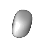
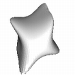
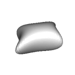
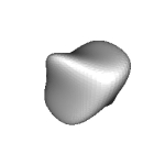
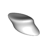
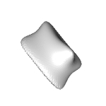
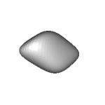
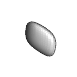
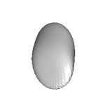
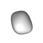
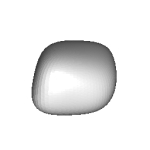
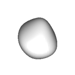
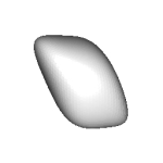
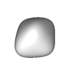
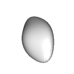
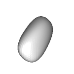
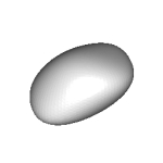
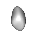
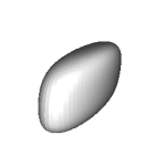
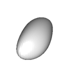
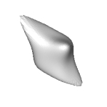
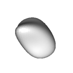
The following 8 figures are examples of the constant surfaces of 4Γ—4Γ—34434\times 4\times 3 absolutely nonsingular tensors.

Refer to caption
Refer to caption
Refer to caption
Refer to caption
Refer to caption
Refer to caption
Refer to caption
Refer to caption
Figure 1: Constant surfaces of the determinant polynomials of tensors FN​o​1,3,10,20,99,119,207,237.π‘π‘œ13102099119207237No1,3,10,20,99,119,207,237.

Note that the numbering of tensors is based on the list of nonsingular tensors with elements consisting only of βˆ’1,0,1101-1,0,1 found by us. Each figure corresponds to the following tensor and its determinant function respectively.

T1=(1000010000100001):(βˆ’10111βˆ’11βˆ’1βˆ’1βˆ’1βˆ’1βˆ’10110):(01βˆ’110βˆ’1110βˆ’10βˆ’1βˆ’1βˆ’111),:subscript𝑇110000100001000011011111111110110:0111011101011111T_{1}=\left(\begin{array}[]{cccc}1&0&0&0\\ 0&1&0&0\\ 0&0&1&0\\ 0&0&0&1\\ \end{array}\right):\left(\begin{array}[]{cccc}-1&0&1&1\\ 1&-1&1&-1\\ -1&-1&-1&-1\\ 0&1&1&0\\ \end{array}\right):\left(\begin{array}[]{cccc}0&1&-1&1\\ 0&-1&1&1\\ 0&-1&0&-1\\ -1&-1&1&1\\ \end{array}\right),
fT1​(x,y,z)subscript𝑓subscript𝑇1π‘₯𝑦𝑧\displaystyle f_{T_{1}}(x,y,z) =\displaystyle= x4+6y4+2z4+βˆ’3x3yβˆ’8xy3βˆ’3xz3+5z3y+\displaystyle x^{4}+6y^{4}+2z^{4}+-3x^{3}y-8xy^{3}-3xz^{3}+5z^{3}y+
7​x2​y2+3​x2​z2+8​z2​y2βˆ’2​x​y2​zβˆ’8​x​y​z2.7superscriptπ‘₯2superscript𝑦23superscriptπ‘₯2superscript𝑧28superscript𝑧2superscript𝑦22π‘₯superscript𝑦2𝑧8π‘₯𝑦superscript𝑧2\displaystyle 7x^{2}y^{2}+3x^{2}z^{2}+8z^{2}y^{2}-2xy^{2}z-8xyz^{2}.
T3=(1000010000100001):(01000βˆ’10110βˆ’0βˆ’11βˆ’11):(1111βˆ’100βˆ’10βˆ’100βˆ’11βˆ’11),:subscript𝑇31000010000100001010001011001111:1111100101001111T_{3}=\left(\begin{array}[]{cccc}1&0&0&0\\ 0&1&0&0\\ 0&0&1&0\\ 0&0&0&1\\ \end{array}\right):\left(\begin{array}[]{cccc}0&1&0&0\\ 0&-1&0&1\\ 1&0&-&0\\ -1&1&-1&1\\ \end{array}\right):\left(\begin{array}[]{cccc}1&1&1&1\\ -1&0&0&-1\\ 0&-1&0&0\\ -1&1&-1&1\\ \end{array}\right),
fT3​(x,y,z)subscript𝑓subscript𝑇3π‘₯𝑦𝑧\displaystyle f_{T_{3}}(x,y,z) =\displaystyle= x4+3​y4+6​z4βˆ’3​x3​z+2​x​y3+4​y3​zsuperscriptπ‘₯43superscript𝑦46superscript𝑧43superscriptπ‘₯3𝑧2π‘₯superscript𝑦34superscript𝑦3𝑧\displaystyle x^{4}+3y^{4}+6z^{4}-3x^{3}z+2xy^{3}+4y^{3}z
βˆ’7​x​z3βˆ’6​z3​y+x2​y2+5​x2​z2βˆ’5​z2​y2+4​x​y2​zβˆ’x2​y​z+2​x​y​z2.7π‘₯superscript𝑧36superscript𝑧3𝑦superscriptπ‘₯2superscript𝑦25superscriptπ‘₯2superscript𝑧25superscript𝑧2superscript𝑦24π‘₯superscript𝑦2𝑧superscriptπ‘₯2𝑦𝑧2π‘₯𝑦superscript𝑧2\displaystyle-7xz^{3}-6z^{3}y+x^{2}y^{2}+5x^{2}z^{2}-5z^{2}y^{2}+4xy^{2}z-x^{2}yz+2xyz^{2}.
T10=(1000010000100001):(01000βˆ’101101000βˆ’1βˆ’1):(1111βˆ’100βˆ’10βˆ’100βˆ’11βˆ’11),:subscript𝑇1010000100001000010100010110100011:1111100101001111T_{10}=\left(\begin{array}[]{cccc}1&0&0&0\\ 0&1&0&0\\ 0&0&1&0\\ 0&0&0&1\\ \end{array}\right):\left(\begin{array}[]{cccc}0&1&0&0\\ 0&-1&0&1\\ 1&0&1&0\\ 0&0&-1&-1\\ \end{array}\right):\left(\begin{array}[]{cccc}1&1&1&1\\ -1&0&0&-1\\ 0&-1&0&0\\ -1&1&-1&1\\ \end{array}\right),
fT10​(x,y,z)=x4+y4+2​z4βˆ’x3​y+2​x3​z+x​y3+2​x​z3subscript𝑓subscript𝑇10π‘₯𝑦𝑧superscriptπ‘₯4superscript𝑦42superscript𝑧4superscriptπ‘₯3𝑦2superscriptπ‘₯3𝑧π‘₯superscript𝑦32π‘₯superscript𝑧3\displaystyle f_{T_{10}}(x,y,z)=x^{4}+y^{4}+2z^{4}-x^{3}y+2x^{3}z+xy^{3}+2xz^{3}
βˆ’z3​yβˆ’x2​y2+4​x2​z2βˆ’2​x​y2​zβˆ’2​x2​y​zβˆ’x​y​z2.superscript𝑧3𝑦superscriptπ‘₯2superscript𝑦24superscriptπ‘₯2superscript𝑧22π‘₯superscript𝑦2𝑧2superscriptπ‘₯2𝑦𝑧π‘₯𝑦superscript𝑧2\displaystyle-z^{3}y-x^{2}y^{2}+4x^{2}z^{2}-2xy^{2}z-2x^{2}yz-xyz^{2}.
T20=(1000010000100001):(βˆ’101βˆ’100011βˆ’1001000):(1011111βˆ’100011βˆ’1βˆ’1βˆ’1),:subscript𝑇2010000100001000011011000111001000:1011111100011111T_{20}=\left(\begin{array}[]{cccc}1&0&0&0\\ 0&1&0&0\\ 0&0&1&0\\ 0&0&0&1\\ \end{array}\right):\left(\begin{array}[]{cccc}-1&0&1&-1\\ 0&0&0&1\\ 1&-1&0&0\\ 1&0&0&0\\ \end{array}\right):\left(\begin{array}[]{cccc}1&0&1&1\\ 1&1&1&-1\\ 0&0&0&1\\ 1&-1&-1&-1\\ \end{array}\right),
fT20​(x,y,z)=x4+y4+2​z4βˆ’x3​y+x3​z+y3​zβˆ’x​z3+2​z3​y+subscript𝑓subscript𝑇20π‘₯𝑦𝑧superscriptπ‘₯4superscript𝑦42superscript𝑧4superscriptπ‘₯3𝑦superscriptπ‘₯3𝑧superscript𝑦3𝑧π‘₯superscript𝑧3limit-from2superscript𝑧3𝑦\displaystyle f_{T_{20}}(x,y,z)=x^{4}+y^{4}+2z^{4}-x^{3}y+x^{3}z+y^{3}z-xz^{3}+2z^{3}y+
βˆ’x2​z2+6​z2​y2+x​y2​z+x2​y​z+2​x​y​z2.superscriptπ‘₯2superscript𝑧26superscript𝑧2superscript𝑦2π‘₯superscript𝑦2𝑧superscriptπ‘₯2𝑦𝑧2π‘₯𝑦superscript𝑧2\displaystyle-x^{2}z^{2}+6z^{2}y^{2}+xy^{2}z+x^{2}yz+2xyz^{2}.
T99=(1000010000100001):(0βˆ’1βˆ’1βˆ’1111βˆ’11βˆ’110βˆ’11βˆ’11):(01000βˆ’111101βˆ’11011),:subscript𝑇9910000100001000010111111111101111:0100011110111011T_{99}=\left(\begin{array}[]{cccc}1&0&0&0\\ 0&1&0&0\\ 0&0&1&0\\ 0&0&0&1\\ \end{array}\right):\left(\begin{array}[]{cccc}0&-1&-1&-1\\ 1&1&1&-1\\ 1&-1&1&0\\ -1&1&-1&1\\ \end{array}\right):\left(\begin{array}[]{cccc}0&1&0&0\\ 0&-1&1&1\\ 1&0&1&-1\\ 1&0&1&1\\ \end{array}\right),
fT99​(x,y,z)=x4+2​y4+2​z4+3​x3​y+x3​z+3​x​y3+subscript𝑓subscript𝑇99π‘₯𝑦𝑧superscriptπ‘₯42superscript𝑦42superscript𝑧43superscriptπ‘₯3𝑦superscriptπ‘₯3𝑧limit-from3π‘₯superscript𝑦3\displaystyle f_{T_{99}}(x,y,z)=x^{4}+2y^{4}+2z^{4}+3x^{3}y+x^{3}z+3xy^{3}+
y3​zβˆ’3​z3​y+6​x2​y2+z2​y2+8​x​y2​z+x2​y​zβˆ’5​x​y​z2superscript𝑦3𝑧3superscript𝑧3𝑦6superscriptπ‘₯2superscript𝑦2superscript𝑧2superscript𝑦28π‘₯superscript𝑦2𝑧superscriptπ‘₯2𝑦𝑧5π‘₯𝑦superscript𝑧2\displaystyle y^{3}z-3z^{3}y+6x^{2}y^{2}+z^{2}y^{2}+8xy^{2}z+x^{2}yz-5xyz^{2}
T119=(1000010000100001):(000βˆ’1βˆ’111βˆ’10βˆ’1001000):(1βˆ’1βˆ’111βˆ’1100111110βˆ’1),:subscript𝑇11910000100001000010001111101001000:1111111001111101T_{119}=\left(\begin{array}[]{cccc}1&0&0&0\\ 0&1&0&0\\ 0&0&1&0\\ 0&0&0&1\\ \end{array}\right):\left(\begin{array}[]{cccc}0&0&0&-1\\ -1&1&1&-1\\ 0&-1&0&0\\ 1&0&0&0\\ \end{array}\right):\left(\begin{array}[]{cccc}1&-1&-1&1\\ 1&-1&1&0\\ 0&1&1&1\\ 1&1&0&-1\\ \end{array}\right),
fT119​(x,y,z)=x4+y4+9​z4+x3​y+x​y3+2​y3​zβˆ’2​z3​y+subscript𝑓subscript𝑇119π‘₯𝑦𝑧superscriptπ‘₯4superscript𝑦49superscript𝑧4superscriptπ‘₯3𝑦π‘₯superscript𝑦32superscript𝑦3𝑧limit-from2superscript𝑧3𝑦\displaystyle f_{T_{119}}(x,y,z)=x^{4}+y^{4}+9z^{4}+x^{3}y+xy^{3}+2y^{3}z-2z^{3}y+
2​x2​y2βˆ’3​x2​z2βˆ’z2​y2+x​y2​z+x2​y​z+x​y​z2.2superscriptπ‘₯2superscript𝑦23superscriptπ‘₯2superscript𝑧2superscript𝑧2superscript𝑦2π‘₯superscript𝑦2𝑧superscriptπ‘₯2𝑦𝑧π‘₯𝑦superscript𝑧2\displaystyle 2x^{2}y^{2}-3x^{2}z^{2}-z^{2}y^{2}+xy^{2}z+x^{2}yz+xyz^{2}.
T207=(1000010000100001):(βˆ’1βˆ’1βˆ’110110βˆ’100βˆ’1βˆ’110βˆ’1):(βˆ’11βˆ’11βˆ’1011βˆ’10βˆ’1100βˆ’1βˆ’1),:subscript𝑇20710000100001000011111011010011101:1111101110110011T_{207}=\left(\begin{array}[]{cccc}1&0&0&0\\ 0&1&0&0\\ 0&0&1&0\\ 0&0&0&1\\ \end{array}\right):\left(\begin{array}[]{cccc}-1&-1&-1&1\\ 0&1&1&0\\ -1&0&0&-1\\ -1&1&0&-1\\ \end{array}\right):\left(\begin{array}[]{cccc}-1&1&-1&1\\ -1&0&1&1\\ -1&0&-1&1\\ 0&0&-1&-1\\ \end{array}\right),
fT207​(x,y,z)=x4+2​y4+2​z4βˆ’x3​yβˆ’3​x3​z+x​y3+6​y3​zsubscript𝑓subscript𝑇207π‘₯𝑦𝑧superscriptπ‘₯42superscript𝑦42superscript𝑧4superscriptπ‘₯3𝑦3superscriptπ‘₯3𝑧π‘₯superscript𝑦36superscript𝑦3𝑧\displaystyle f_{T_{207}}(x,y,z)=x^{4}+2y^{4}+2z^{4}-x^{3}y-3x^{3}z+xy^{3}+6y^{3}z
βˆ’3​x​z3+2​z3​yβˆ’x2​y2+4​x2​z2+6​z2​y2+8​x​y2​zβˆ’3​x2​y​z+7​x​y​z2.3π‘₯superscript𝑧32superscript𝑧3𝑦superscriptπ‘₯2superscript𝑦24superscriptπ‘₯2superscript𝑧26superscript𝑧2superscript𝑦28π‘₯superscript𝑦2𝑧3superscriptπ‘₯2𝑦𝑧7π‘₯𝑦superscript𝑧2\displaystyle-3xz^{3}+2z^{3}y-x^{2}y^{2}+4x^{2}z^{2}+6z^{2}y^{2}+8xy^{2}z-3x^{2}yz+7xyz^{2}.
T237=(1000010000100001):(0βˆ’11βˆ’10βˆ’1βˆ’1001βˆ’101101):(0βˆ’1βˆ’1βˆ’1βˆ’1βˆ’1βˆ’100βˆ’1011βˆ’111),:subscript𝑇23710000100001000010111011001101101:0111111001011111T_{237}=\left(\begin{array}[]{cccc}1&0&0&0\\ 0&1&0&0\\ 0&0&1&0\\ 0&0&0&1\\ \end{array}\right):\left(\begin{array}[]{cccc}0&-1&1&-1\\ 0&-1&-1&0\\ 0&1&-1&0\\ 1&1&0&1\\ \end{array}\right):\left(\begin{array}[]{cccc}0&-1&-1&-1\\ -1&-1&-1&0\\ 0&-1&0&1\\ 1&-1&1&1\\ \end{array}\right),
fT237​(x,y,z)=x4+2​y4+3​z4βˆ’x3​y+4​y3​z+3​z3​y+subscript𝑓subscript𝑇237π‘₯𝑦𝑧superscriptπ‘₯42superscript𝑦43superscript𝑧4superscriptπ‘₯3𝑦4superscript𝑦3𝑧limit-from3superscript𝑧3𝑦\displaystyle f_{T_{237}}(x,y,z)=x^{4}+2y^{4}+3z^{4}-x^{3}y+4y^{3}z+3z^{3}y+
x2​y2βˆ’x2​z2+6​z2​y2+x2​y​z.superscriptπ‘₯2superscript𝑦2superscriptπ‘₯2superscript𝑧26superscript𝑧2superscript𝑦2superscriptπ‘₯2𝑦𝑧\displaystyle x^{2}y^{2}-x^{2}z^{2}+6z^{2}y^{2}+x^{2}yz.

3 Notations from differential geometry

For the use in the following sections, we review some basic notations of differential geometry. For more details, for example, see the Nomizu and Sasaki [19]. When we denote the parametrized point on the surface by x​(s,t),π‘₯𝑠𝑑x(s,t), we denote its partial derivatives by

xs​(s,t)subscriptπ‘₯𝑠𝑠𝑑\displaystyle x_{s}(s,t) =\displaystyle= βˆ‚x​(s,t)βˆ‚s,π‘₯𝑠𝑑𝑠\displaystyle\frac{\partial x(s,t)}{\partial s}, (3.1)
xt​(s,t)subscriptπ‘₯𝑑𝑠𝑑\displaystyle x_{t}(s,t) =\displaystyle= βˆ‚x​(s,t)βˆ‚t.π‘₯𝑠𝑑𝑑\displaystyle\frac{\partial x(s,t)}{\partial t}. (3.2)
Definition 3.3
E=⟨xs,xs⟩,F=⟨xs,xt⟩,G=⟨xt,xt⟩,formulae-sequence𝐸subscriptπ‘₯𝑠subscriptπ‘₯𝑠formulae-sequence𝐹subscriptπ‘₯𝑠subscriptπ‘₯𝑑𝐺subscriptπ‘₯𝑑subscriptπ‘₯𝑑E=\langle x_{s},x_{s}\rangle,\ \ F=\langle x_{s},x_{t}\rangle,\ \ G=\langle x_{t},x_{t}\rangle, (3.4)

are called the first fundamental coefficients. Putting d​x=xs​(s,t)​d​s+xt​(s,t)​d​t𝑑π‘₯subscriptπ‘₯𝑠𝑠𝑑𝑑𝑠subscriptπ‘₯𝑑𝑠𝑑𝑑𝑑dx=x_{s}(s,t)ds+x_{t}(s,t)dt, the form

I=⟨d​x,d​x⟩=E​s2+2​M​d​s​d​t+N​d​t2𝐼𝑑π‘₯𝑑π‘₯𝐸superscript𝑠22𝑀𝑑𝑠𝑑𝑑𝑁𝑑superscript𝑑2I=\langle dx,dx\rangle=Es^{2}+2Mdsdt+Ndt^{2} (3.5)

is called the first fundamental form of the surface.

Definition 3.6
𝒏=xsΓ—xtβ€–xsΓ—xt‖𝒏subscriptπ‘₯𝑠subscriptπ‘₯𝑑normsubscriptπ‘₯𝑠subscriptπ‘₯𝑑\bm{n}=\frac{x_{s}\times x_{t}}{||x_{s}\times x_{t}||} (3.7)

is called the unit normal vector at the point x​(s,t).π‘₯𝑠𝑑x(s,t).

Definition 3.8

Putting

xs​s=βˆ‚2x​(s,t)βˆ‚s2,xs​s=βˆ‚2x​(s,t)βˆ‚s​t,xs​s=βˆ‚2x​(s,t)βˆ‚t2,formulae-sequencesubscriptπ‘₯𝑠𝑠superscript2π‘₯𝑠𝑑superscript𝑠2formulae-sequencesubscriptπ‘₯𝑠𝑠superscript2π‘₯𝑠𝑑𝑠𝑑subscriptπ‘₯𝑠𝑠superscript2π‘₯𝑠𝑑superscript𝑑2x_{ss}=\frac{\partial^{2}x(s,t)}{\partial s^{2}},\ \ x_{ss}=\frac{\partial^{2}x(s,t)}{\partial st},\ \ x_{ss}=\frac{\partial^{2}x(s,t)}{\partial t^{2}}, (3.9)

the scalar functions

L=⟨xs​s,π’βŸ©M=⟨xs​t,π’βŸ©N=⟨xt​t,π’βŸ©formulae-sequence𝐿subscriptπ‘₯𝑠𝑠𝒏formulae-sequence𝑀subscriptπ‘₯𝑠𝑑𝒏𝑁subscriptπ‘₯𝑑𝑑𝒏L=\langle x_{ss},\bm{n}\rangle\ \ M=\langle x_{st},\bm{n}\rangle\ \ \ \ N=\langle x_{tt},\bm{n}\rangle (3.10)

are called the second fundamental coefficients. The form

I​I=βˆ’βŸ¨d​X,dβ€‹π’βŸ©=L​d​s2+2​M​d​s​d​t+N​d​t2𝐼𝐼𝑑𝑋𝑑𝒏𝐿𝑑superscript𝑠22𝑀𝑑𝑠𝑑𝑑𝑁𝑑superscript𝑑2II=-\langle dX,d\bm{n}\rangle=Lds^{2}+2Mdsdt+Ndt^{2} (3.11)

is called the second fundamental form of the surface.

Definition 3.12

At the point P𝑃P on the surface, let k1subscriptπ‘˜1k_{1} and k2subscriptπ‘˜2k_{2} be the maximum and minimum of curvatures of curves generated by the intersection of the surface with the plane spanned by the normal vector and a tangent vector, H=(k1+k2)/2𝐻subscriptπ‘˜1subscriptπ‘˜22H=(k_{1}+k_{2})/2 is called the mean curvature and K=k1​k2𝐾subscriptπ‘˜1subscriptπ‘˜2K=k_{1}k_{2} is called the Gaussian curvature. These are calculated by

H=E​Nβˆ’2​F​M+G​L2​(E​Gβˆ’F2)andK=L​Nβˆ’M2E​Gβˆ’F2.formulae-sequence𝐻𝐸𝑁2𝐹𝑀𝐺𝐿2𝐸𝐺superscript𝐹2and𝐾𝐿𝑁superscript𝑀2𝐸𝐺superscript𝐹2H=\frac{EN-2FM+GL}{2(EG-F^{2})}\ \ {\rm and}\ \ K=\frac{LN-M^{2}}{EG-F^{2}}. (3.13)

4 Rough S​L​(3)𝑆𝐿3SL(3) invariants

For checking G​L​(3)𝐺𝐿3GL(3)-equivalence between two tensors T1subscript𝑇1T_{1} and T2subscript𝑇2T_{2}, we need to test the equation

fT2​(𝒙)=c​fT1​(𝒙​R),cβˆˆβ„andR∈G​L​(3).formulae-sequencesubscript𝑓subscript𝑇2𝒙𝑐subscript𝑓subscript𝑇1𝒙𝑅formulae-sequence𝑐ℝand𝑅𝐺𝐿3f_{T_{2}}(\bm{x})=cf_{T_{1}}(\bm{x}R),c\in\mathbb{R}\ \ {\rm and}\ \ R\in GL(3).

Further, S=R/|R|1/3∈S​L​(3),𝑆𝑅superscript𝑅13𝑆𝐿3S=R/|R|^{1/3}\in SL(3),

c​fT1​(𝒙​R)=c​|R|4/3​fT1​(𝒙​R/|R|1/3)=c′​fT1​(𝒙​S)w​i​t​hcβ€²βˆˆβ„a​n​dS∈S​L​(3).formulae-sequence𝑐subscript𝑓subscript𝑇1𝒙𝑅𝑐superscript𝑅43subscript𝑓subscript𝑇1𝒙𝑅superscript𝑅13superscript𝑐′subscript𝑓subscript𝑇1π’™π‘†π‘€π‘–π‘‘β„Žsuperscriptπ‘β€²β„π‘Žπ‘›π‘‘π‘†π‘†πΏ3cf_{T_{1}}(\bm{x}R)=c|R|^{4/3}f_{T_{1}}(\bm{x}R/|R|^{1/3})=c^{\prime}f_{T_{1}}(\bm{x}S)\ \ with\ \ c^{\prime}\in\mathbb{R}\ \ and\ \ S\in SL(3). (4.1)

Thus, G​L​(3)𝐺𝐿3GL(3)-equivalence reduces to S​L​(3)𝑆𝐿3SL(3)-equivalence. Then, the following theorem holds.

Theorem 4.2

For two tensors T1subscript𝑇1T_{1} and T2subscript𝑇2T_{2}, assume that fT2​(𝐱)=c​fT1​(𝐱​S)subscript𝑓subscript𝑇2𝐱𝑐subscript𝑓subscript𝑇1𝐱𝑆f_{T_{2}}(\bm{x})=cf_{T_{1}}(\bm{x}S) does not hold for any choice of cβˆˆβ„andany​S∈S​L​(3)formulae-sequence𝑐ℝandany𝑆𝑆𝐿3c\in\mathbb{R}\ \ {\rm and}\ \ {\rm any}S\in SL(3). Then, T1subscript𝑇1T_{1} and T2subscript𝑇2T_{2} are not G​L​(3)𝐺𝐿3GL(3) equivalent.

This justifies to study S​L​(3)𝑆𝐿3SL(3)-equivalence among absolutely nonsingular tensors for investigating G​L​(3)𝐺𝐿3GL(3) equivalence.

Remark 4.3

If c𝑐c is negative, then by consider T3=P​T2subscript𝑇3𝑃subscript𝑇2T_{3}=PT_{2} with |P|<0,𝑃0|P|<0, we have

fT3​(𝒙)=c​fT1​(𝒙​R),cβˆˆβ„+andR∈G​L​(3).formulae-sequencesubscript𝑓subscript𝑇3𝒙𝑐subscript𝑓subscript𝑇1𝒙𝑅formulae-sequence𝑐superscriptℝand𝑅𝐺𝐿3f_{T_{3}}(\bm{x})=cf_{T_{1}}(\bm{x}R),c\in\mathbb{R}^{+}\ \ {\rm and}\ \ R\in GL(3).

where T3subscript𝑇3T_{3} is equivalent to T2.subscript𝑇2T_{2}. Thus, we can assume by writing T3subscript𝑇3T_{3} as T2subscript𝑇2T_{2} again

fT2​(𝒙)=c​fT1​(𝒙​R),cβˆˆβ„+andR∈G​L​(3).formulae-sequencesubscript𝑓subscript𝑇2𝒙𝑐subscript𝑓subscript𝑇1𝒙𝑅formulae-sequence𝑐superscriptℝand𝑅𝐺𝐿3f_{T_{2}}(\bm{x})=cf_{T_{1}}(\bm{x}R),c\in\mathbb{R}^{+}\ \ {\rm and}\ \ R\in GL(3).

The following rough S​L​(3)𝑆𝐿3SL(3) invariants are useful.

Theorem 4.4

A convex surface is transformed into a convex surface by a S​L​(3)𝑆𝐿3SL(3) linear transformation and so, a tensor with a determinant polynomial whose constant surface is convex is not equivalent to a tensor with a determinant polynomial whose constant surface is not convex.

Only the tensor of No.1 has the convex surface among 8 figures in the Figure 1.1 and so the tensor of No. 1 is not S​L​(3)𝑆𝐿3SL(3) equivalent to all other tensors in the Figure 1.

Definition 4.5

A point on the surface is called a singular point if the normal vector at the point can not be defined.

Theorem 4.6

If the constant surface of a tensor T1subscript𝑇1T_{1} has a singular point and the constant surface of a tensor T2subscript𝑇2T_{2} has no singular point, they are not S​L​(3)𝑆𝐿3SL(3)(GL(3))GL(3)) equivalent.

Example 4.7

Let

T1=(0100βˆ’1000000βˆ’10010);(00100001βˆ’10000βˆ’100);(000100βˆ’100100βˆ’1000)subscript𝑇1010010000001001000100001100001000001001001001000T_{1}=\left(\begin{array}[]{cccc}0&1&0&0\\ -1&0&0&0\\ 0&0&0&-1\\ 0&0&1&0\end{array}\right);\left(\begin{array}[]{cccc}0&0&1&0\\ 0&0&0&1\\ -1&0&0&0\\ 0&-1&0&0\end{array}\right);\left(\begin{array}[]{cccc}0&0&0&1\\ 0&0&-1&0\\ 0&1&0&0\\ -1&0&0&0\end{array}\right)

and

T2=(0100βˆ’100000100001);(000βˆ’1001010000100);(0010010000011000),subscript𝑇2010010000010000100010010100001000010010000011000T_{2}=\left(\begin{array}[]{cccc}0&1&0&0\\ -1&0&0&0\\ 0&0&1&0\\ 0&0&0&1\\ \end{array}\right);\left(\begin{array}[]{cccc}0&0&0&-1\\ 0&0&1&0\\ 1&0&0&0\\ 0&1&0&0\\ \end{array}\right);\left(\begin{array}[]{cccc}0&0&1&0\\ 0&1&0&0\\ 0&0&0&1\\ 1&0&0&0\\ \end{array}\right),

and the determinant polynomials of T1subscript𝑇1T_{1} and T2subscript𝑇2T_{2} are given below respectively. Then, we have

fT1​(x,y,z)=(x2+y2+z2)2,subscript𝑓subscript𝑇1π‘₯𝑦𝑧superscriptsuperscriptπ‘₯2superscript𝑦2superscript𝑧22f_{T_{1}}(x,y,z)=(x^{2}+y^{2}+z^{2})^{2},

and

fT2​(x,y,z)=(x2+y2)2+z4.subscript𝑓subscript𝑇2π‘₯𝑦𝑧superscriptsuperscriptπ‘₯2superscript𝑦22superscript𝑧4f_{T_{2}}(x,y,z)=(x^{2}+y^{2})^{2}+z^{4}.

Note that both of them are positive definite, that is, both of T1subscript𝑇1T_{1} and T2subscript𝑇2T_{2} are absolutely nonsingular. It is clear that the constant surface of fT1​(𝐱)subscript𝑓subscript𝑇1𝐱f_{T_{1}}(\bm{x}) is a sphere and it has no singular point, and on the other hand, that the constant surface of fT2​(𝐱)subscript𝑓subscript𝑇2𝐱f_{T_{2}}(\bm{x}) is a conic and it has a singular point. Hence, T1subscript𝑇1T_{1} and T2subscript𝑇2T_{2} are not equivalent.

Definition 4.8

When we consider a mesh of the parameter space,it produces a lattice of points on the constant surface. Let K+subscript𝐾K_{+} be the number of lattice points at which the Gaussian curvature is positive, and Kβˆ’subscript𝐾K_{-} and K0subscript𝐾0K_{0} be defined in the same way.

Then we have

Theorem 4.9

The triplet (K+,Kβˆ’,K0)subscript𝐾subscript𝐾subscript𝐾0(K_{+},K_{-},K_{0}) is an S​L​(3)𝑆𝐿3SL(3)-invariant.

5 S​L​(3)𝑆𝐿3SL(3) integral invariants

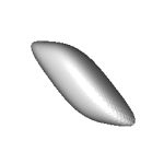
The following Figure 2 and 3 shows the figures of convex bodies that are enclosed by constant surfaces. The number of figures corresponds to that in our list of absolutely nonsingular tensors( Maehara [18]).

Refer to caption
Refer to caption
Refer to caption
Refer to caption
Refer to caption
Refer to caption
Refer to caption
Refer to caption
Figure 2: The constant surfaces for N​o​1,19,22,23,42,60,61,65π‘π‘œ119222342606165No1,19,22,23,42,60,61,65 absolutely nonsingular tensors
Refer to caption
Refer to caption
Refer to caption
Refer to caption
Refer to caption
Refer to caption
Refer to caption
Refer to caption
Figure 3: The constant surfaces for N​o​72,74,76,83,85,87,95,103π‘π‘œ72747683858795103No72,74,76,83,85,87,95,103 absolutely nonsingular tensors

In this section, we want to find some S​L​(3)𝑆𝐿3SL(3)-invariant for such convex bodies. For this purpose, the following valuation theory is a quite useful. Here, we make a brief summary of the valuation theory from Ludwig [15] and [17]. The definition is stated for a general p𝑝p.

Definition 5.1

Let 𝒦𝒦\mathcal{K} denote the set of all convex bodies in ℝpsuperscriptℝ𝑝\mathbb{R}^{p}. A functional t​(β‹…)𝑑⋅t(\cdot) from 𝒦𝒦\mathcal{K} to ℝℝ\mathbb{R} is called a valuation if it satisfies

t​(K)+t​(L)=t​(KβˆͺL)+t​(K∩L),K,Lβˆˆπ’¦.formulae-sequence𝑑𝐾𝑑𝐿𝑑𝐾𝐿𝑑𝐾𝐿𝐾𝐿𝒦t(K)+t(L)=t(K\cup L)+t(K\cap L),\ \ K,L\in\mathcal{K}. (5.2)

Next theorem is a starting point of characterization of invariant valuation.

Theorem 5.3

(Hadwiger[9]). A continuous valuation t​(β‹…)𝑑⋅t(\cdot) from 𝒦𝒦\mathcal{K} to ℝℝ\mathbb{R} is invariant with respect to rigid motion if and only if there are constants c0,c1,…,cpsubscript𝑐0subscript𝑐1…subscript𝑐𝑝c_{0},c_{1},...,c_{p} such that

t​(K)=c0​V0​(K)+c1​V1​(K)+β‹―+cp​Vp​(K),𝑑𝐾subscript𝑐0subscript𝑉0𝐾subscript𝑐1subscript𝑉1𝐾⋯subscript𝑐𝑝subscript𝑉𝑝𝐾t(K)=c_{0}V_{0}(K)+c_{1}V_{1}(K)+\cdots+c_{p}V_{p}(K), (5.4)

where V0​(K),V1​(K),β‹―,subscript𝑉0𝐾subscript𝑉1𝐾⋯V_{0}(K),V_{1}(K),\cdots, and Vp​(K)subscript𝑉𝑝𝐾V_{p}(K) are the intrinsic volumes of K.𝐾K. We remark that the volumes Vksubscriptπ‘‰π‘˜V_{k} are called quermassintegrals of K𝐾K in [13] and that V0subscript𝑉0V_{0} is the Euler index, Vpβˆ’1subscript𝑉𝑝1V_{p-1} the affine volume of βˆ‚K𝐾\partial K, and Vpsubscript𝑉𝑝V_{p} is the volume of the convex body K.𝐾K. In the following, we simply denote by a​(K)π‘ŽπΎa(K) as the affine volume and call it affine surface area following [17], and denoe by V​(K)𝑉𝐾V(K) the volume Vp​(K)subscript𝑉𝑝𝐾V_{p}(K).

Definition 5.5

A functional t​(β‹…)𝑑⋅t(\cdot) on 𝒦𝒦\mathcal{K} is said to be equi-affine invariant if it is S​L​(p)𝑆𝐿𝑝SL(p)-invariant and location invariant.

The following is essential for us.

Theorem 5.6

(Ludwig [14] ,[16], [15] and [17] ). An upper semi-continuous valuation t​(K)𝑑𝐾t(K) from 𝒦𝒦\mathcal{K} to ℝℝ\mathbb{R} is equi-affine invariant if and only if there are constants c0,c1,∈Rc_{0},c_{1},\in R and c2β‰₯0subscript𝑐20c_{2}\geq 0 such that

t​(K)=c0​V0​(K)+c1​Vp​(K)+c2​a​(K),𝑑𝐾subscript𝑐0subscript𝑉0𝐾subscript𝑐1subscript𝑉𝑝𝐾subscript𝑐2π‘ŽπΎt(K)=c_{0}V_{0}(K)+c_{1}V_{p}(K)+c_{2}a(K), (5.7)

where a​(K)π‘ŽπΎa(K) denotes the affine surface area.

In short, S​L​(p)𝑆𝐿𝑝SL(p) invariant valuation is only the weighted sum of the Euler index and the volume Vp​(K)subscript𝑉𝑝𝐾V_{p}(K)and the affine surface area a​(K)π‘ŽπΎa(K). This means that

Proposition 5.8

V​(K)𝑉𝐾V(K) and a​(K)π‘ŽπΎa(K) are S​L𝑆𝐿SL-invariants.

So, we adopt the volume V​(K)𝑉𝐾V(K) and the affine surface area a​(K)π‘ŽπΎa(K) as indexes of S​L​(p)𝑆𝐿𝑝SL(p)-equivalence. Further, the next proposition by Lutwak[20] is very useful for us.

Proposition 5.9

When p=3𝑝3p=3,a​(K)π‘ŽπΎa(K)is homogeneous of degree 3/2323/2, that is,

a​(d​K)=d3/2​a​(K),Kβˆˆπ’¦0.formulae-sequenceπ‘Žπ‘‘πΎsuperscript𝑑32π‘ŽπΎπΎsubscript𝒦0a(dK)=d^{3/2}a(K),K\in\mathcal{K}_{0}. (5.10)

5.1 Volume as an S​L​(3)𝑆𝐿3SL(3)-invariant

We are considering the equivalence relation among absolutely nonsingular tensors. As is shown in Theorem 2.7, for such kind of tensors, the constant surfaces of them are compact. Note that from Propisition 5.8 the volume of the region enclosed by the constant surface is S​L​(3)𝑆𝐿3SL(3)-invariant. Then, by the following Gauss’s theorem, we can calculate the volume by the parametric representation given by the equation (2.6).

Theorem 5.11

(Gaussian formula)
For the region ΩΩ\Omega enclosed by the space surface βˆ‚Ξ©Ξ©\partial\Omega, letting f​d​y∧d​z+g​d​z∧d​x+h​d​x∧d​y𝑓𝑑𝑦𝑑𝑧𝑔𝑑𝑧𝑑π‘₯β„Žπ‘‘π‘₯𝑑𝑦fdy\wedge dz+gdz\wedge dx+hdx\wedge dy be the differential form of 2nd degree, it holds

βˆ«βˆ‚Ξ©f​𝑑y∧d​z+g​d​z∧d​x+h​d​x∧d​y=∫Ω(βˆ‚fβˆ‚x+βˆ‚gβˆ‚y+βˆ‚hβˆ‚z)​𝑑x∧d​y∧d​zsubscriptΩ𝑓differential-d𝑦𝑑𝑧𝑔𝑑𝑧𝑑π‘₯β„Žπ‘‘π‘₯𝑑𝑦subscriptΩ𝑓π‘₯π‘”π‘¦β„Žπ‘§differential-dπ‘₯𝑑𝑦𝑑𝑧\int_{\partial\Omega}fdy\wedge dz+gdz\wedge dx+hdx\wedge dy=\int_{\Omega}\left(\frac{\partial f}{\partial x}+\frac{\partial g}{\partial y}+\frac{\partial h}{\partial z}\right)dx\wedge dy\wedge dz (5.12)

We denote by V​(Ξ©)𝑉ΩV(\Omega) the volume of the region ΩΩ\Omega. By this formula, we have

V​(Ξ©)=L​H​So​ft​h​ee​q​u​a​t​i​o​n​(5.12).π‘‰Ξ©πΏπ»π‘†π‘œπ‘“π‘‘β„Žπ‘’π‘’π‘žπ‘’π‘Žπ‘‘π‘–π‘œπ‘›5.12V(\Omega)=LHS\ \ of\ \ the\ \ equation(\ref{Gauss}). (5.13)

For the present case, by use of the spherical coordinates (s,t), the point of the boundary βˆ‚Ξ©Ξ©\partial\Omega is parametrized as 𝒙=r​(s,t)​(Ξ¦x​(s,t),Ξ¦y​(s,t),Ξ¦z​(s,t)).π’™π‘Ÿπ‘ π‘‘subscriptΞ¦π‘₯𝑠𝑑subscriptΦ𝑦𝑠𝑑subscriptΦ𝑧𝑠𝑑\bm{x}=r(s,t)(\Phi_{x}(s,t),\Phi_{y}(s,t),\Phi_{z}(s,t)). Hence, we have

d​y𝑑𝑦\displaystyle dy =\displaystyle= βˆ‚yβˆ‚s​d​s+βˆ‚yβˆ‚t​d​t𝑦𝑠𝑑𝑠𝑦𝑑𝑑𝑑\displaystyle\frac{\partial y}{\partial s}ds+\frac{\partial y}{\partial t}dt
=\displaystyle= ((βˆ’1/4)​d​p/d​sp5/4​Φy+d​Φy/d​sp1/4)​d​s+limit-from14𝑑𝑝𝑑𝑠superscript𝑝54subscriptΦ𝑦𝑑subscriptΦ𝑦𝑑𝑠superscript𝑝14𝑑𝑠\displaystyle\left((-1/4)\frac{dp/ds}{p^{5/4}}\Phi_{y}+\frac{d\Phi_{y}/ds}{p^{1/4}}\right)ds+
((βˆ’1/4)​d​p/d​tp5/4​Φy+Ξ¦y/d​tp1/4)​d​t14𝑑𝑝𝑑𝑑superscript𝑝54subscriptΦ𝑦subscriptΦ𝑦𝑑𝑑superscript𝑝14𝑑𝑑\displaystyle\left((-1/4)\frac{dp/dt}{p^{5/4}}\Phi_{y}+\frac{\Phi_{y}/dt}{p^{1/4}}\right)dt
d​z𝑑𝑧\displaystyle dz =\displaystyle= βˆ‚zβˆ‚s​d​s+βˆ‚zβˆ‚t​d​t,𝑧𝑠𝑑𝑠𝑧𝑑𝑑𝑑\displaystyle\frac{\partial z}{\partial s}ds+\frac{\partial z}{\partial t}dt,
=\displaystyle= ((βˆ’1/4)​d​p/d​sp5/4​Φz+d​Φz/d​sp1/4)​d​s+limit-from14𝑑𝑝𝑑𝑠superscript𝑝54subscriptΦ𝑧𝑑subscriptΦ𝑧𝑑𝑠superscript𝑝14𝑑𝑠\displaystyle\left((-1/4)\frac{dp/ds}{p^{5/4}}\Phi_{z}+\frac{d\Phi_{z}/ds}{p^{1/4}}\right)ds+
((βˆ’1/4)​d​p/d​tp5/4​Φz+Ξ¦z/d​tp1/4)​d​t.14𝑑𝑝𝑑𝑑superscript𝑝54subscriptΦ𝑧subscriptΦ𝑧𝑑𝑑superscript𝑝14𝑑𝑑\displaystyle\left((-1/4)\frac{dp/dt}{p^{5/4}}\Phi_{z}+\frac{\Phi_{z}/dt}{p^{1/4}}\right)dt.

Therefore,

d​y∧d​z𝑑𝑦𝑑𝑧\displaystyle dy\wedge dz =\displaystyle= ((βˆ’1/4)​d​p/d​sp5/4​Φy+d​Φy/d​sp1/4)​((βˆ’1/4)​d​p/d​tp5/4​Φz+Ξ¦z/d​tp1/4)​d​s∧d​t14𝑑𝑝𝑑𝑠superscript𝑝54subscriptΦ𝑦𝑑subscriptΦ𝑦𝑑𝑠superscript𝑝1414𝑑𝑝𝑑𝑑superscript𝑝54subscriptΦ𝑧subscriptΦ𝑧𝑑𝑑superscript𝑝14𝑑𝑠𝑑𝑑\displaystyle\left((-1/4)\frac{dp/ds}{p^{5/4}}\Phi_{y}+\frac{d\Phi_{y}/ds}{p^{1/4}}\right)\left((-1/4)\frac{dp/dt}{p^{5/4}}\Phi_{z}+\frac{\Phi_{z}/dt}{p^{1/4}}\right)ds\wedge dt
βˆ’((βˆ’1/4)​d​p/d​tp5/4​Φy+Ξ¦y/d​tp1/4)​((βˆ’1/4)​d​p/d​sp5/4​Φz+d​Φz/d​sp1/4)​d​s∧d​t.14𝑑𝑝𝑑𝑑superscript𝑝54subscriptΦ𝑦subscriptΦ𝑦𝑑𝑑superscript𝑝1414𝑑𝑝𝑑𝑠superscript𝑝54subscriptΦ𝑧𝑑subscriptΦ𝑧𝑑𝑠superscript𝑝14𝑑𝑠𝑑𝑑\displaystyle-\left((-1/4)\frac{dp/dt}{p^{5/4}}\Phi_{y}+\frac{\Phi_{y}/dt}{p^{1/4}}\right)\left((-1/4)\frac{dp/ds}{p^{5/4}}\Phi_{z}+\frac{d\Phi_{z}/ds}{p^{1/4}}\right)ds\wedge dt.

Similarly,

d​z∧d​x𝑑𝑧𝑑π‘₯\displaystyle dz\wedge dx =\displaystyle= ((βˆ’1/4)​d​p/d​sp5/4​Φz+d​Φz/d​sp1/4)​((βˆ’1/4)​d​p/d​tp5/4​Φx+Ξ¦x/d​tp1/4)​d​s∧d​t14𝑑𝑝𝑑𝑠superscript𝑝54subscriptΦ𝑧𝑑subscriptΦ𝑧𝑑𝑠superscript𝑝1414𝑑𝑝𝑑𝑑superscript𝑝54subscriptΞ¦π‘₯subscriptΞ¦π‘₯𝑑𝑑superscript𝑝14𝑑𝑠𝑑𝑑\displaystyle\left((-1/4)\frac{dp/ds}{p^{5/4}}\Phi_{z}+\frac{d\Phi_{z}/ds}{p^{1/4}}\right)\left((-1/4)\frac{dp/dt}{p^{5/4}}\Phi_{x}+\frac{\Phi_{x}/dt}{p^{1/4}}\right)ds\wedge dt
βˆ’((βˆ’1/4)​d​p/d​tp5/4​Φz+Ξ¦z/d​tp1/4)​((βˆ’1/4)​d​p/d​sp5/4​Φx+d​Φx/d​sp1/4)​d​s∧d​t,14𝑑𝑝𝑑𝑑superscript𝑝54subscriptΦ𝑧subscriptΦ𝑧𝑑𝑑superscript𝑝1414𝑑𝑝𝑑𝑠superscript𝑝54subscriptΞ¦π‘₯𝑑subscriptΞ¦π‘₯𝑑𝑠superscript𝑝14𝑑𝑠𝑑𝑑\displaystyle-\left((-1/4)\frac{dp/dt}{p^{5/4}}\Phi_{z}+\frac{\Phi_{z}/dt}{p^{1/4}}\right)\left((-1/4)\frac{dp/ds}{p^{5/4}}\Phi_{x}+\frac{d\Phi_{x}/ds}{p^{1/4}}\right)ds\wedge dt,

and

d​x∧d​y𝑑π‘₯𝑑𝑦\displaystyle dx\wedge dy =\displaystyle= ((βˆ’1/4)​d​p/d​sp5/4​Φx+d​Φx/d​sp1/4)​((βˆ’1/4)​d​p/d​tp5/4​Φy+Ξ¦y/d​tp1/4)​d​s∧d​t14𝑑𝑝𝑑𝑠superscript𝑝54subscriptΞ¦π‘₯𝑑subscriptΞ¦π‘₯𝑑𝑠superscript𝑝1414𝑑𝑝𝑑𝑑superscript𝑝54subscriptΦ𝑦subscriptΦ𝑦𝑑𝑑superscript𝑝14𝑑𝑠𝑑𝑑\displaystyle\left((-1/4)\frac{dp/ds}{p^{5/4}}\Phi_{x}+\frac{d\Phi_{x}/ds}{p^{1/4}}\right)\left((-1/4)\frac{dp/dt}{p^{5/4}}\Phi_{y}+\frac{\Phi_{y}/dt}{p^{1/4}}\right)ds\wedge dt
βˆ’((βˆ’1/4)​d​p/d​tp5/4​Φx+Ξ¦x/d​tp1/4)​((βˆ’1/4)​d​p/d​sp5/4​Φy+d​Φy/d​sp1/4)​d​s∧d​t.14𝑑𝑝𝑑𝑑superscript𝑝54subscriptΞ¦π‘₯subscriptΞ¦π‘₯𝑑𝑑superscript𝑝1414𝑑𝑝𝑑𝑠superscript𝑝54subscriptΦ𝑦𝑑subscriptΦ𝑦𝑑𝑠superscript𝑝14𝑑𝑠𝑑𝑑\displaystyle-\left((-1/4)\frac{dp/dt}{p^{5/4}}\Phi_{x}+\frac{\Phi_{x}/dt}{p^{1/4}}\right)\left((-1/4)\frac{dp/ds}{p^{5/4}}\Phi_{y}+\frac{d\Phi_{y}/ds}{p^{1/4}}\right)ds\wedge dt.

By using these, we can calculate the volume of the region enclosed by the constant surface of the determinant polynomial. Let T1subscript𝑇1T_{1} and T2subscript𝑇2T_{2} be two nΓ—nΓ—3𝑛𝑛3n\times n\times 3 tensors and let Ξ©isubscriptΩ𝑖\Omega_{i} denote the regions {b​m​x|fTi​(𝒙)≀1}conditional-setπ‘π‘šπ‘₯subscript𝑓subscript𝑇𝑖𝒙1\{\\ bm{x}|f_{T_{i}}(\bm{x})\leq 1\}, which are enclosed by the surfaces of {𝒙|fT1​(𝒙)=1}conditional-set𝒙subscript𝑓subscript𝑇1𝒙1\{\bm{x}|f_{T_{1}}(\bm{x})=1\}. Then, by S​L​(3)𝑆𝐿3SL(3) invariance of volumes, we have

Theorem 5.16

If V1β‰ V2,subscript𝑉1subscript𝑉2V_{1}\neq V_{2}, fT2​(𝐱)β‰ fT1​(𝐱​R)subscript𝑓subscript𝑇2𝐱subscript𝑓subscript𝑇1𝐱𝑅f_{T_{2}}(\bm{x})\neq f_{T_{1}}(\bm{x}R) for any R∈S​L​(3)𝑅𝑆𝐿3R\in SL(3), namely, T1subscript𝑇1T_{1} and T2subscript𝑇2T_{2} are not S​L​(n)Γ—S​L​(n)Γ—S​L​(3)𝑆𝐿𝑛𝑆𝐿𝑛𝑆𝐿3SL(n)\times SL(n)\times SL(3) equivalent.

For G​L𝐺𝐿GL invariance, the next lemma is helpful.

Lemma 5.17

For a determinant polynomial f​(𝐱),𝑓𝐱f(\bm{x}), let V​(c)𝑉𝑐V(c) be the volume of Ξ©c={𝐱|c​f​(𝐱)≀1}.subscriptΩ𝑐conditional-set𝐱𝑐𝑓𝐱1\Omega_{c}=\{\bm{x}|cf(\bm{x})\leq 1\}. Then V​(c)=cβˆ’3/4​V​(1)𝑉𝑐superscript𝑐34𝑉1V(c)=c^{-3/4}V(1) for 4Γ—4Γ—34434\times 4\times 3 case.

Proof  By changing a polynomial f​(𝒙)𝑓𝒙f(\bm{x}) into its constant multiple c​f​(𝒙)𝑐𝑓𝒙cf(\bm{x}), the coordinates 𝒙​(s,t)𝒙𝑠𝑑\bm{x}(s,t) on the constant surface are subject to changes to (1c)1/4​𝒙​(s,t)superscript1𝑐14𝒙𝑠𝑑(\frac{1}{c})^{1/4}\bm{x}(s,t). Hence, the integral

13β€‹βˆ«βˆ‚Ξ©x​𝑑y∧d​z+y​d​z∧d​x+z​d​x∧d​y13subscriptΞ©π‘₯differential-d𝑦𝑑𝑧𝑦𝑑𝑧𝑑π‘₯𝑧𝑑π‘₯𝑑𝑦\frac{1}{3}\int_{\partial\Omega}xdy\wedge dz+ydz\wedge dx+zdx\wedge dy (5.18)

is multiplied by cβˆ’3/4.superscript𝑐34c^{-3/4}. This proves the assertion of Lemma 5.17. Β 

Theorem 5.19

Assume that T1subscript𝑇1T_{1} and T2subscript𝑇2T_{2} be S​L​(3)𝑆𝐿3SL(3) equivalent and therefore that there is a relation between their determinant polynomials,

fT2​(𝒙)=c​fT1​(𝒙​R),subscript𝑓subscript𝑇2𝒙𝑐subscript𝑓subscript𝑇1𝒙𝑅f_{T_{2}}(\bm{x})=cf_{T_{1}}(\bm{x}R), (5.20)

where cβˆˆβ„π‘β„c\in\mathbb{R} and R∈S​L​(3)𝑅𝑆𝐿3R\in SL(3). Let V1​(c)subscript𝑉1𝑐V_{1}(c) and V2​(c)subscript𝑉2𝑐V_{2}(c) denote the volumes of Ξ©c(1)={𝐱|c​fT1​(𝐱)≀1}subscriptsuperscriptΞ©1𝑐conditional-set𝐱𝑐subscript𝑓subscript𝑇1𝐱1\Omega^{(1)}_{c}=\{\bm{x}|cf_{T_{1}}(\bm{x})\leq 1\} and Ξ©c(2)={𝐱|c​fT2​(𝐱)≀1}subscriptsuperscriptΞ©2𝑐conditional-set𝐱𝑐subscript𝑓subscript𝑇2𝐱1\Omega^{(2)}_{c}=\{\bm{x}|cf_{T_{2}}(\bm{x})\leq 1\} respectively. Then, it holds that

c=(V1/V2)4/3.𝑐superscriptsubscript𝑉1subscript𝑉243c=(V_{1}/V_{2})^{4/3}. (5.21)

Proof  The proof is trivial from Lemma 5.17 and omitted. Β 

From Theorem 5.19, we can know the constant c𝑐c in the equation (5.20). In the next section, it will be made clear that this expresson is helpful for establishing G​L​(3)𝐺𝐿3GL(3)-equivalence.

5.2 Affine surface area as an S​L​(3)𝑆𝐿3SL(3)-invariant

In this section, for testing S​L​(3)𝑆𝐿3SL(3)-equivalence, we propose to use the affine surface area, which is an S​L​(3)𝑆𝐿3SL(3)-invariant by Theorem 5.8. When p=3𝑝3p=3, the affine surface area has the following integral expression.

Definition 5.22

For a smooth convex body KβŠ‚β„3𝐾superscriptℝ3K\subset\mathbb{R}^{3}, the affine surface area is given by

a​(K)=βˆ«βˆ‚Kκ​(K,𝒙)14​E​Gβˆ’F2​𝑑s​𝑑t,π‘ŽπΎsubscriptπΎπœ…superscript𝐾𝒙14𝐸𝐺superscript𝐹2differential-d𝑠differential-d𝑑a(K)=\int_{\partial K}\kappa(K,\bm{x})^{\frac{1}{4}}\sqrt{EG-F^{2}}dsdt, (5.23)

where κ​(βˆ‚K,𝐱)πœ…πΎπ±\kappa(\partial K,\bm{x}) is the Gaussian curvature and E,F𝐸𝐹E,F and G𝐺G denote the first fundamental coefficients.

Next, we show that the affine surface area is useful even as a tester of G​L​(3)𝐺𝐿3GL(3)-equivalence. Assume that we know the constant c𝑐c in the relation fT2​(𝒙)=c​fT1​(𝒙​R)subscript𝑓subscript𝑇2𝒙𝑐subscript𝑓subscript𝑇1𝒙𝑅f_{T_{2}}(\bm{x})=cf_{T_{1}}(\bm{x}R) with cβˆˆβ„+𝑐superscriptℝc\in\mathbb{R}^{+} and R∈S​L​(3)𝑅𝑆𝐿3R\in SL(3) by Theorem 5.19. Then,

Ξ©2subscriptΞ©2\displaystyle\Omega_{2} =\displaystyle= {𝒙|fT2​(𝒙)≀1}conditional-set𝒙subscript𝑓subscript𝑇2𝒙1\displaystyle\{\bm{x}|f_{T_{2}}(\bm{x})\leq 1\}
=\displaystyle= {𝒙|c​fT1​(𝒙)≀1}conditional-set𝒙𝑐subscript𝑓subscript𝑇1𝒙1\displaystyle\{\bm{x}|cf_{T_{1}}(\bm{x})\leq 1\}
=\displaystyle= {𝒙|fT1​(c1/4​𝒙)≀1}conditional-set𝒙subscript𝑓subscript𝑇1superscript𝑐14𝒙1\displaystyle\{\bm{x}|f_{T_{1}}(c^{1/4}\bm{x})\leq 1\}
=\displaystyle= cβˆ’1/4​{𝒙|fT1​(𝒙)≀1}superscript𝑐14conditional-set𝒙subscript𝑓subscript𝑇1𝒙1\displaystyle c^{-1/4}\{\bm{x}|f_{T_{1}}(\bm{x})\leq 1\}
=\displaystyle= cβˆ’1/4​Ω1.superscript𝑐14subscriptΞ©1\displaystyle c^{-1/4}\Omega_{1}.

From Proposition 5.9, we have

a​(Ξ©2)=cβˆ’3/8​a​(Ξ©1).π‘ŽsubscriptΞ©2superscript𝑐38π‘ŽsubscriptΞ©1a(\Omega_{2})=c^{-3/8}a(\Omega_{1}). (5.26)

Thus, we have the following.

Theorem 5.27

Let T1subscript𝑇1T_{1} and T2subscript𝑇2T_{2} be absolutely nonsingular tensors. Noting Remark 4.3, by Theorem 5.19, we can obtain the estimate of c∈R+𝑐superscript𝑅c\in R^{+} under the assumption that their determinant polynomials have the relation fT2​(𝐱)=c​fT1​(𝐱​R)subscript𝑓subscript𝑇2𝐱𝑐subscript𝑓subscript𝑇1𝐱𝑅f_{T_{2}}(\bm{x})=cf_{T_{1}}(\bm{x}R) for some unknown constant cβˆˆβ„+𝑐superscriptℝc\in\mathbb{R}^{+} and an unknown matrix R∈S​L​(3).𝑅𝑆𝐿3R\in SL(3). Then, if a​(Ξ©2)β‰ cβˆ’1/8​a​(Ξ©1)π‘ŽsubscriptΞ©2superscript𝑐18π‘ŽsubscriptΞ©1a(\Omega_{2})\neq c^{-1/8}a(\Omega_{1}), T1subscript𝑇1T_{1} and T2subscript𝑇2T_{2} are not G​L​(3)𝐺𝐿3GL(3) equivalent.

By using Theorem 5.17, this is rephrased as

Theorem 5.28

Let T1subscript𝑇1T_{1} and T2subscript𝑇2T_{2} be absolutely nonsingular tensors. Then, if

a​(Ξ©2)β‰ (V​(Ξ©2)V​(Ξ©1))1/2​a​(Ξ©1),π‘ŽsubscriptΞ©2superscript𝑉subscriptΞ©2𝑉subscriptΞ©112π‘ŽsubscriptΞ©1a(\Omega_{2})\neq\left(\frac{V(\Omega_{2})}{V(\Omega_{1})}\right)^{1/2}a(\Omega_{1}), (5.29)

T1subscript𝑇1T_{1} and T2subscript𝑇2T_{2} are not G​L​(3)𝐺𝐿3GL(3)-equivalent, where V​(Ξ©1)𝑉subscriptΞ©1V(\Omega_{1}) and V​(Ξ©2)𝑉subscriptΞ©2V(\Omega_{2}) denote the volume of Ξ©1subscriptΞ©1\Omega_{1} and Ξ©2subscriptΞ©2\Omega_{2} respectively.

6 Integral G​L​(3)𝐺𝐿3GL(3)-invariant

In the latter half of the previous section, we presented a procedure to test a non-G​L​(3)𝐺𝐿3GL(3)-equivalence, however, it is somewhat indirect because we need to estimate the constant c𝑐c before starting the procedure. In this section, we consider a direct method handling non-equivalence by using a generalized affine surface area. That is, we consider the LqsubscriptπΏπ‘žL_{q} affine surface area, which is an extension of the affine surface area and developed by Letwak [20]. Hug [10] gave an equivalent definition. The following is the Hug’ s definition.

Definition 6.1
Lq​a​(K)=βˆ«βˆ‚KΞΊ0​(K,𝒙)qp+q​𝑑σK​(𝒙)subscriptπΏπ‘žπ‘ŽπΎsubscript𝐾subscriptπœ…0superscriptπΎπ’™π‘žπ‘π‘ždifferential-dsubscriptπœŽπΎπ’™L_{q}a(K)=\int_{\partial K}\kappa_{0}(K,\bm{x})^{\frac{q}{p+q}}d\sigma_{K}(\bm{x}) (6.2)

where

ΞΊ0​(K,𝒙)=κ​(K,𝒙)βŸ¨π’™,𝒏​(K,𝒙)⟩p+1.subscriptπœ…0πΎπ’™πœ…πΎπ’™superscript𝒙𝒏𝐾𝒙𝑝1\kappa_{0}(K,\bm{x})=\frac{\kappa(K,\bm{x})}{\langle\bm{x},\bm{n}(K,\bm{x})\rangle^{p+1}}. (6.3)

and d​σK​(𝐱)𝑑subscript𝜎𝐾𝐱d\sigma_{K}(\bm{x}) is called a cone measure defined by

d​σK​(𝒙)=βŸ¨π’™,𝒏​(K,𝒙)βŸ©β€‹d​𝒙,𝑑subscriptπœŽπΎπ’™π’™π’πΎπ’™π‘‘π’™d\sigma_{K}(\bm{x})=\langle\bm{x},\bm{n}(K,\bm{x})\rangle d\bm{x}, (6.4)

and 𝐧​(K,𝐱)𝐧𝐾𝐱\bm{n}(K,\bm{x}) denotes the outer normal at 𝐱𝐱\bm{x} on βˆ‚K.𝐾\partial K.

When q=1π‘ž1q=1, Lq​(K)subscriptπΏπ‘žπΎL_{q}(K) becomes the affine surface area a​(K)π‘ŽπΎa(K), and when q=pπ‘žπ‘q=p, it becomes a classical centro-affine surface area ac​(K)subscriptπ‘Žπ‘πΎa_{c}(K) thta is defined as

ac​(K)=βˆ«βˆ‚KΞΊ0​(K,𝒙)1/2​𝑑σK​(𝒙),subscriptπ‘Žπ‘πΎsubscript𝐾subscriptπœ…0superscript𝐾𝒙12differential-dsubscriptπœŽπΎπ’™a_{c}(K)=\int_{\partial K}\kappa_{0}(K,\bm{x})^{1/2}d\sigma_{K}(\bm{x}), (6.5)

which is known to be G​L​(p)𝐺𝐿𝑝GL(p)-invariant. The characterization of a general G​L​(p)𝐺𝐿𝑝GL(p)-invariant functional is given below.

Theorem 6.6

(Ludwig and Reitzsner [17] ) Let 𝒦0subscript𝒦0\mathcal{K}_{0} be the space of convex bodies that contain the origin in their interiors. An upper semi-continuous functional t​(β‹…)𝑑⋅t(\cdot) from 𝒦0subscript𝒦0\mathcal{K}_{0} to ℝ1superscriptℝ1\mathbb{R}^{1} is G​L​(p)𝐺𝐿𝑝GL(p)-invariant if and only if there are nonengative constants c0subscript𝑐0c_{0} and c1subscript𝑐1c_{1} such that

t​(K)=c0​V0​(K)+c1​ac​(K).𝑑𝐾subscript𝑐0subscript𝑉0𝐾subscript𝑐1subscriptπ‘Žπ‘πΎt(K)=c_{0}V_{0}(K)+c_{1}a_{c}(K). (6.7)

7 Spherical design

According to our experiments, the numerical integrations of the invariants must be accurate at least 2 decimals. So, the caluculations of the invariants are a little bit heavy. In this section, we consider the t-design method as an substitute of the nemerical integrations. The spherical design was initiated by Delsarte et al. [7] and has been studied by several researchers, for example, see Bannai and Bannai [3]. It is defined as follows.

7.1 An overview of spherical design

Definition 7.1

A finite set X𝑋X on the sphere is called t-spherical design if the following equality holds that for any polynomial f​(x,y,z)𝑓π‘₯𝑦𝑧f(x,y,z) with a degree less than or equal to t,𝑑t,

1|S2|β€‹βˆ«S2f​(x,y,z)​𝑑σ=1|X|β€‹βˆ‘(x,y,z)∈Xf​(x,y,z),1superscript𝑆2subscriptsuperscript𝑆2𝑓π‘₯𝑦𝑧differential-d𝜎1𝑋subscriptπ‘₯𝑦𝑧𝑋𝑓π‘₯𝑦𝑧\displaystyle\frac{1}{|S^{2}|}\int_{S^{2}}f(x,y,z)d\sigma=\frac{1}{|X|}\sum_{(x,y,z)\in X}f(x,y,z), (7.2)

where S2superscript𝑆2S^{2} denotes the unit sphere of ℝ3superscriptℝ3\mathbb{R}^{3} and dβ€‹Οƒπ‘‘πœŽd\sigmadenotes the surface element of the sphere and |S2|superscript𝑆2|S^{2}| denotes the surface area of the sphere.

A parametrized integral formula of the equation 7.2 is given by

∫f​(s,t)​sin⁑(s)​𝑑s​𝑑t=4​πNβ€‹βˆ‘i=1Nf​(si,ti),𝑓𝑠𝑑𝑠differential-d𝑠differential-d𝑑4πœ‹π‘superscriptsubscript𝑖1𝑁𝑓subscript𝑠𝑖subscript𝑑𝑖\int f(s,t)\sin(s)dsdt=\frac{4\pi}{N}\sum_{i=1}^{N}f(s_{i},t_{i}), (7.3)

where (si,ti),i=1,2,….,N(s_{i},t_{i}),i=1,2,....,N are the corresponding parameters to the design points in X𝑋X. One point to overcome for our purpose is that we need to integrate some nonlinear functions that are not polynomials and hence we can not use any t-design directly. However, we can rely on the next theorem to solve this point.

Theorem 7.4

Let f​(x,y,z)𝑓π‘₯𝑦𝑧f(x,y,z) be an continuous function over the unit sphere and let Ο΅tsubscriptitalic-ϡ𝑑\epsilon_{t} be a positive number such that

|f​(x,y,z)βˆ’p​(x,y,z)|<Ο΅t𝑓π‘₯𝑦𝑧𝑝π‘₯𝑦𝑧subscriptitalic-ϡ𝑑|f(x,y,z)-p(x,y,z)|<\epsilon_{t}

uniformly for some polynomial p​(x,y,z)𝑝π‘₯𝑦𝑧p(x,y,z) with degree less than or equal to t𝑑t. Then, it holds that

|βˆ«βˆ‚Sf​(x,y,z)​𝑑Sβˆ’4​π​1Nβ€‹βˆ‘i=1Nf​(xi)|<8​π​ϡtsubscript𝑆𝑓π‘₯𝑦𝑧differential-d𝑆4πœ‹1𝑁superscriptsubscript𝑖1𝑁𝑓subscriptπ‘₯𝑖8πœ‹subscriptitalic-ϡ𝑑|\int_{\partial S}f(x,y,z)dS-4\pi\frac{1}{N}\sum_{i=1}^{N}f(x_{i})|<8\pi\epsilon_{t} (7.5)

Proof

|βˆ«βˆ‚Sf​(x,y,z)​𝑑Sβˆ’4​π​1Nβ€‹βˆ‘i=1Nf​(xi)|subscript𝑆𝑓π‘₯𝑦𝑧differential-d𝑆4πœ‹1𝑁superscriptsubscript𝑖1𝑁𝑓subscriptπ‘₯𝑖\displaystyle\left|\int_{\partial S}f(x,y,z)dS-4\pi\frac{1}{N}\sum_{i=1}^{N}f(x_{i})\right|
≀\displaystyle\leq |βˆ«βˆ‚Sf​(x,y,z)​𝑑Sβˆ’4​π​1Nβ€‹βˆ‘i=1Np​(xi)|+|4​π​1Nβ€‹βˆ‘i=1Np​(xi)βˆ’4​π​1Nβ€‹βˆ‘i=1Nf​(xi)|subscript𝑆𝑓π‘₯𝑦𝑧differential-d𝑆4πœ‹1𝑁superscriptsubscript𝑖1𝑁𝑝subscriptπ‘₯𝑖4πœ‹1𝑁superscriptsubscript𝑖1𝑁𝑝subscriptπ‘₯𝑖4πœ‹1𝑁superscriptsubscript𝑖1𝑁𝑓subscriptπ‘₯𝑖\displaystyle\left|\int_{\partial S}f(x,y,z)dS-4\pi\frac{1}{N}\sum_{i=1}^{N}p(x_{i})\right|+\left|4\pi\frac{1}{N}\sum_{i=1}^{N}p(x_{i})-4\pi\frac{1}{N}\sum_{i=1}^{N}f(x_{i})\right|
=\displaystyle= |βˆ«βˆ‚Sf​(x,y,z)​𝑑Sβˆ’βˆ«|βˆ‚Sp​(xi)​𝑑S​|+4​πN|β€‹βˆ‘i=1N|p​(xi)βˆ’f​(xi)||\displaystyle\left|\int_{\partial S}f(x,y,z)dS-\int_{|\partial S}p(x_{i})dS\right|+\frac{4\pi}{N}\left|\sum_{i=1}^{N}|p(x_{i})-f(x_{i})|\right|
≀\displaystyle\leq ∫ϡt​𝑑S+4​π​ϡtsubscriptitalic-ϡ𝑑differential-d𝑆4πœ‹subscriptitalic-ϡ𝑑\displaystyle\int\epsilon_{t}dS+4\pi\epsilon_{t}
=\displaystyle= 8​π​ϡt8πœ‹subscriptitalic-ϡ𝑑\displaystyle 8\pi\epsilon_{t}

Β 

Remark 7.7

By the above theorem, we need not to know the best approximate polynomial concretely in order to obtain an approximate value of the integration, and it is enough to use f​(x,y,z)𝑓π‘₯𝑦𝑧f(x,y,z) itself. Moreover the error of the approximation is bounded from above by the multiple of Ο΅tsubscriptitalic-ϡ𝑑\epsilon_{t} by 8​π.8πœ‹8\pi. For a substantial evaluation of the approximation, we need to know Ο΅tsubscriptitalic-ϡ𝑑\epsilon_{t}. The problem is interesting, however, it is a little bit heavy task at present, and so it is postponed to the future work.

7.2 Calculation of integral invariants by a 20-design

Using the result of the previous subsection, we consider the integration

a​(K)=βˆ«ΞΊβ€‹(s,t)1/4​E​Gβˆ’F2​𝑑s​𝑑t.π‘ŽπΎπœ…superscript𝑠𝑑14𝐸𝐺superscript𝐹2differential-d𝑠differential-d𝑑a(K)=\int\kappa(s,t)^{1/4}\sqrt{EG-F^{2}}dsdt. (7.8)

where s,t𝑠𝑑s,t moves 0<s<Ο€0π‘ πœ‹0<s<\pi,0<t<2​π0𝑑2πœ‹0<t<2\pi. This integration can be thought to be an integration over the unit sphere by

a​(K)π‘ŽπΎ\displaystyle a(K) =\displaystyle= ∫(s,t,)∈[0,Ο€]Γ—[0,2Ο€]κ​(s,t)1/4​E​Gβˆ’F2​𝑑s​𝑑t\displaystyle\int_{(s,t,)\in[0,\pi]\times[0,2\pi]}\kappa(s,t)^{1/4}\sqrt{EG-F^{2}}dsdt
=\displaystyle= ∫(s,t,)∈[0,Ο€]Γ—[0,2Ο€]κ​(s,t)1/4​E​Gβˆ’F2sin⁑s​sin⁑s​d​s​d​t\displaystyle\int_{(s,t,)\in[0,\pi]\times[0,2\pi]}\kappa(s,t)^{1/4}\frac{\sqrt{EG-F^{2}}}{\sin s}\sin sdsdt
=\displaystyle= βˆ«βˆ‚Sκ​(s,t)1/4​E​Gβˆ’F2sin⁑s​𝑑S,subscriptπ‘†πœ…superscript𝑠𝑑14𝐸𝐺superscript𝐹2𝑠differential-d𝑆\displaystyle\int_{\partial S}\kappa(s,t)^{1/4}\frac{\sqrt{EG-F^{2}}}{\sin s}dS,

where d​S=s​i​n​(s)𝑑𝑆𝑠𝑖𝑛𝑠dS=sin(s). Hence,

p​(x,y,z)=κ​(s,t)1/4​E​Gβˆ’F2sin⁑s𝑝π‘₯π‘¦π‘§πœ…superscript𝑠𝑑14𝐸𝐺superscript𝐹2𝑠p(x,y,z)=\kappa(s,t)^{1/4}\frac{\sqrt{EG-F^{2}}}{\sin s} (7.11)

is taken to be a function over the unit sphere and so the integral invariant can be approximated by the right hand side of the equation below.

βˆ«βˆ‚Sκ​(s,t)1/4​E​Gβˆ’F2sin⁑s​𝑑S∼4​πNβ€‹βˆ‘i=1Np​(xi,yi,zi)similar-tosubscriptπ‘†πœ…superscript𝑠𝑑14𝐸𝐺superscript𝐹2𝑠differential-d𝑆4πœ‹π‘superscriptsubscript𝑖1𝑁𝑝subscriptπ‘₯𝑖subscript𝑦𝑖subscript𝑧𝑖\int_{\partial S}\kappa(s,t)^{1/4}\frac{\sqrt{EG-F^{2}}}{\sin s}dS\sim\frac{4\pi}{N}\sum_{i=1}^{N}p(x_{i},y_{i},z_{i}) (7.12)

The values of invariants calculated by the lattice method and the 20-design method will be give in the next section. The 20-design method show very nice approximations in some cases, however, do not show good approximations for other cases. That is, for our integration of invariants, the spherical design method does not give stable values, unfortunately. This might suggest that we need to use design with more higher degree than 20.

8 Effectiveness of the invariants as testers of non-equivalence

In this section, we will show the effectiveness of the numerical values of the invariants as testers of non-equivalence. We numerically calculated the volume V​(Ξ©)𝑉ΩV(\Omega), the affine surface area a​(Ξ©)π‘ŽΞ©a(\Omega)and centro-affine surface area ac​(Ξ©)subscriptπ‘Žπ‘Ξ©a_{c}(\Omega) of the region Ξ©={𝒙|f(𝒙≀1}\Omega=\{\bm{x}|f(\bm{x}\leq 1\} defined by the determinant polynomials fT​(𝒙)subscript𝑓𝑇𝒙f_{T}(\bm{x}). As examples, we calculate them for the 16 tensors which are in 𝒦0subscript𝒦0\mathcal{K}_{0}, whose constant surfaces are figured in Figures 2 and 3 in the section 5. The numerical calculations are performed in two way, that is, by the lattice method and by the t-design method, and they are compared. As for the t-design method, we use the 20-design named des.3.216.20 in [8] which has 216 points. In the tables below, M1-P2-G5, M6-P2-G, M1-P2-G7 and 20-design denote the globally adaptive integration with accuracy of 5 digits, pseudo-Monte Carlo integration, the globally adaptive integration with accuracy of 7 digits by 64 decimal calculation and 20-design method by IEEE754 decimal calculation, respectively. For all calculation were done by Mathematica.

Tensor V0 V1 V2 V3
T001 2.9197794095194 2.9197794099529 2.9197794089308 2.9197794061274
T019 4.0314824331814 4.0314824340674 4.0314824332515 4.0314824319603
T022 3.6306602017309 3.6306602004447 3.6306602054741 3.6306602016552
T023 3.4355628950802 3.4355628819358 3.4355628878857 3.4355628897838
T042 3.7515624235646 3.7515624142272 3.7515624197586 3.7515624152774
T060 2.1440485535226 2.1440485507771 2.1440485551454 2.1440485550215
T061 2.8594583429857 2.8594583441125 2.8594583445567 2.8594583445567
T065 3.1084258968340 3.1084258946417 3.1084258957994 3.1084258984271
T072 4.6861403575076 4.6861403597489 4.6861403542060 4.6861403560079
T074 3.6302252513670 3.6302253269919 3.63022533280632 3.6302253350968
Table 1: Volumes by M1-P2-G7 :T​n𝑇𝑛Tn, where n=001,0019,022,023,042,060,061𝑛0010019022023042060061n=001,0019,022,023,042,060,061, 065,072065072065,072 and 074074074 Each line denoted as T𝑇Tn-0 lists the value of the original tensor and the lines T𝑇Tn-i,i=1,2,…,5𝑖12…5i=1,2,...,5 list the values for the transformed tensors of Tn by a randomly chosen matrix of S​L​(3)𝑆𝐿3SL(3).
Tensor M1-P2-G5 M6-P2-G5 M1-P2-G7 20-design
T001-0 9.961493457 9.962796404 9.961471493 9.90317
T001-1 9.961470358 9.961249135 9.961471489 8.73023
T001-2 9.961471133 9.971266750 9.961471486 9.96328
T001-3 9.961470327 9.959509709 9.961471474 9.79057
T001-4 9.961471186 9.979456186 9.961471478 10.88367
T001-5 9.961474220 9.997180989 9.961471490 10.99278
T019-0 11.560007113 11.560055546 11.560007991 11.87277
T019-1 11.560007742 11.552017302 11.560007993 11.69239
T019-2 11.560008558 11.559866424 11.560007993 11.51344
T019-3 11.560007692 11.501609971 11.560007989 13.36769
T019-4 11.560008494 11.545260017 11.560007991 10.40203
T019-5 11.560001924 11.558176522 11.560007996 11.49393
T022-0 11.020675684 11.024551464 11.020674135 11.05202
T022-1 11.020673831 11.016947424 11.020674138 11.45345
T022-2 11.020676195 11.027525350 11.020674147 11.54386
T022-3 11.020673214 11.016006939 11.020674140 11.07524
T022-4 11.020675399 11.031596952 11.020674133 11.37096
T022-5 11.020674431 11.022431931 11.020674135 10.74089
T023-0 10.771760482 10.773095422 10.771760351 10.73293
T023-1 10.771758801 10.774759865 10.771760349 9.26881
T023-2 10.771759301 10.725843291 10.771760352 10.94587
T023-3 10.771759730 10.766135806 10.771760352 13.23848
T023-4 10.771757516 10.773059224 10.771760350 10.78732
T023-5 10.771759533 10.773749461 10.771760351 10.88149
T042-0 11.136697741 11.136755128 11.136697332 10.99424
T042-1 11.136695637 11.140565725 11.136697314 11.28015
T042-2 11.136699257 11.140835239 11.136697323 11.89052
T042-3 11.136721676 11.203272583 11.136697308 12.13058
T042-4 11.136696147 11.106329119 11.136697270 9.81007
T042-5 11.136697731 11.107102150 11.136697313 13.99432
Table 2: Affine surface area:T​n𝑇𝑛Tn, where n=001,019,022,023𝑛001019022023n=001,019,022,023 and 042042042 Each line denoted as T𝑇Tn-0 lists the value of the original tensor and the lines T𝑇Tn-i,i=1,2,…,5𝑖12…5i=1,2,...,5 list the values for the transformed tensors of Tn by a randomly chosen matrix of S​L​(3)𝑆𝐿3SL(3).
Tensor M1-P2-G5 M6-P2-G5 M1-P2-G7 20-design
T060-0 8.704587985 8.705126156 8.704588101 8.74300
T060-1 8.704590255 8.781085267 8.704588109 8.50058
T060-2 8.704596276 8.705498658 8.704588101 8.73210
T060-3 8.704588380 8.711001740 8.704588104 8.80910
T060-4 8.704586669 8.703029024 8.704587984 8.85973
T060-5 8.704588143 8.705901809 8.704588100 8.56701
T061-0 9.759043314 9.759635865 9.759045706 9.741275
T061-1 9.759036154 9.759076500 9.759045704 9.72403
T061-2 9.759050068 9.748685352 9.759045707 9.56041
T061-3 9.759044653 9.734392909 9.759045710 9.76040
T061-4 9.759058206 9.745677922 9.759045694 10.37056
T061-5 9.759046974 9.755984062 9.759045716 8.72501
T065-0 10.273389075 10.274251947 10.273389369 10.33927
T065-1 10.273387633 10.260497042 10.273389360 10.76367
T065-2 10.273389342 10.277789370 10.273389368 10.26620
T065-3 10.273388029 10.249526640 10.273389366 10.42661
T065-4 10.273389939 10.276245030 10.273389370 10.06295
T065-5 10.273397527 10.279052599 10.273389365 10.33636
T072-0 12.483701912 12.483843205 12.483691274 12.67586
T072-1 12.483689616 12.484388161 12.483691282 12.38965
T072-2 12.483690234 12.481034408 12.483691282 10.30731
T072-3 12.483690116 12.498107747 12.483691264 11.96858
T072-4 12.483698348 12.435166726 12.483691276 11.219584
T072-5 12.483686195 12.508162438 12.483691276 10.183837
T074-0 10.732327625 10.732623087 10.732332110 10.80078
T074-1 10.732332283 10.726775221 10.732332117 10.55820
T074-2 10.732337739 10.734008328 10.732332113 11.20578
T074-3 10.732332889 10.724453313 10.732332112 10.87848
T074-4 10.732331733 10.729148909 10.732332214 10.95073
T074-5 10.732329467 10.727707310 10.732332111 10.57017
Table 3: Affine surface area:T​n𝑇𝑛Tn, where n=060,061,065,072𝑛060061065072n=060,061,065,072 and 074074074 Each line denoted as T𝑇Tn-0 lists the value of the original tensor and the lines T𝑇Tn-i,i=1,2,…,5𝑖12…5i=1,2,...,5 list the values for the transformed tensors of Tn by a randomly chosen matrix of S​L​(3)𝑆𝐿3SL(3).

Table 1 shows that the SL invariance of volumes of the redions enclosed by the constant surface is clealry seen numerically for every absolutely nonsingular chosen tensors. Tables 2 and 3 of the affine surface area show that the affine suraface area is SL invariant and that all relevant tensors are not S​L​(4)Γ—S​L​(4)Γ—S​L​(3)𝑆𝐿4𝑆𝐿4𝑆𝐿3SL(4)\times SL(4)\times SL(3) equivalent mutually. From Theorem 5.28, combining the volume data, we also conclude that they are not G​L𝐺𝐿GL equivalent. This last fact is also derived by a direct usage of the centro-affine surface data which is seen in Table 4 and Table 5.

Tensor M1-P2-G7 M6-P2-G5 M1-P2-G5 20-design
T001-0 11.690150892617500 11.687899476332365 11.687898336789288 11.59968
T001-1 11.751922920525157 11.687898955213611 11.687898343722015 8.421025
T001-2 11.689694693901319 11.687898370365255 11.687898355824357 11.68469
T001-3 11.721355953709315 11.687894829195568 11.687898343333765 11.29880
T001-4 11.692877418652227 11.687897242831659 11.687897875631138 10.59083
T001-5 11.679997753276740 11.687897167430656 11.687898359334835 11.46900
T019-0 11.509733354093680 11.509334536488204 11.509333804897551 11.81248
T019-1 11.472821548199051 11.509332873485376 11.509333807975230 12.65290
T019-2 11.509963231209824 11.509337447098934 11.509333799194381 11.32764
T019-3 11.552527050941017 11.509334159193976 11.509333800434498 11.38444
T019-4 11.495864684062547 11.509335287391230 11.509333801132503 11.37034
T019-5 11.522546264759133 11.509333512497239 11.509333798526679 22.50564
T022-0 11.574282949497377 11.568790730790213 11.568790156808308 11.59771
T022-1 11.570887655990263 11.568785645774059 11.568790144452251 11.63356
T022-2 11.568787229271756 11.568788230429048 11.568790347476747 11.90185
T022-3 11.567926875696718 11.568789765657722 11.568790134358534 11.57677
T022-4 11.597381830882211 11.568789372237021 11.568790132199215 13.39389
T022-5 11.561310960443544 11.568790290463560 11.568790451975676 11.44911
T023-0 11.631078897689606 11.626439742081966 11.626439153758515 11.57877
T023-1 11.619997976153462 11.626439518693340 11.626439146934238 11.39835
T023-2 11.611266008293132 11.626440231360507 11.626439154231153 11.43501
T023-3 11.647477652583963 11.626433368429471 11.626439151521914 13.20628
T023-4 11.607565993095791 11.626439544654837 11.626439154062155 10.72795
T023-5 11.620421522261536 11.626439658214246 11.626439152653352 11.74869
T042-0 11.502624357421948 11.504755263366923 11.504752079092657 11.30545
T042-1 11.507105268508006 11.504753311150279 11.504752086650519 11.07124
T042-2 11.519424921951189 11.504753899401661 11.504752079220612 9.41924
T042-3 11.501095106227783 11.504764044950799 11.504752085646500 12.16150
T042-4 11.530791206130419 11.504752412140897 11.504752073761618 10.11515
T042-5 11.499503647742464 11.504752956532382 11.504752076792938 10.64605
Table 4: Centro-affine surface area:T​n𝑇𝑛Tn, where n=001,019,022,023𝑛001019022023n=001,019,022,023 and 042042042 Each line denoted as T𝑇Tn-0 lists the value of the original tensor and the lines T𝑇Tn-i,i=1,2,…,5𝑖12…5i=1,2,...,5 list the values for the transformed tensors of Tn by a randomly chosen matrix of G​L​(3)𝐺𝐿3GL(3).
Tensor M6-P2-G5 M1-P2-G5 M1-P2-G7 20-design
T060-0 11.989971644000403 11.989476119401702 11.989477685702977 12.05017
T060-1 11.990418566344240 11.989479611584825 11.989477723348062 12.01483
T060-2 11.976852295964006 11.989478648296963 11.989477738864300 11.80414
T060-3 11.994778478025750 11.989477993940143 11.989477740049253 11.64148
T060-4 11.989039776987073 11.989478217916079 11.989477724638414 12.09719
T060-5 12.046738095770048 11.989477160425962 11.989477721024015 12.11083
T061-0 11.519673795399891 11.518135424201142 11.518135117247486 11.48023
T061-1 11.518661618867961 11.518134427948641 11.518135113069415 11.45852
T061-2 11.519323023325257 11.518135433182912 11.518135109619174 11.45517
T061-3 11.517878708284445 11.518130456996306 11.518135109891727 11.66299
T061-4 11.517606307852915 11.518129721219993 11.518135107795112 11.47192
T061-5 11.531441863084249 11.518134741001642 11.518135110921667 10.31802
T065-0 11.660951650838694 11.660077139783777 11.660146606151409 11.77330
T065-1 11.657097464096733 11.660146835636129 11.660146583158155 11.64542
T065-2 11.662671583310311 11.660135616613492 11.660146602669996 11.69570
T065-3 11.657074111599187 11.660148534680922 11.660146593520388 11.58150
T065-4 11.661605706427124 11.660146860738219 11.660146601870989 12.45337
T065-5 11.668831112582931 11.660147254608734 11.660146596730511 11.76209
T072-0 11.545589518947570 11.545142097769179 11.545141226929544 11.76647
T072-1 11.545716622630585 11.545139592226001 11.545141221483210 11.52675
T072-2 11.562200209044268 11.545142319259361 11.545141224116661 8.50885
T072-3 11.575704218963165 11.545144648175810 11.545141226744587 10.30769
T072-4 11.535076590703719 11.545140326506765 11.545141235723655 12.22675
T072-5 11.545910129113601 11.545141536682674 11.545141208615009 11.19618
T074-0 11.116314213623787 11.116088526600165 11.116090556639371 11.20632
T074-1 11.109183432623630 11.116086365050504 11.116090553382580 11.09112
T074-2 11.121063605466493 11.116094135711593 11.116090554260284 9.58706
T074-3 11.090134159234779 11.116089713933696 11.116090550551305 10.19594
T074-4 11.135697898280837 11.116091869446610 11.116090554811293 11.15140
T074-5 11.117481923868303 11.116094503240262 11.116090554606608 11.08749
Table 5: Centro-affine surface area:T​n𝑇𝑛Tn, where n=060,061,065,072𝑛060061065072n=060,061,065,072 and 074074074 Each line denoted as T𝑇Tn-0 lists the value of the original tensor and the lines T𝑇Tn-i,i=1,2,…,5𝑖12…5i=1,2,...,5 list the values for the transformed tensors of Tn by a randomly chosen matrix of G​L​(3)𝐺𝐿3GL(3).

Indeed, Tables 4 and 5 show that the centro-affine surface area is really G​L𝐺𝐿GL invarinat, and that three point decimal accuracy will be sufficient to detect non G​L​(3)𝐺𝐿3GL(3)-equivalence between 4Γ—4Γ—34434\times 4\times 3 absolutely nonsingular tensors, whose elements consists of only -1,0,1. The M1-P2-G7 method seems clearly the best for discriminating the tensors relating to G​L𝐺𝐿GL nonequivalence.

9 Conclusion

We treated the S​L​(4)Γ—S​L​(4)Γ—S​L​(3),𝑆𝐿4𝑆𝐿4𝑆𝐿3SL(4)\times SL(4)\times SL(3), G​L​(4)Γ—G​L​(4)Γ—S​L​(3)𝐺𝐿4𝐺𝐿4𝑆𝐿3GL(4)\times GL(4)\times SL(3) or G​L​(4)Γ—G​L​(4)Γ—G​L​(3)𝐺𝐿4𝐺𝐿4𝐺𝐿3GL(4)\times GL(4)\times GL(3) non-equivalence problem of 4Γ—4Γ—34434\times 4\times 3 absolutely nonsingular tensors. We proposed a method to addres to the problem through the determinant polynomials. Furthermore we proposed to solve the problem by differential geometric S​L​(3)𝑆𝐿3SL(3) or G​L​(3)𝐺𝐿3GL(3) invariant of the constant surface of the determinant polynomials. From the numerical analysis by Mathematica, it was shown that the stable values of invariants are obtainable numerically and also it was shown that the affine surface area and the centro-affine surface area are useful to detect the non-equivalence. This means that the algebraic problem: whether a system of algebraic equations with many variables can have real solutions or not, can be resolved by differential geometric methods. It is a nice link between algebra and differential geometry. Second, we investigated the spherical design method for calculating invariants. At present, we think that the values given by the adaptive lattice methods are more reliable than those given by the spherical design method. In some future work, we expect to extend the result to more higher dimensional tensors and to know why the spherical design method does not give stable values of invariants.

References

  • [1] M.D. Atkinson and S. Lloyd, Bounds on the ranks of some 333-tensors, Linear Algebra and its applications 31 (1980), 19–31.
  • [2] M. D. Atkinson and M. Stephens, On the maximal multiplicative complexity of a family of bilinear forms, Linear Algebra and its applications 27 (1979),1–8.
  • [3] E. Bannai and E. Bannai, A survey of spherical designs and algebraic combinatorics on spheres. Europian J. of Combinatorics,30 (2009),1392–1425.
  • [4] W. Blaschke, Vorlesungen ΓΌber Differential geometrie II, Springer Verlag, Berlin 1923.
  • [5] L. Chen, Yi. Chen and Y. Mei, Classification of multipartite entanglement containing infinitely many kinds of states, Phys. Revs. A 74 (2006), no. 5, 052331, 1–12.
  • [6] P. Comon, J.M.F. ten Berge, L.D. Lathauwer and J. Castaing, Generic and typical ranks of multi-way arrays, Linear Algebra Applications 430 (2009), no. 11-12, 2997–3007.
  • [7] P. Delsarte, J.M. Goethals and J.J Seidel, Spherical codes and designs, Geom. Dedicata 6 (1977), 363–388.
  • [8] R. H. Hardin and Sloane, N.J.A., Spherical Designs
    http://www2.research.att.com/Β njas/sphdesigns/dim3/.
  • [9] H. Hadwiger, Vorlesungen u¨¨𝑒\ddot{u}ber Inhalt, OberflaΒ¨Β¨π‘Ž\ddot{a}she und Isoperimetrie, Springer, Berlin,1957.
  • [10] D. Hug, Contributions to affine surface area, manuscripta mathematics 91 (1996), 283–301.
  • [11] T.G. Kolda and B.W, Bader, Tensor decompositions and applications, SIAM Review 51 (2009), no. 3, pp. 455–500.
  • [12] J.B. Kruskal, Three-way arrays: rank and uniqueness of trilinear decompositions, with application to arithmetic complexity and statistics, Linear Algebra and Appl. 18 (1977), no. 2, 95–138.
  • [13] K. Leichtwess, Affine Geometry of Convex bodies, Johann Ambrosius. Barth Verlag, Heidelberg (1998).
  • [14] M. Ludwig, A characterization of affine length and asymptotic approximation of convex discs, Abh. Math. semin. Univ. Hamb. 69 (1999), 75–78.
  • [15] M. Ludwig, Valuations in the affine geometry of convex bodies, Proceedings of the conference ”Integral geometry and convexity”, Wuhan 2004, World Scientific, Singapore (2006), 49–65.
  • [16] M. Ludwig and M. Reitzner, A characterization of affine surface area, Adv. Math. 147 (1999), 138–172.
  • [17] M. Ludwig and M. Reitzner, A Classification of SL(n) invariant Valuations, Annals of Mathematics (2010), in press.
    preprint, http://sites.google.com/site/monikaludwig/.
  • [18] K. Maehara, A list of absolutely nonsingular tensors with βˆ’1,0,1101-1,0,1 elements for 4Γ—4Γ—34434\times 4\times 3 case. Preprint(2010).
  • [19] K. Nomizu and T. Sasaki, Affine Differential Geometry, Cambridge Univ. Press, Cambridge (1994).
  • [20] E. Lutwak,The Brunn-Minkovski-Firey theory II:Affine and geominimal surface areas, Adv.Math. 118 (1996), 244–294.
  • [21] T. Sakata, T. Sumi and M. Miyazaki, Exceptional tensors with three slices and the positivity of its determinant polynomial, Abstarct book of ISI, (2009),CPM37, Theoretical Statistics, 349.
  • [22] T. Sakata, T. Sumi, M. Miyazaki and K. Maehara, Exceptional tensors of 3 x 4 x4 tensors and Hilbert 17 th problem,Abstract book of Statistics, Probability, Operation Research, Computer Science and allied Areas, (2010), Complex Data Analysis and Modelling, 75–76.
  • [23] T. Sumi, M. Miyazaki, M. and T. Sakata, About the maximal rank of 3-tensors over the real and the complex number field, Ann. Inst. Stat. Math. 62 (2010), 807–822.
  • [24] J.M.F. ten- Berge, The typical rank of tall three-way arrays, Psychometrika 65 (2000), no. 4, 525–532.