An elementary exposition of the Efimov effect

Abstract

Two particles that are just shy of binding may develop an infinite number of shallow bound states when a third particle is added. This counterintuitive effect was first predicted by V. Efimov for identical bosons interacting with a short-range pair-wise potential. The Efimov effect persists for non-identical particles, if at least two of the three bonds are almost bound. The Efimov effect has recently been verified experimentally using ultra-cold atoms. We explain the origin of this effect using elementary quantum mechanics, and summarize the experimental evidence for it.

I Introduction

Consider three identical bosons (or fermions with spin and isospin) that occupy a spatially symmetric $s$-state. Efimov predicted in 1970 that the spectrum obeys a geometrical scaling law, such that the ratio of the successive energy eigenvalues of the system is a constant.efimov This scaling results in an accumulation of states near zero energy, with the size of the system growing larger by a factor of about $22.7$ for identical bosons for every state approaching zero energy. The number of these three-body bound states is infinite when the dimer binding is zero. However, the number of three-body bound states is actually reduced as the two-body interaction is made more attractive. More remarkable is the fact that the Efimov effect is independent of the details of the interaction, for example, whether it is between atoms with a pair-wise van der Waals interaction, or between nuclei with a nuclear force. The effect persists even with unequal masses, as long as two of the three dimer bonds have near-zero binding. These statements will be made more precise in the following.

A rigorous proof of Efimov’s prediction followed in 1972.amado Recently, an analytical solution for three identical bosons exhibiting the Efimov spectrum has been obtained.gogolin Efimov examined the triton and ¹²C (the latter as a bound state of three alpha particles) for manifestations of his prediction. However, for nuclear systems, the interaction between two nucleons cannot be adjusted to yield a two-body zero-energy bound state. Also, the Coulomb potential between protons often restricts the examples for which two of the three participants are loosely bound neutronsmazumdar in the field of a nuclear core. However, for ultra-cold neutral atoms with tunable interaction strengths, these drawbacks are absent. The experimental observation of the Efimov effect was first made by Kraemer et al.kraemer with an optically trapped dilute gas of ¹³³Cs atoms at 10 nK. At such low temperatures, thermal motion does not mask quantum effects. Moreover, the two-body interaction between atoms may be fine-tuned using “Feshbach resonance.”fesh ; cohen ; chin Under such conditions, the recombination losses increase sharply due to the formation of Efimov trimers, giving the experimental signature of the effect. More recently, Barontini et al.bar have found evidence for two kinds of Efimov trimers in a mixture of ⁴¹K and ⁸⁷Rb; namely KKRb and KRbRb.

Although there are excellent reviews of Efimov physics (see, for example, Ref. braaten, ), beginning graduate or senior undergraduate students unfamiliar with the quantum three-body problem might find them inaccessible. The Efimov effect arises from the large-distance (asymptotic) behavior of the inverse square interaction. The spectrum resulting from such a potential is well-known,coon ; griffiths ; rajeev and its implications for Efimov physics are discussed in Ref. braaten, .

The main goal of this article is to derive, using elementary quantum mechanics, the effective inverse square interaction in coordinate space of the three-body system. To achieve this goal, we use the separable form of two-body potential, for which the algebra is tractable. The Efimov effect is universal and does not depend on this special choice of a separable potential. A choice of the more familiar local form for the potential would entail more advanced aspects of the three-body problem, while not adding to the essential physics. Our hope is that this article can be used as the basis for introducing the fascinating Efimov effect in an advanced undergraduate, or first year graduate course in quantum mechanics.

The outline of our paper is as follows. In Sec. II we briefly review the low-energy scattering of two particles.pat The rationale for utilizing a nonlocal separable two-body potential near a resonance for the analysis of the three-body systemfonseca is introduced at this stage. Short discussions of the separable potential, and Feshbach resonance follow. The relevant properties of the inverse square interaction for an understanding of the Efimov effect are given in Sec. III. Our discussion of the properties of the inverse square interaction sets the stage for the derivation of the Efimov effect in the three-body problem in Sec. IV. Recent experimental evidence for the Efimov effect, which has resulted in a renewed interest in this topic,phys is briefly presented in Sec. V. Our concluding remarks are in Sec. VI.

II The two-body problem

II.1 Low energy parameters

In the elastic scattering of two particles, the initial and the final energies are the same, and only momentum transfer may take place. The scattering amplitude is said to be “on the energy shell.” The scattering cross section and other observables may be described in terms of a phase shift that occurs in each partial wave of the asymptotic (relative) two-body wave function. We assume that the two-body interaction is central, and falls off faster than $r^{-2}$, where $r$ is the distance between the two particles. If three or more particles are involved, the situation is not so simple, even when the particles interact only pair-wise. If a third particle is present near the pair, it might take away some energy in the scattering process. The two-body scattering amplitude is then said to be “off the energy shell,” and depends on the short-distance behavior of the two-body wave function.

The exact description of the three-body problem is given by three coupled integral equations involving the two-body off-the-energy-shell scattering amplitudes.fad The Efimov effect in the three-body problem is remarkable in the sense that its existence is dictated only by the low-energy two-body elastic scattering properties, and not by the off-shell behavior. The Efimov effect arises as long as the two-body interaction between at least two of the pairs is tuned to resonance, regardless of the interaction potential being, for example, local or nonlocal, of zero range or falling off as $r^{-6}$. At resonance, the two-body wave function is just about bound, and extends over a large distance. The tuning of the two-body interaction to resonance is all-important in giving rise to the Efimov effect.

In this paper we choose a specific form of a nonlocal potential, called a separable potential, that gives an analytical form for the two-body wave function, and for which the treatment of the three-body Faddeev equations is simpler.amado In the example of the three-body problem that we discuss in Sec. IV, we avoid solving the Faddeev equations explicitly, while still obtaining the Efimov spectrum.

For two-body scattering at very low energies, the interaction is effective only in the relative $s$-state, because the centrifugal barrier in the higher partial waves suppresses the particles from coming close together. The $s$-wave scattering amplitude is well-known to be given by

$$f_{0}(k)=\frac{1}{k}\exp(i\delta_{0}(k))\sin\delta_{0}(k)=(k\cot\delta_{0}(k)-ik)^{-1},$$ (1)

where $\delta_{0}(k)$ is the $s$-wave phase shift. The differential cross-section for $s$-wave scattering is isotropic and is given by $|f_{0}(k)|^{2}$. The scattering between the two particles is well-describedbethe ; blatt at low energies by two shape-independent parameters, the scattering length $a$, and the effective range $r_{0}$, where

$$k\cot\delta_{0}(k)=-\frac{1}{a}+\frac{1}{2}r_{0}k^{2}+\ldots$$ (2)

The effective range $r_{0}$ is a measure of the range of the two-body potential, and the scattering length is the intercept of the asymptotic zero-energy $s$-wave wave function. The reader unfamiliar with this description of the two-body problem should study Fig. 1 and read Ref. pat, , Sec. II A.

Consider a situation where the attractive potential is not strong enough to support a two-body bound state, in which case the sign of the scattering length is negative.pat As the potential is made more attractive, the scattering length becomes more and more negative, and goes to $-\infty$ at resonance (that is, a “bound state” at $E=0$), and then flips to $+\infty$ as the strength of the attractive potential is increased. A further increase in the attractive strength drives the scattering length to smaller positive values (but with $a\gg r_{0}$), resulting in the formation of a dimer.pat For a zero-range potential, only the first term on the right-hand side of Eq. (2) survives, and it follows from Eq. (1) that the scattering amplitude is given by $f_{0}=-(1/a+ik)^{-1}$. If we extrapolate the wave number to complex values $k=i\kappa_{0}$ for a bound state at $k^{2}=-\kappa_{0}^{2}$, we see that the resulting dimer has energy $E_{b}=-\hbar^{2}/Ma^{2}$, where $M$ is the mass of each isolated atom. The corresponding wave function for $r>r_{0}$ is given by

$$\psi_{0}(r)\sim\frac{\exp(-r/a)}{r}.$$ (3)

For $r\ll a$, Eq. (3) reduces to $\psi_{0}\sim(1/r-1/a)$, showing the connection of the intercept to the scattering length.

II.2 Separable two-body potential

A separable potential is a special form of nonlocal interaction which has been extensively used in the three-body problem in nuclear physics.mitra ; tabakin It results in considerable simplification of the Faddeev integral equation, which Amado and Nobleamado exploited to give a rigorous treatment of the Efimov effect. The work of Amado and Noble was further developed in Ref. adhikari, . In the following we give the Schrödinger equation for two particles interacting by a separable interaction, and consider the scattering of a heavy particle of mass $M$ interacting with a light one of mass $m$, with the mass ratio $\rho=M/m$. The relative energy is given by $E_{2}={k^{2}}/{\nu^{\prime}}$, where we have set $\hbar=2m=1$ and $\nu^{\prime}=\rho/(\rho+1)$. For simplicity, we assume $\rho\gg 1$, and take $\nu^{\prime}=1$. The eigenvalue equation (after the center-of-mass has been removed) is

$$(k^{2}-H_{0})|\psi_{k}\rangle=V|\psi_{k}\rangle,$$ (4)

where $H_{0}$ is the kinetic energy operator. In r-space Eq. (4) takes the form (where ${\bf r}$ is the relative coordinate between the two particles)

$$(k^{2}+\nabla^{2})\psi_{k}({\bf r})=\!\int\langle{\bf r}|V|{\bf r^{\prime}}\rangle\psi_{k}({\bf r^{\prime}})\,d^{3}r^{\prime},$$ (5)

and in p-space Eq. (4) becomes

$$(k^{2}-p^{2})\psi_{k}({\bf p})=\!\int\langle{\bf p}|V|{\bf p^{\prime}}\rangle\psi_{k}({\bf p^{\prime}})\,d^{3}p^{\prime}.$$ (6)

A separable potential in Hilbert space may be written as $V=-\lambda|g\rangle\langle g|$, where the negative sign is taken for attraction, and $\lambda>0$ determines the strength of the potential. In the coordinate representation, the attractive separable potential in the $s$-state is given by $\langle{\bf r}|V|{\bf r^{\prime}}\rangle=-\lambda g(r)g(r^{\prime})$, where $g(r)$ is taken to be real. When a bound state is present, the Fourier transform of $g(r)$ is closely related to the bound state wave function. The Schrödinger equation in ${\bf p}$-space for a bound state, $k^{2}=-\kappa_{0}^{2}$, is given by

$$(\kappa_{0}^{2}+p^{2})\psi_{\kappa_{0}}({\bf p})=\lambda g(p)\!\int\!g(p^{\prime})\psi_{\kappa_{0}}({\bf p}^{\prime})d^{3}p^{\prime}.$$ (7)

In Eq. (7),

$$g(p)=\!\int\!\langle{\bf p}|{\bf r}\rangle g(r)d^{3}r=\frac{1}{(2\pi)^{3/2}}\!\int\exp(-i{\bf p}\cdot{\bf r})g(r)d^{3}r.$$ (8)

We may write Eq. (7) as

$$\psi_{\kappa_{0}}(p)=\lambda C_{\kappa_{0}}\frac{g(p)}{(\kappa_{0}^{2}+p^{2})},$$ (9)

where $C_{\kappa_{0}}=\!\int g(p^{\prime})\psi_{\kappa_{0}}(p^{\prime})d^{3}p^{\prime}$ is a nonzero constant. If we multiply both sides of Eq. (9) by $g(p)$, and integrateover $d^{3}p$, we obtain the equation that determines the binding energy $\kappa_{0}^{2}$ for a given potential

$$\lambda\!\int\!\frac{g^{2}(p)}{(\kappa_{0}^{2}+p^{2})}d^{3}p=1.$$ (10)

In the next section, a similar equation for the three-body bound state will be obtained.

For explicit calculations we choose the popular Yamaguchi formyamaguchi $g(p)=(p^{2}+\beta^{2})^{-1}$, giving

$$g(r)=\frac{1}{(2\pi)^{3/2}}\!\int\!\exp(i{\bf p}\cdot{\bf r})g(p)d^{3}p=\sqrt{\frac{\pi}{2}}\frac{\exp(-\beta r)}{r}.$$ (11)

We substitute this choice of $g(p)$ in Eq. (9), and take its Fourier transform. After a little algebra, we find that

$$\psi_{\kappa_{0}}(r)=\lambda C_{\kappa_{0}}\sqrt{\frac{\pi}{2}}\left(\frac{\exp(-\kappa_{0}r)}{r}-\frac{\exp(-\beta r)}{r}\right)$$ (12)

For small binding, $\kappa_{0}$ is only slightly greater than zero. We choose a short range potential, so that $\beta\gg\kappa_{0}$, and asymptotically Eq. (12) becomes the same as Eq. (3) obtained from the zero-range approximation. The universal nature of the Efimov effect is independent of the specific choice of $g(r)$, as long as $g(r)$ is short range.

II.3 Feshbach resonance

The strength of the interaction of a zero-range potential is controlled by the scattering length $a$. For cold-atoms the scattering length may be varied by a magnetic field, making use of the Feshbach resonance.fesh ; cohen ; chin Near a Feshbach resonance, two unbound atoms with relative energy $E$ slightly larger than zero may scatter off each other through a potential. This scattering process is said to occur in the “open channel.” When the same two atoms come close together in a different total spin state, they may encounter a different potential, and form a bound or quasi-bound state at energy $E_{\rm res}>E$. The process leading to the formation of a bound or quasi-bound state is called a “closed” channel. The scattering state at energy $E$ does not exist in the closed channel, because the closed channel requires $E_{\rm res}>E$ to dissociate the atoms. Nevertheless, there may be interchannel coupling through a spin-dependent potential that might cause a virtual transition between the two channels. The two atoms in the open channel have different magnetic moments than when they are in the quasi-bound state, and hence the energy gap between the states may be controlled by the relative Zeeman shifts. As a result, the mixing between the two states is more pronounced when the Zeeman energy gap is reduced. In a single-channel description,cohen the two atoms in the open channel may make a virtual transition to the closed channel state and back, giving an effective single-channel scattering length in the open channel that is inversely proportional to the energy gap, $\Delta E$, between the two states, where $\Delta E=\Delta\mu(B-B_{0})$. Here, $\Delta\mu$ is the difference in magnetic moments of the two-atom system in the two channels, and $B_{0}$ is the magnetic field at which the scattering length diverges (at resonance) and changes sign. When $B$ is very different from the resonance value $B_{0}$, the effect of the coupling is small, and the scattering length reduces to its natural “background” value $a_{\rm bg}$. More details in the context of ultra-cold atoms may be found in Refs. moer, and chin, .

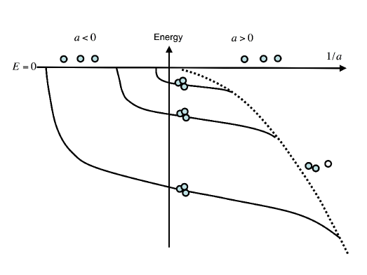
Figure 1: Adapted from Fig. 1 in Ref. phys, . For $a<0$, even though there is no two-body bound state (dimer), more and more three-body bound states (trimers) are formed as the potential becomes more attractive. The solid lines represent these Efimov trimer states which emerge at $E=0$, and $a<0$. For $a>0$ on the right, the trimers break up at the atom-dimer continuum , indicated by the dotted curve

III Efimov spectrum and the Inverse square potential

For three identical bosons interacting pairwise via short-range potentials, Efimov predicted an infinite number of three-body bound states with geometrical scaling, when the two-body interactions are resonant, that is, $|a|\rightarrow\infty$.

Figure 1 (following Ref. phys, ) depicts the Efimov scenario where the energies of some of the three-boson states are plotted as a function of $1/a$; for $E>0$ the energies of the three-atoms form a continuum. The bound Efimov states are shown schematically by solid lines, with a scaling factor (ratio of successive energy eigenvalues) set artificially at 2 rather than $22.7$. The Efimov states break up on the positive side of $a$ in the atom-dimer continuum given by $-\hbar^{2}/(Ma^{2})<E<0$ (see the dotted curve in Fig. 1).

The Efimov spectrum of the three-body problem is the signature of an attractive central potential which falls off asymptotically as the inverse square power of the distance. A three-body long-range potential is suggested by noting that for large positive $a$, the size of the dimer is very large, and the presence of another atom, even if very distant, may be “sensed” by the dimer. For large negative $a$ the two atoms, even if not bound, are spatially correlated over a distance of order $|a|$ in a quasi-bound state.

To obtain the geometric scaling of the spectrum, it is sufficient to consider the simpler problem of a single particle of mass $m$ in an inverse square potential $V(r)=(\hbar^{2}/2m)\lambda/r^{2}$, where $\lambda$ is a dimensionless coupling constant. Classically the equation of motion in this potential is scale invariant under the continuous transformations ${\bf r}\rightarrow\alpha{\bf r}$, and $t\rightarrow\alpha^{2}t$. Quantum mechanically, for $\lambda>-1/4$, there is no bound state, and the continuous scale-invariance is valid. A zero-energy state appears for $\lambda=-1/4$, and the system is anomalous for $\lambda<-1/4$, due to the short-distance singularity of the potential.coon ; griffiths A direct consequence of the anomaly for $\lambda<-1/4$ is that there is no longer a lower limit in the energy spectrum, and a regularization is required.rajeev We are interested in the situation where the potential is inverse square only for $r>r_{c}$, where $r_{c}$ is taken as the short-distance cut-off. We impose the boundary condition that the eigenfunctions vanish at $r=r_{c}$, which results in a discrete spectrum. The geometric scaling property, namely that the ratios of the adjacent energy eigenvalues remain a constant, is independent of $r_{c}$.

We write the Schrödinger equation in the $s$-state for $r>r_{c}$ as

$$\left[-\frac{d^{2}}{dr^{2}}-\frac{(s_{0}^{2}+1/4)}{r^{2}}\right]u(r)=\frac{2m}{\hbar^{2}}Eu(r),$$ (13)

where at this stage, $s_{0}^{2}\geq 0$ is just a way of parametrizing the strength of an inverse square potential that is greater than $1/4$. For bound states, we set $(2m/\hbar^{2})E=-\kappa^{2}$, and require that wave functions vanish at infinity. We then obtain the solution $u(\kappa r)=\sqrt{\kappa r}K_{is_{0}}(\kappa r)$, where $K_{is_{0}}$ is the modified Bessel function of the third kind of pure imaginary order ${is_{0}}$. braaten The boundary condition that $u(\kappa r_{c})=0$ makes $\kappa$ discrete, such that $K_{is_{o}}(\kappa_{n}r_{c})=0$, with $n$ a positive integer. For shallow bound states such that $(\kappa_{n}r_{c}\ll 1)$, the zeros of the Bessel function $K_{is_{0}}(\kappa_{n}r_{c})$ are given by

$$\kappa_{n}r_{c}=\exp\Big{(}\frac{-n\pi}{s_{0}}\Big{)}(2e^{-\gamma})[1+O(s_{0})+\ldots],$$ (14)

where $\gamma$ is Euler’s constant. Equation (14) leads to the desired result

$$\frac{E_{n+1}}{E_{n}}=\exp(-2\pi/s_{0}),\hskip 28.45274ptn=1,2,\ldots\infty$$ (15)

which is the geometric scaling mentioned previously. Note that the actual value of $E_{n}$ scales as $r_{c}^{-2}$, but geometric scaling holds for the shallow states. Also note that as $n$ becomes larger, the states become shallower, with an infinite number of states accumulating at zero energy. In the three-body problem in which three particles interact pair-wise, there are six degrees of freedom after the center-of-mass motion is eliminated. This problem is commonly treated in hyperspherical coordinatesnielsen with a hyperradial variable $R$, and five angles. For equal mass particles,note $R=\sqrt{(r_{12}^{2}+r_{23}^{2}+r_{31}^{2})/3}$. In the adiabatic approximationmacek for fixed $R$, we solve the Schrödinger equation for the angular variables, thus obtaining a complete set of adiabatic eigenvalues $\varepsilon(R)$ and corresponding eigenfunctions. The solution shows that in the resonant limit $a\rightarrow\pm\infty$, neglecting channel coupling, the same inverse square potential as in Eq. (1) appears in hyperspherical coordinates, with $r$ replaced by $R$.

For identical bosons, $\exp(\pi/s_{0})\simeq 22.694$, (that is, $s_{0}\approx 1.00624$) but in general, $s_{0}$ depends on the mass ratios. If $a$ is finite and very large, with $|a|\gg r_{0}$, the inverse square interaction $\varepsilon(R)$ is cut-off at a short distance of the order of $r_{0}$, and at a long distance of the order of $|a|$. The number of shallow bound states is given approximately byfonseca

$$N\simeq\frac{s_{0}}{\pi}\ln\frac{|a|}{r_{0}}.$$ (16)

A simplified derivation of Eq. (16) is given in the Appendix.

IV The three-body model

Our objective of obtaining an inverse square interaction in the three-body problem is best served by taking two identical heavy particles $1$ and $2$, each of mass $M$, and particle $3$ of mass $m\ll M$, as shown in Fig. 2.

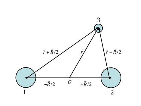
Figure 2: A schematic illustration of the relative coordinates used in the three-body problem. See the text for details.

The coordinates of the particles are labeled ${\bf r}_{1}$, ${\bf r}_{2}$, and ${\bf r}_{3}$, as measured from an arbitrary origin not shown in Fig. 2. The three-body analysis is simplified if the relative coordinates ${\bf R}=({\bf r}_{1}-{\bf r}_{2})$, and ${\bf r}={\bf r}_{3}-({\bf r}_{1}+{\bf r}_{2})/2$ are introduced. Following the common convention, we denote by $V_{1}$ the interparticle potential between particles $2$ and $3$, and likewise for $V_{2}$ and $V_{3}$ in cyclic order. The three-body Schrödinger equation is given by ($\rho=M/m$, and recall that $\hbar=2m=1$)

$$H\Psi({\bf r},{\bf R})=E\Psi({\bf r},{\bf R}),$$ (17)

with

$$H=-\frac{1}{\mu}\nabla^{2}_{R}-\frac{1}{\nu}\nabla^{2}_{r}+V_{1}+V_{2}+V_{3},\quad\mu=\rho/2,\quad\nu=2\rho/(2\rho+1),$$ (18)

where $E$ is the energy of the three-body system. For $\rho\gg 1$, $\nu\rightarrow 1$, and the motion of the heavy particles is very slow compared to that of the light particle of mass $m$, which is in the spirit of the Born-Oppenheimer approximation. Following Ref. fonseca, we may apply the adiabatic Born-Oppenheimer approximation to solve the three-body Schoödinger equation in two stages. First, the wave function is decomposed according to

$$\Psi({\bf r},{\bf R})=\psi({\bf r},{\bf R})\phi({\bf R}),$$ (19)

where $\psi({\bf r},{\bf R})$, with eigenenergy $\varepsilon(R)$, is first solved for the relative motion of the light-heavy system, keeping ${\bf R}$ a parameter. For fixed ${\bf R}$, the relative kinetic energy of the heavy particles is zero, and the potential energy $V_{3}(R)$ is a constant shift in energy. Equation (17), with $\nu=1$, becomes

$$\left[-\nabla_{r}^{2}+V_{1}({\bf r}-{\bf R}/2)+V_{2}({\bf r}+{\bf R}/2)\right]\psi({\bf r},{\bf R})=\varepsilon(R)\psi({\bf r},{\bf R}).$$ (20)

Next, the two-body Schrödinger equation with $\varepsilon(R)$ as the adiabatic potential between the two heavy particles is solved for the ground state energy, $E$, within the adiabatic approximation:

$$\left[-\nabla_{R}^{2}/\mu+V_{3}(R)+\varepsilon(R)\right]\phi(R)=E\phi(R).$$ (21)

Because the interatomic potential $V_{3}(R)$ falls off faster than $1/R^{2}$, it does not affect the asymptotic behavior of $\varepsilon(R)$, and we set $V_{3}(R)=0$. For $V_{1}$ and $V_{2}$ in Eq. (20), we take short-range separable potentials $-\lambda|g\rangle\langle g|$. Thus, for a fixed parameter ${\bf R}$, we have

$$\langle{\bf r}^{\prime}-{\bf R}/2|V_{1}|{\bf r}-{\bf R}/2\rangle=-\lambda\langle{\bf r}^{\prime}-{\bf R}/2|g\rangle\langle g|{\bf r}-{\bf R}/2\rangle,$$ (22)

and likewise for $V_{2}$, with $-{\bf R}/2$ replaced by $+{\bf R}/2$.

If we introduce the displacement operator, $D_{{\bf R}/2}=\exp\left(i{\bf p}_{r}\cdot{\bf R}/2\right)$, we can write $|{\bf r}+{\bf R}/2\rangle=D_{{\bf R}/2}|{\bf r}\rangle$, where ${\bf p}_{r}$ is the momentum conjugate to ${\bf r}$. In operator form, Eq. (20) becomes

$$\left[-\nabla_{r}^{2}-\lambda\left(D|g\rangle\langle g|D^{-1}+D^{-1}|g\rangle\langle g|D\right)\right]|\psi\rangle=\varepsilon(R)|\psi\rangle,$$ (23)

with the subscripts on $D$ suppressed for brevity. Equation (23) bears a striking similarity to the two-body equation in operator notation given by $\left[-\nabla_{r}^{2}-\lambda|g\rangle\langle g|\right]|\psi\rangle=E_{2}|\psi\rangle$. In Eq. (23), let $\varepsilon(R)=-\kappa^{2}(R)$, $G=(-\nabla^{2}_{r}+\kappa^{2})^{-1}$, and $\langle g|D|\psi\rangle=N({\bf R}/2)$. The light-heavy wave function $\psi({\bf r},{\bf R})$ has a definite parity under core-exchange, ${\bf R}\rightarrow-{\bf R}$, so that for the lowest energy state with energy $E$ [recall that we are solving Eq. (21)], we take the wave function to be symmetric. We define $\langle g|D^{-1}|\psi\rangle\equiv N(-{\bf R}/2)=N({\bf R}/2)$, thereby reducing Eq. (23) to

$$|\psi\rangle=\lambda G\left(D^{-1}|g\rangle+D|g\rangle\right)N({\bf R}/2).$$ (24)

We multiply both sides by $\langle g|D$, note that $[G,D]=0$ and $N({\bf R}/2)\neq 0$, and obtain

$$\lambda\left(\frac{\langle g|g\rangle+\langle g|D^{2}|g\rangle}{(-\nabla_{r}^{2}+\kappa^{2})}\right)=1.$$ (25)

In the momentum representation, Eq. (20) takes the form

$$\lambda\!\int\!\frac{g^{2}(p_{r})}{p^{2}_{r}+\kappa^{2}}d^{3}p_{r}+\lambda\!\int\!\frac{g^{2}(p_{r})\exp(i{\bf p_{r}}\cdot{\bf R})}{p^{2}_{r}+\kappa^{2}}d^{3}p_{r}=1,$$ (26)

which is analogous to Eq. (10) for the two-body problem. Note that Eq. (26) assumes $\rho\gg 1$, so that $\nu^{\prime}\simeq\nu$. Recall that $\nu^{\prime}\equiv\rho/(\rho+1)$ and $\nu=2\rho/(2\rho+1)$. The coupling constant $\lambda$ may be eliminated by fixing the binding $\kappa_{0}^{2}$ of the two-body problem. For the Yamaguchi form $g(p)=(p^{2}+\beta^{2})^{-1}$, the integrals in Eq. (26) may be performed analytically, giving

$$1-\left(\frac{\beta+\kappa_{0}}{\beta+\kappa}\right)^{2}=\left(\frac{\beta+\kappa_{0}}{\beta+\kappa}\right)^{2}\left[\frac{2\beta}{(\beta-\kappa)^{2}}\frac{e^{-\kappa R}-e^{-\beta R}}{R}-\frac{\beta+\kappa}{\beta-\kappa}e^{-\beta R}\right].$$ (27)

As the distance $R$ between the two heavy atoms is increased, the light atom will tend to attach to one of them, and $\kappa^{2}(R)\rightarrow\kappa_{0}^{2}$. We are particularly interested in this large $R$ behavior of $\varepsilon(R)$ as the two-body binding $\kappa_{0}^{2}$ goes to zero. To deduce the functional form of $\varepsilon(R)=-\kappa^{2}(R)$ for large $R$, it is convenient to define $\xi\equiv\kappa-\kappa_{0}$, and substitute it into Eq. (27). From Eq. (11), we see that $g(r)$ is short-ranged for $\beta\gg 1$. In the resonant limit, consider $a\rightarrow\infty$ from the positive side. Then $\kappa_{0}=1/a\rightarrow 0$. We consider two possible cases in turn:

(1) $\kappa_{0}\ll\beta$, $\beta R\gg 1$, $R/a\rightarrow 0$, $\xi\ll\beta$ for which $\exp(-\beta R)\rightarrow 0$, and $\exp(-\kappa_{0}R)\rightarrow 1$. Some algebra yields the equation

$$\frac{e^{-\xi R}}{\xi R}=1,$$ (28)

which has the solution $\xi R=A$, where $A=0.5671\ldots$. Hence $\kappa=\kappa_{0}+\xi=\kappa_{0}+A/R$. In the limit of $a\rightarrow\infty$, $\kappa_{0}\rightarrow 0$, we see that $\varepsilon(R)=-\kappa^{2}=-A^{2}/R^{2}$, giving the desired inverse square potential. In our analysis, we set $\nu=1$, which only approximately holds for $\rho\gg 1$. However, setting $\nu=1$ is not necessary, and Fonseca et al.fonseca have shown that $\varepsilon(R)=-A^{2}/(\nu R^{2})$. The effective potential including the kinematic factors that appear in the equation analogous to Eq. (13) may be easily deduced from Eq. (21) to be $-\mu A^{2}/(\nu R^{2})=-1/4A^{2}(1+2\rho)/R^{2}$. Therefore the scaling parameter $s_{0}$ in the Efimov spectrum, as defined in Eq. (13), depends on the mass ratio $\rho$.

(2) Let the scattering length be large but finite, and consider a distance $R$ that is even larger, so that $R/a\gg 1$. $R/a\gg 1$ implies that $\kappa_{0}R\gg 1$, even though the other conditions are the same as in case (1). Thus, in spite of being able to set $\exp(-\beta R)=0$, we cannot set $\exp(-\kappa_{0}R)$ to unity. We may show that for $R\gg a$, Eq. (27) yields the Yukawa form

$$\varepsilon(R)\simeq-\frac{2}{\nu}\frac{e^{-R/a}}{aR}$$ (29)

This form of a static Yukawa potential arises naturally in nuclear physics due to the exchange of a light mass boson (for example, a pion) between two heavy mass nucleons. In nuclear physics the range of the potential is determined by the square root of the mass of the light particle; in our case, it is the square root of the binding energy of the light atom that plays the analogous role. This situation is depicted in Fig. 3. In region I, $R\leq R_{0}$, where $R_{0}$ is the range of the interatomic potentialnewref between the two heavy particles. We cutoff the potential for the shallow states at this distance. In region II there is a $1/R^{2}$ potential, which extends to distances $R\ll a$, hence for all $R$ as $a\rightarrow\infty$, as in case (1). Region III is for $R\sim a$, where the transition to the Yukawa form takes place. Region IV contains the asymptotic behavior of the potential.

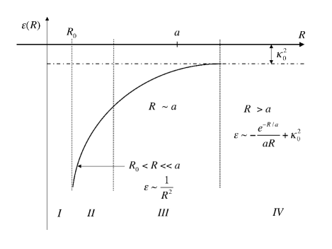
Figure 3: The effective potential $\varepsilon(R)$ between the two heavy-mass particles that arises in the adiabatic approximation due to the interaction with the light-mass particle. For $R<R_{0}$, the interatomic potential is irrelevant for the Efimov effect. The scattering length $a$ is marked on the horizontal axis. As $a\rightarrow\infty$, the two-body binding $\kappa_{0}^{2}$ goes to zero, and $\varepsilon(R)\rightarrow R^{-2}$ for all $R>R_{0}$. The four regions of the potential $\varepsilon(R)$, are discussed in the text.

As the two-body binding $\kappa_{0}^{2}$ goes to zero, the long-range potential $\varepsilon(R)$ takes the inverse square form, which has no length scale. From dimensional considerations, because $\hbar^{2}/M$ has the dimensions of $EL^{2}$, an inverse square potential is the only form possible in the absence of other mass scales or coupling constants.

From Fig. 3, a related prediction associated with the collapse of the three-body system called the Thomas effectthomas may also be deduced. Consider a two-body system of range $r_{0}$ with a fixed binding $\kappa_{0}^{2}$. Let the range parameter $r_{0}$ become smaller and smaller, adjusting the strength of the two-body potential so that $\kappa_{0}^{2}$ remains constant. The Thomas effect asserts that the three-body system will collapse as $r_{0}\rightarrow 0$, with its deepest bound state going to $-\infty$. In Fig. 3, the short distance cut-off $R_{0}$ of the inverse square potential $\varepsilon(R)$ goes to zero as $r_{0}$ goes to zero. Such a behavior near the origin causes a collapse in the three-body energy. The Thomas effect does not require the asymptotic form of the potential to be inverse square, but rather is associated with the short distance singularity of the potential. From Eq. (16) we note that the number of three-body bound states diverges when the ratio $a/r_{0}\rightarrow\infty$, which may be brought about either by letting $a\rightarrow\infty$ with $r_{0}$ finite, as in the Efimov effect, or letting $r_{0}\rightarrow 0$, with $a$ finite, which corresponds to the Thomas effect.fred Unlike the Efimov effect, the Thomas effect is not amenable to experimental verification because the range of the two-body potential cannot, as of now, be tuned to zero.

V Experimental Evidence

Starting with the pioneering work of Kraemer et al.kraemer with ultra-cold Cs atoms in 2006, several experimentszacc ; gross ; pollack have confirmed Efimov’s predictions by measuring the three-body recombination losses of atoms through the reaction $A+A+A\rightarrow A_{2}+A$. The experiment with heteronuclear atoms was done by Barontini et al.bar All these experiments require very low temperature $k_{B}T\leq\hbar^{2}/Ma^{2}$ for a very large scattering length $a$ to avoid break up of the dimers. For example, for Cs atoms, $T=10$ nK was required to largely eliminate thermal effects.

The atoms in a gas have a tendency to form lower energy dimers directly for scattering length $a>0$. But two atoms alone cannot form a bound state and preserve momentum and energy at the same time. Dimer formation is possible if a third atom is nearby within a distance of the order $a$. This problem was studied in a gas of identical atoms with number density $n$, while looking at atomic losses in Bose-Einstein condensates.fed Let the number of three-body recombinations per unit volume per unit time be denoted by $\nu_{\rm rec}$, which is proportional to $n^{2}(\sigma v)(na^{3})$. Here $n^{2}(\sigma v)$ is the probability of two atoms being in the interaction volume $(\sigma v)$, where $\sigma$ is the elastic scattering cross section and $v$ is the relative speed between the two atoms. The probability of finding a third atom within a distance $a$ is $na^{3}$. Because $v=\hbar k/m\simeq\hbar/(ma)$, and $\sigma\propto a^{2}$, we obtain

$$\nu_{\rm rec}=C(a)n^{3}\left(\frac{\hbar}{m}a^{4}\right),$$ (30)

where $m$ is the mass of each atom, and $C(a)$ is a dimensionless constant. The variation of $C(a)$ with the scattering length $a$ exhibits the emergence of an Efimov trimer (negative $a$), and its subsequent dissolution to dimer plus atom (positive $a$), see Fig. 1. It has been calculated from theory.fed ; nielsen2 ; esry The recombination length (the ordinate of Fig.4) is defined as $\rho_{3}=(2\sqrt{3}C(a))^{1/4}a$, where the numerical factor is included to take into account the reduced mass of the trimer, and the fact that three atoms are lost for each trimer.

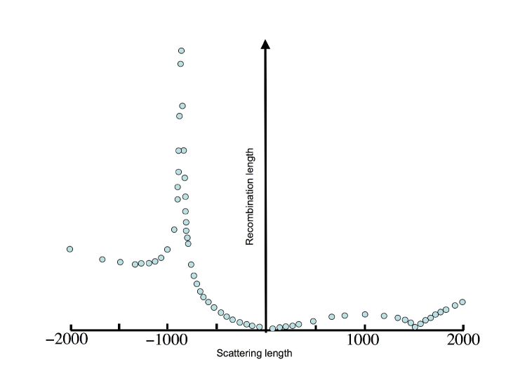
Figure 4: Adapted from Fig. 2 of Ref. esry2, . The solid circles are experimental data points kraemer at $10$ nK for the observed three-body recombination: $Cs+Cs+Cs\rightarrow Cs_{2}+Cs$. The scattering length is measured in units of the Bohr radius $a_{0}$.

To understand the experimental peak in the measured recombination length $\rho_{3}$ (see Fig. 4), note that shallow dimers are not formed directly for $a<0$. The potential $\varepsilon(R)$ of Fig. 3 develops a potential barrier for large $R$, followed by an attractive potential at shorter distances. Such a potential emerges from a hyperspherical calculation for equal mass bosons.macek There may result, for certain negative values of $a$, shape resonances of the trimer at $E>0$. When the energy of the three atoms matches a resonance, there is enhanced barrier penetrability to form an Efimov trimer. The enhanced barrier penetrability allows the system to relax to a deeply bound dimer state (from the interatomic potential), with the excess energy being carried away by the third atom. The peak $\rho_{3}$ on the negative side is at $a=-850a_{0}$, where $a_{0}$ is the Bohr radius. The next peak should be at a value of $a$ that is $22.7$ times larger, that is, $a=-19,295$, which is outside the range of experimental observation. Nevertheless, these multiple peaks were observed in later experiments.zacc ; gross ; pollack Even though multiple resonance peaks were not seen in the Kraemer et al.kraemer experiment, the interference minimum observed on the positive $a$ side is convincing evidence for the Efimov effect.esry2 Hyperspherical calculations for $a>0$ not only give an attractive potential as in Fig. 3 for $\varepsilon(R)$, but also a barrier for positive energies that falls off for large $R$. The three incoming atoms may be reflected by the barrier, and form $A_{2}+A$ on the way out, interfering with the incoming dimer plus atom system following the large-$R$ attractive channel of Fig. 3. The out-of-phase interference between the two paths leads to the curve that fits the experiment for positive $a$ (see Fig. 2 of Ref. esry2, ).

VI Closing remarks

It is remarkable and not foreseeable in 1970 that the Efimov effect has been experimentally verified using ultra-cold atoms. We have considered a simple case for which two of the atoms are very heavy compared to the third. The light heavy pairs are treated very differently, as evidenced by the adiabatic approximation. The light particle is almost unbound, and can be very distant from the heavy partners. The overall size of the shallow Efimov trimer is large in comparison to the short-range of the two-body interaction.

As is clear from Sec. IV, it is the dynamics of the light particle that generates the attractive long-range interaction between the heavy ones. We may regard the light particle as being exchanged back and forth to generate this potential between the two heavy particles. Even for equal mass particles, Efimovcomments has stressed this intuitive picture for the inverse square potential. A different approach must be taken for three identical particles, as indicated briefly in Sec. III for three identical bosons. Each particle has to be treated the same way, and hyperspherical coordinates are well-suited to describe the shallow Efimov states. The size of these states is large, and the small binding results in the formation of floppy triangles. For these shallow states, the coupling between the hyperradial variable $R$ and the hyperangles is small. The coupling vanishes for $|a|\rightarrow\infty$, and the hyperangular contribution just adds a centrifugal term for angular motion to the adiabatic potential $V(R)$. The deepest potential is attractive enough (for $L=0$) to yield the Efimov effect.

For three nucleons the overall wave function under the exchange of any two has to be antisymmetric. As was originally found by Efimov, efimov imposing these symmetries results in only the spatially symmetric angular momentum state $L=0$ (with the spin-isospin combination antisymmetric) leading to an attractive interaction. Unlike charge neutral ultra-cold atoms, it is not possible to manipulate the strength of the nucleon-nucleon interaction.

Given that there is suggestive experimental evidence for the Efimov effect in the four-body sector (see for example, Ref. pollack, ), it is clear that Efimov physics in ultra-cold atoms will continue to be an active area of research.

*

Appendix A Derivation of bound states in the inverse square potential

One way to obtain the number of bound states of a potential is to calculate the canonical partition function $Z(\beta)=\sum_{i}\exp(-\beta E_{i})$, where $\beta$ for our purpose may be taken to be a positive parameter. The expression for $Z(\beta)$ may be written as $Z(\beta)=\!\int_{0}^{\infty}g(E)\exp(-\beta E)dE$, where $g(E)=\sum_{i}\delta(E-E_{i})$ is the density of states. The latter equation shows that $Z(\beta)$ is the Laplace transform of $g(E)$. The inverse Laplace transform of $Z(\beta)$ with respect to $E$ yields the density of states. The integration of the density of states in an energy interval gives the number of states. In the following, we present a simple semiclassical derivation of the number of shallow Efimov states in the energy interval between $0$ and $E$.

Consider the one-body inverse square potential given in Eq. (1)

$$V(r)=-\frac{\hbar^{2}}{2m}\frac{(s_{0}^{2}+1/4)}{r^{2}}.$$ (31)

This form of the potential is taken to be valid for $r_{0}\leq r\leq a$ and for large $a$ (it is assumed that $r_{0}\simeq\tilde{r}$). We shall now derive Eq. (3). The semiclassical partition function for a given partial wave is

$$Z_{\ell}(\beta)=\frac{1}{h}\!\int_{-\infty}^{\infty}dp_{r}\exp(-\beta p_{r}^{2}/2m)\!\int_{0}^{\infty}dr\exp(-\beta V_{\ell}(r)).$$ (32)

After performing the momentum integral in Eq. (32), we obtain

$$Z_{\ell}(\beta)=\left(\frac{m}{2\pi\hbar^{2}}\right)^{1/2}\!\beta^{-1/2}\!\int_{0}^{\infty}e^{-\beta V_{\ell}(r)}dr.$$ (33)

The Laplace inversion of $Z_{\ell}(\beta)$ with respect to $\beta$ gives the density of states

$$g_{\ell}(E)=\left(\frac{m}{2\hbar^{2}}\right)\frac{1}{\pi}\!\int\frac{dr}{\sqrt{E-V_{l}(r)}}\Theta(E-V_{\ell}(r)).$$ (34)

For the inverse square interaction a WKB-type approximation yields exact results when the Langer correction is implemented,guerin that is, $\ell(\ell+1)$ is replaced by $(\ell+1/2)^{2}$. Hence,

$$V_{\ell}(r)=-\frac{\hbar^{2}}{2m}\frac{(s_{0}^{2}+1/4)}{r^{2}}+\frac{\hbar^{2}}{2mr^{2}}(\ell+1/2)^{2}.$$ (35)

We are interested in the $\ell=0$ partial wave, for which

$$V_{0}(r)=-\frac{\hbar^{2}}{2m}\frac{s_{0}^{2}}{r^{2}}.$$ (36)

The number of states is obtained by integrating Eq. (34) with respect to $E$, followed by the integration with respect to $r$:

$$N(E)=\left(\frac{m}{2\hbar^{2}}\right)\frac{2}{\pi}\int_{r_{0}}^{a}\sqrt{E-V_{0}(r)}dr.$$ (37)

If we take $E$ close to zero and $V_{0}(r)$ from Eq. (36, we obtain

$$N\simeq\frac{s_{0}}{\pi}\ln\Big{(}\frac{a}{r_{0}}\Big{)},$$ (38)

which is the well known result for the number of shallow Efimov states.efimov The same derivation applies to the three-body problem with potential $\varepsilon(R)$ (see Fig. 3), when, for very large $a$, we take the form Eq. (31) with $R_{0}\leq R\leq a$.

- (1) V. Efimov, “Energy levels arising from resonant two-body forces in a three-body systems,” Phys. Lett. B 33, 563–564 (1970); “Weakly bound states of three resonantly interacting particles,” Sov. J. Nucl. Phys. 12, 589–595 (1971); “Low-energy properties of three resonantly interacting particles,” Sov. J. Nucl. Phys. 29, 546–453 (1979).
- (2) R. D. Amado and J. V. Noble, “Efimov’s effect: A new pathology of three-particle systems. II,” Phys. Rev. D 5, 1992–2002 (1972).
- (3) A. O. Gogolin, C. Mora, and R. Egger, “Analytical solution of the bosonic three-body problem,” Phys. Rev. Lett. 100, 140404-1–4 (2008).
- (4) I. Mazumdar, A. R. P. Rau, and V. S. Bhasin, “Efimov states and their Fano resonances in a neutron-rich nucleus,” Phys. Rev. Lett. 97, 062503-1–4 (2006).
- (5) T. Kraemer et al., “Evidence for Efimov quantum states in an ultracold gas of caesium atoms,” Nature 440, 315–318 (2006).
- (6) H. Feshbach, “A unified theory of nuclear reactions, II,” Ann. Phys. (NY) 281, 519–546 (2000).
- (7) The reader will find a clear description of the underlying physics of Feshbach resonance in Cohen-Tannoudji’s online lecture-notes “Atom-atom interactions in ultra-cold quantum gases,” Lectures on Quantum Gases, Institut Henri Poincaré, Paris, April 2007. PDF available at http://www.phys.ens.fr/ castin/progtot.html.
- (8) C. Chin, R. Grimm, P. Julienne, and E. Tiesinga, “Feshbach resonance in ultra-cold atoms,” Rev. Mod. Phys. 82, 1225–1286 (2010)
- (9) G. Barontini C. Weber, F. Rabbiti, J. Catani, G. Thalhammer, M. Inguscio, and F. Minardi, “Observation of heteronuclear atomic Efimov resonances,” Phys. Rev. Lett. 103, 043201-1–4 (2009).
- (10) E. Braaten and H.-W. Hammer, “Universality in few-body systems with large scattering length,” Phys. Rep. 428, 259–390 (2006); “Efimov physics in cold atoms,” Ann. Phys. (NY) 322, 120–163 (2007).
- (11) S. A. Coon and B. R. Holstein, “Anomalies in quantum mechanics: The potential,” Am. J. Phys. 70, 513–519 (2002).
- (12) A. M. Essin and D. J. Griffiths, “Quantum mechanics of the potential,” Am. J. Phys. 74, 109–117 (2006).
- (13) K. S. Gupta and S. G. Rajeev, “Renormalization in quantum mechanics,” Phys. Rev. D 48, 5940–5945 (1993).
- (14) P. Shea, B. P. van Zyl, and R. K. Bhaduri, “The two-body problem of ultracold atoms in a harmonic trap,” Am. J. Phys. 77, 511–515 (2009).
- (15) A. Fonseca, E. Redish, and P. E. Shanley, “Efimov effect in an analytically solvable model,” Nucl. Phys. A 320, 273–288 (1979).
- (16) A nontechnical description of recent trends is given by F. Ferlaino and R. Grimm, “Forty years of Efimov physics: How a bizzare prediction turned into a hot topic,” Physics 3, 1–21 (2010); See also C. H. Greene, “Universal insights from few-body land,” Physics Today 53 (3), 40–45 (2010).
- (17) L. D. Faddeev, Mathematical Problems of the Quantum Theory of Scattering for a Three-Particle System (Steklov Mathematical Institute Lelingrad, 1963), No. 69. (English translation by J. B. Sykes (H. M. Stationary Office, Harwell, 1964).
- (18) H. A. Bethe, “Theory of the effective range in nuclear scattering,” Phys. Rev. 76, 38–50 (1949).
- (19) J. M. Blatt and V. F. Weisskopf, Theoretical Nuclear Physics (John Wiley & Sons, NY, 1952), pp. 56–63.
- (20) A. N. Mitra, “Three-body problem with separable potentials,” Nucl. Phys. 32, 521–542 (1961).
- (21) F. Tabakin, “Short-range correlations and the three-body binding energy,” Phys. Rev. 137, B75–B79 (1965).
- (22) S. K. Adhikari, A. C. Fonseca, and L. Tomio, “Method for resonances and virtual states: Efimov’s virtual states,” Phys. Rev. C 26, 77–82 (1982).
- (23) Y. Yamaguchi, “Two-nucleon problem when the potential is nonlocal but separable. I,” Phys. Rev. 95, 1628–1634 1954).
- (24) A. J. Moerdijk, B. J. Verhaar, and A. Axelsson, “ Resonance in ultra-cold collisions of Li and 23Na,” Phys. Rev A 51, 4852–4861 (1995).
- (25) E. Nielsen, D. V. Fedorov, A. S. Jensen, and E. Garrido, “The three-body problem with short-range interactions,” Phys. Rep. 347, 373–459 (2001).
- (26) This definition is taken from Ref. braaten, . Many authors, including Efimovefimov define .
- (27) J. H. Macek, “Efimov states: what are they and why are they important?,” Phys. Scr. 76, C3–C11 (2007).
- (28) In the interatomic problem, the two-body interaction in the relative coordinate is of the van der Waals type, with a tail that falls off as . If we write this part as , it is customary to define the range parameter , where is the reduced mass. See, for example, C. Pethick and H. Smith, Bose-Einstein Condensation of Dilute Gases (Cambridge University Press, Cambridge, 2001).
- (29) L. H. Thomas, “The interaction between a neutron and a proton and the structure of 3H,” Phys. Rev. 47, 903–909 (1935).
- (30) T. Frederico, L. Tomio, A. Delfino, and A. E. A. Amorim, “Scaling limit of weakly bound triatomic states,” Phys. Rev. A 60, R9–R12 (1999).
- (31) M. Zaccanti, B. Deissler, C. D’Errico, M. Fattori , M. Jona-Lasinio, S.Müller, G. Roati, M.Inguscio, and G. Modugno, “Observation of an Efimov spectrum in an atomic system,” Nature Phys. 5, 586–591 (2009).
- (32) N. Gross, Z. Shotan, S. Kokkelmans, and L. Khaykovich, “Observation of universality in ultracold 7Li three-body recombination,” Phys. Rev. Lett. 103, 163202-1–4 (2009).
- (33) S. E. Pollack, D. Dries, and R. G. Hulet, “Universality in three- and four-body bound states of ultracold atoms,” Science 326, 1683–1685 (2009).
- (34) P. O. Fedichev, M. W. Reynolds, and G. V. Shlyapnikov, “Three-body recombinations of ultracold atoms to a weakly bound -level,” Phys. Rev. Lett. 77, 2921–2925 (1996).
- (35) E. Nielsen and J. H. Macek, “Low-energy recombination of identical bosons by three-body collisions,” Phys. Rev. Lett. 83, 1566–1569 (1999).
- (36) B. D. Esry, C. H. Greene, and J. P. Burke Jr., “Recombination of three atoms in the ultracold limit,” Phys. Rev. Lett. 83, 1751–1754 (1999).
- (37) B. D. Esry and C. H. Greene, “A ménage à trois laid bare,” Nature 440, 289–290 (2006).
- (38) V. Efimov, “Is a qualitative approach to the three-body problem useful?,” Comments Nucl. Part. Phys. 19, 271–293 (1990).
- (39) H. Guérin, “Supersymmetric WKB and WKB phase shifts for the Coulomb potential, the inverse-square potential, and their combinations,” J. Phys. B: At. Mol. Opt. Phys. 29, 1285–1291 (1996).