PLEASE PROVIDE
A TITLE by $\backslash$Title{..}

Approximate variances for tapered spectral estimates

Abstract

We propose an approximation of the asymptotic variance that removes a certain discontinuity in the usual formula for the raw and the smoothed periodogram in case a data taper is used. It is based on an approximation of the covariance of the (tapered) periodogram at two arbitrary frequencies. Exact computations of the variances for a Gaussian white noise and an AR(4) process show that the approximation is more accurate than the usual formula.

Key words: Asymptotic variance, data taper, (smoothed) periodogram.

1 Introduction

Spectral estimation is by now a standard topic in time series analysis, and many excellent books are available, e.g. Percival and Walden, (1993) or Bloomfield, (2000). The purpose of this short note is to propose an approximation of the asymptotic variance that removes a certain discontinuity in the usual formula for the raw and the smoothed periodogram in case a taper is used. The standard asymptotic variance of the raw periodogram is independent of the taper chosen, see Formulae (222b) and (223c) in Percival and Walden, (1993). However, this changes when the raw periodogram is smoothed over frequencies close by. Then a variance inflation factor $C_{h}$, see (4), appears which is equal to one if no taper is used and greater than one otherwise, compare Table 248 in Percival and Walden, (1993). The reason for this is that tapering introduces correlations between the raw periodogram at different Fourier frequencies. Because of this, the variance reduction due to smoothing is smaller in the case of no tapering. The above variance inflation factor is justified asymptotically when the number of Fourier frequencies that are involved in the smoothing tends to infinity (more slowly than the number of observations, otherwise we would have a bias). Hence, if only little smoothing is used, then we expect something in between: some increase in the variance, but less than the asymptotic variance inflation factor $C_{h}$. We give here a formula, see (5), which is almost as simple as the inflation factor, but which takes the amount of smoothing into account.

2 Notation and preliminaries

Let $\{X_{t}\}_{t\in\mathbb{Z}}$ be a real-valued stationary process with observation frequency $1/\Delta$, mean $\mathrm{E}[X_{t}]=\mu$, autocovariances $s_{\tau}:=\mathrm{Cov}(X_{t},X_{t+\tau})$ and spectral density $S(f)$. We assume that $X_{1},X_{2},\ldots,X_{N}$ have been observed. The tapered periodogram (called direct spectral estimator in Percival and Walden, (1993)) is

$$\hat{S}^{(tp)}(f):=\frac{\Delta}{\sum_{t=1}^{N}h_{t}^{2}}\left|\sum_{t=1}^{N}h_{t}(X_{t}-\tilde{\mu})e^{-i2\pi itf\Delta}\right|^{2}$$

for $f\in[0,1/(2\Delta)]$. Here the estimator $\tilde{\mu}$ is usually either the arithmetic mean $\bar{X}$ or the weighted average $(\sum_{t=1}^{N}h_{t}X_{t})/(\sum_{t=1}^{N}h_{t}).$ The latter has the property that $\hat{S}^{(tp)}(0)=0$. Since the choice is irrelevant for the asymptotics, we can use either version. The taper $(h_{1},\ldots,h_{N})$ is chosen to reduce the discontinuities of the observation window at the edges $t=1$ and $t=N$. Usually, it has the form $h_{t}=h\left((2t-1)/(2N)\right)$ with a function $h$ that is independent of the sample size $N$. A popular choice is the split cosine taper

$$h^{p}(x)=\left\{\begin{array}[]{ll}\frac{1}{2}(1-\cos(2\pi x/p))&0\leq x\leq\frac{p}{2}\\ 1&\frac{p}{2}<x<1-\frac{p}{2}\\ \frac{1}{2}(1-\cos(2\pi(1-x)/p))&1-\frac{p}{2}\leq x\leq 1\end{array}\right\}.$$ (1)

The tapered periodogram has the approximate variance

$$\mathrm{Var}[\hat{S}^{(tp)}(f)]\approx S(f)^{2},\quad f\notin\{0,1/(2\Delta)\}$$ (2)

(see e.g. Percival and Walden, (1993), Formula (222b)). In particular, it does not converge to zero. Because of this, one usually smoothes the periodogram over a small band of neighboring frequencies. We smooth discretely over an equidistant grid of frequencies. Let $f_{N^{\prime},k}=k/(N^{\prime}\Delta)\ (0\leq k\leq N^{\prime}/2)$ for an integer $N^{\prime}$ of order $O(N)$. Then the tapered and smoothed spectral estimate is

$$\hat{S}^{(ts)}(f_{N^{\prime},k})=\sum_{j=-M}^{M}g_{j}\hat{S}^{(tp)}(f_{N^{\prime},k-j}),$$

where the $g_{j}$’s are weights with the properties $g_{j}>0$, $\ g_{j}=g_{-j}$ $(-M\leq j\leq M)$ and $\sum_{j=-M}^{M}g_{j}=1$. If $k\leq M$, the smoothing includes the value $\hat{S}^{(tp)}(0)$ which is equal or very close to zero if the mean $\mu$ is estimated. In this case, we should exclude $j=k$ from the sum.

3 Approximations of the variance of spectral estimators

The usual approximation for the relative variance of $\hat{S}^{(ts)}(f_{N^{\prime},k})$ is

$$\mathrm{Var}\left(\frac{\hat{S}^{(ts)}(f_{N^{\prime},k})}{S(f_{N^{\prime},k})}\right)\approx C_{h}\frac{N^{\prime}}{N}\sum_{r=-M}^{M}g_{r}^{2}$$ (3)

for $k\neq 0,N^{\prime}/2$ where

$$C_{h}=\frac{\sum_{t=1}^{N}h_{t}^{4}/N}{(\sum_{t=1}^{N}h_{t}^{2}/N)^{2}}.$$ (4)

This formula is given in Bloomfield, (2000), equation (9.12) on p. 183, and it is implemented in the function “spec.pgram” in the language for statistical computing R (R Development Core Team, (2010)). In order to see that it is the same as Formula (248a) in Percival and Walden, (1993), one has to go back to the definition of $W_{m}$ in terms of the weights $g_{j}$ which is given by the formulae (237c), (238d) and (238e). If we put $M=0$, (3) is different from (2). The reason for this difference is that (3) is valid in the limit $M\rightarrow\infty$ and $M/N^{\prime}\rightarrow 0$. But in applications $M$ is often small, e.g. $M=1$, and one wonders how good the approximation is in such a case.

We propose here as alternative the following approximation for the relative variance

$$\left(\sum_{r=-M}^{M}g_{r}^{2}+2\sum_{l=1}^{2M}\frac{\left|H_{2}^{(N)}(f_{N^{\prime},l})\right|^{2}}{H_{2}^{(N)}(0)^{2}}\sum_{r=-M}^{M-l}g_{r}g_{r+l}\right)$$ (5)

(again for $k\neq 0,N^{\prime}/2$) where $H_{2}^{(N)}(f)=\frac{1}{N}\sum_{t=1}^{N}h_{t}^{2}e^{-i2\pi tf\Delta}$. In order to compute this expression, we need to compute the convolution of the weights $(g_{j})$ and the discrete Fourier transform of the squared taper. The former is usually not a problem since $M$ is substantially smaller than $N^{\prime}$. Using the fast Fourier transform, exact computation of the latter is in most cases also possible. If not, then by the Lemma below we can use

$$H_{2}^{(N)}(f)\approx\int_{0}^{1}h^{2}(u)e^{-i2\pi Nuf\Delta}du\ e^{-i\pi f\Delta}\frac{\pi f\Delta}{\sin(\pi f\Delta)}.$$

Choosing a simple form for the function $h$, we can compute the integral on the right exactly. It is obvious that (5) agrees with (2) for $M=0$. In the next section, we show that it also agrees with (3) for $M$ large.

4 Justification of the approximation

The idea is simple: We just plug in a suitable approximation for the relative covariances of the tapered periodogram values into the exact expression for the relative variance. $\mathrm{Var}\left(\hat{S}^{(ts)}(f_{N^{\prime},k})/S(f_{N^{\prime},k})\right)$ is equal to

$$\sum_{r=-M}^{M}\sum_{s=-M}^{M}g_{r}g_{s}\mathrm{Cov}\left(\frac{\hat{S}^{(tp)}(f_{N^{\prime},k-r})}{S(f_{N^{\prime},k-r})},\frac{\hat{S}^{(tp)}(f_{N^{\prime},k-s})}{S(f_{N^{\prime},k-s})}\right).$$ (6)

The asymptotic behavior of these covariances is well known. Theorem 5.2.8 of Brillinger, (1975) shows that, under suitable conditions, we have for frequencies $0<f\leq g<1/(2\Delta)$ that

$$\mathrm{Cov}\left(\frac{\hat{S}^{(tp)}(f)}{S(f)},\frac{\hat{S}^{(tp)}(g)}{S(g)}\right)=\frac{\left|H_{2}^{(N)}(f-g)\right|^{2}+\left|H_{2}^{(N)}(f+g)\right|^{2}}{\left|H_{2}^{(N)}(0)\right|^{2}}+O(N^{-1}).$$ (7)

The statement in Brillinger, (1975) is actually asymmetric in $f$ and $g$ since it has $S(f)$ instead of $S(g)$ on the left side in the equation above. Our statement can be proved by the same argument if we assume $S(f)\approx S(g)$ when $|f-g|$ is small. When $|f-g|$ is big, i.e. not of order $O(N^{-1})$, the covariance is of the order $O(N^{-1})$ anyhow. Using the approximation (7) directly would lead to an approximation which depends on $k$. Having to compute $N^{\prime}/2$ different approximate variances is usually too complicated. However, the term $|H_{2}^{(N)}(f+g)|^{2}$ is small unless $\Delta(f+g)$ is close to zero modulo one. This has been pointed out by Thomson, (1977), see also the discussion on p. 230–231 of Percival and Walden, (1993). If we omit this term, then we obtain our new approximation (5) by a simple change in the summation indices.

We next give a simple lemma that justifies the omission of the second term in (7). In addition, it also shows how the usual approximation (3) follows from (5).

Lemma 4.1.

If $\psi$ is once continuously differentiable on $[0,1]$ and $\psi^{\prime}$ is Lipschitz continuous with constant $L$, then

$$\frac{1}{N}\sum_{t=1}^{N}\psi\left(\frac{2t-1}{2N}\right)e^{-i2\pi\lambda t}=\int_{0}^{1}\psi(u)e^{-i2\pi N\lambda u}du\ e^{-i\pi\lambda}\frac{\pi\lambda}{\sin(\pi\lambda)}+R$$

where $|R|\leq\mathrm{const.}/N$ uniformly for all $\lambda\in[0,0.5]$.

Proof.

Put $\epsilon=1/(2N)$. By a Taylor expansion, we obtain for any $x\in[0,1]$

$$\begin{split}\int_{x-\epsilon}^{x+\epsilon}\psi(u)e^{-i2\pi N\lambda u}du&=\psi(x)e^{-i2\pi N\lambda x}\int_{-\epsilon}^{\epsilon}e^{-i2\pi N\lambda u}du\\ &+\psi^{\prime}(x)e^{-i2\pi N\lambda x}\int_{-\epsilon}^{\epsilon}ue^{-i2\pi N\lambda u}du+R^{\prime}\end{split}$$

where the remainder satisfies $|R^{\prime}|\leq 2\epsilon^{3}L/3=L/(12N^{3}).$ Next, observe that

$$\int_{-\epsilon}^{\epsilon}e^{-i2\pi N\lambda u}du=\frac{\sin(\pi\lambda)}{\pi\lambda N},\ \int_{-\epsilon}^{\epsilon}ue^{-i2\pi N\lambda u}du=\frac{i}{2\pi\lambda N^{2}}\left(\cos(\pi\lambda)-\frac{\sin(\pi\lambda)}{\pi\lambda}\right).$$

From this the lemma follows by taking $x=(2t-1)/(2N)$ for $t=1,\ldots,N$ and summing up all terms. ∎

If $\psi(0)=\psi(1)=0$, then by partial integration

$$\left|\int_{0}^{1}\psi(u)e^{-i2\pi N\lambda u}du\right|\leq\frac{\sup|\psi^{\prime}(x)|}{2\pi\lambda N}.$$

Hence by setting $\psi(u)=h^{2}(u)$, we obtain

$$H_{2}^{(N)}(f)\leq\textrm{const.}(Nf\Delta)^{-1}+\textrm{const.}N^{-1}\leq\mathrm{const.}(Nf\Delta)^{-1}$$ (8)

for $f\leq 1/\Delta$. Therefore the second term in (7) is negligible unless $f+g$ is of the order $O(N^{-1})$.

Finally, we derive the usual variance approximation (3) from (5) as follows. By Parseval’s theorem

$$\sum_{l=-N^{\prime}/2}^{N^{\prime}/2}\left|H_{2}^{(N)}(f_{N^{\prime},l})\right|^{2}=\frac{N^{\prime}}{N}\frac{1}{N}\sum_{t=1}^{N}h_{t}^{4}.$$

Note that $H_{2}^{(N)}(0)=1/N\cdot\sum_{t=1}^{N}h_{t}^{2}$. Because of (8), we have

$$\sum_{l=2M+1}^{N^{\prime}/2}\left|H_{2}^{(N)}(f_{N^{\prime},l})\right|^{2}\leq\sum_{l=2M+1}^{N^{\prime}/2}\left(\frac{\mathrm{const.}\cdot N^{\prime}}{Nl\Delta}\right)^{2}\rightarrow 0$$

for $M\rightarrow\infty$ and $N^{\prime}=O(N)\rightarrow\infty$. Thus

$$\sum_{l=-2M}^{2M}\left|H_{2}^{(N)}(f_{N^{\prime},l})\right|^{2}-\frac{N^{\prime}}{N}\frac{1}{N}\sum_{t=1}^{N}h_{t}^{4}\rightarrow 0,$$

also in the above limit. If the weights $g_{j}$ change smoothly as a function $g$ of the lag $j$, i.e., $g_{j}=g(j/M)$, then for any fixed $l$

$$\sum_{r=-M}^{M-l}g_{r}g_{r+l}\sim M\int_{-1}^{1}g^{2}(u)du\sim\sum_{r=-M}^{M}g_{r}^{2}\ (M\rightarrow\infty)$$

and the desired result follows by dominated convergence.

5 Comparison with exact relative variances for Gaussian processes

If we assume the process $\{X_{t}\}_{t\in\mathbb{Z}}$ to be Gaussian, then it holds

$$\begin{split}&\mathrm{Cov}\left(\frac{\hat{S}^{(tp)}(f)}{S(f)},\frac{\hat{S}^{(tp)}(g)}{S(g)}\right)=\frac{1}{S(f)S(g)(\sum_{t=1}^{N}h_{t}^{2})^{2}}\\ &\times\left(\left|\sum_{j,k=1}^{N}h_{j}h_{k}s_{j-k}e^{-i2\pi(fj-gk)\Delta}\right|^{2}+\left|\sum_{j,k=1}^{N}h_{j}h_{k}s_{j-k}e^{-i2\pi(fj+gk)\Delta}\right|^{2}\right),\end{split}$$

see p. 326 of Percival and Walden, (1993). Plugging this into (6) yields thus an exact expression. Evaluation is of the order $O(N^{3})$, thus it is not practical to use it routinely.

We now compare the two approximations to the exact relative variances for a Gaussian white noise $X_{t}=\epsilon_{t}$ and the AR(4) process

$$X_{t}=2.7607X_{t-1}-3.8106X_{t-2}+2.6535X_{t-3}-0.9238X_{t-4}+\epsilon_{t}$$ (9)

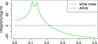
used in Percival and Walden, (1993) (see p. 46) where $\epsilon_{t}\ \mathrm{i.i.d}\sim\mathcal{N}(0,1)$. True spectra are shown in Figure 1 in decibel (dB), i.e., the plot displays $10\log_{10}(S(.))$.

Figure 1: Spectra of the Gaussian white noise and the AR(4) process in (9) in dB.

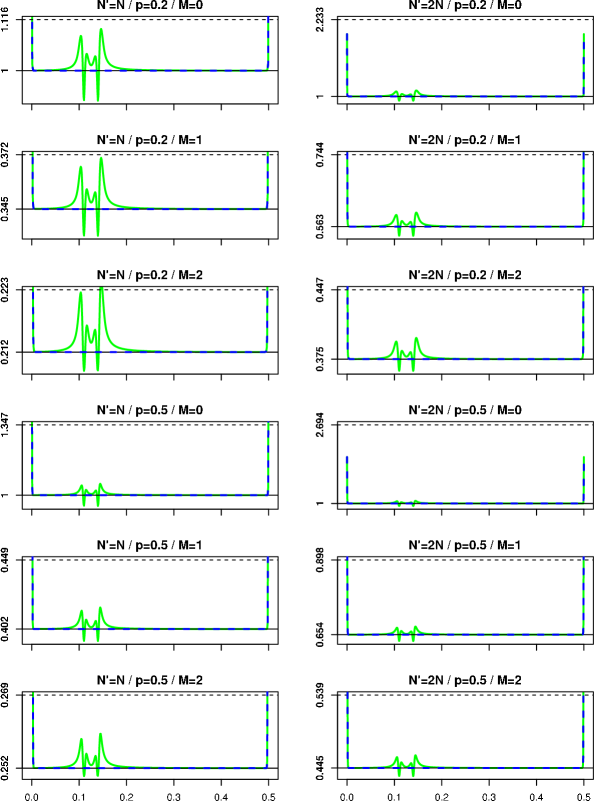
As we can see, the spectrum of the AR(4) process varies over a wide range and exhibits two sharp peaks. Further, we assume the observation frequency $1/\Delta$ to be $1$ and $N=2^{10}=1024$. We compute the exact relative variance (6) at the frequencies $f_{k,N^{\prime}}$, $k=0,\dots,N^{\prime}/2$, for $N^{\prime}\in\{N,2N\}$, the split cosine taper (1) with $p\in\{0.2,0.5\}$ and weights $g_{j}=1/(2M+1)$, $j=-M,\dots,M$, with $M\in\{0,1,2\}$. Comparison to the usual approximation (3) and to the new one (5) is shown in Figure 2. The code in R is available under $\mathbf{http://stat.ethz.ch/\sim kuensch/papers/approximate\_variances.R}$.
We see that the new approximation fits the true relative variances clearly better when we smooth over few frequencies, i.e., $M$ is small. Especially in the situations when the data is strongly tapered ($p=0.5$) or when we use a refined smoothing grid ($N^{\prime}=2N$) we recommend to use the new approximation (5).

Figure 2: Exact relative variances of the Gaussian white noise (thick-dashed) and the AR(4) process (thick-solid) in comparison to the usual (thin-dashed) and the new (thin-solid) approximation for different choices of $N^{\prime}$, $p$ and $M$.

References

• Bloomfield, (2000) Bloomfield, P. (2000). Fourier Analysis of Time Series: An Introduction. Wiley, NY, 2nd edition.
• Brillinger, (1975) Brillinger, D. R. (1975). Time Series, Data Analysis and Theory. International Series in Decision Processes. Holt, Rinehart and Winston, Inc., New York.
• Percival and Walden, (1993) Percival, D. B. and Walden, A. T. (1993). Spectral Analysis for Physical Applications: Multitaper and Conventional Univariate Techniques. Cambridge University Press.
• R Development Core Team, (2010) R Development Core Team (2010). R: A Language and Environment for Statistical Computing. R Foundation for Statistical Computing, Vienna, Austria.
• Thomson, (1977) Thomson, D. J. (1977). Spectrum estimation techniques for characterization and development of WT4 waveguide - I. Bell System Technical Journal, 56:1769–1815.