JM-ECS: A hybrid method combining the $J$-matrix and ECS methods for scattering calculations

Abstract

The paper proposes a hybrid method for calculating scattering processes. It combines the $J$-matrix method with exterior complex scaling and an absorbing boundary condition. The wave function is represented as a finite sum of oscillator eigenstates in the inner region and it is discretized on a grid in the outer region. The method is validated for a one- and two-dimensional model with partial wave equations, and a calculation of $p$-shell nuclear scattering with semi-realistic interactions.

I Introduction

Numerical simulations of breakup reactions are among the most complicated problems in the theoretical physics of nuclear reactions. The main complication arises from the necessity of modeling the asymptotic behavior of the wave function in a many-body continuum. To simplify the asymptotic behavior, the wave function is usually expressed in terms of hyperspherical harmonics Esry et al. (1996); Cobis et al. (1997); Broeckhove et al. (2007). But, in breakup problems, the hyperpotentials decay very slowly and convergence with respect to the hyper-angular momentum is also very slow. This results in very large systems of equations, even for the simplest breakup problems.

The Complex Scaling approach Junker (1982); Moiseyev (1998) can be used to avoid the problems associated with the asymptotic behavior of the many-body wave function. However, this method is suitable only to analyze resonances in the system and it does not provide any breakup information, such as cross sections, that can be compared with experiments.

In the numerical solution of breakup problems described by the Schrödinger equation it is important to describe each of the breakup channels in a correct way. Once the asymptotic form in each of the channels is understood, it is possible to formulate a set of equations whose solution yields both the wave function in the interaction region, and the asymptotic amplitudes in each breakup channel. This is the approach taken both by the $R$-matrix Lane and Thomas (1958) and the $J$-matrix method Heller and Yamani (1974).

However, for some of the breakup channels the asymptotic wave function is only known at very large distance from the target. As a consequence very large numerical domains are needed to cover the interaction and the near-field regions. In other cases, such as the three body breakup in the $J$-matrix representation, the explicit expression of the asymptotic wave function is not known. The need for an explicit asymptotic wave fuction can be avoided by the introduction of absorbing boundary conditions. These enforce an “outgoing wave” boundary condition on the numerical solution, and have been used successfully in atomic and molecular physics McCurdy et al. (2004) and acoustic and electromagnetic scattering problems Berenger (1994). Instead of solving in a single system both the wave function in the interaction region and the reaction rates, these methods calculate the cross section as a post-processing step. First the equations are solved with the absorbing boundary conditions and then, in a second step, the amplitudes are extracted from the numerical solution.

Absorbing boundary conditions are easy to implement in a grid based discretization of a partial differential equation. They have been implemented in calculations based on finite difference, B-splines, finite elements etc McCurdy et al. (2004); Givoli (2008).

In nuclear physics, however, one prefers to use a $L^{2}$-basis, such as the oscillator eigenstates. Such basis is well-adapted to the fully microscopic description of the compound nucleus. This paper reports on the initial efforts to introduce this approach in the context of nuclear few-body systems. We propose a hybrid approach with an $L^{2}$ representation of the wave function in the interaction region, and with a discretized grid representation in the outer region. Our aim is to combine the strengths and benefits of both approaches.

The paper is structured as follows. In section II, after a short review of the ECS and $J$-matrix method, we introduce the hybrid method where the wave function is represented in the inner region by oscillator states and in the outer region by a grid. We also discuss how the observables are extracted from the numerical representation of the scattered wave. In section III we present numerical results that validate the proposed method with model problems for one- and two-dimensional partial wave equations. In section IV we show results for nuclear $p$-shell scattering. We use $m=1$ and $\hbar=1$ throughout the paper, except where mentioned.

II The hybrid $J$-matrix with ECS method

II.1 Exterior Complex Scaling as an outgoing wave boundary condition

Exterior Complex Scaling (ECS) was introduced by B. Simon Simon (1979) and has been initially used for the calculation of resonance positions and widths Moiseyev (1998). It has also found widespread application by providing an absorbing boundary condition in atomic and molecular breakup problems with charged particles Rescigno et al. (1999); Vanroose et al. (2005). A review is given in McCurdy et al. (2004). In these problems the outgoing wave is very complicated, and its form depends on the effective interaction of the outgoing particle. It is determined by the position of the other charged particles involved in the breakup problem.

The derivation of ECS is based on an analytical continuation in the complex plane. It differs from the well-known Complex Scaling (CS) by starting the scaling procedure well into the asymptotic region.

We briefly explain why it leads to outgoing wave boundary conditions and apply these to the Schrödinger equation.

II.1.1 Enforcing outgoing wave boundary conditions

Consider a one-dimensional Helmholtz equation

$$\left(-\frac{d^{2}}{d\rho^{2}}-k^{2}\right)u(\rho)=f(\rho)$$ (1)

on a domain $[0,L]$, with constant wave number $k>0\in\mathbb{R}$, homogeneous Dirichlet conditions on the left boundary, and outgoing wave boundary conditions on the right boundary. The right hand side, $f(\rho)$, is such that it is zero outside the interval $[0,a]$ with $a<L$.

Let us focus this discussion on the right boundary in $L$. For $a<\rho<L$ the equation is a second order homogeneous differential equation with constant coefficients. In this region the general solution can then be written as

$$u(\rho)=Ae^{ik\rho}+Be^{-ik\rho},$$ (2)

a linear combination of two fundamental solutions. Enforcing outgoing wave boundary conditions in $\rho=L$ means that coefficient $B$ should be zero. This can be realized by the following mixed type boundary condition on the solution

$$u^{\prime}(L)=i\,k\,u(L).$$ (3)

Note that this boundary condition requires the explicit knowledge of the wave number $k$.

ECS is an alternative way to enforce the same outgoing wave condition. When we analytically continue the equation (1) to complex $\rho\in\mathbb{C}$, the general solution of the equation, where it is homogeneous, remains a linear combination of the same fundamental modes as in (2). When we impose, instead of the condition (3), a homogeneous Dirichlet boundary condition in the point $L^{\prime}\in\mathbb{C}$ that lies inside the region where the equation is homogeneous, we find that $u(L^{\prime})=0$ leads to $B/A=\exp(2ikL^{\prime})$ or

$$\frac{|B|}{|A|}=\exp(-2\,k\,\mbox{Im}(L^{\prime})).$$ (4)

So if the point $L^{\prime}\in\mathbb{C}$ is chosen such that Im$(L^{\prime})>0$ and $k\,$Im$(L^{\prime})\gg 1$ then $|B|\ll|A|$. As a result, we have, effectively, enforced outgoing wave boundary conditions in the point $L^{\prime}$.

The linear combination of fundamental modes with coefficients $A$ and $B$ describes the solution everywhere where the equation (1) is homogeneous. The equation is homogeneous between the point $L$ and $L^{\prime}$. So the coefficient $B$ of the solution is still much smaller than $A$ in the point $L$ and we can conclude that we also have an outgoing wave boundary condition in $L$.

It is important to note that, in contrast to the mixed boundary condition (3), enforcing Dirichlet boundary conditions in $L^{\prime}$ does not require the knowledge of $k$. This makes it possible to describe both inelastic processes and outgoing boundary conditions in higher dimensions.

II.1.2 ECS contour

We implement this by extending the interval $[0,L]$ with a contour that connects $L$ with $L^{\prime}$. The point $L^{\prime}$ is typically chosen such that $|L|<|L^{\prime}|$ and $k|L^{\prime}|\gg 1$.

Such contour can be formulated as a coordinate transformation on the interval $[0,\,$Re$(L^{\prime})]$.

$$z(\rho)=\left\{\begin{aligned} &\rho&\quad&\text{if}\quad\rho\leq L.\\ &\rho+if(\rho)&\quad&\text{if}\quad L<\rho<\text{Re}(L^{\prime}).\end{aligned}\right.$$ (5)

where $f$ is an increasing function — linear, quadratic, …— with $f(Re(L^{\prime}))=Im(L^{\prime})$ and $f(L)=0$.

In particular, ECS considers a linear function, and the coordinate transformation is therefore written as

$$z(\rho)=\left\{\begin{aligned} &\rho&\quad&\text{for}\quad\rho\leq L.\\ &L+(\rho-L)\mathrm{e}^{\mathrm{i}\theta}&\quad&\text{for}\quad\rho>L.\end{aligned}\right.$$ (6)

II.1.3 Application to the Schrödinger equation

The application of these outgoing wave boundary conditions to the Schrödinger equation is straightforward. Consider, as an example, the two-particle model problem for which the radial equation is

$$(T+V(\rho)+\frac{l(l+1)}{2\rho^{2}}-E)\psi_{sc}(\rho)=-V\hat{j}_{l}(k\rho),$$ (7)

where $T=(-1/2)\,d^{2}/d\rho^{2}$ denotes the kinetic energy operator, $k=\sqrt{2E}$ is the wave number, $l=0,1,2,\ldots$ the angular momentum, $V$ the potential that only depends on the radial coordinate $\rho$, and $\hat{j}_{l}(k\rho)$ the Ricatti-Bessel function, which is the radial part of the incoming wave. The radial solution of this equation is $\psi(\rho)=\hat{j}_{l}(\rho)+\psi_{sc}(\rho)$, a sum of the incoming wave, $\hat{j}_{l}(\rho)$, and the scattered wave, $\psi_{sc}(\rho)$. The latter should fit the outgoing wave boundary conditions.

For problems with short range potentials the Schrödinger equation reduces to the Helmholtz equation outside the range of the potentials with a wave number $k$. We can then apply the ECS transformation in the region where it reduces to a Helmholtz equation.

II.1.4 Discretization

ECS has been implemented in finite differences, B-splines and spectral elements McCurdy et al. (2004). In this section we discretize the differential operator that appears in the Schrödinger equation with finite differences using the Shortley-Weller formula for non-uniform grids Shortley and Weller (1938). It enables the discretization of the operator on the complex contour and uses complex valued mesh widths. Such a mesh mesh is illustrated on Fig. 1

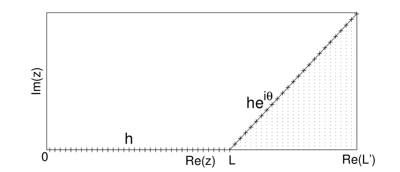
Figure 1: The choice of grid points for the finite difference representation of the Helmholtz equation on a exterior complex scaled (ECS) domain. The original problem was stated on $[0,L]$ with outgoing wave boundary conditions in $L$. The domain is extended with $[L,L^{\prime}]$ where a complex grid distance $h\,e^{i\theta}$ is used. In $L^{\prime}$ homogeneous Dirichlet boundary conditions are enforced.

Consider the differential operator $d^{2}/d{z(\rho)}^{2}$ on the contour defined by the coordinate transformation (6). We define a uniform grid

$$(z_{i})_{0\leq i\leq n}\mbox{ on }[0,L]$$

with $z_{0}=0$ and $z_{n}=L$ and mesh width $h=1/n\in\mathbb{R}$, and a second uniform grid on the complex contour

$$(z_{i})_{n\leq i\leq n+m}\mbox{ on }[L,L^{\prime}]$$

with $z_{n+m}=L^{\prime}$ and complex mesh width $h_{\gamma}=(L^{\prime}-L)/m$. The union of these two grids is the grid

$$(z_{i})_{0\leq i\leq n+m}\mbox{ on }[0,L]\cup[L,L^{\prime}]$$ (8)

in the entire ECS domain. To approximate the second derivative in each grid point $z_{i}$ we use

$$\begin{split}&\frac{d^{2}u(z_{i})}{dz^{2}}\approx\frac{2}{h_{i-1}+h_{i}}\\ &\times\left(\frac{1}{h_{i-1}}u(z_{i-1})-\left(\frac{1}{h_{i-1}}+\frac{1}{h_{i}}\right)u(z_{i})+\frac{1}{h_{i}}u(z_{i+1})\right),\end{split}$$ (9)

where $h_{i-1}$ and $h_{i}$ are the left and right mesh widths respectively, which may be complex valued. The formula reduces to regular second order central differences when $h_{i-1}=h_{i}$, i.e., in the interior real region $[0,L]$, and in the interior of the complex contour $[L,L^{\prime}]$, since the scaling function $f$ is taken to be linear. The only exception is the point $z_{n}$ where we lose at most an order of accuracy. However, with ample discretization steps, the overall accuracy is anticipated to match up to second order. Note that a higher order discretization at the hinge is proposed in Baertschy et al. (2001) to maintain a second order accuracy throughout the domain.

The Hamiltonian of the one-dimensional model (7) is then a $(n+m)$ by $(n+m)$ matrix $\mathsf{H}_{l}\in\mathbb{C}^{n+m}$.

$$\mathsf{H}_{l}=\mathsf{T}+\frac{l(l+1)}{2}\texttt{diag}(1/z_{i}^{2})+\texttt{diag}(V(z_{i})),$$ (10)

where $\mathsf{T}$ is the finite difference representation of the second derivative on the complex contour, and diag is a diagonal matrix with the potential evaluated in each grid point $z_{i}$.

For two-dimensional problems, the Hamiltonian is discretized starting from the one-dimensional discretized Hamiltonian using the Kronecker product $\otimes$

$$\mathsf{H}_{2D}=\mathsf{H}_{l_{1}}\otimes\mathsf{I}+\mathsf{I}\otimes\mathsf{H}_{l_{2}}+\texttt{diag}({V}_{12}(z_{i},z_{j})),$$ (11)

where $\mathsf{I}$ is a $(n+m)$ by $(n+m)$ unit matrix, and diag$(V)$ is the two body potential evaluated at the grid points. The matrix $\mathsf{H}_{2D}$ is now a complex valued $(n+m)^{2}$ by $(n+m)^{2}$ matrix.

The numerical solution of the PDE (7) is found by solving the linear system

$$(\mathsf{H}_{l}-E)\mathsf{x}=\mathsf{b},$$ (12)

where $\mathsf{b}$ is a numerical representation of the right hand side of the equation.

Some examples of one- and two-dimensional wave functions on the ECS domain are presented in Fig. 2 and 3.

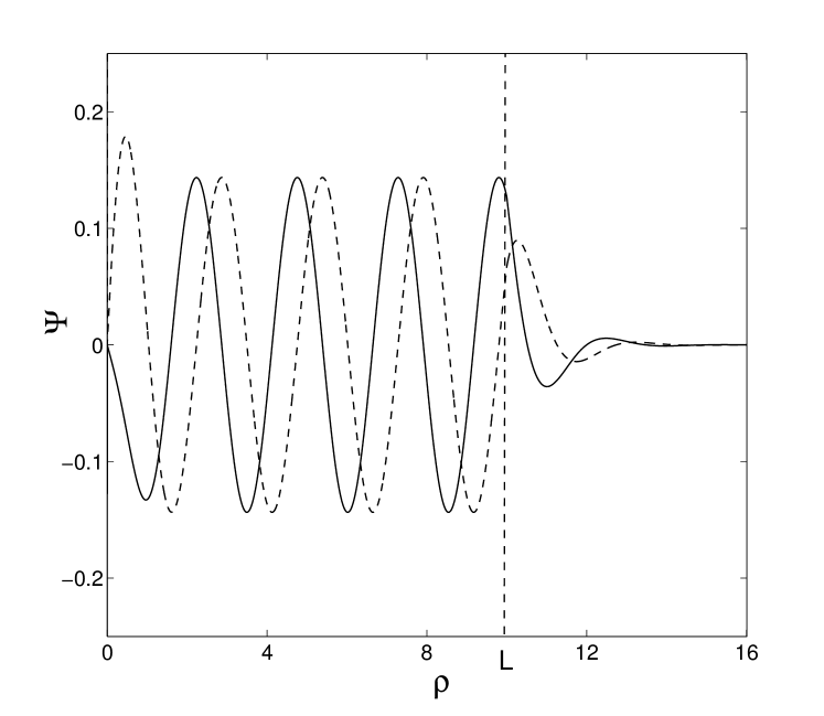
Figure 2: The real and imaginary part of the scattered wave for an Helmholtz problem (1) on the ECS grid. Because of the homogeneous Dirichlet boundary condition the wave is only outgoing in $L$.

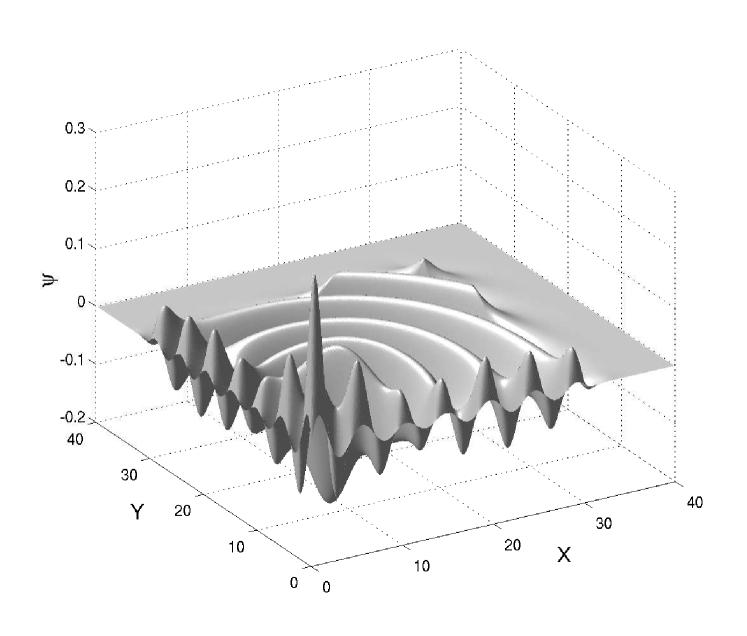
Figure 3: The real part of a 2D partial wave of a three-particle $s$-wave scattering problem on an ECS domain, (49). The problem has a homogeneous Dirichlet boundary condition on the domain $[0,L^{\prime}]^{2}$ and because of the ECS this leads to a problem on the domain $[0,L]^{2}$ with homogeneous Dirichlet boundary condition on the south and west boundary, and outgoing wave boundary conditions on the north and east boundary where $x=L$ or $y=L$. We show the numerical solution of the problem discretized with finite differences.

II.1.5 Extraction of the observables

Once we have the numerical solution of the equation on an ECS domain, we need to extract physical observables such as cross sections.

In one dimension the amplitude $A$ of the outgoing wave can be extracted from the numerical solution with the help of the Wronskian. Indeed, outside the range of the potential $V$ the solution can be written as a linear combination $\psi_{sc}=A\hat{h}_{l}^{+}(kr)+B\hat{h}_{l}^{-}(kr)$, where $\hat{h}_{l}^{\pm}$ are the in- and outgoing Ricatti-Hankel functions. The coefficient $A$ is then

$$A=W\left(\psi_{\text{sc}}(\rho),\hat{h}_{l}^{-}(k\rho)\right)/W\left(\hat{h}_{l}^{+}(k\rho),\hat{h}_{l}^{-}(k\rho)\right),$$ (13)

where $\rho\in[a,L]$ is outside the range of the potential but still on the real part of the ECS domain. The Wronskian is calculated as $W(u,v)=u^{\prime}v-v^{\prime}u$. Since only the values of $\psi_{sc}$ are known on the grid points, its first derivative is approximated by central differences.

In two dimensions the problem is more complicated. The solution inside the numerical box has not reached its far-field form and a projection on the asymptotic state is inaccurate since the single particle and double particle breakup wave functions live in the same regions of space, especial near the edges of the domain. A procedure to extract the observables with the help of surface integrals was proposed by McCurdy, Horner and Rescigno in McCurdy et al. (2001). The amplitude can be written as a surface integral

$$\begin{split}f_{l_{1},l_{2}}(k_{1},f_{2})=&\frac{1}{2}\int_{S}\left(\tau_{k_{1},l_{1}}(\rho_{1})\tau_{k_{2},l_{2}}(\rho_{2})\bm{\nabla}\psi_{sc}(\rho_{1},\rho_{2})\right.\\ &\left.-\psi_{sc}(\rho_{1},\rho_{2})\bm{\nabla}\left(\tau_{k_{1},l_{1}}(\rho_{1})\tau_{k_{2},l_{2}}(\rho_{2})\right)\right)\cdot d\mathbf{S},\end{split}$$ (14)

where $\tau_{k_{1},l_{1}}(\rho_{1})$ is the solution of the radial equation

$$\left(T_{1}+\frac{l_{1}(l_{1}+1)}{2\rho_{1}^{2}}+V_{1}-\frac{k_{1}^{2}}{2}\right)\tau_{k_{1},l_{1}}(\rho)=0.$$ (15)

In a similar way $\tau_{k_{2},l_{2}}(\rho)$ fits the same equation with $T_{2}$, $V_{2}$, $l_{2}$ and $k_{2}^{2}$ such that $k_{1}^{2}+k_{2}^{2}=2E$. The contour of the surface integral, (14), should lie in the region where the Schrödinger equation is homogeneous. In the literature the functions $\tau_{k,l}$ are often denoted as $\phi_{k,l}$. In this paper we have chosen a different notation to avoid confusion with the basis functions of the oscillator representation that will be considered in the next section.

The single differential cross section (SDCS) is then

$$\frac{d\sigma}{dE_{1}}=\frac{8\pi^{2}}{k_{0}^{2}}\frac{1}{k_{1}k_{2}}\left|f(k_{1},k_{2})\right|^{2},$$ (16)

where $k_{0}$ is the momentum of the incoming wave McCurdy et al. (2001).

From these amplitude formulas it is also clear why we use exterior complex scaling rather than complex scaling. In the latter the complete domain is rotated into the complex plane as $\rho\rightarrow\rho e^{i\theta}$ and homogeneous Dirichlet boundary conditions are enforced at the end of the grid. However, after this transformation it is very hard to extract scattering information. In contrast, the sole purpose of ECS is to provide the correct outgoing boundary conditions. It leaves the solution on the real part of the grid unchanged and the scattering cross sections can be extracted.

II.2 The $J$-Matrix Method

In the original $J$-Matrix method for quantum scattering Heller and Yamani (1974, 1974) the wave function is represented in terms of some $L^{2}$-basis set that leads to a tri-diagonal structure of the Hamiltonian matrix for the free-particle problem (Jacobi shape of the matrix). This tri-diagonal structure allows the use of the complete basis set without actually working with matrices of infinite size. A review of the applications of the $J$-matrix method can be found in Alhaidari et al. (2008).

A popular $L^{2}$-basis set for calculations with short-range potentials is the set of eigenstates of the radial harmonic oscillator. The basis states are then generalized Laguerre polynomials multiplied by a weight function

$$\phi_{i,l}(\rho) = (-1)^{i}N_{i,l}b^{-3/2}\left(\frac{\rho}{b}\right)^{l}$$ (17)

$$\times \rho\,\exp\left(-\frac{\rho^{2}}{2b^{2}}\right)L_{i}^{l+1/2}\left(\frac{\rho^{2}}{b^{2}}\right)$$

with a normalization

$$N_{i,l}=\sqrt{\frac{2i!}{\Gamma(i+l+3/2)}},$$ (18)

where $i=0,1,2\ldots$ and oscillator length $b=\sqrt{\hbar/m\omega}$ that is related to the oscillator frequency $\omega$. Note that we have incorporated the weight $\rho$ of integration coming from the radial coordinates in the function (17) such that $\int_{0}^{\infty}\phi_{i,l}(\rho)\phi_{j,l}(\rho)d\rho=\delta_{ij}$

Each basis function has a classical turning point

$$R_{i,l}=b\sqrt{4i+2l+3}.$$ (19)

The oscillator basis set is complete over $L^{2}$ and the solutions of (7) can always be represented as a linear combination of all oscillator states

$$\psi_{l}(\rho)=\sum_{i=0}^{\infty}c_{i,l}\phi_{i,l}(\rho).$$ (20)

This representation reduces the Schrödinger equation to an infinite system of linear equations for $c_{i,l}$.

As already mentioned above, the kinetic energy operator $T$ (the free particle Hamiltonian) is a tri-diagonal matrix in the $J$-matrix method. For the oscillator basis the non-zero elements are

$$J_{i,j}=\left\{\!\!\begin{array}[]{c@{\quad}l}\left(2i+l+\frac{3}{2}\right)\frac{\hbar\omega}{2}&\text{for }j=i,\\ -\sqrt{i\,\left(i+l+\frac{1}{2}\right)}\frac{\hbar\omega}{2}&\text{for }j=i-1,\\ -\sqrt{(i+1)\left(i+l+\frac{3}{2}\right)}\frac{\hbar\omega}{2}&\text{for }j=i+1.\end{array}\right.$$ (21)

However, the potential energy matrix in this representation will be dense. Thus for an accurate treatment of the problem we need to deal with an infinitely-sized dense Hamiltonian matrix. As long as we deal with short-range potentials only, this dense potential matrix can be safely truncated to a finite matrix.

This relies on the fact that highly excited oscillator states (with large index $i$) oscillate rapidly between the origin and the corresponding classical turning point $R_{i,l}$. So, if the range of the potential is less then $R_{i,l}$, its matrix elements will average to negligibly small value because of annihilating oscillatory contributions. The potential matrix can then be truncated at some $i=N$ determined by the desired accuracy. Beyond this point, the Hamiltonian matrix is approximated by the tri-diagonal (asymptotic) form. We therefore refer to the dense part of the Hamiltonian matrix corresponding to $i\leq N$ as the “interaction region”, and to the tridiagonal part for $i>N$ as the “asymptotic region”.

In the asymptotic region, the tri-diagonal structure of the matrix leads to a simple three-term recurrence relation for the oscillator expansion coefficients of the solution:

$$J_{i,i-1}c_{i-1}+(J_{i,i}-E)c_{i}+J_{i,i+1}c_{i+1}=0\quad\forall i\geq N$$ (22)

Since this is a second order recurrence relation the $\{c_{i}\}$ can be obtained as a linear combination of two linearly independent fundamental solutions. In the $J$-matrix method the regular $b_{i,l}$ and the irregular $n_{i,l}$ are chosen as fundamental solutions that can be easily obtained from the explicit form of the matrix $J$, eq. (21),

$$c_{i,l}=b_{i,l}+t\,n_{i,l}\quad\forall i\geq N.$$ (23)

These fundamental solutions of the recurrence relation have a corresponding coordinate-space solution

$$\psi_{l}(\rho)=\mathcal{B}_{l}(\rho)+t\,\mathcal{N}_{l}(\rho),$$ (24)

where $\mathcal{B}_{l}(\rho)=\sum_{i=0}^{\infty}b_{i,l}\phi_{i,l}(\rho)$, $\mathcal{N}_{l}(\rho)=\sum_{i=0}^{\infty}n_{i,l}\phi_{i,l}(\rho)$ are usually referred to as Bessel-like and Neumann-like respectively, due to their asymptotic behavior. In this context the coefficient $t$ in this linear combination corresponds to the scattering $t$-matrix.

The full solution is then

$$\psi_{l}(\rho)=\chi_{l}(\rho)+\mathcal{B}_{l}(\rho)+t\,\mathcal{N}_{l}(\rho),$$ (25)

where the function $\chi_{l}(\rho)=\sum_{i=0}^{\infty}c^{0}_{i,l}\phi_{i,l}(\rho)$ is nonzero only in the interaction region. This leads to

$$c_{i,l}=\left\{\begin{array}[]{c@{\quad\text{when }}l}c^{0}_{i,l}+b_{i,l}+t\,n_{i,l}&i<N\\ b_{i,l}+t\,n_{i,l}&i\geq N\end{array}.\right.$$ (26)

With this form of the solution we reduce the set of unknowns to $\{c^{0}_{i,l},t\}$ and the linear system to be solved has $N+1$ dimensions. Solving the linear system we obtain simultaneously the wave function of the system, $\{c^{0}_{i,l}\}$, and the scattering information, $t$.

II.3 Introduction of the JM-ECS method

For multi-particle scattering and reaction (breakup) problems it is very hard to obtain an explicit form of the asymptotic solutions, also in the oscillator representation. It is then a natural approach to avoid such explicit forms by introducing the ECS transformation in the asymptotic JM region by enforcing outgoing wave boundary conditions.

A formal introduction of the ECS within the oscillator basis representation is hard for several reasons. First, applying the ECS coordinate transformation (6) to oscillator functions destroys the orthogonality as well as the tri-diagonal structure of the kinetic energy matrix. Second, the convergence of the oscillator basis will be strongly affected. Most probably, the wave function within the absorbing layer will be poorly reproduced even by a huge truncated basis set. Finally, the coordinate transformation makes an analytical calculation of matrix elements difficult.

An alternative approach is to combine the grid and the oscillator representation and represent the wave function in the asymptotic region with finite differences. This becomes possible due to a specific property of the oscillator basis. For highly excited oscillator states the oscillator expansion coefficients are related to the values of the wave function on the grid of classical turning points Vanroose et al. (2001):

$$\begin{split}c_{n,l}&=\int_{0}^{\infty}\phi_{i,l}(\rho)\psi_{l}(\rho)d\rho\\ &\approx b\sqrt{2/R_{n,l}}\left[\Psi_{l}(R_{n,l})+\mathcal{O}\left(\frac{1}{R_{n,l}}\right)\right].\end{split}$$ (27)

This allows to couple the oscillator representation of the wave function with the coordinate-space representation in the high-$n$ region. A similar argument has been used for building the so-called modified $J$-matrix method (MJM) Vanroose et al. (2001).

II.3.1 A hybrid representation of the wave function

In the hybrid JM-ECS method we represent our one-dimensional wave function as a vector $\mathsf{\Psi}$ in $\mathbb{C}^{n+m}$, where

$$\begin{split}\mathsf{\Psi}=(&c_{0},c_{1},\ldots,c_{n-1},\\ &\psi(R_{n}),\psi(R_{n}\!+\!h),\ldots,\psi(R_{n}\!+\!(m\!-\!1)h)).\end{split}$$ (28)

The first $n$ elements represent the wave function in the interaction region in the oscillator representation, while the remaining $m$ elements represent the wave function in the asymptotic region on an equidistant grid that starts at $R_{n}$, the $n$-th classical turning point, and runs up to $R_{n}+(m-1)h$ with a grid distance

$$h=R_{n}-R_{n-1}.$$ (29)

We assume that the matching point, which connects the oscillator to finite difference representation, corresponds to an large index $n$ such that the asymptotic formula for the expansion coefficient, (27), can be applied.

Again, the kinetic energy operator in this hybrid representation is tridiagonal since it is tridiagonal both in finite-differences and oscillator representations. One should only be careful near the matching point between both representations so that the asymptotic formula (27) is a sufficiently good approximation for representing the solution.

To obtain the kinetic energy in the final point of the oscillator representation, we use the tridiagonal kinetic energy formula (21). It involves a recurrence relation connecting the three terms $c_{n-2}$, $c_{n-1}$ and $c_{n}$. The latter, the coefficient $c_{n}$, is unknown. Only $\psi(R_{n})$ is available. Using the asymptotic relation (27), however, we can calculate the required matrix element as follows:

$$\begin{split}(Jc)_{n-1}=&J_{n-1,n-2}c_{n-2}+J_{n-1,n-1}c_{n-1}\\ &+J_{n-1,n}b\sqrt{2/R_{n}}\psi_{l}(R_{n}).\end{split}$$

To calculate the kinetic energy in the first point of the finite difference grid, the second derivative of the wave function has to be known. To approximate the latter with a finite difference formula, one needs the wave function in the grid points $R_{n-1}$, $R_{n}$ and $R_{n}+h$. We again apply (27) to obtain $\psi(R_{n-1})$ in terms of $c_{n-1}$:

$$\psi^{\prime\prime}(R_{n})=\frac{c_{n-1}/(b\sqrt{2/R_{n-1}})-2\psi(R_{n})+\psi(R_{n}+h)}{h^{2}}.$$

The coupling between both representations around the matching point is sketched in Fig. 4, together with the terms involved to determine the correct matching.

Oscillator           Finite Differences

$$\overbrace{\vphantom{\rule[5.0pt]{5.0pt}{5.0pt}}c_{n-2}\;\;\quad c_{n-1}\qquad\Psi(R_{n})}^{Tc_{n-1}}\quad\Psi(R_{n}+h)\makebox[0.0pt][r]{$\underbrace{\phantom{c_{n-1}\qquad\Psi(R_{n})\quad\Psi(R_{n+1})\vphantom{\rule[-20.0pt]{20.0pt}{20.0pt}}}}_{\Psi^{\prime\prime}(R_{n})}$}$$

Figure 4: This figure illustrates how the kinetic energy matrix elements are calculated in the last point $R_{n-1}$ of the oscillator representation and in the first point $R_{n}$ of the finite difference representation. To calculate $T$ applied on a solution vector we need to translate the oscillator representation to the grid and vice versa.

The structure of the matrix representation of the kinetic operator around the matching point is then

$$\left(\begin{array}[]{cccccc}\ddots&\ddots&\\ J_{n-1,n-2}&J_{n-1,n-1}&J_{n-1,n}b\sqrt{2/R_{n}}\\ &1/(h^{2}b\sqrt{2/R_{n-1}})&-2/h^{2}&1/h^{2}\\ &&\ddots&\ddots\\ \end{array}\right)\left(\begin{array}[]{c}\vdots\\ c_{n-1}\\ \psi(R_{n})\\ \vdots\\ \end{array}\right).$$ (30)

The representation of the potential operator in the hybrid JM-ECS method is more complex. Similar to the JM method the potential matrix in the interaction region, covered by the oscillator representation, is dense. Therefore, the full hybrid potential matrix will be dense in the interaction region and diagonal in the asymptotic finite-differences region. It is clear that the computational complexity of the problem is determined by the size of the interaction region because of the large number of potential matrix elements that needs to be calculated. Shifting the matching point further outward will therefore strongly affect the computation time in a negative way. Increasing the finite-differences asymptotic part will have almost no effect on the latter because of the diagonal potential.

The introduction of the outgoing wave boundary condition is now straightforward by extending the finite difference grid with an ECS contour as explained in section II.1. We use $m$ grid points to cover both the real part and the ECS part of the finite difference grid.

Similar to the finite difference representation (11) one can easily construct a representation for a two-dimensional wave function. Instead of the vector form (28), the solution can be represented by a matrix $\mathsf{\Psi}\in\mathbb{C}^{(n+m)\times(n+m)}$ that has the following structure

$$\mathsf{\Psi}=\left(\begin{array}[]{lll|lll}c_{0\,0}&\ldots&c_{0n-1}&d_{0\,n}&\ldots&d_{0{n+m}}\\ c_{1\,0}&\ldots&c_{1n-1}&d_{1\,n}&\ldots&d_{1{n+m}}\\ c_{n-1\,0}&\ldots&c_{n-1n-1}&d_{n-1\,n}&\ldots\\ \hline\cr d_{n\,0}&\ldots&d_{n\,n-1}&\psi(R_{n},R_{n})&\ldots&\psi(R_{n},R_{n+m})\\ d_{n+1\,0}&\ldots&d_{n+1\,n-1}&\psi(R_{n+1},R_{n})&\ldots&\psi(R_{n+1},R_{n+m})\\ \ldots&&&\ldots&\\ d_{n+m\,0}&\ldots&d_{n+m\,n-1}&\psi(R_{n+m},R_{n})&\ldots&\psi(R_{n+m},R_{n+m})\\ \end{array}\right).$$ (31)

An example of this wave function is presented in Fig. 5. The spatial wave function can then, depending on the region in the two-dimensional domain, be written as follows. For $\rho_{1},\rho_{2}<R_{n}$ one has

$$\psi(\rho_{1},\rho_{2})=\sum_{i,j=0}^{n-1}\mathsf{\Psi}_{ij}\phi_{i}(\rho_{1})\phi_{j}(\rho_{2}),$$ (32)

for $\rho_{1}<R_{n}$ and $k\geq n$ one writes

$$\psi(\rho_{1},R_{l})=\sum_{i}^{n-1}\mathsf{\Psi}_{il}\phi_{i}(\rho_{1})$$ (33)

and for $\rho_{2}<R_{n}$ and $l\geq n$,

$$\psi(R_{k},\rho_{2})=\sum_{j}^{n-1}\mathsf{\Psi}_{kj}\phi_{j}(\rho_{2})$$ (34)

and, finally, for $k,l\geq n$

$$\psi(R_{k},R_{k})=\mathsf{\Psi}_{kl}.$$ (35)

The Hamiltonian of a 2D problem is again constructed as a Kronecker product of the 1D Hamiltonians and a two-body potential. The locations of non-zero matrix elements are the same as in the Kronecker product of the two two-particle potential matrices. This leads to a number of dense blocks distributed over a large sparse matrix. In this case the computational complexity is also determined by the size of the finite-differences part, as it not only extends the diagonal, but also increases the number of dense blocks.

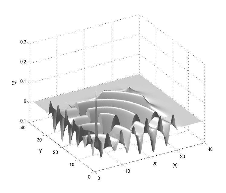
Figure 5: The real part of the 2D wave function of the Three-particle s-wave scattering problem of (49) in the hybrid approach with 40 oscillator states and the oscillator parameter $b=0.8$. The values of $X$ and $Y$ in the oscillator region are chosen as the corresponding classical turning points to show the similar behavior of the wave function in different representations. Compare with Fig. (3). Note the jump in the wave function near the J-matrix and finite difference boundary. This jump clearly indicates the different regions in the representation.

II.3.2 Extracting Scattering information from a wave function in a hybrid representation

As already mentioned at the beginning of this section, the extraction of observables is not always straightforward in the JM method. This mainly comes from the fact that in the original formulations one has to solve the scattering problem and define the scattering parameters simultaneously.

In the hybrid JM-ECS approach in one dimension, once a solution is obtained, we still need to extract the observables. Since the wave function is represented in the asymptotic region with a finite-difference representation, we can use a standard Wronskian technique to extract the scattering amplitude (see section II.1.5).

Obtaining the scattering information from the solution in two dimensions requires the surface integral of section II.1.5. This approach still needs to be elaborated in the hybrid representation. We consider for this discussion a contour $S$ of the surface integral (14) that is piecewise parallel to one of the axes. This is illustrated in Fig. 6. We first integrate $\rho_{2}$ from 0 to a value $R_{k}\in[a,L]$ while fixing $\rho_{1}=R_{k}$. The point $R_{k}$ is located on the finite difference grid in the region where the equation is homogeneous. Typically $R_{k}$ is chosen a few grid points before the end of the real part of the grid. This procedure leads to a line integral parallel to the $\rho_{2}$ axis. We denote it as $I_{2}$.

The second part of the surface integral integrates $\rho_{1}$ from $R_{k}$ to 0 while keeping $\rho_{2}$ equal to $R_{k}$. This is a line integral parallel to the $\rho_{1}$ axis and is denoted as $I_{1}$.

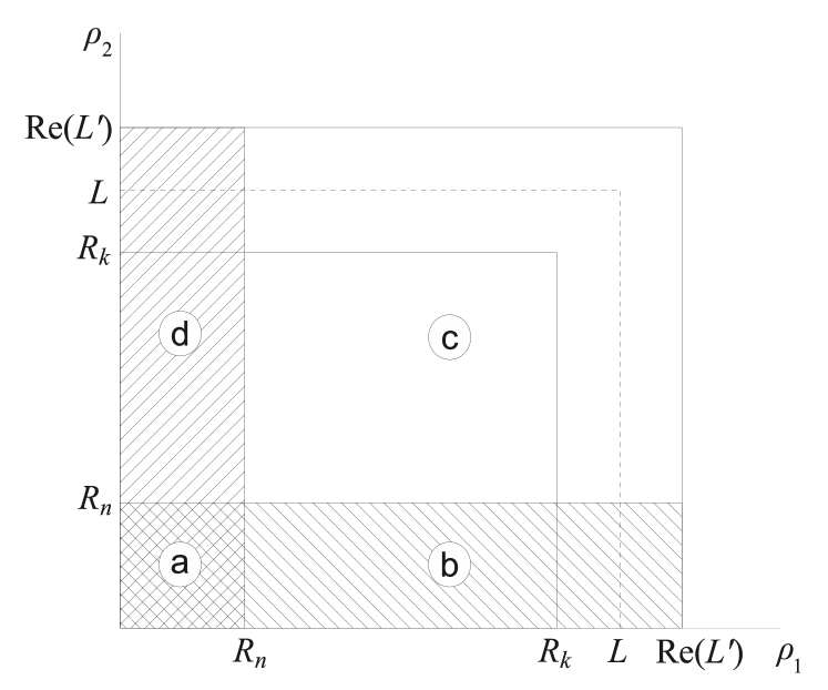
Figure 6: There are four region in the hybrid representation. In region a) $\rho_{1},\rho_{2}<R_{n}$ and the wave function is a sum over product of two oscillator functions. In b) and d) one one coordinate, respectively $\rho_{1}<R_{n}$ and $\rho_{2}<R_{n}$, is represented in the oscillator state. In region c) we use finite difference for both coordinates. The amplitude is calculated with the help of a surface integral along the path that is indicated by the solid line a distance $R_{k}$ away from the axes. Note that between $L$ and Re$(L^{\prime})$ the grid is complex valued because of ECS.

The amplitude, (14), now consists of two parts

$$f_{l_{1},l_{2}}(k_{1},k_{2})=I_{1}+I_{2},$$ (36)

where

$$\begin{split}I_{1}=\frac{1}{2}\int_{0}^{R_{k}}&\left(\tau_{k_{1},l_{1}}(\rho_{1})\tau_{k_{2},l_{2}}(R_{k})\frac{\partial\psi_{sc}(\rho_{1},R_{k})}{\partial\rho_{2}}\right.\\ &\left.-\psi_{sc}(\rho_{1},R_{k})\tau_{k_{1},l_{1}}(\rho_{1})\frac{\partial\tau_{k_{2},l_{2}}(R_{k})}{\partial\rho_{2}}\right)d\rho_{1}\end{split}$$ (37)

and

$$\begin{split}I_{2}=\frac{1}{2}\int_{0}^{R_{k}}&\left(\tau_{k_{1},l_{1}}(R_{k})\tau_{k_{2},l_{2}}(\rho_{2})\frac{\partial\psi_{sc}(R_{k},\rho_{2})}{\partial\rho_{1}}\right.\\ &\left.-\psi_{sc}(R_{k},\rho_{2})\tau_{k_{2},l_{2}}(\rho_{2})\frac{\partial\tau_{k_{1},l_{1}}(R_{k})}{\partial\rho_{1}}\right)d\rho_{2}.\end{split}$$ (38)

This is in fact a surface integral of an in-product of two vector-valued functions. We can reverse the bounds on $I_{1}$ without switching the sign of the argument, since the surface vector also changes direction.

It is important to note that $I_{1}$ probes the 2D wave function $\psi_{sc}(\rho_{1},\rho_{2})$ where it is either represented as a sum over oscillator states in the first coordinate and a finite difference in the second or as a finite difference in both coordinates. The integral never probes the region where both coordinates are represented in the oscillator representation (see region (a) in Fig. 6).

To arrive at a practical expression for the amplitude, we split $I_{1}$ into $\int_{0}^{R_{n}}(\ldots)+\int_{R_{n}}^{R_{k}}(\ldots)$ into an integration from 0 to $R_{n}$, the part covered by the oscillator representation, and an integration from $R_{n}$ to $R_{k}$, covering the grid.

In order to calculate the integrals we require the solutions $\tau_{k_{1},l_{1}}(\rho)$ and $\tau_{k_{2},l_{2}}(\rho)$ of equation (15). We solve these equations also in the hybrid representation. The solutions are vectors $t(k_{1})$ and $t(k_{2})\in\mathbb{C}^{(n+m)}$ representing the numerical solution of $\tau_{k_{1},l_{1}}(\rho)$ and $\tau_{k_{2},l_{2}}(\rho)$, respectively, with $k_{1}^{2}+k_{2}^{2}=E$. For $\rho_{1}\in[0,R_{n}]$ the solution is a finite sum

$$\tau_{k_{1},l_{1}}(\rho_{1})=\sum_{i}^{n-1}t(k_{1})_{i}\phi_{i}(\rho_{1})$$

and, similarly, the 2D wave function in region (b) of Fig. (6) equals $\psi_{sc}(\rho_{1},R_{k})=\sum_{i=0}^{n-1}\mathsf{\Psi}_{ik}\phi_{i}(\rho_{1})$.

The calculation of the amplitude requires the first order derivatives $\partial\tau_{k_{1},l_{1}}(R_{k})/\partial\rho_{1}$ and $\partial\psi_{sc}(\rho_{1},R_{k})/\partial\rho_{2}$. These will be approximated by central differences from $t(k_{1})$ and $\mathsf{\Psi}$. We define

$$t_{k}^{\prime}(k_{1})=\frac{t(k_{1})_{k+1}-t(k_{1})_{k-1}}{2h},$$ (39)

and similarly for $t^{\prime}(k_{2})_{k}$. We also define

$$\mathsf{\Psi}^{\prime,1}_{ik}=\frac{\mathsf{\Psi}_{i+1\,k}-\mathsf{\Psi}_{i-1\,k}}{2h}$$ (40)

and

$$\mathsf{\Psi}^{\prime,2}_{ik}=\frac{\mathsf{\Psi}_{i\,k+1}-\mathsf{\Psi}_{i\,k-1}}{2h}.$$ (41)

So the first term in the integral of $I_{1}$ becomes

$$\begin{split}\int_{0}^{R_{n}}&\left(-\tau_{k_{1},l_{1}}(\rho_{1})\tau_{k_{2},l_{2}}(R_{k})\frac{\partial\psi_{sc}(\rho_{1},R_{k})}{\partial\rho_{2}}\right.\\ &\left.+\psi_{sc}(\rho_{1},R_{k})\tau_{k_{1},l_{1}}(\rho_{1})\frac{\partial\tau_{k_{2},l_{2}}(R_{k})}{\partial\rho_{2}}\right)d\rho_{1}\\ =\int_{0}^{R_{n}}&\left[-\left(\sum_{i=0}^{n-1}t_{i}(k_{1})\phi_{i}(\rho_{1})\right)t_{k}(k_{2})\left(\sum_{j=0}^{n-1}\mathsf{\Psi}^{\prime,2}_{jk}\phi_{j}(\rho_{1})\right)\right.\\ &\!\!\!\!\!\!\!\left.+\left(\sum_{j=0}^{n-1}\mathsf{\Psi}_{jk}\phi_{j}(\rho_{1})\right)\left(\sum_{i=0}^{n-1}t_{i}(k_{1})\phi_{i}(\rho_{1})\right)t_{k}^{\prime}(k_{2})\right]d\rho_{1},\end{split}$$ (42)

where we have used that $\tau_{k_{2},l_{2}}(R_{k})=t_{k}(k_{2})$ since the vector $t(k)$ represents the solution in the hybrid representation. In the next step we reorder the sum and the integral and find

$$\begin{split}=-t_{k}(k_{2})&\sum_{i=0}^{n-1}\sum_{j=0}^{n-1}t_{i}(k_{1})\mathsf{\Psi}^{\prime,2}_{jk}\int_{0}^{R_{n}}\phi_{i}(\rho_{1})\phi_{j}(\rho_{1})d\rho_{1}\\ &+t_{k}^{\prime}(k_{2})\sum_{j=0}^{n-1}\sum_{i=0}^{n-1}t_{i}(k_{1})\mathsf{\Psi}_{jk}\int_{0}^{R_{n}}\phi_{j}(\rho_{1})\phi_{i}(\rho_{1})d\rho_{1}\\ \approx-t_{k}(k_{2})&\sum_{i=0}^{n-1}t_{i}(k_{1})\mathsf{\Psi}^{\prime,2}_{ik}+t^{\prime}_{k}(k_{2})\sum_{i=0}^{n-1}t_{i}(k_{1})\mathsf{\Psi}_{ik}\\ &+\mathcal{O}(\max_{i,j<n}|\int_{R_{n}}^{\infty}\phi_{i}\phi_{j}|).\end{split}$$ (43)

We have used that $\int_{0}^{R_{n}}\phi_{i}\phi_{j}=\delta_{ij}-\int_{R_{n}}^{\infty}\phi_{i}\phi_{j}$.

The second term in the integral $I_{1}$ covers the grid and it is approximated using Simpson’s rule

$$\begin{split}&\int_{R_{n}}^{R_{k}}\left(-\tau_{k_{1},l_{1}}(\rho_{1})\tau_{k_{2},l_{2}}(R_{k})\frac{\partial}{\partial\rho_{2}}\psi_{sc}(\rho_{1},R_{k})\right.\\ &\left.+\psi_{sc}(\rho_{1},R_{k})\tau_{k_{1},l_{1}}(\rho_{1})\frac{\partial}{\partial\rho_{2}}\tau_{k_{2},l_{2}}(R_{k})\right)d\rho_{1}\\ &=-t_{k}(k_{2})\sum_{i=n}^{k}t_{i}(k_{1})\mathsf{\Psi}^{\prime,2}_{ik}w_{i}+t^{\prime}_{k}(k_{2})\sum_{i=n}^{k}\mathsf{\Psi}_{ik}t_{i}(k_{1})w_{i},\end{split}$$ (44)

where $w_{i}$ is the weight of integration. The weight has a value $w_{i}=h$, for all $i$ except at $i=n$ and $i=k$, the end points of integration, where it equals $w_{i}=h/2$. Combining both parts $I_{1}$ and $I_{2}$ one obtains

$$\begin{split}&2f_{l_{1},l_{2}}(k_{1},k_{2})=\\ &t_{k}(k_{1})\sum_{i=0}^{k}t_{i}(k_{2})\mathsf{\Psi}^{\prime,1}_{ki}w_{i}-t^{\prime}_{k}(k_{1})\sum_{i=0}^{k}\mathsf{\Psi}_{ki}t_{i}(k_{2})w_{i}\\ &-t_{k}(k_{2})\sum_{i=0}^{k}t_{i}(k_{1})\mathsf{\Psi}^{\prime,2}_{ik}w_{i}+t^{\prime}_{k}(k_{2})\sum_{i=0}^{k}\mathsf{\Psi}_{ik}t_{i}(k_{1})w_{i},\end{split}$$ (45)

where

$$w_{i}=\begin{cases}1\quad&\text{if}\quad i<n,\\ h/2\quad&\text{if}\quad i=n,\\ h\quad&\text{if}\quad n<i<k,\\ h/2\quad&\text{if}\quad i=k.\end{cases}$$ (46)

The factor 2 in (LABEL:eq:finalamp) comes from the surface integral (14).

III Numerical results

To illustrate and benchmark the proposed hybrid JM-ECS method, we consider two model problems that are derived from a two-body and a three-body problem. When these systems are expressed in spherical coordinates around the center of mass and expanded in spherical harmonics one typically ends up with a large system of coupled radial equations, known as the partial wave equations. These partial waves can either be coupled 1D or coupled 2D problems. We choose to benchmark our methods to model problems formulated as an uncoupled partial wave problem.

The two-body problem reduces to a one-dimensional radial problem with the form given by (7).

Similarly a two-dimensional radial problem is derived from a three-body problem and is, expressed as:

$$\left\{\begin{split}&\left(T_{1}+V_{1}(\rho_{1})+\frac{l_{1}(l_{1}+1)}{2\rho_{1}^{2}}+T_{2}+V_{2}(\rho_{2})+\frac{l_{2}(l_{2}+1)}{2\rho^{2}_{2}}\right.\\ &\hskip 19.91684pt\left.+V_{12}(\rho_{1},\rho_{2})-\frac{k^{2}}{2}\right)\psi_{sc}(\rho_{1},\rho_{2})\\ &\hskip 5.69046pt=-\frac{1}{\sqrt{k_{0}}}\left(\left[V_{2}(\rho_{2})+V_{12}(\rho_{1},\rho_{2})\right]\varphi_{l_{1},0}(\rho_{1})\hat{j}_{l_{2}}(k_{0}\rho_{2})\right.\\ &\hskip 42.67912pt+\left.\left[V_{1}(\rho_{1})+V_{12}(\rho_{1},\rho_{2})\right]\varphi_{l_{2},0}(\rho_{2})\hat{j}_{l_{1}}(k_{0}\rho_{1})\right),\\ &\psi_{sc}(0,\rho_{2})=0\,\,\forall\rho_{1}>0\quad\text{and}\quad\psi_{sc}(\rho_{1},0)=0\,\,\forall\rho_{2}\\ &\text{with outgoing wave boundary conditions for}\\ &\rho_{1}\rightarrow\infty\quad\text{or}\quad\rho_{2}\rightarrow\infty,\end{split}\right.$$ (47)

where $\rho_{1}$ and $\rho_{2}$ are two radial coordinates representing the distances of the first and second particle to the center of the coordinate system. The two body potential is $V_{12}(\rho_{1},\rho_{2})$. The angular momenta $l_{1}$ and $l_{2}$ are non-negative integers.

The total wave function is the sum of an incoming wave and a scattered wave. If we model an impact ionization problem, for example, the incoming wave will be a product of the target in the ground state, $\varphi_{l_{1},0}$ and the incoming wave, $j_{l_{1}}(k_{0}\rho_{2})$, of the second particle. Taking into account symmetrization this is

$$\frac{1}{\sqrt{k_{0}}}\left(\varphi_{l_{1},0}(\rho_{1})\hat{j}_{l_{2}}(k_{0}\rho_{2})+\varphi_{l_{2},0}(\rho_{2})\hat{j}_{l_{1}}(k_{0}\rho_{1})\right),$$

where $\varphi_{l_{1},0}(\rho_{1})$ is an eigenstate of the operator $(T_{1}+V_{1}+l_{1}(l_{1}+1)/2\rho_{1}^{2})$ with energy $E_{0}$. The incoming wave $\hat{j}_{l_{1}}(k_{0}\rho_{1})$ has momentum $k_{0}$ such that $k_{0}^{2}/2+E_{0}=k^{2}/2$.

Note that the method we propose is not only applicable to impact problems but also to other breakup situations. Then the right hand side in (47) can be replaced by any other driving term. In photo-ionization, for example, the right hand side is the dipole operator $\vec{\mu}$ applied to the ground state of the two particle system $\varphi(\rho_{1},\rho_{2})$.

III.1 One dimensional phase shift

To validate the proposed hybrid JM-ECS technique we first solve the one-dimensional scattering problem with an attractive Gaussian potential:

$$\left(-\frac{1}{2}\frac{d^{2}}{dx^{2}}+\frac{l(l+1)}{2x^{2}}-V_{0}\mathrm{e}^{x^{2}/r_{0}^{2}}-\frac{k^{2}}{2}\right)\psi(x)=0,$$ (48)

where the parameters of the potential were chosen as $V_{0}=0.2$ and $r_{0}=2$. We determine the elastic scattering phase shift as a function of the momentum of the incoming particle. To estimate the accuracy of the hybrid results we compare the phase shift to the one obtained with the Variable Phase Approach (VPA) Calogero (1967), which yields the exact result with very high accuracy for this simple problem. In Fig. 7 we display the results for oscillator length $b=0.3$ and increasing matching point $N$; this corresponds to an increasing size of the interaction region, and thus an increasing size of the truncated oscillator basis. It is clear from this figure that the results strongly depend on the choice of the matching point for a required accuracy. In Fig. 8 we display the results for different values of the angular momentum $l$, all seen to be of qualitatively comparable accuracy.

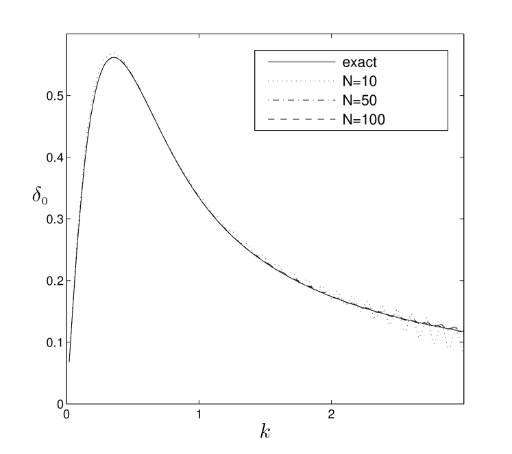
Figure 7: $s$-wave phase shift for a Gaussian potential ($V_{0}=0.2$, $r_{0}=2$) as a function of wave number $k$ for the problem of (48). Shown are the hybrid JM-ECS results for different matching points $N$, and the VPA (exact) result. The oscillator length is $b=0.3$.

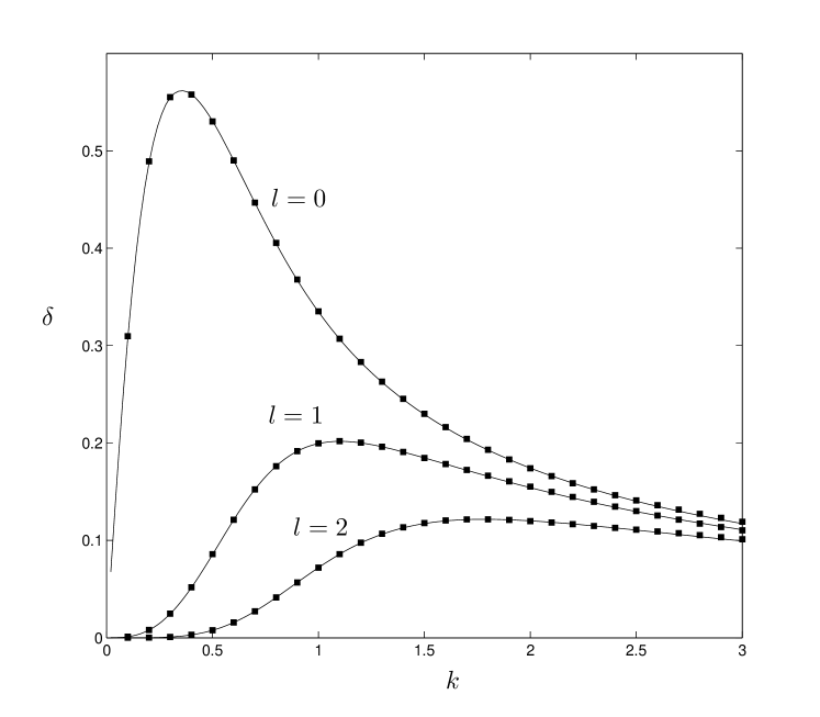
Figure 8: Phase shifts for a Gaussian potential ($V_{0}=0.2$, $r_{0}=2$) of equation (48) and different angular momenta obtained with JM-ECS (squares), compared to VPA results (solid lines). For all results $b=0.3$ and $N=50$.

To quantify the accuracy we display an error plot in Fig. 9 where one notices an increasing accuracy with increasing size of the oscillator basis in the interaction region. The error is seen to decrease in terms of $N$ in both the small- and large-energy region. For large energies the error is mainly caused by the finite-differences approximation to the second derivative. At small energies the error mainly comes from an inaccurate approximate relation (27) which improves as the size of the oscillator basis increases.

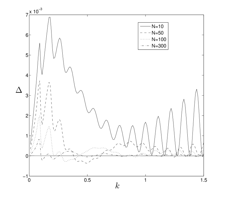
Figure 9: The absolute error in phase shift for different sizes of the oscillator basis (b=0.3, l=0) for model problem of fig. 7 and 7

In table 1 we display the error value for different sizes $N$ of the oscillator basis and for different partial waves. For each partial wave we consider the $k$-value where the error is maximal

$N$	$|\Delta|$ ($\times 10^{-3}$)
	$l=0$	$l=1$	$l=2$
	($k=0.17$)	($k=0.62$)	($k=1.0$)
10	6.9	4.6	3.6
20	7.5	1.7	1.2
50	3.7	0.045	0.039
100	1.4	0.02	0.076
200	0.41	0.18	0.0079
300	0.10	0.12	0.0026

Table 1: Absolute error $\Delta$ in the phase shift for different sizes of the oscillator basis ($b=0.3$).

We observe that the error of the hybrid method has rather intricate and oscillatory behavior in terms of the size, but in general decreases with increasing oscillator basis. Full convergence is however not yet obtained. In any case it is seen that the approach provides relatively stable and accurate results for different values of the angular momenta, energy ranges, and sizes of the oscillator basis.

III.2 $s$-wave benchmark with product two-body potentials

As described above, the hybrid model introduced in this paper is easily extended to systems with more degrees of freedom, in contrast to the original JM method. We demonstrate this on a model breakup problem with a short-range potential taken from Rescigno et al. (1999):

$$\left(-\frac{1}{2}\frac{\partial^{2}}{\partial x^{2}}-\frac{1}{2}\frac{\partial^{2}}{\partial y^{2}}-V_{0}\mathrm{e}^{-x}-V_{0}\mathrm{e}^{-y}\right.\\ \left.+W_{0}\mathrm{e}^{-x-y}-E\right)\Psi=0$$ (49)

with $V_{0}=3$ and $W_{0}=10$. These interaction parameters yield one bound state for the attractive “one-particle” potential $V_{0}$ with an energy $E_{0}=-0.411$. We choose the energy of the incident particle to be $E_{inc}=0.882$ (similarly to Rescigno et al. (1999)) what leads to a total energy of the system $E=0.471$.

Fig. 10 pictures the single differential cross section (SDCS) for the breakup after impact. The escaping particles have an energy of $0.471$ to share between them. Since the two particles are indistinguishable the cross section is symmetric around $0.471/2$. In the figure we also compare with the results of the finite difference calculations. We see a slight difference for equal energy sharing. To highlight the difference we have scaled the vertical axis.

The error between the finite difference calculations and the hybrid method is given in table 2 where we look at the error for a particular energy sharing. As the number of oscillator states increases the results converge.

In Table 2 we display the difference between the results of the hybrid method and those of a full finite-difference calculation in terms of the the size of the oscillator basis $N$.

Figure 10: SCDS results of $s$-wave scattering for model problem (49), for a total energy of 0.471 (solid line — finite differences, dashed line — JM-ECS). The parameters of the calculation are $N$=80 and $b$=0.3. The vertical axis has been rescaled to emphasize the difference.

$N$	$|\Delta|$
10	0.0937
20	0.0836
40	0.0678
60	0.0592
80	0.0184

Table 2: Absolute error $\Delta$ of the hybrid method w.r.t. a full finite-difference approach for the SDCS results of problem (49). The total energy is 0.471, and there is equal energy sharing between the particles.

III.3 More realistic $s$-wave benchmark with Gaussian potential

All potentials in (49) are exponentially decaying in both coordinates, and such a model is not very realistic. In real problems the inter-particle potential depending on the distance between particles should decay significantly slower. We consider a more realistic three-dimensional problem, but similar to the one described above. This could correspond to a scattering problem with two equal, light, particles and a third heavy one:

$$\left(-\frac{1}{2}\Delta_{r_{1}}-\frac{1}{2}\Delta_{r_{2}}-V_{0}\mathrm{e}^{-|\mathbf{r}_{1}|}-V_{0}\mathrm{e}^{-|\mathbf{r}_{2}|}\right.\\ \left.+W_{0}\mathrm{e}^{-|\mathbf{r}_{1}-\mathbf{r}_{2}|^{2}}-E\right)\Psi=0$$ (50)

with $\mathbf{r}_{1}$ and $\mathbf{r}_{2}$ the coordinates of the two (light) particles with respect to the third one. Here we consider a Gaussian form of the potential for the interaction between the light particles to simplify the subsequent calculations, and to obtain a faster-decaying $s$-wave potential. The $s$-wave projection of this equation yields

$$\left(-\frac{1}{2}\frac{\partial^{2}}{\partial x^{2}}-\frac{1}{2}\frac{\partial^{2}}{\partial y^{2}}-V_{0}\mathrm{e}^{-x}-V_{0}\mathrm{e}^{-y}\right.\\ \left.+W_{0}\frac{\left(\mathrm{e}^{-(x-y)^{2}}-\mathrm{e}^{-(x+y)^{2}}\right)}{2xy}-E\right)\Psi=0$$ (51)

In Fig. 11 we show the SCDS for this problem, and compare with the results from a full finite difference calculation. In these calculations we had to increase the size of the finite-difference grid to cover the interaction region, which leads to an increase increasing of the oscillator parameter (see 29). We considered $b=1.3$ in this calculation.

Overall the results are comparable. The small oscillations in the finite difference results come from small numerical reflections at the point of complex scaling. These can be eliminated by using a smooth complex scaling or a PML Berenger (1994) as an absorbing boundary. In a similar way, the hybrid method result also shows comparable oscillations.

Table 3 shows the errors in the SDCS as a function of the oscillator basis size. Comparing the error values with the value of SDCS we can see that the relative error is considerably bigger than in previous problem. Apart of the increased complexity of the problem, the reason for this is that the asymptotic relation (27) becomes less accurate with an increase of the oscillator parameter $b$.

Figure 11: SCDS results of s-wave scattering for model problem (51) with a Gaussian two body potential (solid line — finite differences, dashed line — JM-ECS). The parameters of the calculation are $N$=70 and $b$=1.3.

$N$	$|\Delta|$
10	0.3730
20	0.0221
30	0.0776
50	0.0685
70	0.0153

Table 3: Absolute error $\Delta$ of the hybrid method w.r.t. a full finite-difference approach for the SDCS results of problem (51). The total energy is 0.471, and there is equal energy sharing between the particles.

IV Application to nuclear $p$-shell scattering

In this section we go beyond model problems and apply our method in the more realistic context of $\alpha$-scattering in $p$-shell nuclei Sytcheva et al. (2006), in particular ${}^{8}Be$ Sytcheva et al. (2006).

This is a commonly used benchmark problem in nuclear cluster physics. We will perform an $\alpha-\alpha$ scattering calculation including fully microscopic states for the interaction region, and using a semi-realistic nucleon-nucleon interaction. We compare the results with those obtained in the JM approach.

In the asymptotic region the system decays into two point particles, each corresponding to an $\alpha$-particle. At closer distances, however, the internal structure of the clusters becomes of importance because of the microscopic interactions and the Pauli exchanges between nucleons.

The cluster basis states have the form

$$\Psi_{nL}=\widehat{\mathcal{A}}\left\{\Phi_{1}\left(\alpha\right)\Phi_{2}\left(\alpha\right)\phi_{nL}\left(\mathbf{r}\right)\right\},$$ (52)

where $\widehat{\mathcal{A}}$ is the antisymmetrization operator, and $\Phi_{1,2}\left(\alpha\right)$ is a translation invariant shell-model state built up of $s$-orbitals for the $\alpha$-particles. The state $\phi_{nL}\left(\mathbf{r}\right)$ is a three-dimensional harmonic oscillator state for the relative motion of the $\alpha$-clusters

$$\phi_{nL}\left(\mathbf{r}\right) = \phi_{n+n_{0},LM}\left(\mathbf{r}\right)$$

$$= \mathcal{N}_{n+n_{0},L}~{}\rho^{L}e^{-\rho^{2}/2}L_{n+n_{0}}^{L+1/2}\left(\rho^{2}\right)Y_{LM}\left(\widehat{\mathbf{r}}\right)$$

$$\rho = \frac{\left|\mathbf{r}\right|}{b},\quad\mathcal{N}_{nL}=\sqrt{\frac{2\Gamma\left(n+1\right)}{\Gamma\left(n+L+3/2\right)}}$$

We use $n_{0}$ to denote the minimal value of the shell number allowed by the Pauli exclusion principle

$$n_{0}=\begin{cases}(N_{min}-L)/2&\text{for }L<N_{min},\\ 0&\text{for }L\geq N_{min},\end{cases}$$ (54)

where $N_{\min}$ is the number of oscillator quanta in that shell.

$$N_{\min}=\begin{cases}A-4,&\text{normal parity states: }\pi=\left(-1\right)^{A}\\ A-3,&\text{abnormal parity states: }\pi=\left(-1\right)^{A+1}\end{cases}$$ (55)

In this form $n=0,1,...$ numerates all the Pauli allowed states for the cluster relative motion. For all further details, we refer to Sytcheva et al. (2006) and Sytcheva et al. (2006).

A common nucleon-nucleon interaction used for this sytem is a Volkov N1 (V1) potential, which can be written in the form

$$V_{ij}={\displaystyle\sum\limits_{k=1}^{2}}V_{k}(1+mP_{ij}^{r})\exp\{-(r_{ij}/a_{k})^{2}\},$$ (56)

where $m$ is the Majorana exchange parameter. The strength parameters $V_{k}$ determine the repulsive short-range core and the long-range attraction. We take the same parameters as in Sytcheva et al. (2006) and Sytcheva et al. (2006), but omit the Coulomb interaction between protons to simplify the effective asymptotic $\alpha-\alpha$ interaction.

The calculations of matrix elements in the internal region is identical as in the JM approach. The difference lies in the asymptotic region, where the explicit asymptotic potential, expanded in the oscillator basis, is now replaced by the finite differences approach, as discussed in section II.3, after proper matching of both regions; the asymptotic $\alpha-\alpha$ interaction reduces to the point-like effective free particle kinetic energy between the two clusters.

In Fig. 12 we show the $J^{\pi}=0^{+},2^{+}$ and $4^{+}$ phase shifts for the ⁸Be system calculated with the hybrid JM-ECS and JM approaches. For the latter we take results as they have been obtained in Sytcheva et al. (2006), where a modified JM approach was considered, providing faster convergence Vanroose et al. (2001); we refer to such calculation as MJM for consistency. The overall results are very close to each other. The only noticeable discrepancies occur at very low energies. The difference between MJM and JM-ECS phase shifts in this region is presented in Fig. 13. The oscillations in this difference correlate with the value of the derivative of the wave function in the matching point between the two representations. The source of the error is a “reflection” from this point, and an improvement of the method to reduce this discrepancy is currently under research.

Figure 12: Scattering phase shifts for the $\alpha-\alpha$ system for different values of total angular momentum calculated with MJM (solid lines) and hybrid JM-ECS method (closed squares). All calculations were made with 80 oscillator states

Figure 13: Difference between MJM and JM-ECS scattering phases for the 2⁺ state of the $\alpha-\alpha$ system.

V Discussion and Conclusion

This article reports on initial efforts to introduce absorbing boundary conditions in quantum scattering problems where the wave function is represented by a finite sum of oscillator states. We have introduced the exterior complex scaling (ECS) boundary conditions by constructing a representation of the wave function that combines the oscillator states with a grid based representation. The oscillator representation covers the inner region of the problem, where the main interaction occurs, while the grid covers the near field. The two regions are numerically matched at an interface using an asymptotic expression for the expansion of oscillator states.

The far field amplitude, which gives the cross section, is extracted from the numerical wave function using a surface integral. Extra care is required in the calculation of this integral in this representation.

We have numerically solved several benchmark problems and compared our results with literature and plain ECS calculations.

Our results agree with existing methods and confirm that the proposed method works. However, the accuracy still needs to be improved. This can be done by including mixed potential matrix elements from different representations, by using a different finite difference grid, or by using a higher order matching condition at the interface between the oscillator representation and the finite difference representation. Also a proper treatment of the Coulomb interaction and other effective interactions with long-range behavior must be considered in the future development of the method.

The building blocks presented in this papers are the starting point for a fully coupled calculations similar to Vanroose et al. (2005). In such a calculation the wave function is a sum over $l_{1}$, $m_{1}$ and $l_{2}$, $m_{2}$ of 2D functions $\psi_{l_{1}m_{1},l_{2}m_{2}}$ combined with $Y_{l_{1}m_{1}}(\Omega_{1})Y_{l_{2}m_{2}}(\Omega_{2})$. The linear system is then a coupled system where each diagonal block is a system like eq. (47). From such a representation of the wave function we can extract not only the single differential cross section, but also the triple differential cross section, which gives the amplitude for certain breakup directions. In a similar way, the method can be applied to different multi-channel calculations of three-cluster systems and different reaction processes with light nuclei. In all such problems asymptotic description can be greatly simplified if we use absorbing boundary conditions.

We conclude that it is possible to introduce a boundary layer that absorbs all outgoing waves within a spectral basis such as the oscillator representation.