Hidden possibilities in controlling optical soliton in fiber guided doped resonant medium

Fiber guided optical signal propagating in a Erbium doped nonlinear resonant medium is known to produce cleaner solitonic pulse, described by the self induced transparency (SIT) coupled to nonlinear Schrödinger equation. We discover two new possibilities hidden in its integrable structure, for amplification and control of the optical pulse. Using the variable soliton width permitted by the integrability of this model, the broadening pulse can be regulated by adjusting the initial population inversion of the dopant atoms. The effect can be enhanced by another innovative application of its constrained integrable hierarchy, proposing a system of multiple SIT media. These theoretical predictions are workable analytically in details, correcting a well known result.

I. INTRODUCTION

Optical communication through fiber has achieved phenomenal development over the last two decades [1]. Dissipation and dispersion in the media, which are the main hindrances in signal transmission, are usually attempted to be solved by the dispersion management techniques and devices [1, 2]. On the other hand, in soliton based optical communication, mediated by the nonlinear Schrödinger (NLS) equation proposed much earlier [3], the group velocity dispersion can be countered by the self phase modulation in the nonlinear fiber medium [4]. However, the experiments revealed insufficiency of the model for its efficient practical application [5]. Another proposal with improved solitonic transmission was due to the self-induced transparency (SIT), produced by the coherent response of the medium to an ultra short optical pulse [6, 7]. Finally, the benefits of both the NLS and the SIT systems, were combined in a coupled NLS-SIT model [8], by transmitting the optical soliton through an Erbium doped nonlinear resonant medium [9, 10].

However the solitonic communication, in spite of its favorable features and theoretical advantages due to its underlying integrability, did not receive the needed response. Our aim here therefore, is to revisit the NLS-SIT model for exploring new possibilities hidden in its integrable structures and use them for the control and amplification of the solitonic pulse. Though the soliton usually moves with a constant velocity or speed, the integrable property of this coupled NLS-SIT system, as we find here, allows the soliton speed to be a tunable function. And since the soliton width in this case is related to its speed, which in turn is linked here to the initial population inversion, the pulse width can be regulated by manipulating the population inversion profile of the dopant atoms. This controlling effect can be further enhanced by exploring another specialty of this integrable system, namely its constrained integrable hierarchy, through a novel use of coupled multiple SIT media, in place of the conventional single doped medium. The details can be worked out exactly due to the integrability of the model, detecting the limitation of a well known result on NLS-SIT soliton [9, 10].

Propagation of a stable optical pulse through a fiber medium, serving as a dispersive and nonlinear wave guide with Kerr nonlinearity [3], can be described by the optical electric field $E(z,t)$ satisfying the well known NLS equation

$$\ iE_{z}-E_{tt}-2|E|^{2}E=0,\$$ (1)

with space and time variables being interchanged as customary in nonlinear optics [4]. On the other hand, ultra short optical pulse producing SIT in the medium can be described by the Maxwell-Bloch equation [6, 7]

$$iE_{z}=2p,\ \ ip_{t}=2NE,\ iN_{t}=-(Ep^{*}-E^{*}p),$$ (2)

with the induced polarization $p$ and the population inversion $N$ of the medium, contributed by the Bloch equation. Fascinatingly, it is possible to combine these two effects by transmitting the stable nonlinear pulse produced in the fiber wave guide through a doped medium with coherent response, governed by a coupled NLS-SIT system given by a deformed NLS equation

$$iE_{z}-E_{tt}-2|E|^{2}E=2p_{1},\$$ (3)

together with the SIT equations

$$ip_{1t}=2(N_{1}E-w_{0}p_{1}),\ iN_{1t}=-(Ep_{1}^{*}-E^{*}p_{1}),$$ (4)

representing a nonholonomic constraint [12]. In (4) , $\ p_{1}=\nu\tilde{\nu}^{*}$ is the induced polarization and $N_{1}=|\tilde{\nu}|^{2}-|\nu|^{2},\ -1\leq N_{1}\leq 1,\$ is the population inversion of the two level dopant atoms with normalized wave functions $\nu,\ \tilde{\nu}$ for the ground and the excited states, respectively and $w_{0}$ is the natural frequency of these resonant ions. Assuming a homogeneous broadening of the frequency spread with a sharp resonance at $\Delta w=w-w_{0}$, we have taken the symmetric distribution $g(\Delta w)=\delta(\Delta w)$ and replaced the average value $<p_{1}>=\int dwg(\Delta w)p_{1}(z,t,w)$ appearing in (3) by $p_{1}=p_{1}(z,t,w_{0})$ and normalized the coupling constants to ensure the integrability of the model.

II. INTEGRABILITY AND SOLITON SOLUTION

Recall that, an integrable nonlinear equation may be associated with a linear system $\Phi_{t}=U\Phi,\ \Phi_{z}=V\Phi,$ defined through a Lax pair $U(\lambda),V(\lambda)$, which are matrices with their elements depending on the basic fields and a parameter $\lambda$, known as the spectral parameter. Through compatibility of the linear Lax equations, inducing flatness condition: $U_{z}-V_{t}+[U,V]=0,$ the Lax pair yield the given nonlinear equation and at the same time can be used to extract its exact solutions through the inverse scattering method (ISM) [11]. We remind again that, the space $z$ and time $t$ are interchanged here in the context of nonlinear optics. It is noteworthy that, while the set of coupled NLS-SIT equations (3-4) generalize both the NLS (1) and the SIT (2) equations, the associated Lax pair $U_{nls:sit},V_{nls:sit}$ contain these subsystems as the constituent parts:

$$U_{nls:sit}(\lambda)=U_{nls}(\lambda)=U_{sit}(\lambda),\ \ \ V_{nls:sit}(\lambda)=V_{nls}(\lambda)+V_{sit}(\lambda)$$ (5)

where $U_{nls},V_{nls}$ and $U_{sit},V_{sit}$ are the Lax pairs related to the NLS and the SIT equations, respectively. The NLS Lax pair is well known as [11]

$$U_{nls}(\lambda) = i(\sigma^{3}\lambda+U^{(0)}),\ U^{(0)}=E\sigma^{+}+E^{*}\sigma^{-}$$ (6)

$$V_{nls}(\lambda) = V^{(0)}+V^{(1)}\lambda+V^{(2)}\lambda^{2},\$$

$$V^{(0)} = (U_{x}^{(0)}-i(U^{(0)})^{2})\sigma^{3},\ V^{(1)}=2iU^{(0)},\ V^{(2)}=2i\sigma^{3},$$ (7)

where $\sigma^{3},\ \sigma^{\pm}=\frac{1}{2}(\sigma^{1}\pm i\sigma^{2})$ are the $2\times 2$ Pauli matrices. The SIT Lax pair can be given by the same time-Lax operator as that of the NLS: $U_{sit}(\lambda)=U_{nls}(\lambda),$ while the space-Lax operator

$$V_{sit}(\lambda)=i(\lambda-w_{0})^{-1}G_{1},\ G_{1}=N_{1}\sigma^{3}+p_{1}\sigma^{+}+p^{*}_{1}\sigma^{-},$$ (8)

can be linked to the nonholonomic deformation [12]. We check easily that, the flatness condition of (6,7) yields the NLS equation (1), while (6,8) the SIT equation (2) and similarly, the Lax pair (5) would yield the coupled NLS-SIT equations (3,4)

The time-Lax operator $U(\lambda)$ plays the central role in the ISM for finding the exact solutions of the nonlinear equation [11] and therefore, since $U(\lambda)$ is the same for NLS (1), SIT (2) and NLS-SIT (3,4) equations as seen from (5), the form of soliton solutions and the ISM procedure are remarkably similar for all the three equations. We therefore present soliton solutions for all of them in an unified way following the ISM [11], which though an involved method, gives the 1-soliton solution in an amazingly simple form:

$$E=c\ \frac{g}{1+|g|^{2}},\ \ g={\rm exp}[2i({\rm u}^{\infty}t+\tilde{\rm v}^{\infty}z+\phi)],$$ (9)

with $c,\phi=$ constants. Note that, the crucial elements ${\rm u}^{\infty},\tilde{\rm v}^{\infty}=\frac{1}{z}\int^{z}dz{\rm v}^{\infty}$ in (9), though linked to the Lax pair of the given system, need information only about their asymptotic properties: ${\rm u}^{\infty}=\sigma^{3}U(\lambda_{1})|_{t=-\infty},\ {\rm v}^{\infty}=\sigma^{3}V(\lambda_{1})|_{t=-\infty},$ at discrete spectral parameter $\lambda_{1}$. Therefore, fixing the initial condition of the basic fields involved in the NLS-SIT equations as

$$E(z,t=-\infty)\to 0,\ p_{1}(z,t=-\infty)\to 0,N_{1}(z,t=-\infty)=N_{0}(z)$$ (10)

with an arbitrary function $N_{0}(z),$ we can easily derive from the Lax pair (5-8):

$$\sigma^{3}{\rm u}_{nls:sit}^{\infty} = U_{nls:sit}(\lambda_{1})|_{t=-\infty}=U_{nls}(\lambda_{1})|_{t=-\infty}=U_{sit}(\lambda_{1})|_{t=-\infty}=2i\sigma^{3}\lambda_{1},$$

$$\sigma^{3}{\rm v}_{nls:sit}^{\infty} = V_{nls:sit}(\lambda)|_{t=-\infty}=(V_{nls}(\lambda)+V_{nls}(\lambda))|_{t=-\infty}=i\sigma^{3}(2\lambda_{1}^{2}+(\lambda_{1}-w_{0})^{-1}N_{0}(z)),$$ (11)

which at the discrete spectral parameter with complex value: $\lambda_{1}=k+i\eta,$ take the explicit form

$${\rm u}_{nls:sit}^{\infty}=i\lambda_{1},\ {\rm v}_{nls:sit}^{\infty}={\rm v}_{nls}^{\infty}+{\rm v}_{sit}^{\infty},\ {\rm v}_{nls}^{\infty}=2i\lambda_{1}^{2},\ {\rm v}_{sit}^{\infty}=i(\lambda_{1}-w_{0})^{-1}N_{0}(z).$$ (12)

Inserting the needed complex valued expressions (12) in (9) and grouping its real (Re) and imaginary (Im) parts we get the 1-soliton solution for the optical field in NLS-SIT equations (3,4) in the familiar $sech$- form

$$E=-2i\eta\ {\rm sech}2\zeta e^{2i\theta},\ \zeta=\eta(t-t_{0}-vz),\ \theta=\omega z+kt+\phi_{0},$$ (13)

where $t_{0}$ and $\phi_{0}$ are constant time and phase shift. Inverse speed $v$ and phase rotation $\omega$ for the NLS-SIT soliton (13) are given by the superposition

$$v=v_{nls}+v_{sit},\ \omega=\omega_{nls}+\omega_{sit},$$ (14)

of the corresponding parameters from the NLS and the SIT subsystems, derived from (12) using $\lambda_{1}=k+i\eta$ as

$$v_{nls}=-\frac{1}{\eta}{Im[{\rm v}_{nls}^{\infty}]}=-4k,\ \omega_{nls}=Re[\tilde{\rm v}_{nls}^{\infty}]=2(k^{2}-\eta^{2}),$$ (15)

$$v_{sit}=-\frac{1}{\eta}Im[\tilde{\rm v}_{sit}^{\infty}]=\frac{1}{\rho}{f(z)},\ \omega_{sit}=Re[\tilde{\rm v}_{sit}^{\infty}]=\frac{\tilde{k}}{\rho}{f(z)},$$ (16)

with $\tilde{k}=k-w_{0},\ \rho={\tilde{k}}^{2}+\eta^{2},$ and $f(z)=\frac{1}{z}\int^{z}N_{0}(z^{\prime})dz^{\prime}$.

It is intriguing to note that, since the z-evolution of the optical field $E$ in the NLS-SIT model follows the superposition rule (14) contributed separately by the NLS and the SIT parts, the term $iE_{z}$ in equation (3), evolving according to solution (13), breaks up into two parts: one follows the NLS contribution with parameters (15) and satisfies the pure NLS part of the equation in the left hand side, while the other part equates to the SIT deformation $2p_{1}$ in the right hand side of (3) involving the related parameters (16). Using this dynamics we derive the soliton solution for the dipole $p_{1}$ from (13), in the form

$$p_{1}=\ \frac{\eta}{\rho}\ N_{0}{\rm sech}2\zeta(i\tilde{k}-\eta{\rm tanh}2\zeta)e^{2i\theta},\\$$

with $\zeta,\theta$ as expressed in (13). Inserting solutions (13, Hidden possibilities in controlling optical soliton in fiber guided doped resonant medium ) for $E$ and $p_{1}$ in (4) and integrating by $t$ we derive further the solution for population inversion

$$N_{1}=N_{0}(1-\frac{\eta^{2}}{\rho}\ {\rm sech}^{2}2\zeta),$$ (17)

again in the solitonic form with arbitrary function $N_{0}(z)=N_{1}(t\to-\infty)$, adjusted by the integration constant. We obtain thus the complete set of exact soliton solutions to the NLS-SIT equations (3-4) as (13) for the optical field $E$, ( Hidden possibilities in controlling optical soliton in fiber guided doped resonant medium ) for the dipole $p_{1}$ and (17) for the population inversion $N_{1}$. A beautiful interaction pattern can be noticed in these solutions, manifested in the superposition relations: $v=v_{nls}+v_{sit},\ \omega=\omega_{nls}+\omega_{sit}$, for the solitonic parametersappearing in (13,14). Intriguingly, in the absence of the SIT system with $p_{1}=N_{1}=0$, when the coupled NLS-SIT equations reduce to the NLS equation (1) for the field $E$, one recovers from (13) the well known NLS soliton by simply putting $v_{sit}=\omega_{sit}=0$ due to the vanishing of (8). Therefore, the NLS soliton takes exactly the same form as (13), though the parameters are reduced to pure NLS case: $v=v_{nls},\ \omega=\omega_{nls}$. Similarly, we can directly get the soliton solution for the pure SIT equations (2) in the same form (13, Hidden possibilities in controlling optical soliton in fiber guided doped resonant medium ,17), but with soliton parameters reducing to $v=v_{sit},\ \omega=\omega_{sit}$, due to switching off the NLS influence: $v_{nls}=\omega_{nls}=0$. Thus our exact NLS-SIT soliton can reproduce the solutions for both the NLS and the SIT equations in a unified way, consistent with the ISM. However this rich interaction picture seems to have been missed in a well known earlier work [9, 10], leading to wrong conclusions in the general case. In particular, the soliton solution for the NLS-SIT equation presented in [9, 10] gives the expression for the pulse delay as $\delta=\frac{n}{c}(1+\gamma)$ ((4.9) in [10]), which is equivalent to the inverse soliton speed for the SIT ((2.22) in [10]), i.e.  $v\equiv\delta=v_{sit}$, in our notation [13]. Similarly, the phase rotation in [9, 10] is given as $\alpha=2\eta^{2}$, meaning $\omega\equiv\alpha=-\omega_{nls}$, (at $k=0$, see (15)) in our notation [13]. Both these results for the coupled NLS-SIT equations appear to be incomplete, when compared with our exact result (14). It is clear that, the solution of [9, 10] can be justified only in a very limited sense, when $v_{nls}=\omega_{sit}=0$ and therefore unlike our soliton solution can not interpolate between the solutions of the NLS and the SIT equations.

This partial result unfortunately led to wrong conclusions, for the NLS-SIT system in general, stating that (sect. IV [10]), the normalized speed (i.e. $\delta^{-1}$) of the NLS-SIT soliton is determined only by the SIT effect and similarly, the z dependence of the phase of the dipole (i.e. $\alpha$) is determined solely by the nonlinear phase change due to the NLS soliton. Our exact solutions for the optical field $E$ (13) and the dipole $p_{1}$ ( Hidden possibilities in controlling optical soliton in fiber guided doped resonant medium ) with correct expressions (14), conclude on the other hand that, only a part (i.e. $v_{sit}$) in the normalized speed $v^{-1}=(v_{nls}+v_{sit})^{-1}$ of the NLS-SIT soliton is determined by the SIT effect, while there is an additional contribution coming from the NLS part $v_{nls}$. Similarly, the z dependence of the phase of the dipole and the input optical field gets contribution from both the NLS and the SIT parts as $\omega=\omega_{nls}+\omega_{sit}$, consistent with the interaction picture in the coupled NLS-SIT system.

III. CONTROLLING OPTICAL SOLITON EXPLOITING INTEGRABLE STRUCTURES

Based on the integrable structures underlying the NLS-SIT system describing the propagation of optical soliton in fiber guided doped medium, we propose two possible ways for controlling the amplitude and width of the optical pulses.
A. Soliton control by regulating initial population inversion
It is commonly believed that, the exact soliton solution of a homogeneous equation always moves with a constant speed, width and frequency, as in the case of the NLS soliton (15) with constant values for $v_{nls},\omega_{nls}$. However, it is crucial to note that, for the NLS-SIT soliton the parameters $(v,\omega)$, as evident from (14,16) can become variable functions, depending on the initial population inversion $N_{0}(z)$ (10). Due to this peculiarity of integrable structure of the NLS-SIT system, hidden in the expressions like (5,8,12,16), the soliton speed: $v^{-1}$ and width: $(\eta v)^{-1}$, as defined from the soliton argument $\zeta$ (13), can be variable and linked to a controllable arbitrary function $N_{0}(z)$.

We show that, this important observation embedded in the integrability of the NLS-SIT system can open up a new avenue for controlling the optical soliton propagating through the doped medium, by regulating its initial population inversion profile $N_{0}(z)$. This fact however remained unexplored in earlier investigations [9, 10, 14, 15], due to the restriction to a fixed initial profile $N_{0}(z)=-1$. Note that, at this particular value giving $f(z)=-1$, our more general result (16) reduces to the simplified expressions obtained earlier:

$$v_{sit}=-\frac{1}{\rho},\ \omega_{sit}=-\frac{\tilde{k}}{\rho},$$ (18)

The choice for the initial population inversion in the NLS-SIT model as an arbitrary function $N_{0}(z)>-1$, that we propose here, gives us the needed freedom for obtaining the excited and the ground state occupancies at the initial moment as $|\tilde{\nu}|^{2}=\frac{1}{2}(1+{N_{0}(z)})$ and $|\nu|^{2}=\frac{1}{2}(1-{N_{0}(z)})$, respectively. Therefore, for $N_{0}>-1$, giving $|\tilde{\nu}|^{2}>0$, we can prepare the dopant atoms initially in an excited state by optical prepumping, resulting to the creation of a laser-active amplifying medium with its intensity determined by $N_{0}$. Note that, only in such a case when more active dopant atoms are in the excited state, the optical soliton can gain net energy [1].

In addition to the soliton pulse amplification, variable initial profile $N_{0}(z)>-1$, permitted by the integrability of the NLS-SIT system, can play a crucial role in controlling the shape and dynamics of the optical soliton. It is possible, as we see below, to address the important problem of pulse broadening by regulating the initial profile of the dopant atoms. For example, a solitonic pulse governed by the NLS equation under small perturbation by a term $-i\frac{\Gamma}{2}E$ with $\ \Gamma<<1$, would suffer broadening by a factor $(4k\eta(z))^{-1}$, which can be worked out through the variational perturbation method as $\eta(z)=\eta\ e^{-\Gamma z}$[4], which is valid however upto the range $\Gamma z\approx 1$ along $z$. Beyond this range with $z>>1$, as shown by some other method, the broadening of the pulse width follows a different rule, by increasing linearly with $z$ at a rate slower than the linear medium [4]. Though an attenuation with intensity loss would also occur simultaneously, the broadening leads to more serious problem of information loss and bandwidth limitation. Therefore we concentrate here only on the broadening problem of the perturbed NLS soliton, due to the increasing solitonic width $\frac{1}{4k\eta}\ e^{\Gamma z}$ along $z$, as shown in Fig 1. As stated above for $z>>1$ it would follow a different rule. We show that, by transmitting this solitonic pulse through a doped resonant medium, described by an interacting NLS-SIT model (3-4), it is possible to control the pulse broadening, by suitably preparing the initial population inversion profile $N_{0}(z)$. Fig 2a shows this controlling effect, where the broadening of the solitonic pulse suffered in Fig 1, is countered by the narrowing of the pulse due to variable width $V(z)=(v_{nls}+N_{0}(z)/(\rho\Gamma))^{-1}$, by taking $N_{0}(z)\sim\eta(z)^{-1}$. Note that the profile $N_{0}(z)$ has to be adjusted differently at different ranges, as mentioned above, to control the broadening in the respective regions for a wide range of $z$. The soliton dynamics would also change to a variable speed $V(z)$, possible due to the energy supplied by optical prepumping.

This potential opportunity for controlling the pulse width, hidden in the integrable property of the NLS-SIT system, as explained above, was missed in earlier investigations [9, 10, 14, 15], since the initial atoms are usually taken in their ground state: $\ |\nu|^{2}=1,\ |\tilde{\nu}|^{2}=0,$ by restricting to $N_{0}(z)=-1$.

Figure 1: Broadening of the perturbed NLS soliton $|E(z,t)|$ along the fiber, moving with a constant speed with parameter choice $k=0.25,\ \eta=0.50,\ \Gamma=0.28$

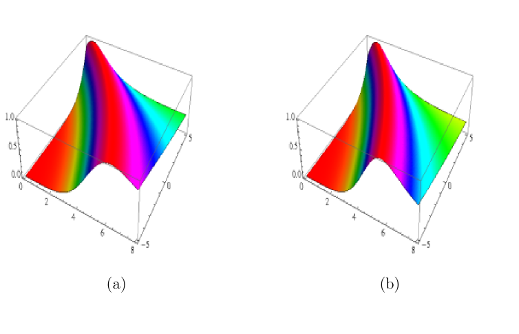
Figure 2: a) Broadening NLS soliton pulse is controlled by a coupled NLS-SIT system with $\ N_{0}(z)=-0.11e^{\Gamma z}$ and $w_{0}=0.3$. Variable speed of the soliton is evident from its bending in the ($z,t$)- plane. b) Additional control is achieved by coupling to a second SIT system with $N^{(2)}_{0}(z)=0.11e^{\Gamma z},\$ showing an efficient restoration of the soliton width.

B. Enhanced soliton control through multiple doping

Another promising opportunity in managing optical soliton in fiber communication, emerging also from the integrability of the NLS-SIT model, is overlooked completely in earlier investigations. This is the proposal of enhancing the effect of amplification and control of the optical soliton by replacing the conventional single SIT system, the only case considered in the literature, by a coupled multiple SIT system, using recursively the constrained integrable hierarchy in the NLS-SIT model (see Fig. 3). The physical meaning of coupling the NLS equation to such multi SIT system can be given through a novel proposal of using coupled multiple doped resonant media, in place of a single doped medium.

For generating the governing hierarchal equations and showing their integrability, we extend Lax operator $V(\lambda)$ (5,8) by adding more deforming terms $V_{sitM}=i\sum_{j}^{M}(\lambda-w_{0})^{-j}G_{j}$, linked to the $M$-th constrained hierarchy [12] in the NLS-SIT system, fixed at level $M$ from the possible infinite sequence : $j=1,2,\ldots$. In analogy with $G_{1}$ (8) we can express the deforming matrices $G_{j}$, through dipole moment $p_{j}$ and population inversion $N_{j}$ of the $j$-th doped resonant medium. For explicit demonstration we restrict to the next higher level $M=2$ in the constrained hierarchy, by considering only an additional SIT system to the original NLS-SIT set. Compatibility of the Lax pair thus defined would generate an extended set of equations given by the same deformed NLS (3) coupled however to a double SIT system

$$ip_{1t} = 2(N_{1}E-w_{0}p_{1}-p_{2}),\ iN_{1t}=-(Ep_{1}^{*}-E^{*}p_{1}),$$

$$ip_{2t} = 2(N_{2}E-w_{0}p_{2}),\ iN_{2t}=-(Ep_{2}^{*}-E^{*}p_{2}),$$ (19)

with induced polarization $p_{2}$ and population inversion $N_{2}$, linked to the additional doped medium described by the second SIT system. We find intriguingly that, the exact soliton solution for the optical pulse $E$ in this extended NLS-SIT model (3,19), can be expressed again in the same form (13), where the soliton parameters are to be modified with contributions from all its interacting parts, i.e. from the NLS as well as from the multiple SIT system as $\ v=v_{nls}+v_{sit1}+v_{sit2},\ \ \omega=\omega_{nls}+\omega_{sit1}+\omega_{sit2}.\$ Parameters $v_{nls},\omega_{nls}$ and $v_{sit1},\omega_{sit1}$ have the same expressions as found already in (15,16), while the additional SIT contribution $v_{sit2},\omega_{sit2}$, can be derived following a similar argument as (16) in the form

$$v_{sit2} = -\frac{1}{\eta}Im[(\lambda_{1}-w_{0})^{-2}]{f_{2}(z)}=2\frac{\tilde{k}}{\rho^{2}}{f_{2}(z)},$$

$$\omega_{sit2} = Re[(\lambda_{1}-w_{0})^{-2}]{f_{2}(z)}=2\frac{\tilde{k}^{2}-\eta^{2}}{\rho^{2}}{f_{2}(z)},$$ (20)

with $f_{2}(z)=\frac{1}{z}\int^{z}N_{0}^{(2)}(z^{\prime})dz^{\prime},$ involving an additional arbitrary function $N_{0}^{(2)}(z)=N_{2}(z,t=-\infty).$ It opens up therefore another novel way, hidden again in the integrable structure of the NLS-SIT system, for an enhanced control of the soliton width and dynamics, by adding a coupled second SIT system, as shown in Fig. 2b.

This process of coupling the NLS equation to the set of multiple SIT equations can be continued within the framework of the integrable system, as mentioned above, creating a form of directional connected network with feedback, as shown in Fig. 3. In particular, as evident from the coupled equations (3,19), the input optical pulse $E$ would influence the dipole field $p_{j}$ and the population inversion $N_{j}$ in all the resonant SIT media with $j=1,2,\ldots,M$, while only $p_{1}$ from the first medium gives feed back to the field $E$. On the other hand, $p_{j+1}$ are coupled sequentially to $p_{j}$, across the media, while $N_{j}$ are mutually coupled only with $p_{j}$ from the same medium, in the multiple SIT system with $j\in[1,M]$. This network, would exhibit more and more manipulative power for control over width and amplification of the optical pulse, enhanced sequentially by choosing a set of initial condition $N_{0}^{(j)}(z)=N_{j}(z,t=-\infty),j=1,2,\ldots M$ and is based on the notion of constrained hierarchy of the integrable NLS-SIT system (see Fig. 3).

Figure 3: Connected network of the NLS and the multiple SIT system with $E$ as the input optical field, $p_{j}$ as the induced polarization and $N_{j}$ as the population inversion of the $j$-th doped resonant medium with $j=1,2,3,\ldots,M$. The arrows show the directions of coupling with equations (3,19) describing this network in the particular case of $M=2$. Sequential enhancement of the control of width and amplification are predicted by this network, which is consistent with the constrained integrable hierarchy of the NLS-SIT system.

This theoretical prediction, as presented schematically in Fig 3, is an experimental challenge to incorporate the contribution of coupled multiple SIT systems. Repeating the idea of available experimental realization of single doped fiber medium, either to a series of doped media coupled through induced polarization, or to multiple doping with parallel coupling in a single medium, such experimental set up is likely to be organized.


IV. CONCLUDING REMARKS

Exploring the integrability of the coupled NLS-SIT system we have given novel proposals for controlling its solitonic pulse. The broadening problem of the optical pulse can be addressed by adjusting initial population inversion of the dopant atoms, linked to the soliton width, by choosing more general function $N_{0}(z)>-1$ for the initial profile, in place of the traditional restriction to $N_{0}(z)=-1$. This also allows amplification of the signal through initial excitation by prepumping energy. The controlling effect can be refined further by using another integrable property of the coupled NLS-SIT model given by its constrained hierarchy. The idea is to replace the conventional single SIT system by a network of sequentially coupled multiple SIT media with doping. Each additional SIT medium can bring in a new tunable function $N^{(j)}_{0}(z)>-1,j=2,3,\ldots$ in the form of initial population inversion of additional dopant atoms, providing more manipulative power for controlling the shape and dynamics of the optical soliton. One set of dopant atoms in the resonant medium is coupled to another set by induced polarization, with all SIT media interacting in turn with the input optical field. This network of interacting systems described by the constrained hierarchy of the integrable NLS-multiSIT equations is predicted to have enhanced control over solitonic width and amplitude, which can increase sequentially with the number of coupled SIT media. In such a multi-doped media requiring higher threshold intensity for the formation of solitonic pulse, one could possibly use a multi-level dopant like neodymium (Nd³⁺), where with more than two available levels the energy can be pumped throughout the process, unlike in two levels, resulting to a higher gain [1].

Both of our theoretical proposals with applicable potentials can be worked out analytically in minute details through ISM, due to the underlying integrability of the system.

References

- [1] G. P. Agarwal, Fiber Optic Communication Systems, (John Wiley, NY, 2002) ; V. Alwyn Fiber Optic Technologies (Cisco Press, 2004); Encyclopedia of Laser Physics & Technology, (Virtual Web-Library, RP Photonics Consulting).
- [2] B. J. Eggleton et al, J. Lightwave Tech. 18, 1418 (2000); X. F. Chen et al, Photonics. Tech. Lett. IEEE 12 , 1013 (2000); F. Poletti et al, Photonics. Tech. Lett. IEEE 20 , 1449 (2008).
- [3] L. F. Mollenauer et al, , R.H. Stolen and J. P. Gordon, Phys. Rev. Lett. 45, 1095 (1980); A. Hasegawa and F. D. Tappert, Appl. Phys. Lett. 23, 142 (1973); A. Hasegawa, Optical Fiber Solitons (Springer,Berlin, 1989)
- [4] G. P. Agarwal, Nonlinear Fiber Optics (Acad. Press, N.Y., 2007).
- [5] F. M. Mitshke and L. F. Mollenauer, Opt. Lett. 11, 657 (1986).
- [6] S. L. McCall and E. L. Hahn, Phys. Rev. Lett. 18, 908 (1967); Phys. Rev. 183, 457 (1969).
- [7] G. L. Lamb Jr., Rev. Mod. Phys. 43, 99 (1971).
- [8] A. I. Maimistov and E. A. Manyakin, Sov. Phys. JETP 58, 685 (1983).
- [9] M. Nakazawa, E. Yamada and H. Kubota, Phys. Rev. Lett. 66, 2625 (1991).
- [10] M. Nakazawa, E. Yamada and H. Kubota, Phys. Rev. A 44, 5973 (1991).
- [11] M. Ablowitz, D. J. Kaup, A. C. Newell and H. Segur, Stud. Appl. Math. 53, 294 (1974); M. Ablowitz and H. Segur, Solitons and Inverse Scattering Transforms (SIAM, Philadelphia, 1981); S. Novikov et al, Theory of Solitons (Consultants Bureau, NY, 1984).
- [12] A. Kundu, J. Math Phys. 50, 102702 (2009).
- [13] Comparing NLS-SIT soliton (4.4) in [10] with our (13) we identify pulse delay with our , phase rotation with our , inverse soliton speed with our and with our at .
- [14] S. Kakei and J Satsuma, J. Phys. Soc. Jpn. 63, 885 (1994).
- [15] K. Porsezian and K. Nakkeeran, Phys. Rev. Lett. 74, 2941 (1995).