Simulations of Wide-Field Weak Lensing Surveys II: Covariance Matrix of Real Space Correlation Functions

Abstract

Using 1000 ray-tracing simulations for a $\Lambda$-dominated cold dark model in Sato et al. (2009), we study the covariance matrix of cosmic shear correlation functions, which is the standard statistics used in the previous measurements. The shear correlation function of a particular separation angle is affected by Fourier modes over a wide range of multipoles, even beyond a survey area, which complicates the analysis of the covariance matrix. To overcome such obstacles we first construct Gaussian shear simulations from the 1000 realizations, and then use the Gaussian simulations to disentangle the Gaussian covariance contribution to the covariance matrix we measured from the original simulations. We found that an analytical formula of Gaussian covariance overestimates the covariance amplitudes due to an effect of finite survey area. Furthermore, the clean separation of the Gaussian covariance allows to examine the non-Gaussian covariance contributions as a function of separation angles and source redshifts. For upcoming surveys with typical source redshifts of $z_{s}=0.6$ and 1.0, the non-Gaussian contribution to the diagonal covariance components at 1 arcminute scales is greater than the Gaussian contribution by a factor of 20 and 10, respectively. Predictions based on the halo model qualitatively well reproduce the simulation results, however show a sizable disagreement in the covariance amplitudes. By combining these simulation results we develop a fitting formula to the covariance matrix for a survey with arbitrary area coverage, taking into account effects of the finiteness of survey area on the Gaussian covariance.

1. Introduction

Weak gravitational lensing by intervening large scale structure, the so-called cosmic shear, provides a powerful probe of dark matter and dark energy. Since its first detections by various groups (Bacon et al., 2000; Kaiser et al., 2000; Van Waerbeke et al., 2000; Wittman et al., 2000), substantial progress has been made on both theoretical and observational sides (e.g. Hamana et al., 2003; Massey et al., 2005; Jarvis et al., 2006; Semboloni et al., 2006; Fu et al., 2008; Schrabback et al., 2010).

Weak lensing has the highest potential to constrain properties of dark energy among other cosmological observations, such as type Ia supernovae (e.g. Riess et al., 1998; Perlmutter et al., 1999; Hicken et al., 2009), baryon acoustic oscillations (e.g. Eisenstein et al., 2005; Okumura et al., 2008), galaxy clusters (e.g. Vikhlinin et al., 2009; Mantz et al., 2010), if the systematic errors are well under control (Albrecht et al., 2006, 2009; Joudaki et al., 2009). The growth rate of mass clustering can be measured by “lensing tomography” (e.g. Hu, 1999; Huterer, 2002; Takada & Jain, 2004) which in turn provides tight constraints on the equation of state of dark energy. For this purpose, a number of ambitious wide-field surveys have been proposed, such as Subaru Hyper Suprime-Cam Survey (Miyazaki et al., 2006), the Panoramic Survey Telescope & Rapid Response System (Pan-STARRS), the Dark Energy Survey (DES), the Large Synoptic Survey Telescope (LSST), the Wide-Field Infrared Survey Telescope (WFIRST), and Euclid (Refregier et al., 2010).

To attain the full potential of upcoming lensing surveys, it is essential to analyze data with appropriate statistical methods as well as to use sufficiently accurate theoretical models for the power spectrum and/or two-point correlation function and for the covariance matrix (e.g. Hikage et al., 2011, for a recent development of lensing power spectrum measurement method). Most of the useful cosmological information contained in the cosmic shear signal lies in small scales that are affected by nonlinear clustering. Therefore, non-Gaussian errors can be significant in weak lensing measurements as indicated by several studies (White & Hu, 2000; Cooray & Hu, 2001; Semboloni et al., 2007; Doré et al., 2009; Eifler et al., 2009; Sato et al., 2009; Takada & Jain, 2009; Lu et al., 2010; Pielorz et al., 2010; Seo et al., 2011) and also may cause biases in the best-fit parameters  (Hartlap et al., 2009; Ichiki et al., 2009). Furthermore, future high-precision measurements may require adequate statistical methods, i.e. accurate likelihood function, of weak lensing in estimating cosmological parameters (Sato et al., 2010, 2011).

In the first paper of a series of our works (Sato et al., 2009), we studied the non-Gaussian effects on the covariance matrix of the cosmic shear power spectrum using 1000 realizations of ray-tracing simulations. In this paper, we study the non-Gaussian effects on the covariance matrix of the cosmic shear correlation function which is the most conventionally used statistical method in the previous measurements.

This paper is organized as follows. In § 2 we briefly review the basics of the cosmic shear correlation function and its covariance. In § 3 we show the main results, and develop the fitting formula to compute the covariance matrix of cosmic shear correlation functions for a survey of arbitrary area. § 4 is devoted to conclusion. Throughout the present paper, we adopt the concordance $\Lambda$CDM model with matter density $\Omega_{\rm m}=0.238$, baryon density $\Omega_{\rm b}=0.042$, dark energy density $\Omega_{\Lambda}=0.762$ with equation of state parameter $w=-1$, spectral index $n_{s}=0.958$, the variance of the density fluctuation in a sphere of radius 8 $h^{-1}$Mpc $\sigma_{8}=0.76$, and Hubble parameter $h=0.732$. These parameters are consistent with the WMAP 3-year results (Spergel et al., 2007). In our ray-tracing simulation, each realization has an area of 25 deg². The detailed description of our ray-tracing simulations is described in Sato et al. (2009).

2. Preliminaries

2.1. Real-Space Correlation Function and Its Covariance Matrix

In this section we briefly review definitions of the cosmic shear correlation function and its covariance matrix.

Since the shear field is a spin-2 field, the field at one particular point on the sky carries two degrees of freedom. We can thus define different correlation functions from the measured shear field. The most conventionally used functions are given in terms of the lensing power spectrum as (e.g. Schneider et al., 2002; Munshi et al., 2008):

$$\xi_{+}(\theta)=\int^{\infty}_{0}\!\frac{l{\rm d}l}{2\pi}~{}P_{\kappa}(l)\;J_{0}(l\theta),$$ (1)

$$\xi_{-}(\theta)=\int^{\infty}_{0}\!\frac{l{\rm d}l}{2\pi}~{}P_{\kappa}(l)\;J_{4}(l\theta),$$ (2)

where $P_{\kappa}(l)$ is the convergence power spectrum (see, e.g. Bartelmann & Schneider, 2001; Van Waerbeke & Mellier, 2003, for the definition), and $J_{0}(x)$ and $J_{4}(x)$ are the zeroth and fourth order Bessel functions, respectively. Observationally $\xi_{+}(\theta)$ can be measured by averaging the product of ellipticity components over all the galaxy pairs that are separated by the angle $\theta$ (also see Appendix A).

In reality the measured $\xi_{+}$ and $\xi_{-}$ are contaminated by systematic errors. Hence it is in practice useful to decompose the measured $\xi_{+}$ and $\xi_{-}$ to the lensing-induced $E$-mode (gradient-mode) correlation function or equivalently the correlation function of the convergence field, $\xi_{\kappa}(\theta)$. Another independent $B$-mode correlation function can be used to monitor residual systematic errors. Although $\xi_{\kappa}$ and $\xi_{+}$ contain theoretically equivalent information in the absence of systematic errors, which both have the same expression in terms of $P_{\kappa}$ (Eq. 1), the two show a slight difference when measured from a finite-area survey or simulations as we will show below in detail. The difference is ascribed to the fact that the convergence is the projected mass density field, while the shear field is a quantity arising from the non-local tidal field that is affected by the mass distribution outside survey area or simulation area. Therefore in this paper we focus on $\xi_{+}$, rather than $\xi_{\kappa}$, to study the covariance matrix as the shear field is a more direct observable from actual data.

In Fig. 1 we compare the correlation function $\xi_{+}(\theta)$, measured from the shear field in 1000 ray-tracing simulations (see Sato et al., 2009, for the details of simulations), with the analytical predictions. To obtain the analytical predictions we first need to compute the lensing power spectrum $P_{\kappa}(l)$, which is given as a projection of the mass power spectrum weighted with the radial lensing kernel along the line of sight based on the Limber’s approximation:

$$P_{\kappa}(l)=\int_{0}^{z_{s}}\!\!dz~{}W_{\rm GL}(z,z_{s})P_{\delta}\!\left(k=\frac{l}{\chi(z)};z\right),$$ (3)

where $W_{\rm GL}(z,z_{s})$ is the lensing weight function (see Eq. 9 in Sato et al., 2009) and $P_{\delta}(k)$ is the mass power spectrum. We use the HaloFit fitting formula (Smith et al., 2003) to compute the nonlinear mass power spectrum $P_{\delta}(k)$ for the cosmological model we have assumed. In Fig. 1 we show the two analytical predictions. One is denoted by the solid curve showing the prediction computed based on the conventional method; the two-point correlation function $\xi_{+}(\theta)$ is computed by inserting the lensing power spectrum, computed from Eq. (3), into Eq. (1). The other is denoted by the dashed curve, where we properly take into account the fact that N-body simulations used in ray-tracing simulations do not contain density perturbations with length scales beyond the simulation box (see Sato et al., 2009, for details of the simulations). For this purpose we imposed $P_{\delta}(k;z)=0$ at $k<k_{\rm f}$ and at each lensing redshift $z$ in computing the lensing power spectrum (Eq. 3), where $k_{\rm f}$ is the fundamental mode of N-body simulation and given in terms of simulation box size $L$ as $k_{\rm f}=2\pi/L$. Note that, since our ray-tracing simulations are done in a light-cone configuration along the line of sight, some large-length modes are indeed beyond the area of ray-tracing simulations.

Fig. 1 shows that the two analytical predictions are in good agreement with the simulation results at small separations. However, the prediction (solid curve) including all the modes beyond simulation box overestimates the simulation results at large separations, $\theta\lower 2.15277pt\hbox{$\;\buildrel>\over{\sim}\;$}10^{\prime}$. On the other hand, the dashed curve, which includes only a finite box-size effect of the modes, better reproduces the simulation results at the large separations, up to $\theta\simeq 100^{\prime}$. Thus these results imply that the two-point correlation function of a given separation angle is affected by a wide range of Fourier modes due to the non-local integration relation between the real- and Fourier-space modes. In particular, even if focusing on the correlation functions at large separations in the linear regime, we need to properly take into account an effect of the density perturbations beyond a survey area, which cannot be observed. It is also worth noting that, if we impose the cutoff on multipole rather than the 3D wavenumber, e.g. including only the multipole modes at $l>l_{\rm cut}=72$ corresponding to the largest angular mode of our simulated area $25$ sq. degrees, the theoretical prediction underestimates too much the simulation result at large separation angles.

The results in Fig. 1 can be compared with the result of our previous paper (Sato et al., 2009), where we compared the simulation and HaloFit results for the convergence power spectrum (see Fig. 2 of the paper). The scale-dependence of the disagreement is qualitatively different between real- and Fourier-space, reflecting the fact that the correlation function and the power spectrum is related to each other via the convolution. From various numerical tests we found that the shear correlation function remains accurate down to $\theta_{\rm min}\simeq 0.5$ arcmin.

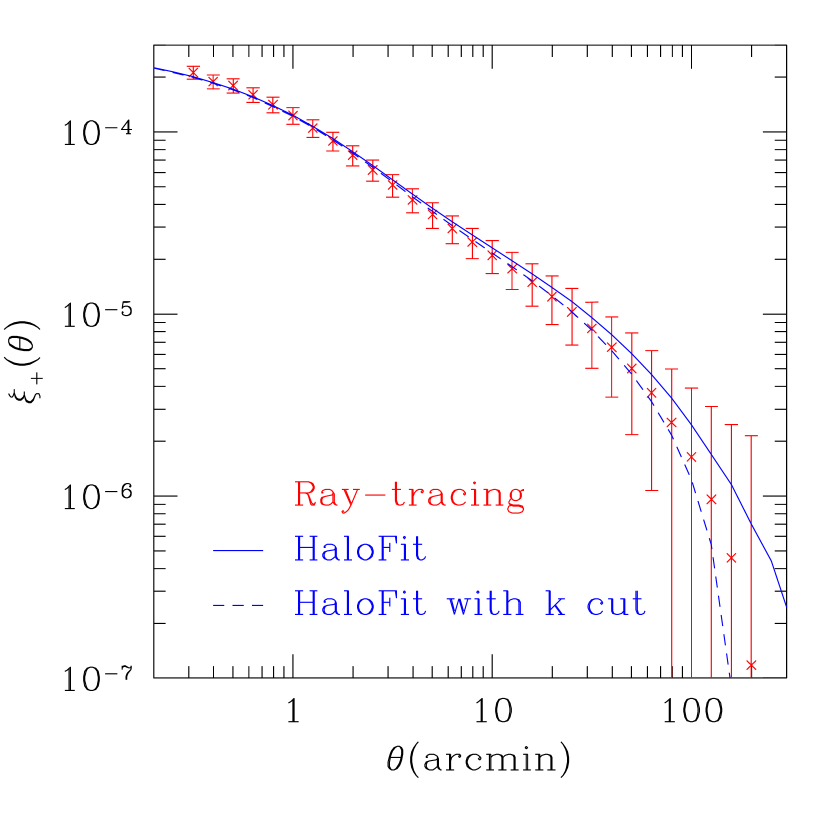
Figure 1.— The cosmic shear correlation function, $\xi_{+}(\theta)$ (see Eq. 1) for source redshift $z_{s}=1.0$, measured from our 1000 ray-tracing simulations. The error bars at each bin are estimated from the scatters ($1\sigma$ scatters) in the measured correlation functions of 1000 simulations. Note that each realization has an area of 25 square degrees, therefore the error bars show the sampling variance for the area coverage. For comparison the solid and dashed curves show the analytic predictions computed using HaloFit. The difference between the two curves is that the dashed curve includes only the contributions of mass density fluctuations with length scales within the box size of simulations (see text for details). The dashed curve is in better agreement with the simulation result over a wide range of separation angles.

Next we move on to the covariance matrix of shear correlation function. The covariance matrix describes how the correlation functions of different separation angles are correlated with each other. Following the methods developed in Joachimi et al. (2008) and Takada & Jain (2009), the covariance matrix for the correlation function $\xi_{+}(\theta)$ is expressed as

$${\rm Cov}[\xi_{+}(\theta),\xi_{+}(\theta^{\prime})]=\frac{1}{\pi\Omega_{\rm s}}\int_{0}^{\infty}l{\rm d}lJ_{0}(l\theta)J_{0}(l\theta^{\prime})P_{\kappa}(l)^{2}$$

$$+\frac{1}{4\pi^{2}\Omega_{\rm s}}\int_{0}^{\infty}l{\rm d}l\int_{0}^{\infty}l^{\prime}{\rm d}l^{\prime}J_{0}(l\theta)J_{0}(l^{\prime}\theta^{\prime})\bar{T}_{\kappa}(l,l^{\prime}),$$ (4)

where $\Omega_{\rm s}$ denotes the survey area and $\bar{T}_{\kappa}$ denotes the angle averaged lensing trispectrum. Note that we ignored the shot noise contribution due to random intrinsic ellipticities. The derivation of Eq. (4) assumes an ideal survey geometry; in other words Eq. (4) is approximately validated only for the case, $\theta,\theta^{\prime}\ll\sqrt{\Omega_{\rm s}}$ and for large area surveys such as $\Omega_{\rm s}\lower 2.15277pt\hbox{$\;\buildrel>\over{\sim}\;$}1000$ deg², as discussed in Appendix A in detail. Therefore it is expected that for a small survey area the covariance matrix deviates from the formula above. We will call it the finite area effect which is examined in Appendix A. See Joachimi et al. (2008) for expressions of other covariance matrices ${\rm Cov}[\xi_{-}(\theta),\xi_{-}(\theta^{\prime})]$ and ${\rm Cov}[\xi_{+}(\theta),\xi_{-}(\theta^{\prime})]$, which are examined in § 3.2.

The first term in Eq. (4) describes the Gaussian contribution, while the second term is the non-Gaussian contribution. There is an important difference between the covariance of the convergence power spectrum and that of the real-space correlation function. Even for a pure Gaussian field, the first term in Eq. (4) is non-vanishing for the off-diagonal components with $\theta\neq\theta^{\prime}$. The correlation functions of different separations are always correlated with each other. Also note that the covariance does not depend on the bin width of angles. Thus, when using the correlation function measurements for constraining cosmological parameters, it is very important to have an accurate model of the covariance matrix in order to properly interpret the measurement. We will use Eq. (4) to compare the analytical prediction with the covariance measured from the simulations.

2.2. Constructing a Gaussian Field from the Simulations

The main goal of this paper is to quantify the relative importance of the non-Gaussian covariance to the Gaussian covariance as a function of angular scales and source redshifts. To address this, we first construct a Gaussian field using the ray-tracing simulations in order to separate out the Gaussian covariance contribution. We will hereafter call the constructed maps “the simulated Gaussian fields”. The reason why we use the simulated Gaussian fields instead of using the analytical prediction (the first term of Eq. 4) is as follows. Firstly, the ray-tracing simulations do not include large-scale modes beyond the simulation box size. Secondly, as we will show below in detail, the covariance measured from the Gaussian simulations shows a nontrivial dependence on the survey area that cannot be fully described by the first term of Eq. (4).

We generated the Gaussian simulations according to the procedures below. Firstly, we Fourier-transformed each convergence field of 1000 ray-tracing simulations. Secondly, we make a Gaussian field by randomly selecting each Fourier mode from the Fourier coefficients of 1000 realizations, and then perform the inverse Fourier transform to obtain the real-space shear field imposing that the chosen Fourier modes satisfy the real number condition. Repeating this procedure, we made 1000 realizations of the Gaussian field. The simulated Gaussian fields generated in this way have the same power spectrum on average as that of the original simulations, and contain Fourier modes over the same range of angular scales as in the original simulations.

A justification of the Gaussian fields is given in Fig. 2, which shows the diagonal terms of power spectrum covariance matrix, measured from the original and Gaussian simulated maps, as a function of multipoles. The simulation results are plotted relative to the expectation for a Gaussian field, where the Gaussian covariance is equal to the squared power spectrum divided by the number of Fourier modes that are confined in each multipole bin. Therefore the deviations from unity arise from the non-Gaussian error contributions. The figure explicitly shows that, while the original simulations display stronger non-Gaussian covariances with increasing multipoles, the Gaussian simulations are consistent with the Gaussian expectation over a range of multipoles we consider.

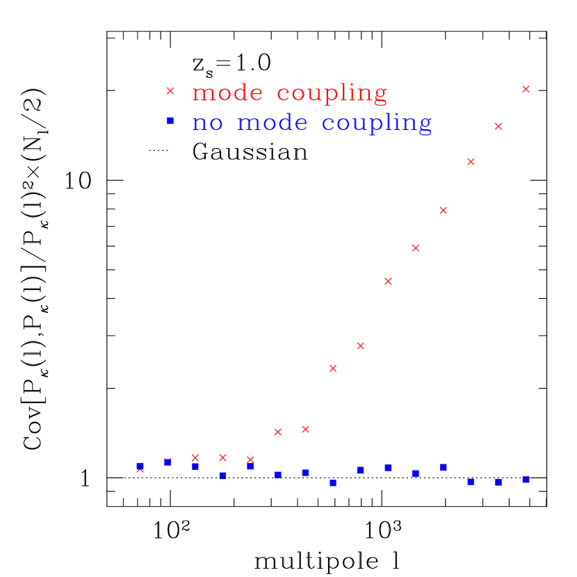
Figure 2.— The diagonal components of the convergence power spectrum covariance, divided by the expected Gaussian covariance (e.g. see, Sato et al., 2009), as a function of multipoles. The deviations from unity arise from the non-Gaussian errors. Note that the source redshift is $z_{s}=1.0$. The cross symbols are the simulation results from 1000 realizations, while the square symbols are the results obtained from the Gaussian simulations we generated from the 1000 simulations (see § 2.2). The Gaussian simulation results are consistent with unity over a range of multipoles.

Another justification is given in Fig. 3. The figure shows the probability distributions of convergence $\kappa$ for one realization of the original ray-tracing simulations (red histogram) and the Gaussianized realization (blue histogram), respectively. The results are for source redshift $z_{s}=1.0$. The original simulation, which includes the non-Gaussian contribution, shows a skewed distribution, which strongly deviates from the Gaussian distribution with the same variance width. The distribution is better described by a log-normal distribution (dashed curve), as studied in Taruya et al. (2002), but shows a larger positive tail. On the other hand, the Gaussian simulation is in good agreement with the Gaussian distribution (dotted curve).

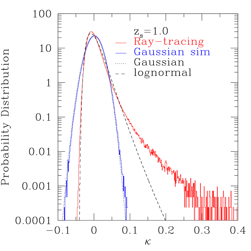
Figure 3.— The probability distributions of convergence $\kappa$ computed from the original ray-tracing simulation and the Gaussianized simulation, respectively (taken from one realization of each simulations). The Gaussian simulation result is consistent with the Gaussian distribution that has zero mean and the same variance as that measured from the simulation.

3. Results: calibrating the non-Gaussian covariances

3.1. Diagonal and Off-Diagonal Components of the Covariance Matrix

In this section we study the covariance matrix of shear correlation function using 1000 ray-tracing simulations.

The symbols in Fig. 4 show the diagonal components of the covariance matrix measured from 1000 simulations, for different source redshifts $z_{s}=0.6,1.0$ and 3.0, respectively. Again notice that each simulation realization has an area of 25 square degrees, so the plot shows the covariance expected when measuring the cosmic shear correlation from a survey with square-shaped survey geometry and 25 square degrees. Here we ignored the intrinsic ellipticity noise (we will come back to this later). First of all, we should stress that, by using the 1000 realizations (25000 square degrees in total), we can obtain well-converged measurements of the covariance elements over a range of the scales we consider. To be more quantitative, as shown in Appendix in Takahashi et al. (2011), covariances of the diagonal covariance elements scale approximately as $(2/N_{\rm r})^{1/2}$, where $N_{\rm r}$ is the number of simulation realizations. Therefore the covariance elements are measured to 4%-level accuracies.

We first compare the simulation results with the Gaussian error expectations (short-dashed curve) computed from the first term of Eq. (4). Note that we included only the Fourier modes confined within our simulations in the covariance calculation; we imposed $P_{\delta}(k)=0$ at $k<k_{\rm f}$ as done in Fig. 1. Contrary to the result in Fig. 1, the Gaussian predictions with the $k$-cutoff effect appear to overestimate the simulation results on large separation angles, where the non-Gaussian errors are insignificant. On the other hands, the dotted curves show the results obtained from the Gaussian simulations we constructed (see § 2.2), showing a good agreement with the simulation results on the large scales. Hence we conclude that the analytical prediction given by Eq. (4) is not sufficiently accurate over the scales we consider. In fact, as studied in detail in Appendix A, Eq. (4) can be valid only when the survey area is sufficiently large, such as 1000 square degrees. In Appendix A we develop an empirical model to compute the Gaussian covariance taking into account the finite survey area effect. The long-dashed curve shows the modified analytical prediction for the Gaussian covariance, which is computed using Eq. (A10) as well as including the $k$-cutoff for $P_{\delta}(k)$. The figure clearly shows that the modified analytical prediction well matches the Gaussian simulation results. Thus we need to properly account for both the finite range of Fourier modes and the finite survey area effect in order to obtain an accurate prediction of the covariance at large separations.

The simulation results (symbols) start to deviate from the Gaussian simulation results on small separation angles due to the non-Gaussian error contribution. The plot shows that the non-Gaussian errors are more significant on smaller angles and for lower source redshifts, because of stronger nonlinear clustering in structure formation at lower redshifts and on smaller length scales. For comparison, the solid curves show the halo model prediction developed in our previous paper (Sato et al., 2009). To be more precise, the halo model is used to compute the non-Gaussian covariance for the assumed cosmological model, including the “halo sampling variance term” (Sato et al., 2009) in addition to the non-Gaussian term (1-halo term). Then the solid curves are the sum of the halo-model-computed non-Gaussian covariance and the Gaussian covariance that is computed from the Gaussian simulations. The halo model predictions qualitatively well reproduce the simulation results on small separations as well as the source-redshift dependence. However, the halo model also shows a sizable disagreement due to the limitation.

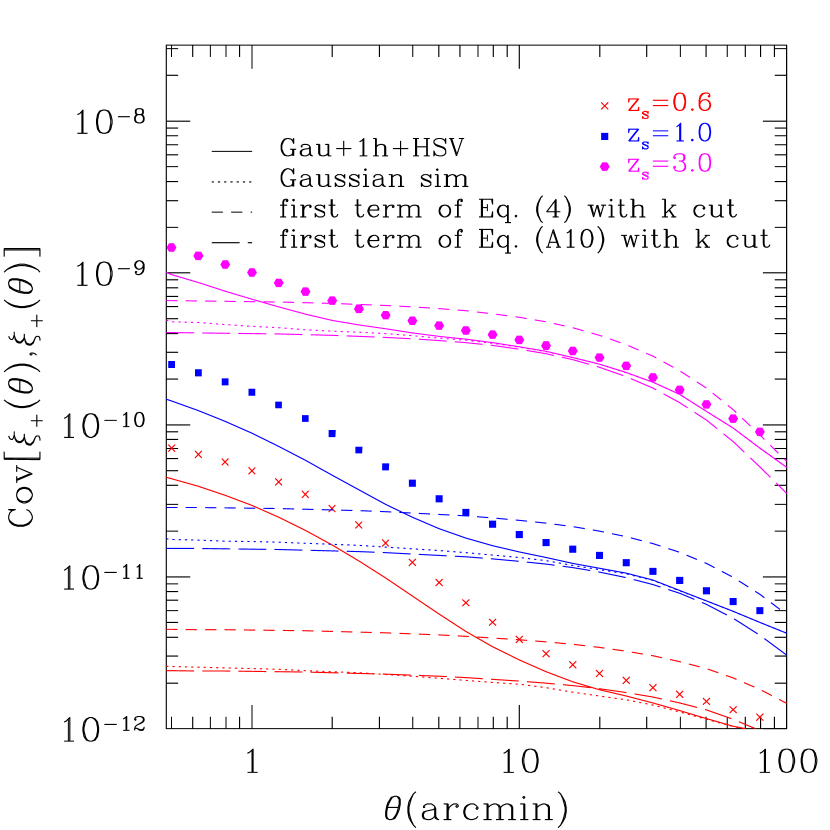
Figure 4.— The diagonal components of the covariance matrix of shear correlation function for different source redshifts, $z_{s}=0.6,1.0$ and 3.0. The cross, square and circle symbols are the simulation results from 1000 realizations for each source redshifts. The solid curves show the halo model predictions including the 1-halo term and the halo sample variance (see Sato et al., 2009, for the details). The dotted curves are the results obtained from the Gaussian simulations (see § 2.2 and Fig. 2). The short-dashed curves show the analytical predictions computed from the first term of Eq. (4), where we included only the Fourier modes contained within our simulation boxes, i.e. imposed the condition $P_{\delta}(k)=0$ at $k<k_{\rm f}$ in the covariance calculation as in Fig. 1. On the other hand, the long-dashed curves are the results which are computed using an empirical model to account for the finite survey area effect (see Appendix A for details). This modified Gaussian prediction better matches the Gaussian simulation results.

Fig. 5 shows the covariance matrices comparing the results for the original ray-tracing simulations, the Gaussian simulations and the Gaussian prediction computed from the first term of Eq. (4), where the $k$-cutoff and the finite survey area effect are included. Note that all the results are for $z_{s}=1$. The Gaussian prediction (right panel) and the Gaussian simulation results show a nice agreement for the scale-dependences and amplitudes. The original simulation results show totally different scale-dependences from the Gaussian results and display greater amplitudes at smaller separation angles (left-lower corner) due to stronger non-Gaussian contributions.

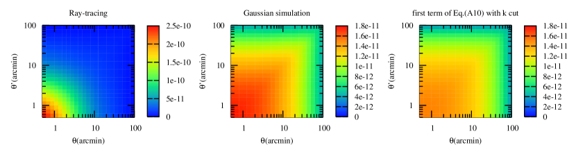
Figure 5.— The covariance matrices ${\rm Cov[\xi_{+}(\theta),\xi_{+}(\theta^{\prime})]}$ as a function of separation angles $\theta$ and $\theta^{\prime}$, for the ray-tracing simulation realization (left panel), the Gaussian simulation (middle) and the analytical prediction computed from the first term of Eq. (4) (right), respectively. All the results are for source redshift $z_{s}=1.0$. For the analytical Gaussian covariance, we included the finite survey area effect as well as the $k$-cutoff in the power spectrum calculation, as in Fig. 4.

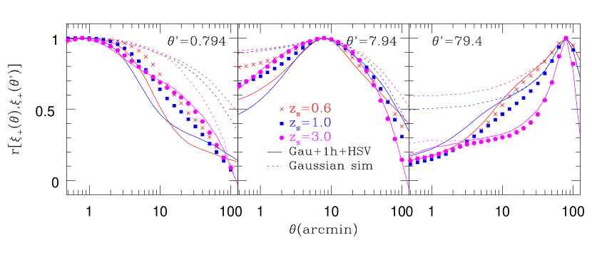
Figure 6.— The correlation coefficients $r[\xi_{+}(\theta),\xi_{+}(\theta^{\prime})]$ as a function of separation angles $\theta$, where $\theta^{\prime}$ is kept fixed to $\theta^{\prime}=0.794$, 7.94 and 79.4 (arcmin) in the left, middle and right panels, respectively. In each panel we show the results for different redshifts, $z_{s}=0.6,1.0$ and 3.0. The solid curves denote the halo model predictions, while the dotted curves denote the Gaussian error predictions.

Next we study the correlation coefficients to quantify strengths of the off-diagonal covariance components relative to the diagonal components:

$$r[\xi_{+}(\theta),\xi_{+}(\theta^{\prime})]\equiv\frac{{\rm Cov}[\xi_{+}(\theta),\xi_{+}(\theta^{\prime})]}{\sqrt{{\rm Cov}[\xi_{+}(\theta),\xi_{+}(\theta)]{\rm Cov}[\xi_{+}(\theta^{\prime}),\xi_{+}(\theta^{\prime})]}}.$$ (5)

The correlation coefficient is defined so that $r=1$ for the diagonal components when $\theta=\theta^{\prime}$. For off-diagonal components when $\theta\neq\theta^{\prime}$, $r\rightarrow 1$ implies strong correlation between the two correlation functions of different angular scales, while $r\rightarrow 0$ means no correlation.

Fig. 6 shows the correlation coefficients $r[\xi_{+}(\theta),\xi_{+}(\theta^{\prime})]$. There are significant correlations between different separation angles. Comparing the dotted and solid curves manifests less significant cross-correlations in the non-Gaussian errors than in the Gaussian errors, implying that the non-Gaussian errors preferentially contribute to the diagonal components.

3.2. A Fitting Formula of the Non-Gaussian Covariance Elements

By using the simulation results shown up to the preceding section we derive a fitting formula to compute the non-Gaussian covariance as a function of separation angles and source redshifts. To do this we employ the method developed in Semboloni et al. (2007), which is to derive the calibration function that gives the non-Gaussian covariance contribution relative to the Gaussian covariance. Our results bring several improvements over the results in Semboloni et al. (2007). Firstly, we use 1000 ray-tracing realizations, for each source redshift ($z_{s}=0.6,0.8,1.0,1.5,2.0,3.0$). Secondly, we carefully estimated the Gaussian covariance contribution using the Gaussian simulations (see § 2.2), thereby enabling us to reliably estimate the relative contribution of the non-Gaussian covariance.

We define $F(\theta,\theta^{\prime};z_{s})$, the ratio of the non-Gaussian covariance relative to the Gaussian expectation for the covariance matrix:

$$F(\theta,\theta^{\prime};z_{s})\equiv\frac{{\rm Cov_{\rm NG}}[\xi_{+}(\theta),\xi_{+}(\theta^{\prime});z_{s}]}{{\rm Cov_{\rm G}}[\xi_{+}(\theta),\xi_{+}(\theta^{\prime});z_{s}]}.$$ (6)

Here we used the 1000 simulations to compute the Gaussian and non-Gaussian covariance matrices appearing in the numerator and denominator of the above equation. As shown in Figs. 4 and 5 the non-Gaussian contributions are important only on small separation angles, $\lower 2.15277pt\hbox{$\;\buildrel<\over{\sim}\;$}10$ arcmin, for a $\Lambda$CDM cosmology and for source redshifts we consider.

Fig. 7 shows the simulation results for the diagonal components of $F(\theta,\theta^{\prime})$ for different source redshifts. The fitting formula for $F(\theta,\theta^{\prime})$ is given in Appendix B. The figure shows that all the curves go to unity, $F(\theta,\theta)=1$, on very large separations as expected; the non-Gaussian covariances become negligible on such large separations. This can be contrasted to the results in Semboloni et al. (2007) (see Fig. 1 in their paper), where the corresponding curves do not go to unity, even go below unity at large separations. This is because we carefully computed the Gaussian covariance contribution (see § 2.2), while Semboloni et al. (2007) used the analytical prediction (the first term of Eq. 4) to estimate the Gaussian covariance, which turns out to overestimate the simulation results. Also note that in Semboloni et al. (2007) all the Fourier modes setting the lower bound to $k=0$ or $l=0$ are included in the Gaussian covariance calculation (Eq. 4).

The figure also shows that the non-Gaussian errors are significant on smaller separations and for lower source redshifts, where nonlinear clustering is more evolving. For a source redshift $z_{s}\sim 1$, which is a typical depth of the Subaru-type survey, $F\lower 2.15277pt\hbox{$\;\buildrel>\over{\sim}\;$}10$ on scales smaller than 1 arcminutes, meaning that the non-Gaussian contribution to the diagonal covariance is greater than the Gaussian contribution by more than a factor of 10. The non-Gaussian covariance amplitudes are by accident similar to what is found in Semboloni et al. (2007), even though the power spectrum normalization $\sigma_{8}$ is quite different: $\sigma_{8}=0.76$ in our simulations, while $\sigma_{8}=1$ in Semboloni et al. (2007). Again this is subscribed to the fact that Semboloni et al. (2007) under-estimated the non-Gaussian error contribution. The normalization $\sigma_{8}=0.76$ we assumed is slightly lower than the currently most-favored value, $\sigma_{8}=0.8$ (see WMAP 7-year result, Komatsu et al., 2011). Therefore the fitting function $F(\theta,\theta^{\prime})$ we calibrated may slightly underestimate the non-Gaussian errors (by about 20%). To correct for this, we can use the halo model prediction to estimate the difference in the non-Gaussian covariance amplitudes for different $\sigma_{8}$ values, and then multiply the correction factor with $F(\theta,\theta^{\prime})$.

Let us summarize how to obtain the covariance matrix for given survey parameters from our fitting formula:

• Compute the first term of Eq. (A10) to estimate the Gaussian covariance matrix, for given survey area and source redshift.

• Use the fitting function Eq. (B1) for $F(\theta,\theta^{\prime};z_{s})$ to obtain the non-Gaussian covariance contribution.

• Multiply the quantities in the steps 1 and 2 to obtain the total covariance matrix.

Exactly speaking, the survey-area dependence of the non-Gaussian covariance is not as naively expected; ${\rm Cov}\propto 1/\Omega_{\rm s}$ does not hold due to the halo sampling variance contribution (Sato et al., 2009). However we have found that the residual dependence is relatively small, and our fitting formula for the covariance matrix is approximately valid for a survey area we are most interested in ($\;\buildrel>\over{\sim}\;$100 deg²).

While we have so far ignored the intrinsic ellipticity contribution to the covariance, we need to further include the effect. First of all, the intrinsic ellipticity noise contributes only to the Gaussian covariance, and does not affect the non-Gaussian covariance, as long as the intrinsic ellipticity alignment can be ignored. Hence we can easily include the shot noise contribution as follows.

One method is a simulation based method. We can generate the Gaussian field including the shot noise contribution by replacing the power spectrum $P_{\kappa}(l)$ with $P_{\kappa}(l)+\sigma_{\epsilon}^{2}/\bar{n}_{\rm g}$ in generating the simulation field, where $\sigma_{\epsilon}$ is the rms intrinsic ellipticity per component and $\bar{n}_{g}$ is the mean number density of source galaxies. Here we need to assume $\sigma_{\epsilon}$ and $\bar{n}_{g}$ that we measure from galaxies in a given survey. If we measure the covariance matrix from the Gaussian simulations generated in this way, the covariance matrix includes the contribution arising from the term $\propto(\sigma_{\epsilon}^{2}/\bar{n}_{g})^{2}$ as well as the mixed term between the cosmological Gaussian field and the shot noise term arising from the term $\propto P_{\kappa}(l)\sigma_{\epsilon}^{2}/\bar{n}_{g}$ (Schneider et al., 2002; Joachimi et al., 2008).

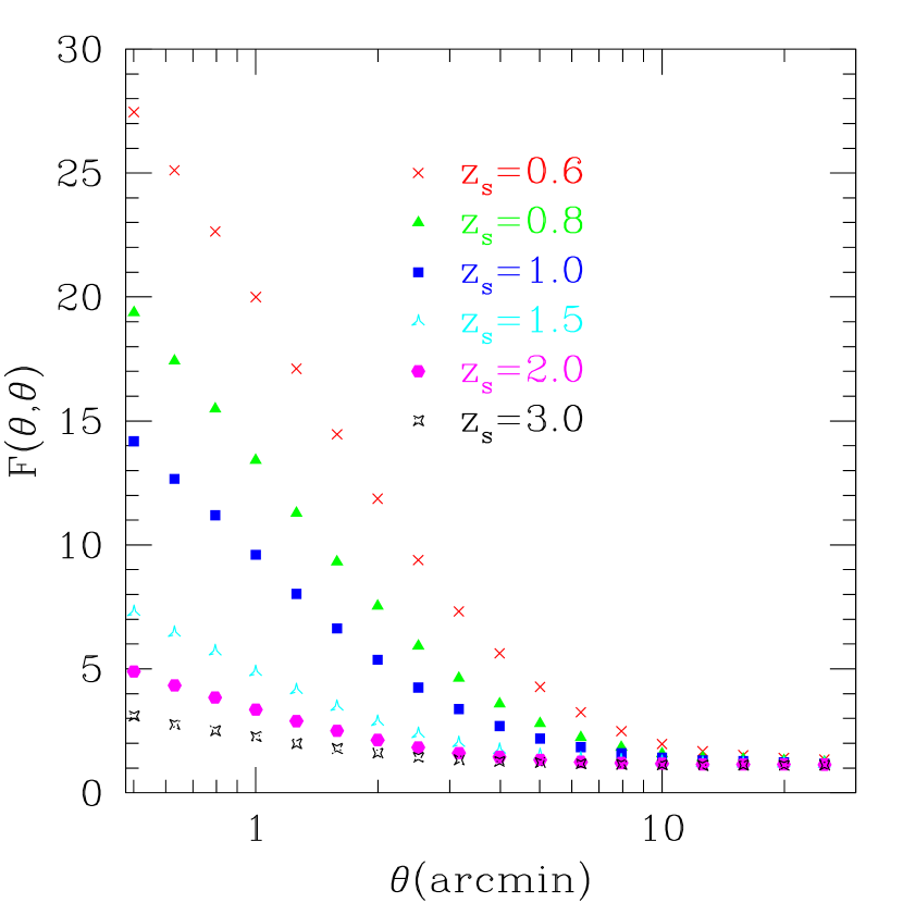
Figure 7.— The diagonal elements of shear correlation covariance relative to the Gaussian covariance contribution, as a function of separation angles and source redshifts (see Eq. 6 for the definition). The results are measured from the 1000 realizations, where the Gaussian contributions are estimated from the 1000 Gaussian simulations as in Fig. 2.

Another way is following the method in Joachimi et al. (2008) (also see Schneider et al., 2002), which developed an analytical formula of the Gaussian covariances including the intrinsic ellipticity noise contribution. To be more explicit, the formula is given in terms of the convergence power spectrum $P_{\kappa}(l)$, as in the first term of Eq. (4). Then the intrinsic noise contribution can be incorporated by replacing $P_{\kappa}(l)^{2}$ with $(P_{\kappa}(l)+\sigma_{\epsilon}^{2}/\bar{n}_{g})^{2}$. Here we need to assume $\sigma_{\epsilon}$ and $\bar{n}_{g}$ that are measured from a given survey.

Finally we comment on other contributions to the covariance matrix we have so far ignored, which are the covariance contributions arising from another shear correlation function $\xi_{-}(\theta)$: ${\rm Cov}[\xi_{-}(\theta),\xi_{-}(\theta^{\prime})]$ and ${\rm Cov}[\xi_{+}(\theta),\xi_{-}(\theta^{\prime})]$. Fig. 8 shows the results. Again the non-Gaussian error contributions are significant at scales $\lower 2.15277pt\hbox{$\;\buildrel<\over{\sim}\;$}10^{\prime}$. Compared to Fig. 4, the covariance matrices ${\rm Cov}[\xi_{-}(\theta),\xi_{-}(\theta^{\prime})]$ and ${\rm Cov}[\xi_{+}(\theta),\xi_{-}(\theta^{\prime})]$ have smaller amplitudes than ${\rm Cov}[\xi_{+}(\theta),\xi_{+}(\theta^{\prime})]$ does: for example, the amplitudes of ${\rm Cov}[\xi_{-}(\theta),\xi_{-}(\theta^{\prime})]$ and ${\rm Cov}[\xi_{+}(\theta),\xi_{-}(\theta^{\prime})]$ are smaller than that of ${\rm Cov}[\xi_{+}(\theta),\xi_{+}(\theta^{\prime})]$ by a factor of 100 and 10, respectively. However, the genuine effects need to be understood in terms of the signal-to-noise ratios that are roughly estimated as $\xi_{+}^{2}/{\rm Cov}[\xi_{+},\xi_{+}]$ or $\xi_{+}\xi_{-}/{\rm Cov}[\xi_{+},\xi_{-}]$ at each separation angles. Since the correlation function $\xi_{-}$ has smaller amplitudes than $\xi_{+}$ does, by a factor of 10 at separations $\sim 1^{\prime}$ (e.g. see Fig. 2 in Schneider et al., 2002), therefore the covariances ${\rm Cov}[\xi_{-}(\theta),\xi_{-}(\theta^{\prime})]$ and ${\rm Cov}[\xi_{+}(\theta),\xi_{-}(\theta^{\prime})]$ are not negligible.

We tried to derive fitting formulas for the non-Gaussian covariance contributions to ${\rm Cov}[\xi_{-}(\theta),\xi_{-}(\theta^{\prime})]$ and ${\rm Cov}[\xi_{+}(\theta),\xi_{-}(\theta^{\prime})]$ in the similar manner as done in Eq. (6). However, due to complex scale-dependences of the Gaussian covariances as implied in Fig. 8, we could not find useful fitting formulas that are expressed by simple analytical functions. Therefore, the covariance matrix contributions need to be directly calibrated from the ray-tracing simulations. The table-format covariances for ${\rm Cov}[\xi_{-}(\theta),\xi_{-}(\theta^{\prime})]$ and ${\rm Cov}[\xi_{+}(\theta),\xi_{-}(\theta^{\prime})]$ are available upon request.

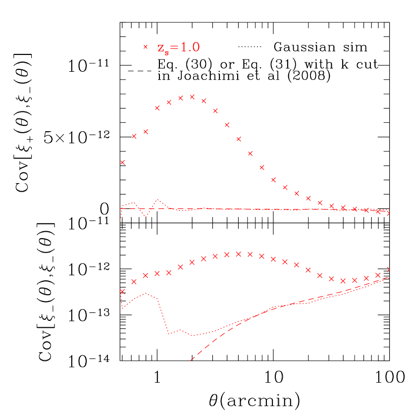
Figure 8.— The diagonal components of shear correlation covariances ${\rm Cov}[\xi_{-}(\theta),\xi_{-}(\theta^{\prime})]$ and ${\rm Cov}[\xi_{+}(\theta),\xi_{-}(\theta^{\prime})]$ as a function of separation angles at source redshift $z_{s}=1.0$. The cross symbols are the simulation results measured from the 1000 realizations. The dotted curves are the results obtained from the Gaussian simulations (see § 2.2), while the dashed curves the theoretical predictions computed from Eq. (30) or Eq. (31) in Joachimi et al. (2008), where we included the $k$-cutoff in the lensing power spectrum calculation.

4. Conclusion

In this paper, we have developed the theoretical model of the covariance matrix of cosmic shear two-point correlation function taking into account the effect of finite survey area and the effects of non-linear gravitational clustering in large-scale structure.

We found that the survey-area dependence of the Gaussian covariance, which scales as $\propto 1/\Omega_{\rm s}$ in the commonly used formula, does not hold for a small area survey due to the effect of finite survey area. The conventional formula is valid only when the survey area is sufficiently wide such as 1000 square degrees. We examined the residual survey-area dependence using the method developed by Schneider et al. (2002), and obtained an empirical formula which reproduces our results.

We examined the non-Gaussian covariance as a function of angular scales and source redshifts by using two sets of simulation data: (1) the ray-tracing simulations for the standard $\Lambda$CDM cosmology and (2) Gaussian fields which have the same power spectrum on average as that of the original simulations. The non-Gaussian errors become more significant on smaller scales and at lower redshifts. We compared the simulation results with halo model predictions and found that the halo model qualitatively well reproduces the non-Gaussian error over a wide range of separation angles and for redshifts we have considered. However, the halo model also displays sizable disagreement with the simulation results.

Following Semboloni et al. (2007), we derived the calibration function to compute the non-Gaussian covariance contribution relative to the Gaussian covariance (Eq. 6). The Gaussian field data allows us to cleanly separate out the Gaussian covariance contribution accurately, thereby enabling us to reliably estimate the calibration function. We found that the calibration factor at arcminute scales can be high as $\sim$ 20 and $\sim$ 10 for source redshifts of $z_{s}=0.6$ and $1.0$, respectively. The transition between Gaussian and non-Gaussian covariance occurs around 10 and 5 arcminute for $z_{s}=0.6$ and 1.0, respectively. Therefore, when one derives constrains on the cosmological parameters from cosmic shear correlation measurements, it is important to properly account for the non-Gaussian effects. The fitting formulae, Eq. (A10) and Eq. (B1), developed in this paper allow one to compute the covariance matrix including the non-Gaussian contribution for given survey parameters (the survey area and the source redshift).

Simulation data (1000 convergence power spectra and cosmic shear correlation functions for $\xi_{+}(\theta)$ and $\xi_{-}(\theta)$.) are available upon request (contact masanori@a.phys.nagoya-u.ac.jp).

Appendix A Finite Area Effect of the Gaussian Covariance

In this section, we study the validity of the first term of Eq. (4), which gives the Gaussian error prediction for the shear correlation function covariance, and will show the prediction is only valid for a large-area survey covering more than $1000$ square degrees. For this purpose we will use the method developed in Schneider et al. (2002).

Let us begin with considering an estimator of the shear correlation function of a separation angle $\theta$, $\hat{\xi}_{+}(\theta)$. For a given galaxy catalog the shear correlation function can be estimated as

$$\hat{\xi}_{+}(\theta)\equiv\frac{1}{N_{\rm pair}}\sum_{i}\sum_{j}\left(\epsilon_{t(i)}\epsilon_{t(j)}+\epsilon_{\times(i)}\epsilon_{\times(j)}\right)\Delta(|\bm{\theta}_{i}-\bm{\theta}_{j}|;\theta),$$ (A1)

where we have used the abbreviated notations such as $\epsilon_{t(i)}$ to denote the ellipticity component of the $i$-th galaxy at the angular position $\bm{\theta}_{i}$, $N_{\rm pair}$ is the total number of pairs of galaxies that are separated by the separation angle $\theta$ and the index $i$ in summation runs over all the galaxies in the catalog. The tangential and cross components of the ellipticity $\epsilon=\epsilon_{1}+{\rm i}\epsilon_{2}$ at position $\bm{\vartheta}$ are defined as

$$\epsilon_{t}=-\mathcal{R}e\left(\epsilon\,e^{-2{\rm i}\varphi}\right);\qquad\qquad\epsilon_{\times}=-\mathcal{I}m\left(\epsilon\,e^{-2{\rm i}\varphi}\right),$$ (A2)

where $\mathcal{R}e$ and $\mathcal{I}m$ denote the real- and imaginary-parts of the quantities and $\varphi$ is the polar angle of the separation vector between two galaxies, $\bm{\theta}$. The component, $\epsilon_{t}$, is defined as the ellipticity component in parallel or perpendicular direction relative to the line connecting the two galaxies. On the other hand $\epsilon_{\times}$ are measured from the $\pm 45^{\circ}$ rotated components. The function $\Delta(|\bm{\theta}_{i}-\bm{\theta}_{j}|;\theta)$ is a selection function defined in that $\Delta(|\bm{\theta}_{i}-\bm{\theta}_{j}|;\theta)=1$ if $\theta-\delta\theta/2\leq|\bm{\theta}_{i}-\bm{\theta}_{j}|\leq\theta+\delta\theta/2$, otherwise $\Delta(|\bm{\theta}_{i}-\bm{\theta}_{j}|;\theta)=0$, where $\delta\theta$ is the bin width of separation angle. The total number of galaxy pairs is given as $N_{\rm pair}=\sum_{ij}\Delta(|\bm{\theta}_{i}-\bm{\theta}_{j}|;\theta)$. The ensemble average of the estimator Eq. (A1) is found to indeed give the shear correlation function:

$$\langle\hat{\xi}_{+}(\theta)\rangle=\frac{1}{N_{\rm pair}}\sum_{ij}\langle\epsilon_{t(i)}\epsilon_{t(j)}+\epsilon_{\times(i)}\epsilon_{\times(j)}\rangle\Delta(|\bm{\theta}_{i}-\bm{\theta}_{j}|;\theta)=\frac{1}{N_{\rm pair}}\sum_{ij}\xi_{+}(|\bm{\theta}_{i}-\bm{\theta}_{j}|)\Delta(|\bm{\theta}_{i}-\bm{\theta}_{j}|;\theta)=\xi_{+}(\theta).$$ (A3)

Similarly the covariance is defined in terms of the estimator $\hat{\xi}_{+}(\theta)$ as

$${\rm Cov}[\xi_{+}(\theta),\xi_{+}(\theta^{\prime})]=\langle\hat{\xi}_{+}(\theta)\hat{\xi}_{+}(\theta^{\prime})\rangle-\xi_{+}(\theta)\xi_{+}(\theta^{\prime}).$$ (A4)

For simplicity, let us consider the diagonal parts of the covariance matrix, $\theta=\theta^{\prime}$. For the Gaussian field, the diagonal parts are computed as (Schneider et al., 2002):

$${\rm Cov}[\xi_{+}(\theta),\xi_{+}(\theta)]=\frac{1}{N_{\rm pair}^{2}}\sum_{ijlm}\langle\left(\epsilon_{t(i)}\epsilon_{t(j)}+\epsilon_{\times(i)}\epsilon_{\times(j)}\right)\left(\epsilon_{t(l)}\epsilon_{t(m)}+\epsilon_{\times(l)}\epsilon_{\times(m)}\right)\rangle\Delta(|\bm{\theta}_{i}-\bm{\theta}_{j}|;\theta)\Delta(|\bm{\theta}_{l}-\bm{\theta}_{m}|;\theta)-\xi_{+}(\theta)^{2}$$

$$=\frac{1}{N_{\rm pair}^{2}}\sum_{ijlm}[\xi_{+}(|\bm{\theta}_{i}-\bm{\theta}_{m}|)\xi_{+}(|\bm{\theta}_{j}-\bm{\theta}_{l}|)+\cos\left[4\left(\varphi_{im}-\varphi_{jl}\right)\right]\xi_{-}(|\bm{\theta}_{i}-\bm{\theta}_{m}|)\xi_{-}(|\bm{\theta}_{j}-\bm{\theta}_{l}|)]\Delta(|\bm{\theta}_{i}-\bm{\theta}_{j}|;\theta)\Delta(|\bm{\theta}_{l}-\bm{\theta}_{m}|;\theta)$$

$$\equiv\frac{1}{N_{\rm pair}^{2}}\sum_{ijlm}F_{ijlm},$$ (A5)

where $\varphi_{im}$ is the polar angle of the difference vector $\bm{\theta}_{i}-\bm{\theta}_{m}$, and we used the fact that an estimator for $\xi_{-}(\theta)$ is analogously defined as

$$\hat{\xi}_{-}(\theta)\equiv\frac{1}{N_{\rm pair}}\sum_{i}\sum_{j}\left(\epsilon_{t(i)}\epsilon_{t(j)}-\epsilon_{\times(i)}\epsilon_{\times(j)}\right)\Delta(|\bm{\theta}_{i}-\bm{\theta}_{j}|;\theta).$$ (A6)

Now we use Eq. (A5) to study the effect of finite survey area. This can be done by comparing the result with the first term of Eq. (4) because Eq. (4) ignores the survey geometry effect. To do this we performed the simplified test. Firstly, we randomly distribute galaxy positions with square shape geometry. Then, rather than working on the shear field in simulations, we will compute the summation in Eq. (A5) by using the tabulated data of $\xi_{+}(\theta)$ and $\xi_{-}(\theta)$. We estimate $\xi_{+}(\theta)$ and $\xi_{-}(\theta)$ using Eq. (1) and Eq. (2). In this case, the summation such as $\sum_{ij}$ runs over all the galaxies in the square-shaped mock simulation, and the separation angle such as $|\bm{\theta}_{i}-\bm{\theta}_{j}|$ can be exactly computed from the separation between the two galaxies chosen.

The symbols in Fig. 9 show the results of Eq. (A5) for the diagonal covariance matrix elements as a function of separation angles and mock simulation areas. The solid curves are the results computed from the first term of Eq. (4). In both cases we used the HaloFit prediction to compute the lensing power spectrum, which is then used to compute the shear correlation function as well as to compute the first term of Eq. (4). Note that we do not plot the symbols where separation angle becomes comparable with the scale of the mock simulation area due to avoid the boundary effect of the square-shaped mock simulation.

The figure clearly shows that the symbol is in good agreement with the solid curve for the largest area we consider, $\Omega_{\rm s}=3200$ deg², however, the two results disagree in amplitudes for the smaller areas, although the shape looks similar. In addition, comparing the results for $\Omega_{\rm s}=1.56$ and 25 deg² manifests that the disagreement is greater for the smaller survey area. This disagreement arises due to the effect of the finite survey area. Hence the conventionally used expression for the Gaussian covariance, the first term of Eq. (4), appears to overestimate the covariance amplitude. The formula is only valid for a sufficiently large area such as $\Omega_{\rm s}\lower 2.15277pt\hbox{$\;\buildrel>\over{\sim}\;$}1000$ deg². In other words, due to the finite survey area effect, the covariance of shear correlation function does not scale with survey area as ${\rm Cov}\propto 1/\Omega_{\rm s}$, which is assumed in the conventional formula (Eq. 4).

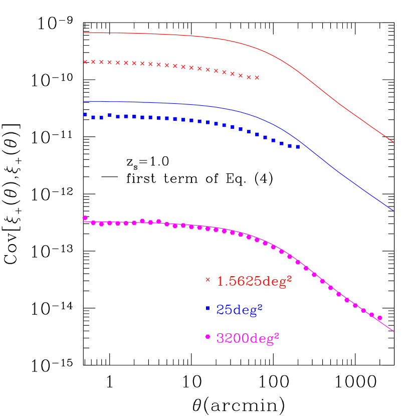
Figure 9.— A numerical test for studying the finite area effect on the Gaussian covariance of shear correlation (see text for the details). The symbols show the results for the diagonal covariance elements, which are computed using Eq. (A5), for different areas of square-shaped mock simulations: $\Omega_{\rm s}=1.5625$ ${\rm deg}^{2}$, 25 deg² and 3200 deg². The source redshift is $z_{s}=1.0$. The solid curves are the prediction computed from the first term of Eq. (4). The two results agree for a large area such as $\Omega_{\rm s}=3200$ deg², but disagree for the smaller areas probably due to the finite-area effect.

From now on, we will in more detail study how the difference between the results of Eqs. (4) and (A5) arises. Let us consider two survey areas A and B, assuming the area B is included in the area A (A $\supset$ B). By using Eq. (A5) the diagonal covariance matrix for a survey A can be expressed as

$${\rm Cov}_{\rm A}[\xi_{+}(\theta),\xi_{+}(\theta)] =\frac{1}{N_{\rm pair}^{2}\mid_{ijlm\in{\rm A}}}\left(\sum_{ijlm\in{\rm A-B}}\!\!F_{ijlm}+4\!\!\!\!\sum_{\begin{subarray}{c}i\in{\rm B}\\ \>{jlm}\in{\rm A-B}\end{subarray}}\!\!F_{ijlm}+2\!\!\!\!\sum_{\begin{subarray}{c}ij\in{\rm B}\\ \quad\!{lm}\in{\rm A-B}\end{subarray}}\!\!F_{ijlm}\right.$$

$$\left.+\>{2}\!\!\!\!\sum_{\begin{subarray}{c}\!\!{il}\in{\rm B}\\ \quad\!\!\!\!{jm}\in{\rm A-B}\end{subarray}}\!\!F_{ijlm}+2\!\!\!\!\sum_{\begin{subarray}{c}\!\!\!\!{im}\in{\rm B}\\ \quad{jl}\in{\rm A-B}\end{subarray}}\!\!F_{ijlm}+4\!\!\!\!\sum_{\begin{subarray}{c}{jlm}\in{\rm B}\quad\\ \quad\>{i}\in{\rm A-B}\end{subarray}}\!\!F_{ijlm}+\!\!\!\!\sum_{ijlm\in{\rm B}\quad}\!\!F_{ijlm}\right),$$ (A7)

where the notation $ij\in{\rm B}$ is introduced to mean that the indices $i$ and $j$ are included in B, and the notation $lm\in{\rm A-B}$ means that the indices $l$ and $m$ are included in the region that is in A, but not in B. We will consider the case that survey area A is sufficiently large in the following discussion. We define the value arising from finite area effect as

$${\rm FAE}\equiv\frac{\rm A}{\rm B}{\rm Cov}_{\rm A}[\xi_{+}(\theta),\xi_{+}(\theta)]-{\rm Cov}_{\rm B}[\xi_{+}(\theta),\xi_{+}(\theta)].$$ (A8)

If B is close to A, there is no finite area effect and FAE should be zero because of survey area as ${\rm Cov}\propto{1/\Omega_{\rm s}}$. If B is close to A, the final term of Eq. (A7) has a dominant contribution because the number of galaxy pairs is greater than other terms. In this case Eq. (A8) becomes

$${\rm FAE} \equiv\frac{\rm A}{\rm B}{\rm Cov}_{\rm A}[\xi_{+}(\theta),\xi_{+}(\theta)]-{\rm Cov}_{\rm B}[\xi_{+}(\theta),\xi_{+}(\theta)]\simeq\frac{\rm A}{\rm B}\frac{1}{N_{\rm pair}^{2}\mid_{ijlm\in{\rm A}}}\sum_{ijlm\in{\rm B}\quad}\!\!F_{ijlm}-{\rm Cov}_{\rm B}[\xi_{+}(\theta),\xi_{+}(\theta)]$$

$$\simeq\frac{1}{N_{\rm pair}^{2}\mid_{ijlm\in{\rm B}}}\sum_{ijlm\in{\rm B}\quad}\!\!F_{ijlm}-{\rm Cov}_{\rm B}[\xi_{+}(\theta),\xi_{+}(\theta)]=0.$$ (A9)

Thus Eq. (A8) has an asymptotic limit of ${\rm Cov}_{\rm A}={\rm Cov}_{\rm B}$ when ${\rm A}={\rm B}$. However, the other terms in Eq. (A7) are not negligible if ${\rm A}\neq{\rm B}$, and the covariances for a general case do not scale with survey area as ${\rm Cov}\propto 1/\Omega_{\rm s}$, due to a finite survey area effect.

Therefore we will estimate a fitting formula to account for the survey area dependence by assuming the form

$${\rm Cov}[\xi_{+}(\theta),\xi_{+}(\theta^{\prime})]=\frac{1}{\pi\Omega_{\rm s}f(\Omega_{\rm s})}\int_{0}^{\infty}l{\rm d}lJ_{0}(l\theta)J_{0}(l\theta^{\prime})P_{\kappa}(l)^{2}+\frac{1}{4\pi^{2}\Omega_{\rm s}f(\Omega_{\rm s})}\int_{0}^{\infty}l{\rm d}l\int_{0}^{\infty}l^{\prime}{\rm d}l^{\prime}J_{0}(l\theta)J_{0}(l^{\prime}\theta^{\prime})\bar{T}_{\kappa}(l,l^{\prime}),$$ (A10)

where $f(\Omega_{\rm s})$ denotes the new survey area dependence. We parametrize $f(\Omega_{\rm s})$ as

$$f(\Omega_{\rm s})=\frac{\alpha(z_{s})}{\Omega_{\rm s}^{\beta(z_{s})}}.$$ (A11)

We estimate the 2 parameters using the mock simulations as in Fig. 9, for different source redshifts $z_{s}=0.6,0.8,1.0,1.5,2.0$ and $3.0$. The mock simulation results are well fitted by the parameters

$$\alpha(z_{s})=\alpha_{1}z_{s}^{\alpha_{2}}$$

$$\beta(z_{s})=\beta_{1}z_{s}^{\beta_{2}}.$$ (A12)

The best-fitting parameters are found to be $(\alpha_{1},\alpha_{2})=(3.2952,-0.316369)$ and $(\beta_{1},\beta_{2})=(0.170708,-0.349913)$, respectively. As shown in Fig. 10 we made the fitting over survey areas of $1.5625\leq\Omega_{\rm s}\leq 1600$ deg² using the diagonal covariance at 50 arcmin. However we checked that the above fitting formula fairly well reproduce the results for different separations and for the off-diagonal covariance elements. A caution on the use of the fitting formula is the output value should be replaced to unity if the value is below unity.

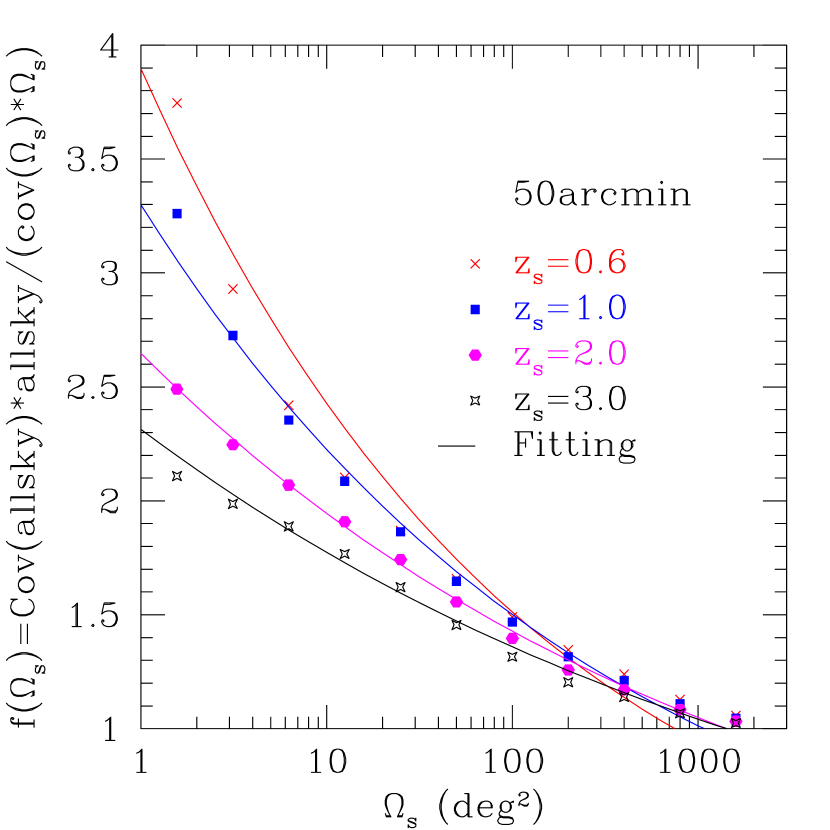
Figure 10.— A fitting formula for the survey area dependence of the Gaussian covariance, $f(\Omega_{\rm s})$ in Eq. (A10). The symbols are the mock simulation results for different source redshifts as in Fig. 9, and the solid curves are the fitting formula given by Eq. (A11). We did the fitting by matching to the mock simulation results for the diagonal Gaussian matrix at the scale of 50 arcmin.

Appendix B Fitting Formula for Calibration Matrix

In this section we estimate the calibration function $F(\theta,\theta;z_{s})$ we studied in § 3.2, which can be used to estimate the non-Gaussian covariance in combination with the fitting formula (A10) for the Gaussian covariance. We parametrize $F(\theta,\theta^{\prime};z_{s})$ as

$$F(\theta,\theta^{\prime};z_{s})=\left(a(z_{s})+\frac{b(z_{s})}{(\theta\theta^{\prime})^{c(z_{s})}}\right)\cdot d(z_{s})^{|\theta-\theta^{\prime}|}.$$ (B1)

The 4 parameters are estimated from the ray-tracing simulations for 6 different source redshifts $z_{s}=0.6,0.8,1.0,1.5,2.0$ and $3.0$. As demonstrated in Figs. 11 and 12, the simulation results are well fitted by the following best-fitting parameters:

$$a(z_{s})=-z_{s}^{a_{1}}\exp(a_{2}z_{s})+a_{3}$$

$$b(z_{s})=b_{1}z_{s}^{b_{2}}+b_{3}$$

$$c(z_{s})=c_{1}z_{s}^{c_{2}}+c_{3}$$

$$d(z_{s})=d_{1}z_{s}^{d_{2}}+d_{3},$$ (B2)

where $(a_{1},a_{2},a_{3})=(-3.7683,0.9752,1.4048)$, $(b_{1},b_{2},b_{3})=(10.7926,-2.0284,-0.2266)$, $(c_{1},c_{2},c_{3})=(-0.3664,-0.5733,0.6863)$, and $(d_{1},d_{2},d_{3})=(0.2450,0.1218,0.7076)$, respectively. We made this fitting over angular scales $0.5<\{\theta,\theta^{\prime}\}\leq$ 10 arcmin. Figs. 11 and 12 clearly show that the fitting formula above well reproduce the simulation results, and the accuracy of the fitting formula is within about 25%. However it should be noted that the fitting formula is only applied to source redshift ranges $0.6\leq z_{s}\leq 3.0$ and angular scales below 10 arcmin. This is sufficient because the non-Gaussian covariance is important only below 10 arcmin.

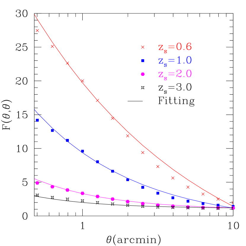
Figure 11.— The diagonal components of the calibration function to compute the non-Gaussian covariance, $F(\theta,\theta;z_{s})$ (see Eq. 6 for the definition). The symbols are the same as in Fig. 7, and the solid curves are the fitting formula given by Eq. (B1).

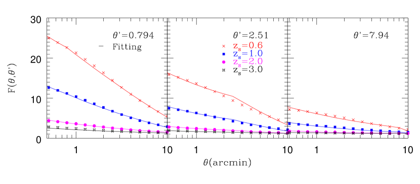
Figure 12.— As in the previous figure, but for the off-diagonal components. Shown is the function $F(\theta,\theta^{\prime})$ as a function of $\theta$, but $\theta^{\prime}$ is kept fixed to $\theta^{\prime}=0.794$, 2.51 and 7.94 (arcmin) in the left, middle and right panels, respectively.

References

- Albrecht et al. (2009) Albrecht, A., et al. 2009, arXiv:0901.0721
- Albrecht et al. (2006) Albrecht, A., et al. 2006, arXiv:astro-ph/0609591
- Bacon et al. (2000) Bacon, D. J., Refregier, A. R., & Ellis, R. S. 2000, MNRAS, 318, 625
- Bartelmann & Schneider (2001) Bartelmann, M., & Schneider, P. 2001, Phys. Rep., 340, 291
- Cooray & Hu (2001) Cooray, A., & Hu, W. 2001, ApJ, 554, 56
- Doré et al. (2009) Doré, O., Lu, T., & Pen, U.-L. 2009, arXiv:0905.0501
- Eifler et al. (2009) Eifler, T., Schneider, P., & Hartlap, J. 2009, A&A, 502, 721
- Eisenstein et al. (2005) Eisenstein, D. J., et al. 2005, ApJ, 633, 560
- Fu et al. (2008) Fu, L., et al. 2008, A&A, 479, 9
- Hamana et al. (2003) Hamana, T., et al. 2003, ApJ, 597, 98
- Hartlap et al. (2009) Hartlap, J., Schrabback, T., Simon, P., & Schneider, P. 2009, A&A, 504, 689
- Hicken et al. (2009) Hicken, M., Wood-Vasey, W. M., Blondin, S., Challis, P., Jha, S., Kelly, P. L., Rest, A., & Kirshner, R. P. 2009, ApJ, 700, 1097
- Hikage et al. (2011) Hikage, C., Takada, M., Hamana, T., & Spergel, D. 2011, MNRAS, 412, 65
- Hu (1999) Hu, W. 1999, ApJ, 522, L21
- Huterer (2002) Huterer, D. 2002, Phys. Rev. D, 65, 063001
- Ichiki et al. (2009) Ichiki, K., Takada, M., & Takahashi, T. 2009, Phys. Rev. D, 79, 023520
- Jarvis et al. (2006) Jarvis, M., Jain, B., Bernstein, G., & Dolney, D. 2006, ApJ, 644, 71
- Joachimi et al. (2008) Joachimi, B., Schneider, P., & Eifler, T. 2008, A&A, 477, 43
- Joudaki et al. (2009) Joudaki, S., Cooray, A., & Holz, D. E. 2009, Phys. Rev. D, 80, 023003
- Kaiser et al. (2000) Kaiser, N., Wilson, G., & Luppino, G. A. 2000, arXiv:astro-ph/0003338
- Komatsu et al. (2011) Komatsu, E., et al. 2011, ApJS, 192, 18
- Lu et al. (2010) Lu, T., Pen, U., & Doré, O. 2010, Phys. Rev. D, 81, 123015
- Mantz et al. (2010) Mantz, A., Allen, S. W., Rapetti, D., & Ebeling, H. 2010, MNRAS, 406, 1759
- Massey et al. (2005) Massey, R., Refregier, A., Bacon, D. J., Ellis, R., & Brown, M. L. 2005, MNRAS, 359, 1277
- Miyazaki et al. (2006) Miyazaki, S., et al. 2006, Proc. SPIE, 6269, 9
- Munshi et al. (2008) Munshi, D., Valageas, P., van Waerbeke, L., & Heavens, A. 2008, Phys. Rep., 462, 67
- Okumura et al. (2008) Okumura, T., Matsubara, T., Eisenstein, D. J., Kayo, I., Hikage, C., Szalay, A. S., & Schneider, D. P. 2008, ApJ, 676, 889
- Perlmutter et al. (1999) Perlmutter, S., et al. 1999, ApJ, 517, 565
- Pielorz et al. (2010) Pielorz, J., Rödiger, J., Tereno, I., & Schneider, P. 2010, A&A, 514, A79
- Refregier et al. (2010) Refregier, A., Amara, A., Kitching, T. D., Rassat, A., Scaramella, R., Weller, J., & Euclid Imaging Consortium, f. t. 2010, arXiv:1001.0061
- Riess et al. (1998) Riess, A. G., et al. 1998, AJ, 116, 1009
- Sato et al. (2009) Sato, M., Hamana, T., Takahashi, R., Takada, M., Yoshida, N., Matsubara, T., & Sugiyama, N. 2009, ApJ, 701, 945
- Sato et al. (2010) Sato, M., Ichiki, K., & Takeuchi, T. T. 2010, Physical Review Letters, 105, 251301
- Sato et al. (2011) Sato, M., Ichiki, K., & Takeuchi, T. T. 2011, Phys. Rev. D, 83, 023501
- Schneider et al. (2002) Schneider, P., van Waerbeke, L., Kilbinger, M., & Mellier, Y. 2002, A&A, 396, 1
- Schrabback et al. (2010) Schrabback, T., et al. 2010, A&A, 516, A63
- Semboloni et al. (2006) Semboloni, E., et al. 2006, A&A, 452, 51
- Semboloni et al. (2007) Semboloni, E., van Waerbeke, L., Heymans, C., Hamana, T., Colombi, S., White, M., & Mellier, Y. 2007, MNRAS, 375, L6
- Seo et al. (2011) Seo, H., Sato, M., Dodelson, S., Jain, B., & Takada, M. 2011, ApJ, 729, L11
- Smith et al. (2003) Smith, R. E., et al. 2003, MNRAS, 341, 1311
- Spergel et al. (2007) Spergel, D. N., et al. 2007, ApJS, 170, 377
- Takada & Jain (2004) Takada, M., & Jain, B. 2004, MNRAS, 348, 897
- Takada & Jain (2009) Takada, M., & Jain, B. 2009, MNRAS, 395, 2065
- Takahashi et al. (2011) Takahashi, R., et al. 2011, ApJ, 726, 7
- Taruya et al. (2002) Taruya, A., Takada, M., Hamana, T., Kayo, I., & Futamase, T. 2002, ApJ, 571, 638
- Van Waerbeke & Mellier (2003) Van Waerbeke, L., & Mellier, Y. 2003, arXiv:astro-ph/0305089
- Van Waerbeke et al. (2000) Van Waerbeke, L., et al. 2000, A&A, 358, 30
- Vikhlinin et al. (2009) Vikhlinin, A., et al. 2009, ApJ, 692, 1060
- White & Hu (2000) White, M., & Hu, W. 2000, ApJ, 537, 1
- Wittman et al. (2000) Wittman, D. M., Tyson, J. A., Kirkman, D., Dell’Antonio, I., & Bernstein, G. 2000, Nature, 405, 143