Generalizations of the Fuoss Approximation for Ion Pairing

Abstract

An elementary statistical observation identifies generalizations of the Fuoss approximation for the probability distribution function that describes ion clustering in electrolyte solutions. The simplest generalization, equivalent to a Poisson distribution model for inner-shell occupancy, exploits measurable inter-ionic correlation functions, and is correct at the closest pair distances whether primitive electrolyte solutions models or molecularly detailed models are considered, and for low electrolyte concentrations in all cases. With detailed models these generalizations includes non-ionic interactions and solvation effects. These generalizations are relevant for computational analysis of bi-molecular reactive processes in solution. Comparisons with direct numerical simulation results show that the simplest generalization is accurate for a slightly supersaturated solution of tetraethylammonium tetrafluoroborate in propylene carbonate ([tea][BF₄]/PC), and also for a primitive model associated with the [tea][BF₄]/PC results. For [tea][BF₄]/PC, the atomically detailed results identify solvent-separated nearest-neighbor ion-pairs. This generalization is examined also for the ionic liquid 1-butyl-3-methylimidazolium tetrafluoroborate ([bmim][BF₄]) where the simplest implementation is less accurate. In this more challenging situation an augmented maximum entropy procedure is satisfactory, and explains the more varied near-neighbor distributions observed in that case.

I Introduction

Ion clustering has long been an essential ingredient of our physical understanding of electrolyte solutions at elevated concentrations. Robinson and Stokes (2002); Bjerrum (1926); Fuoss (1934); Fowler and Guggenheim (1949); Reiss (1956); Friedman (1961); Stillinger Jr and Lovett (1968); Given and Stell (1997); Camp and Patey (1999a, b); Kaneko (2005) To describe pairing of a counter-ion of type $\gamma$ with an ion of type $\alpha$, we focus on the radial distribution of the closest $\gamma$-ion to a distinguished $\alpha$-ion. We denote that normalized radial distribution by $g_{\gamma|\alpha}^{(1)}(r)$. A famous discussion of Fuoss Fuoss (1934) arrived at the approximation

$$\ln g_{\gamma|\alpha}^{(1)}(r)\approx\frac{\beta q^{2}}{\epsilon r}-4\pi\rho\int_{d_{\gamma\alpha}}^{r}\mathrm{e}^{\frac{\beta q^{2}}{\epsilon x}}x^{2}\mathrm{d}x~{},r\geq d_{\gamma\alpha}$$ (1)

for a primitive model of 1-1 electrolyte as in FIG. 1. Here $q$ is the magnitude of the formal ionic charges, $d_{\gamma\alpha}$ is the distance of closest approach, $\epsilon$ is the solution dielectric constant, $2\rho$ is number density of ions, and $\left(k\beta\right)^{-1}=T$ is the temperature. We propose and test generalizations of Eq. (1) in the following.

Several complications of the distributions of near-neighbor ion-pairs motivate the generalizations that we develop. Firstly, ion-clustering can be particularly sensitive to non-ionic interactions. Comparison (FIG. 1) of atomically-detailed simulation results Yang et al. (2009, 2010) with those of a corresponding primitive model Martin (2010) straightforwardly exemplifies that point. Eq. (1) only treats classic ionic interactions. Secondly, even for primitive models the Fuoss approximation can be unsatisfactory (FIG. 2). Thirdly, nearest-neighbor distributions generally depend on which ion of an ion-pair is regarded as the central ion (FIG. 3). The radial distribution of the anion nearest to a cation is different from the radial distribution of the cation nearest to an anion, $g_{\mathrm{\alpha|\gamma}}^{(1)}(r)\neq g_{\mathrm{\gamma|\alpha}}^{(1)}(r)$. The approximation Eq. (1) is symmetric $g_{\mathrm{\alpha|\gamma}}^{(1)}(r)=g_{\mathrm{\gamma|\alpha}}^{(1)}(r)$

We are lead then to generalizations by recalling that the probability that a ball of radius $r$ centered on an $\alpha$-ion is empty of $\gamma$-ions can be obtained from

$$p_{\gamma|\alpha}(n=0)=4\pi\rho_{\gamma}\int\limits_{r}^{\infty}g_{\gamma|\alpha}^{(1)}(x)x^{2}\mathrm{d}x~{},$$ (2)

the assessment of the probability that the nearest $\gamma$-ion is further away than $r$. The simple estimate

$$p_{\gamma|\alpha}(n=0)\approx\exp\left[-\left\langle n_{\gamma|\alpha}\left(r\right)\right\rangle\right]~{},$$ (3)

with $\left\langle n_{\gamma|\alpha}\left(r\right)\right\rangle=4\pi\rho_{\gamma}\int^{r}_{0}g_{\gamma\alpha}(x)x^{2}\mathrm{d}x,$ $\rho_{\gamma}$ the density of $\gamma$ ions, and $g_{\gamma\alpha}(x)$ the conventional radial distribution function, follows from the assumption of the Poisson distribution for that probability. Evaluating the derivative of Eq. (2) using Eq. (3) gives

$$g_{\mathrm{\gamma|\alpha}}^{(1)}(r)\approx g_{\mathrm{\alpha\gamma}}(r)\exp\left[-4\pi\rho_{\gamma}\int_{0}^{r}g_{\gamma\alpha}(x)x^{2}\mathrm{d}x\right]~{}.$$ (4)

For $g_{\mathrm{\alpha\gamma}}(r)=1$ (no correlations), this is the Hertz distribution that is correct for that case.Mazur (1992); Chandrasekhar (1943) We recover the Fuoss approximation with $\ln g_{\mathrm{\alpha\gamma}}(r)\approx-\beta q_{\alpha}q_{\gamma}/\epsilon r=\beta q^{2}/\epsilon r$ for $r>d_{\alpha\gamma}$, and zero (0) otherwise. This derivation of the Fuoss approximation Eq. (1) seems not to have been given before. Nevertheless, the suggested approximation Eq. (4) is a standard idea in the context of scaled-particle theories of the hard-sphere fluid.Mazur (1992)

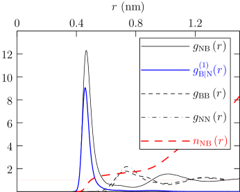
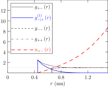
Figure 1: Upper-panel: Ion-ion radial distribution functions for atomically-detailed simulation Yang et al. (2009, 2010) of tetraethylammonium tetrafluoroborate in propylene carbonate ([tea][BF₄]/PC) at $T$ = 300 K, $p$ = 1 atm, and the slightly supersaturated concentration of 1 mol/dm³. $g_{\mathrm{B|N}}^{(1)}(r)$ is the radial distribution of the nearest B-neighbor of an N-atom. Lower panel: Results for a corresponding primitive model with dielectric constant and with ion charges and sizes matched to the [tea][BF₄]/PC case above. Specifically the model dielectric constant is $\epsilon=60$, and $d_{++}=0.6668$ nm, $d_{--}=0.6543$ nm, $d_{-+}=0.45$ nm are distances of closest approach for the hard spherical ions. The lower panel was produced by Monte Carlo simulation of a neutral system of 2$\times$500 hard spherical ions in conventional cubical periodic boundary conditions at the same temperature and concentration as the results above, utilizing the TowheeMartin (2010) package adapted to the present system.

As discussed below, the Poisson result Eq. (3) follows from a maximum entropy development when the information supplied is the expected occupancy of the inner-shell.Hummer et al. (1996); Pratt, Garde, and Hummer (1999); Pratt (2002) That information is sufficient if the occupancy $n\left(r\right)$ is always low, i.e., rarely larger than one. Thus, in contrast to the Fuoss approximation, Eq. (4) is correct for small $r$ because the expected coordination number tends to zero then. For the same reason, the Poisson approximation Eq. (3) is correct at low electrolyte concentration, and even when the solvent is treated at atomic resolution. Furthermore, it is natural to guess cation-anion chain or ring structures when ionic interactions drive well developed clustering. FIG. 1 shows a mean coordination number of less than two for counter-ion neighbors closer than about 0.5 nm, and supports the chain/ring picture of ion clusters formed. It is plausible therefore that a choice of inner-shell radii leading to small coordination numbers should validly describe important features of well-developed ion-clustering.

For computational analysis of reactive bi-molecular encounters in solution, identification of geometries of closest molecular pairs is critical.Chempath et al. (2008, 2010) Because it is correct for low concentration and for small $r$ in any case, Eq. (4) should be regarded as the general resolution of those questions.

When coordination numbers exceed one with reasonable probability, information on the expected number of pairs of counter-ions in the inner-shell should improve a maximum entropy model of these probabilities.Hummer et al. (1996); Pratt, Garde, and Hummer (1999); Pratt (2002) A maximum entropy model involving pair information would predict the $g_{\mathrm{\alpha|\gamma}}^{(1)}(r)\neq g_{\mathrm{\gamma|\alpha}}^{(1)}(r)$ asymmetry. For a 1-1 electrolyte, the generalization Eq. (4) is symmetrical in accord with the Fuoss approximation. The extent to which the observed asymmetry is significant gives an indication whether the Poisson approximation is adequate.

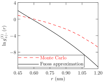
Figure 2: Comparison of the Fuoss approximation for $g_{\mathrm{+|-}}^{(1)}(r)$ to Monte Carlo results of FIG. 1.

Figure 3: An example showing that the distribution of anions nearest to a cation is generally different from the distribution of the cations nearest to an anion. The dashed lines indicate the nearest distances of a cation to each of the three anions. The solid lines mark the nearest distances of a anion to each of the three cations.

In this work, the Poisson approximation (Eq. (4)) is tested using three distinct simulation data sets. Two of these data sets have been noted already in considering FIG. 1. Those calculations treated solutions of tetraethylammonium tetrafluoroborate in propylene carbonate, one at atomic resolution ([tea][BF₄]/PC) and the other on the basis of a primitive electrolyte solution model over a range of concentrations. The third data set treated the ionic liquid 1-butyl-3-methylimidazolium tetrafluoroborate ([bmim][BF₄]). To ensure the correct correspondence of the necessary simulation details with the results as they are discussed, those details are provided in the captions of the figures providing the simulation results.

II Results and Discussion

For [tea][BF₄]/PC, comparison (FIG. 4) of the numerical data with the approximation Eq. (4) shows agreement over a distance range wider than the sizes of the molecules as judged by the radial distributions (FIG. 1). These near-neighbor distributions show bi-modal probability densities with maxima at $r\approx$ 0.5 nm and 0.9 nm. These correspond, respectively, to a contact ion pair and to a solvent-separated near-neighbor ion-pair. Thus the Poisson approximation Eq. (4) in this case includes solvation structure in characterizing inter-ionic neighborship.

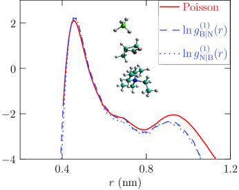
Figure 4: For the [tea][BF₄]/PC case of FIG. 1, comparison of the numerical data with the approximation Eq. (4). The local maximum at $r\approx$ 0.9 nm identifies solvent-separated nearest-neighbor ion-pairs. In this case, asymmetry of the two observed near-neighbor distributions is slight. That suggests that more elaborate maximum entropy models are unnecessary, and indeed the Poisson approximation is accurate. The embedded molecular graphic shows one of the solvent-separated nearest-neighbor BF${}_{4}{}^{-}$…PC …tea⁺ structures observed.

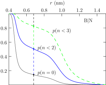
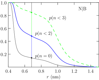
Figure 5: Occupancy probabilities as functions of the observation sphere radii $r$ for the [tea][BF₄]/PC case of FIG. 1. Upper panel: probabilities for occupancy by the B-atom of the BF${}_{4}{}^{-}$ anion of the inner-sphere of the N-atom of tetraethylammonium cation (tea⁺). Lower panel: probabilities for occupancy by the N-atom of the cation of the inner-sphere of the B-atom of the anion. The curves lowest in each panel are similar, showing symmetry displayed also in FIG. 4.

A plateau between $r\approx$ 0.5 nm and 0.9 nm in occupancy probabilities (FIG. 5) indicates saturation of counter-ion probability, and marks the inter-shell region. At the distance $r$ indicated by the vertical line, the coordination numbers $n$ = 1, 2 predominate, supporting the idea of the formation of cation-anion chain and ring structures. The two sets of probabilities (FIG. 5) are qualitatively similar, reinforcing the symmetry of FIG. 4.

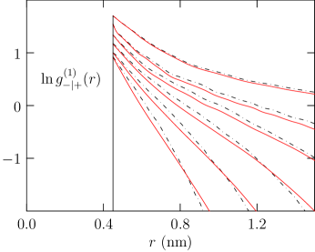
Figure 6: Dashed curves are Monte Carlo results for the primitive model of FIG. 1 and the solid lines are the Poisson approximation, Eq. (4). From top to bottom, the distinct cases correspond to concentrations 0.01, 0.05, 0.10, 0.20, 0.40, and 0.80 mol/dm³, $T$ = 300K for each case. For the highest concentration, the system size is 2$\times$400 ions. For all other cases, the system size is 2$\times$200 ions. At the lowest concentration here the distribution of the nearest neighbor $g_{-|+}^{(1)}(r)$ is close to the full radial distribution function $g_{+-}(r)$.

Results (FIG. 6) for the primitive model of FIG. 1 examine the sufficiency of the Poisson approximation over a broader concentration range for such models. The nearest-neighbor distributions are unimodal in this case. Correct at small $r$ where the probability densities are highest and properly normalized, the Poisson approximation Eq. (4) is accurate over the whole range shown.

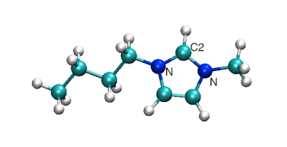
Figure 7: Structures and atom labeling of cation 1-butyl-3-methylimidazolium (bmim⁺) (top) and anion tetrafluoroborate (BF${}_{4}{}^{-}$). On the cation molecule, white, turquoise and dark blue balls stand for hydrogen, carbon, and nitrogen atoms, respectively. On the anion, white and green balls stand for fluorine and boron atoms, respectively.

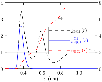
Figure 8: Radial distribution function of C2 atom on bmim⁺ cation and boron on BF${}_{4}{}^{-}$ anion obtained from MD simulation. Force field parameters and partial charge of the atoms were taken from Andrade et al.de Andrade, Böes, and Stassen (2002) The initial unit cell, with a dimension of 40 $\times$ 40 $\times$ 40 Å is uniformly packed with 190 ion pairs using Packmol.Martínez et al. (2009) MD simulation was performed using AMBER10 at constant pressure (1 bar) and temperature (298.5K). The system was first minimized, followed by 0.2ns equilibrium at a time step of 0.2 fs, then 1.3 ns equilibrium at a time step of 2 fs. Radial distribution functions were extracted from a production run of 3.0 ns.

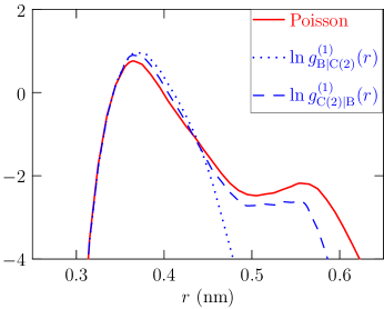
Figure 9: Nearest-neighbor distributions for the ionic liquid case of FIG. 8. In this case with no solvent, the asymmetry of the two observed near-neighbor distributions is marked. An outer-sphere nearest-neighbor is exhibited in one case but not the other case where the Poisson approximation Eq. (4) is inaccurate.

Another example is the ionic liquid [bmim][BF₄], with molecular structure shown in FIG. 7 and radial distribution functions in FIG. 8. The Poisson approximation (Eq. (4)) agrees with the observed $g_{\mathrm{C2|B}}^{(1)}(r)$ at short range and displays a second maximum characterizing non-contact nearest neighbors, though in this case there is no additional solvent. The near-neighbor B$|$C2 distribution (FIG. 9), on the other hand, lacks a second maximum. Thus $g_{\mathrm{C2|B}}^{(1)}(r)$ and $g_{\mathrm{B|C2}}^{(1)}(r)$ for ionic liquid [bmim][BF₄] display the generally expected asymmetry. This asymmetry is also reflected in occupancy probability profiles (FIG. 10). More general theoretical models are required for such cases, and we return to that theoretical discussion now.

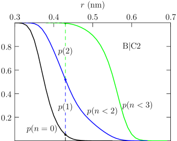
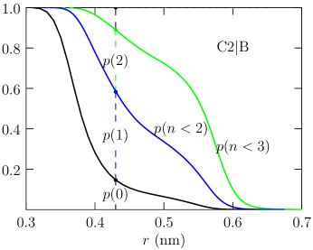
Figure 10: Occupancy probabilities as functions of the observation sphere radii $r$ for [bmim][BF₄] (FIG. 8). Upper panel: probabilities for occupancy by the B-atom of the BF${}_{4}{}^{-}$ anion of the inner-sphere of the mid-C-atom of 1-butyl-3-methylimidazolium (bmim⁺) cation (labeled as C2 in FIG. 7). Lower panel: probabilities for occupancy by the mid-C-atom of the cation of the inner-sphere of the B-atom of the anion. These results illustrate the possibility of a structural motif of ion clusters as chains and rings, i.e. at the $r$ = 0.43 nm distance of the vertical dashed line probabilities of 1 and 2 neighbors predominate. They also demonstrate asymmetry of the distributions of near-neighbor distances in their dependence on choice of the central ion, i.e. the distribution of nearest anions to a cation is different from the distribution of the nearest cations to an anion. Since $p(3)$ is larger in the lower panel than in the upper panel, the BF${}_{4}{}^{-}$ anion is more likely to be a three-way junction in this analysis than is the bmim⁺ cation.

III Maximum Entropy Modeling

The Poisson distribution $\hat{p}\left(n\right)=\left\langle n\right\rangle^{n}\mathrm{e}^{-\left\langle n\right\rangle}/{n!}$ describes random occupancy consistent with the information $\left\langle n\right\rangle=\left\langle n(r)\right\rangle$. Considering the relative entropy,

$$\eta(\{p\left(n\right)\})=~{}-\sum_{n\geq 0}p\left(n\right)\ln\left(\frac{p\left(n\right)}{\hat{p}\left(n\right)}\right)~{},$$ (5)

the Poisson distribution is a maximum entropy distribution satisfying the specific expected occupancy. If we have more information, e.g., the binomial momentsHummer et al. (1996); Pratt, Garde, and Hummer (1999); Pratt (2002)

$$\left\langle\binom{n}{j}\right\rangle=\sum_{n\geq 0}p\left(n\right)\left(\frac{n!}{(n-j)!j!}\right)~{},$$ (6)

we can seek the distribution which maximizes $\eta(\{p\left(n\right)\})$ and satisfies the broader set of information.

With the binomial moments (Eq. (6)), the Poisson distribution is seen to be correct if realized values of $n$ are rarely bigger than one (1). If $n$ is never 2 or larger, binomial moments $j\geq 2$ vanish. When $j\geq 2$ binomial moments are small, and that is consistent with Poisson prediction that they are zero. This underlies our observation above the the Poisson model, $p\left(0\right)\approx\mathrm{e}^{-\left\langle n\right\rangle}$ of Eq. (3), is correct for small $\lambda$.

Beyond the mean occupancy, the next level of information is the pair-correlation information $\left\langle n(r)\left(n(r)-1\right)/2\right\rangle$, the expected number of pairs of counter-ions in the indicated inner-shell. Carrying-out the maximization for the case that pair information is available induces the model $p(n)\propto\exp\left[-\lambda_{1}n-\lambda_{2}n(n-1)/2\right]/n!$, where $\lambda_{1}$, and $\lambda_{2}$ are Lagrange multipliers adjusted to reproduce the information $\left\langle n\right\rangle$ and $\left\langle n\left(n-1\right)/2\right\rangle$. Explicitly addressing the normalization of these probabilities leads to

$$p\left(n\right)=\frac{\left(\frac{1}{n!}\right)\mathrm{e}^{-\lambda_{1}n-\lambda_{2}n(n-1)/2}}{1+\sum\limits_{m\geq 1}\left(\frac{1}{m!}\right)\mathrm{e}^{-\lambda_{1}m-\lambda_{2}m(m-1)/2}}~{},$$ (7)

and

$$\ln p(0)=-\ln\left[1+\sum\limits_{n=1}^{\infty}\left(\frac{1}{n!}\right)\mathrm{e}^{-\lambda_{1}n-\lambda_{2}n(n-1)/2}\right]~{}.$$ (8)

$p(0)$ involves only the denominator of Eq. (7), and can be considered a partition function sum over occupancy states with $n$-dependent interactions and interaction strengths adjusted to satisfy the available information. The information required (FIG. 11) for this augmented maximum-entropy model is only subtly different for the two cases. Nevertheless, the results (FIG. 12) agree nicely with the observed asymmetry.

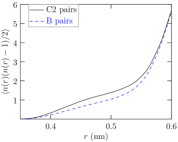
Figure 11: Pair information required for the augmented maximum entropy prediction of Eq. (8). Solid curve: the number of C2 pairs occupying a sphere of radius $r$ on a B atom. Dashed curve: the number of B pairs occupying a sphere of radius $r$ on a C2 atom.

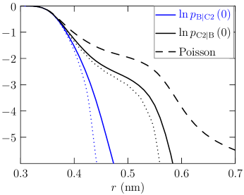
Figure 12: Analysis of the asymmetric $n=0$ probabilities of FIG. 10. Solid curves: direct numerical simulation as in FIG. 10; Dashed curve: Poisson-based approximation, Eq. (4); Dotted curves: augmented maximum entropy model utilizing the first two binomial moments, Eq. (8). The two-moment maximum entropy model is qualitatively reliable and therefore gives a satisfactory explanation of the observed asymmetry.

IV Conclusion

Results for both the [tea][BF₄]/PC (FIG. 1) and the ionic liquid [bmim][BF₄] (FIG. 8) identify a natural clustering radius where mean coordination numbers are near two. This suggests arrangements of the closest neighbors leading to a structural motif of cation-anion chains and rings. In contrast to the atomically detailed [tea][BF₄]/PC results, a corresponding primitive model (FIG. 1) does not display those clustering signatures (FIG. 6). A generalization (Eq. (4)) of the Fuoss ion-pairing model was obtained by recognizing that the Poisson distribution is correct when the mean coordination numbers are low. On the basis of measurable molecular distribution functions, this generalization also establishes the distribution of molecular nearest neighbors for computational analysis of bi-molecular reactive processes in solution. This Poisson-based model is accurate for the [tea][BF₄]/PC results, both for the primitive model and the atomically detailed case. For [tea][BF₄]/PC, the atomically detailed numerical results and the statistical model identify solvent-separated nearest-neighbor ion-pairs. Distributions of nearest-neighbor distances typically depend on which ion of a pair is taken as the central ion, i.e., the distribution of anions nearest to a cation is different from the distribution of the cations nearest to an anion. The Poisson-based model is not asymmetric in that way. The numerical data for the ionic liquid [bmim][BF₄] prominently show the expected asymmetry. That asymmetry can be treated by a maximum entropy model based on the expected number of pairs of counter-ions occupying the inner-shell of the central ion, information extracted from the simulations.

References

- Robinson and Stokes (2002) R. A. Robinson and R. H. Stokes, Electrolyte Solutions (Dover Publications Inc., Mineola, NY, 2002).
- Bjerrum (1926) N. Bjerrum, Kgl. Dan. Vidensk. Selsk. Mat-fys. Medd. 7, 1 (1926).
- Fuoss (1934) R. M. Fuoss, Trans. Faraday Soc. 30, 967 (1934).
- Fowler and Guggenheim (1949) R. Fowler and E. A. Guggenheim, Statistical Thermodynamics (Cambridge University Press, 1949) chapter IX.
- Reiss (1956) H. Reiss, J. Chem. Phys. 25, 400 (1956).
- Friedman (1961) H. L. Friedman, Ann. Rev. Phys. Chem. 12, 171 (1961).
- Stillinger Jr and Lovett (1968) F. H. Stillinger Jr and R. Lovett, J. Chem. Phys. 48, 1 (1968).
- Given and Stell (1997) J. Given and G. Stell, J. Chem. Phys. 106, 1195 (1997).
- Camp and Patey (1999a) P. Camp and G. N. Patey, J. Chem. Phys. 111, 9000 (1999a).
- Camp and Patey (1999b) P. J. Camp and G. N. Patey, Phys. Rev. E 60, 1063 (1999b).
- Kaneko (2005) T. Kaneko, J. Chem. Phys. 123, 134509 (2005).
- Yang et al. (2009) L. Yang, B. H. Fishbine, A. Migliori, and L. R. Pratt, J. Am. Chem. Soc. 131, 12373 (2009).
- Yang et al. (2010) L. Yang, B. H. Fishbine, A. Migliori, and L. R. Pratt, J. Chem. Phys. 132, 044701 (2010).
- Martin (2010) M. G. Martin, “Towhee,” Tech. Rep. (2010) http://sourceforge.net/projects/towhee/.
- Mazur (1992) S. Mazur, J. Chem. Phys. 97, 9276 (1992).
- Chandrasekhar (1943) S. Chandrasekhar, Rev. Mod. Phys. 15, 1 (1943).
- Hummer et al. (1996) G. Hummer, S. Garde, A. E. García, A. Pohorille, and L. R. Pratt, Proc. Natl. Acad. Sci USA 93, 8951 (1996).
- Pratt, Garde, and Hummer (1999) L. R. Pratt, S. Garde, and G. Hummer, NATO ADVANCED SCIENCE INSTITUTES SERIES, SERIES C, MATHEMATICAL AND PHYSICAL SCIENCES 529, 407 (1999).
- Pratt (2002) L. R. Pratt, Ann. Rev. Phys. Chem. 53, 409 (2002).
- Chempath et al. (2008) S. Chempath, B. R. Einsla, L. R. Pratt, C. S. B. J. M. Macomber, J. A. Rau, and B. S. Pivovar, J. Phys. Chem. C. 112, 3179 (2008).
- Chempath et al. (2010) S. Chempath, J. M. Boncella, L. R. Pratt, N. Henson, and B. S. Pivovar, J. Phys. Chem. C 114, 11977 (2010).
- de Andrade, Böes, and Stassen (2002) J. de Andrade, E. S. Böes, and H. Stassen, J. Phys. Chem. B 106, 13344 (2002).
- Martínez et al. (2009) L. Martínez, R. Andrade, E. G. Birgin, and J. M. Martínez, J. Comp. Chem. 30, 2157 (2009).