An Improved Algorithm for Reconstructing a Simple Polygon from the Visibility Angles

Abstract

In this paper, we study the following problem of reconstructing a simple polygon: Given a cyclically ordered vertex sequence of an unknown simple polygon $P$ of $n$ vertices and, for each vertex $v$ of $P$, the sequence of angles defined by all the visible vertices of $v$ in $P$, reconstruct the polygon $P$ (up to similarity). An $O(n^{3}\log n)$ time algorithm has been proposed for this problem. We present an improved algorithm with running time $O(n^{2})$, based on new observations on the geometric structures of the problem. Since the input size (i.e., the total number of input visibility angles) is $\Theta(n^{2})$ in the worst case, our algorithm is worst-case optimal.

1 Introduction

In this paper, we study the problem of reconstructing a simple polygon $P$ from the visibility angles measured at the vertices of $P$ and from the cyclically ordered vertices of $P$ along its boundary. Precisely, for an unknown simple polygon $P$ of $n$ vertices, suppose we are given (1) the vertices ordered counterclockwise (CCW) along the boundary of $P$, and (2) for each vertex $v$ of $P$, the angles between any two adjacent rays emanating from $v$ to the vertices of $P$ that are visible to $v$ such that these angles are in the CCW order as seen around $v$, beginning at the CCW neighboring vertex of $v$ on the boundary of $P$ (e.g., see Fig. 1). A vertex $u$ of $P$ is visible to a vertex $v$ of $P$ if the line segment connecting $u$ and $v$ lies entirely in $P$. The objective of the problem is to reconstruct the simple polygon $P$ (up to similarity) that fits all the given angles. We call this problem the polygon reconstruction problem from angles, or PRA for short. Figure 2 gives an example.

Figure 1: Illustrating the angle measurement at a vertex $v$: The angle sequence $(\alpha_{1},\alpha_{2},\alpha_{3},\alpha_{4})$ is given.

The PRA problem has been studied by Disser, Mihalák, and Widmayer [6], who showed that the solution polygon for the input is unique (up to similarity) and gave an $O(n^{3}\log n)$ time algorithm for reconstructing such a polygon. Using the input, their algorithm first constructs the visibility graph $G$ of $P$ and subsequently reconstructs the polygon $P$. As shown in [6], once $G$ is known, the polygon $P$ can be obtained efficiently (e.g., in $O(n^{2})$ time) with the help of the angle data and the CCW ordered vertex sequence of $P$.

Given a visibility graph $G$, the problem of determining whether there is a polygon $P$ that has $G$ as its visibility graph is called the visibility graph recognition problem, and the problem of actually constructing such a polygon $P$ is called the visibility graph reconstruction problem. Note that the general visibility graph recognition and reconstruction problems are long-standing open problems with only partial results known (e.g., see [1] for a short survey). Everett [8] showed that the visibility graph reconstruction problem is in PSPACE, but no better upper bound on the complexity of either problem is known. In our problem setting, we have the angle data information and the ordered vertex list of $P$; thus $P$ can be constructed efficiently after knowing $G$.

Hence, the major part of the algorithm in [6] is dedicated to constructing the visibility graph $G$ of $P$. As indicated in [6], the key difficulty is that the vertices in this problem setting have no recognizable labels, e.g., the angle measurement at a vertex $v$ gives angles between visible vertices to $v$ but does not identify these visible vertices globally. The authors in [6] also showed that some natural greedy approaches do not seem to work. An $O(n^{3}\log n)$ time algorithm for constructing $G$ is given in [6]. The algorithm, called the triangle witness algorithm, is based on the following observation: Suppose we wish to determine whether a vertex $v_{i}$ is visible to another vertex $v_{j}$; then $v_{i}$ is visible to $v_{j}$ if and only if there is a vertex $v_{l}$ on the portion of the boundary of $P$ from $v_{i+1}$ to $v_{j-1}$ in the CCW order such that $v_{l}$ is visible to both $v_{i}$ and $v_{j}$ and the triangle formed by the three vertices $v_{i},v_{j}$, and $v_{l}$ does not intersect the boundary of $P$ except at these three vertices (such a vertex $v_{l}$ is called a triangle witness vertex).

In this paper, based on the triangle witness algorithm [6], by exploiting some new geometric properties, we give an improved algorithm with a running time of $O(n^{2})$. The improvement is due to two key observations. First, in the triangle witness algorithm [6], to determine whether a vertex $v_{i}$ is visible to another vertex $v_{j}$, the algorithm needs to determine whether there exists a triangle witness vertex along the boundary of $P$ from $v_{i+1}$ to $v_{j-1}$ in the CCW order; to this end, the algorithm checks every vertex in that boundary portion of $P$. We observe that it suffices to check only one particular vertex in that boundary portion. This removes an $O(n)$ factor from the running time of the triangle witness algorithm [6]. Second, some basic operations in the triangle witness algorithm [6] take $O(\log n)$ time each; by utilizing certain different data structures, our new algorithm can handle each of those basic operations in constant time. This removes another $O(\log n)$ factor from the running time. Note that since the input size is $\Theta(n^{2})$ in the worst case (e.g., the total number of all visibility angles), our algorithm is worst-case optimal.

As shown in [6], if only the angle measurements are given, i.e., the ordered vertices along the boundary of $P$ are unknown, then the information is not sufficient for reconstructing $P$. In other words, it may be possible to compute several simple polygons that are not similar but all fit the given measured angles (see [6] for an example).

Figure 2: The given measured angles are ordered CCW along the polygon boundary (left); reconstructing a simple polygon that fits these angles (right).

1.1 Related Work

The problems of reconstructing geometric objects based on measurement data have been studied extensively (e.g., [2, 3, 12, 14, 15]). As discussed above, the general visibility graph recognition and reconstruction problems are in PSPACE [8] and no better complexity upper bound is known so far (e.g., see [10]). Yet, some results have been given for certain special polygons. For example, Everett and Corneil [9] characterized the visibility graphs of spiral polygons and gave a linear time reconstruction algorithm. Choi, Shin, and Chwa [4], and Colley, Lubiw, and Spinrad [5] characterized and recognized the visibility graphs of funnel-shaped polygons.

By adding extra information, some versions of the problems become more tractable. O’Rourke and Streinu [13] considered the vertex-edge visibility graph that includes edge-to-edge visibility information. Wismath [17] introduced the stab graphs which are also an extended visibility structure and showed how parallel line segments can be efficiently reconstructed from it. Snoeyink [15] proved that a unique simple polygon (up to similarity) can be determined by the interior angles at its vertices and the cross-ratios of the diagonals of any given triangulation, where the cross-ratio of a diagonal is the product of the ratios of edge lengths for the two adjacent triangles. Jackson and Wismath [12] studied the reconstruction of orthogonal polygons from horizontal and vertical visibility information and gave an $O(n\log n)$ time reconstruction algorithm. Biedl, Durocher, and Snoeyink [2] considered the problem of reconstructing the two-dimensional floor plan of a polygonal room using different types of scanned data, and proposed several problem models. Sidlesky, Barequet, and Gotsman [14] studied the problem of reconstructing a planar polygon from its intersections with a collection of arbitrarily-oriented “cutting” lines.

Reconstructing a simple polygon from angle data was first considered by Bilò et al. [3], who aimed to understand what kinds of sensorial capabilities are sufficient for a robot moving inside an unknown polygon to reconstruct the visibility graph of the polygon. It was shown in [3] that if the robot is equipped with a compass to measure the angle between any two vertices that are currently visible to the robot and also has the ability to know where it came from when moving from vertex to vertex, then the visibility graph of the polygon can be uniquely reconstructed. Reconstruction and exploration of environments by robots in other problem settings have also been studied (e.g., see [7, 11, 16]).

The rest of this paper is organized as follows. In Section 2, we give the problem definitions in detail and introduce some notations and basic observations. To be self-contained, in Section 3, we briefly review the triangle witness algorithm given in [6]. We then present our improved algorithm in Section 4.

2 Preliminaries

In this section, we define the PRA problem in detail and introduce the needed notations and terminology. For ease of discussion and comparison, some of our notations follow those in [6].

Let $P$ be a simple polygon of $n$ vertices $v_{0},v_{1},\ldots,v_{n-1}$ in the CCW order along $P$’s boundary. Denote by $G=(V,E)$ the visibility graph of $P$, where $V$ consists of all vertices of $P$ and for any two distinct vertices $v_{i}$ and $v_{j}$, $E$ contains an edge $e(v_{i},v_{j})$ connecting $v_{i}$ and $v_{j}$ if and only if $v_{i}$ is visible to $v_{j}$ inside $P$. In this paper, the indices of all $v_{i}$’s are taken as congruent modulo $n$, i.e., if $n\leq i+j\leq 2n-1$, then $v_{i+j}$ is the same vertex as $v_{l}$, where $l=i+j-n$ (or $l=(i+j)\mod n$); similarly, if $-n\leq i-j<0$, then $v_{i-j}$ is the same vertex as $v_{l}$, where $l=i-j+n$. For each $v_{i}\in V$, denote by $deg(v_{i})$ its degree in the visibility graph $G$, and denote by $vis(v_{i})=(vis_{1}(v_{i}),vis_{2}(v_{i}),\ldots,vis_{deg(v_{i})}(v_{i}))$ the sequence of vertices in $P$ visible to $v_{i}$ from $v_{i+1}$ to $v_{i-1}$ ordered CCW around $v_{i}$. We refer to $vis(v_{i})$ as $v_{i}$’s visibility angle sequence. Note that since both $v_{i-1}$ and $v_{i+1}$ are visible to $v_{i}$, $vis_{1}(v_{i})=v_{i+1}$ and $vis_{deg(v_{i})}(v_{i})=v_{i-1}$. For any two vertices $v_{i},v_{j}$ in $V$, let $ch(v_{i},v_{j})$ denote the sequence $(v_{i},v_{i+1},\ldots,v_{j})$ of the vertices ordered CCW along the boundary of $P$ from $v_{i}$ to $v_{j}$. We refer to $ch(v_{i},v_{j})$ as a chain. Let $|ch(v_{i},v_{j})|$ denote the number of vertices of $P$ in the chain $ch(v_{i},v_{j})$.

For any two distinct vertices $v_{i},v_{j}\in P$, let $\rho(v_{i},v_{j})$ be the ray emanating from $v_{i}$ and going towards $v_{j}$. For any three vertices $v,v_{i},v_{j}\in P$, denote by $\angle_{v}(v_{i},v_{j})$ the CCW angle defined by rotating $\rho(v,v_{i})$ around $v$ to $\rho(v,v_{j})$ ($v_{i}$ or $v_{j}$ need not be visible to $v$). Note that the values of all angles we use in this paper are in $[0,2\pi)$. For any vertex $v\in P$ and $1\leq i<j\leq deg(v)$, let $\angle_{v}(i,j)$ be $\angle_{v}(vis_{i}(v),vis_{j}(v))$.

The PRA problem can then be re-stated as follows: Given a sequence of all vertices $v_{0},v_{1},\ldots,v_{n-1}$ of an unknown simple polygon $P$ in the CCW order along $P$’s boundary, and the angles $\angle_{v}(i,i+1)$ for each vertex $v$ of $P$ with $1\leq i<deg(v)$, we seek to reconstruct $P$ (up to similarity) to fit all the given angles. Without loss of generality, we assume that no three distinct vertices of $P$ are collinear.

It is easy to see that after $O(n^{2})$ time preprocessing, for any $v\in V$ and any $1\leq i<j\leq deg(v)$, the angle $\angle_{v}(i,j)$ can be obtained in constant time. In the following discussion, we assume that this preprocessing has already been done. Sometimes we (loosely) say that these angles are given as input.

The algorithm given in [6] does not construct $P$ directly. Instead, the algorithm first computes its visibility graph $G=(V,E)$. As mentioned earlier, after knowing $G$, $P$ can be reconstructed efficiently with the help of the angle data and the CCW ordered vertex sequence of $P$. The algorithm for constructing $G$ in [6] is called the triangle witness algorithm, which will be briefly reviewed in Section 3. Since $V$ consists of all vertices of $P$, the problem of constructing $G$ is equivalent to constructing its edge set $E$, i.e., for any two distinct vertices $v_{i},v_{j}\in P$, determine whether there is an edge $e(v_{i},v_{j})$ in $E$ connecting $v_{i}$ and $v_{j}$ (in other words, determining whether $v_{i}$ is visible to $v_{j}$ inside $P$).

To discuss the involved algorithms, we need one more definition. For any two vertices $v_{i},v_{j}\in P$ with $|ch(v_{i+1},v_{j-1})|\geq 1$, suppose a vertex $v_{l}\in ch(v_{i+1},v_{j-1})$ is visible to both $v_{i}$ and $v_{j}$; then we let $v_{j}^{\prime}$ be the first visible vertex to $v_{i}$ on the chain $ch(v_{j},v_{i})$ and let $v_{i}^{\prime}$ be the last visible vertex to $v_{j}$ on the chain $ch(v_{j},v_{i})$ (e.g., see Fig. 3). Intuitively, imagine that we rotate a ray from $\rho(v_{i},v_{l})$ around $v_{i}$ counterclockwise; then the first vertex on the chain $ch(v_{j},v_{i})$ hit by the rotating ray is $v_{j}^{\prime}$. Similarly, if we rotate a ray from $\rho(v_{j},v_{l})$ around $v_{j}$ clockwise, then the first vertex on the chain $ch(v_{j},v_{i})$ hit by the rotating ray is $v_{i}^{\prime}$. Note that if $v_{i}$ is visible to $v_{j}$, then $v_{j}^{\prime}$ is $v_{j}$ and $v_{i}^{\prime}$ is $v_{i}$. We denote by $\angle^{\uparrow}_{v_{i}}(v_{l},v_{j})$ the angle $\angle_{v_{i}}(v_{l},v_{j}^{\prime})$ and denote by $\angle^{\uparrow}_{v_{j}}(v_{i},v_{l})$ the angle $\angle_{v_{j}}(v_{i}^{\prime},v_{l})$. It should be pointed out that for ease of understanding this paper, the above statement of defining $\angle^{\uparrow}$ is different from that in [6] but they refer to the same angles in the algorithm. The motivation for defining $\angle^{\uparrow}$ will be clear after discussing the following lemma, which has been proved in [6].

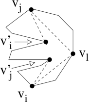
Figure 3: Illustrating the definitions of $v^{\prime}_{i}$ and $v_{j}^{\prime}$, and $\angle^{\uparrow}_{v_{i}}(v_{l},v_{j})$ and $\angle^{\uparrow}_{v_{j}}(v_{i},v_{l})$ which are the angles $\angle_{v_{i}}(v_{l},v_{j}^{\prime})$ and $\angle_{v_{j}}(v_{i}^{\prime},v_{l})$, respectively.

Lemma 1

[6] For any two vertices $v_{i},v_{j}\in P$ with $|ch(v_{i+1},v_{j-1})|\geq 1$, $v_{i}$ is visible to $v_{j}$ if and only if there exists a vertex $v_{l}$ on $ch(v_{i+1},v_{j-1})$ such that $v_{l}$ is visible to both $v_{i}$ and $v_{j}$ and $\angle^{\uparrow}_{v_{i}}(v_{l},v_{j})+\angle^{\uparrow}_{v_{j}}(v_{i},v_{l})+\angle_{v_{l}}(v_{j},v_{i})=\pi$.

Since the above lemma is also critical to our improved algorithm in Section 4, we sketch the proof of the lemma below.

For any two vertices $v_{i},v_{j}\in P$ with $|ch(v_{i+1},v_{j-1})|\geq 1$, if $v_{i}$ is visible to $v_{j}$, then it is not difficult to see that there must exist a vertex $v_{l}\in ch(v_{i+1},v_{j-1})$ that is visible to both $v_{i}$ and $v_{j}$. Since the three vertices $v_{i},v_{j}$, and $v_{l}$ are mutually visible to each other, it is clear that the triangle formed by these three vertices does not intersect the boundary of $P$ except at the three vertices, implying that $\angle^{\uparrow}_{v_{i}}(v_{l},v_{j})+\angle^{\uparrow}_{v_{j}}(v_{i},v_{l})+\angle_{v_{l}}(v_{j},v_{i})=\angle_{v_{i}}(v_{l},v_{j})+\angle_{v_{j}}(v_{i},v_{l})+\angle_{v_{l}}(v_{j},v_{i})=\pi$. Such a vertex $v_{l}$ is called a triangle witness of the edge $e(v_{i},v_{j})$ in $E$.

Suppose $v_{i}$ is not visible to $v_{j}$; then it is possible that there does not exist a vertex $v_{l}\in ch(v_{i+1},v_{j-1})$ which is visible to both $v_{i}$ and $v_{j}$. In fact, if there exists no vertex $v_{l}\in ch(v_{i+1},v_{j-1})$ that is visible to both $v_{i}$ and $v_{j}$, then $v_{i}$ cannot be visible to $v_{j}$. Hence in the following, we assume that such a vertex $v_{l}$ exists, i.e., a vertex $v_{l}\in ch(v_{i+1},v_{j-1})$ is visible to both $v_{i}$ and $v_{j}$ (yet $v_{i}$ is not visible to $v_{j}$). Note that $v_{l}$ is not collinear with $v_{i}$ and $v_{j}$. If $\angle_{v_{l}}(v_{j},v_{i})>\pi$ (i.e., the chain $ch(v_{i},v_{j})$ is part of the boundary of $P$ that blocks the visibility between $v_{i}$ and $v_{j}$), then the lemma obviously holds. Otherwise, $\angle_{v_{l}}(v_{j},v_{i})<\pi$, and in this case, the visibility between $v_{i}$ and $v_{j}$ is blocked by the chain $ch(v_{j},v_{i})$. Since $v_{i}$ is not visible to $v_{j}$, for any choice of such a vertex $v_{l}$, the angle $\angle_{v_{i}}(v_{l},v_{j})$ is not given by $v_{i}$’s visibility angle sequence $vis(v_{i})$. The “closest approximation” for $\angle_{v_{i}}(v_{l},v_{j})$ in this case is determined by a vertex $v$ on the chain $ch(v_{j},v_{i})$ such that $v$ becomes $v_{j}$ if and only if $v_{j}$ is visible to $v_{i}$. As in the definition of $\angle^{\uparrow}_{v_{i}}(v_{l},v_{j})$, the vertex $v_{j}^{\prime}$ is such a vertex $v$, i.e., the first visible vertex to $v_{i}$ on the chain $ch(v_{j},v_{i})$. Similarly, the vertex $v_{i}$ in $\angle_{v_{j}}(v_{i},v_{l})$ is “replaced” in the definition of $\angle^{\uparrow}_{v_{j}}(v_{i},v_{l})$ by $v_{i}^{\prime}$, i.e., the last visible vertex to $v_{j}$ on $ch(v_{j},v_{i})$. Clearly, when $v_{j}$ is not visible to $v_{i}$, it must hold that $\angle_{v_{i}}(v_{l},v_{j}^{\prime})<\angle_{v_{i}}(v_{l},v_{j})$ and $\angle_{v_{j}}(v_{i}^{\prime},v_{l})<\angle_{v_{j}}(v_{i},v_{l})$. Therefore, $\angle^{\uparrow}_{v_{i}}(v_{l},v_{j})+\angle^{\uparrow}_{v_{j}}(v_{i},v_{l})+\angle_{v_{l}}(v_{j},v_{i})=\angle_{v_{i}}(v_{l},v_{j}^{\prime})+\angle_{v_{j}}(v_{i}^{\prime},v_{l})+\angle_{v_{l}}(v_{j},v_{i})<\angle_{v_{i}}(v_{l},v_{j})+\angle_{v_{j}}(v_{i},v_{l})+\angle_{v_{l}}(v_{j},v_{i})=\pi$. Lemma 1 thus follows.

3 The Triangle Witness Algorithm

In this section, we briefly review the triangle witness algorithm in [6] that constructs the visibility graph $G=(V,E)$ of the unknown simple polygon $P$.

The triangle witness algorithm is based on Lemma 1. The algorithm has $\lceil n/2\rceil$ iterations. In the $k$-th iteration ($1\leq k\leq\lceil n/2\rceil$), the algorithm checks, for each $i=0,1,\ldots,n-1$, whether $v_{i}$ is visible to $v_{i+k}$. After all iterations, the edge set $E$ can be obtained. To this end, the algorithm maintains two maps $F$ and $B$: $F[v_{i}][v_{j}]=t$ if $v_{j}$ is identified as the $t$-th visible vertex to $v_{i}$ in the CCW order, i.e., $v_{j}=vis_{t}(v_{i})$; the definition of $B$ is the same as $F$. During the algorithm, $F$ will be filled in the CCW order and $B$ will be filled in the clockwise (CW) order. When the algorithm finishes, for each $v_{i}$, $F[v_{i}]$ will have all visible vertices to $v_{i}$ on the chain $ch(v_{i+1},v_{\lceil n/2\rceil})$ while $B[v_{i}]$ will have all visible vertices to $v_{i}$ on the chain $ch(v_{\lceil n/2\rceil},v_{i-1})$. Thus, $F[v_{i}]$ and $B[v_{i}]$ together contain all visible vertices of $P$ to $v_{i}$. For ease of description, we also treat $F[v_{i}]$ and $B[v_{i}]$ as sets, e.g., $v_{l}\in F[v_{i}]$ means that there is an entry $F[v_{i}][v_{l}]$ and $|F[v_{i}]|$ means the number of entries in the current $F[v_{i}]$.

Initially, when $k=1$, since every vertex is visible to its two neighbors along the boundary of $P$, we have $F[v_{i}][v_{i+1}]=1$ and $B[v_{i}][v_{i-1}]=deg(v_{i})$ for each $v_{i}$. In the $k$-th iteration, we determine for each $v_{i}$, whether $v_{i}$ is visible to $v_{i+k}$. Below, we let $j=i+k$. Note that $|F[v_{i}]|+1$ is the index of the first visible vertex to $v_{i}$ in the CCW order that is not yet identified; similarly, $(deg(v_{j})-|B[v_{j}]|)$ is the index of the first visible vertex to $v_{j}$ in the CW order that is not yet identified. If $v_{i}$ is visible to $v_{j}$, then we know that $v_{j}$ is the $(|F[v_{i}]|+1)$-th visible vertex to $v_{i}$ and $v_{i}$ is the $(deg(v_{j})-|B[v_{j}]|)$-th visible vertex to $v_{j}$, and thus we set $F[v_{i}][v_{j}]=|F[v_{i}]|+1$ and $B[v_{j}][v_{i}]=deg(v_{j})-|B[v_{j}]|$. If $v_{i}$ is not visible to $v_{j}$, then we do nothing.

It remains to discuss how to determine whether $v_{i}$ is visible to $v_{j}$. According to Lemma 1, we need to determine whether there exists a triangle witness vertex $v_{l}$ in the chain $ch(v_{i+1},v_{j-1})$, i.e., $v_{l}$ is visible to both $v_{i}$ and $v_{j}$ and $\angle^{\uparrow}_{v_{i}}(v_{l},v_{j})+\angle^{\uparrow}_{v_{j}}(v_{i},v_{l})+\angle_{v_{l}}(v_{j},v_{i})=\pi$. To this end, the algorithm checks every vertex $v_{l}$ in $ch(v_{i+1},v_{j-1})$. For each $v_{l}$, the algorithm first determines whether $v_{l}$ is visible to both $v_{i}$ and $v_{j}$, by checking whether there is an entry for $v_{l}$ in $F[v_{i}]$ and in $B[v_{j}]$. The algorithm utilizes balanced binary search trees to represent $F$ and $B$, and thus checking whether there is an entry for $v_{l}$ in $F[v_{i}]$ and in $B[j]$ can be done in $O(\log n)$ time. If $v_{l}$ is visible to both $v_{i}$ and $v_{j}$, then the next step is to determine whether $\angle^{\uparrow}_{v_{i}}(v_{l},v_{j})+\angle^{\uparrow}_{v_{j}}(v_{i},v_{l})+\angle_{v_{l}}(v_{j},v_{i})=\pi$. It is easy to know that $\angle_{v_{l}}(v_{j},v_{i})$ is $\angle_{v_{l}}(F[v_{l}][v_{j}],B[v_{l}][v_{i}])$, which can be found readily from the input. To obtain $\angle^{\uparrow}_{v_{i}}(v_{l},v_{j})$, we claim that it is the angle $\angle_{v_{i}}(F[v_{i}][v_{l}],|F[v_{i}]|+1)$. Indeed, observe that all visible vertices in the chain $ch(v_{i+1},v_{j-1})$ are in the current $F[v_{i}]$. As explained above, $|F[v_{i}]|+1$ is the index of the first visible vertex to $v_{i}$ in the CCW order that has not yet been identified, which is the first visible vertex to $v_{i}$ in the chain $ch(v_{j},v_{i})$, i.e, the vertex $v_{j}^{\prime}$. Thus, $\angle_{v_{i}}(F[v_{i}][v_{l}],|F[v_{i}]|+1)$ is $\angle_{v_{i}}(v_{l},v_{j}^{\prime})$, which is $\angle^{\uparrow}_{v_{i}}(v_{l},v_{j})$. Similarly, $\angle^{\uparrow}_{v_{j}}(v_{i},v_{l})$ is the angle $\angle_{v_{j}}(deg(v_{j})-|B[v_{j}]|,B[v_{j}][v_{l}])$. Note that both the angles $\angle_{v_{i}}(F[v_{i}][v_{l}],|F[v_{i}]|+1)$ and $\angle_{v_{j}}(deg(v_{j})-|B[v_{j}]|,B[v_{j}][v_{l}])$ are known. Algorithm 2 in the Appendix summarizes the whole algorithm [6].

To analyze the running time of the above triangle witness algorithm, note that it has $\lceil n/2\rceil$ iterations. In each iteration, the algorithm checks whether $v_{i}$ is visible to $v_{i+k}$ for each $0\leq i\leq n-1$. For each $v_{i}$, the algorithm checks every $v_{l}$ for $i+1\leq l\leq i+k-1$, i.e, in the chain $ch(v_{i+1},v_{i+k-1})$. For each such $v_{l}$, the algorithm takes $O(\log n)$ time as it uses balanced binary search trees to represent the two maps $F$ and $B$. In summary, the overall running time of the triangle witness algorithm in [6] is $O(n^{3}\log n)$.

4 An Improved Triangle Witness Algorithm

In this section, we present an improved solution over the triangle witness algorithm in [6] sketched in Section 3. Our improved algorithm runs in $O(n^{2})$ time. Since the input size (e.g., the total number of visibility angles) is $\Theta(n^{2})$ in the worst case, our improved algorithm is worst-case optimal. Our new algorithm follows the high-level scheme of the triangle witness algorithm in [6], and thus we call it the improved triangle witness algorithm.

As in [6], the new algorithm also has $\lceil n/2\rceil$ iterations, and in each iteration, we determine whether $v_{i}$ is visible to $v_{i+k}$ for each $0\leq i\leq n-1$. For every pair of vertices $v_{i}$ and $v_{i+k}$, let $j=i+k$. To determine whether $v_{i}$ is visible to $v_{j}$, the triangle witness algorithm [6] checks each vertex $v_{l}$ in the chain $ch(v_{i+1},v_{j-1})$ to see whether there exists a triangle witness vertex. In our new algorithm, instead, we claim that we need to check only one particular vertex, $vis_{|F[v_{i}]|}(v_{i})$, i.e., the last visible vertex to $v_{i}$ in the chain $ch(v_{i+1},v_{j-1})$ in the CCW order, as stated in the following lemma.

Figure 4: Illustrating Lemma 2: $v^{\prime}$ is $vis_{|F[v_{i}]|}(v_{i})$, the last visible vertex to $v_{i}$ in $ch(v_{i+1},v_{j-1})$; $v_{i}$ is visible to $v_{j}$ if and only if $v^{\prime}$ is a triangle witness vertex.

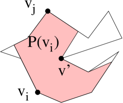
Figure 5: Illustrating the visibility polygon $P(i)$ for the example in Fig. 4: The gray (pink) area is $P(i)$, which is a star-shaped polygon with the vertex $v_{i}$ as a kernel point.

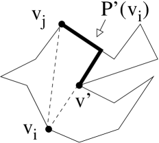
Figure 6: Illustrating $P^{\prime}(i)$ for the example in Fig. 4: The thick line segments form $P^{\prime}(i)$.

Lemma 2

The vertex $v_{i}$ is visible to $v_{j}$ if and only if the vertex $vis_{|F[v_{i}]|}(v_{i})$ is a triangle witness vertex for $v_{i}$ and $v_{j}$.

Proof: Let $v^{\prime}$ denote the vertex $vis_{|F[v_{i}]|}(v_{i})$, which is the last visible vertex to $v_{i}$ in the chain $ch(v_{i+1},v_{j-1})$ in the CCW order. Recall that $v^{\prime}$ being a triangle witness vertex for $v_{i}$ and $v_{j}$ is equivalent to saying that $v^{\prime}$ is visible to both $v_{i}$ and $v_{j}$ and $\angle^{\uparrow}_{v_{i}}(v^{\prime},v_{j})+\angle^{\uparrow}_{v_{j}}(v_{i},v^{\prime})+\angle_{v^{\prime}}(v_{j},v_{i})=\pi$.

If $v_{i}$ is visible to $v_{j}$, then we prove below that $v^{\prime}$ is a triangle witness vertex for $v_{i}$ and $v_{j}$, i.e., we prove that $v^{\prime}$ is visible to both $v_{i}$ and $v_{j}$ and $\angle^{\uparrow}_{v_{i}}(v^{\prime},v_{j})+\angle^{\uparrow}_{v_{j}}(v_{i},v^{\prime})+\angle_{v^{\prime}}(v_{j},v_{i})=\pi$. Refer to Fig. 4 for an example. Let $P(v_{i})$ denote the subpolygon of $P$ that is visible to the vertex $v_{i}$. Usually, $P(v_{i})$ is called the visibility polygon of $v_{i}$ and it is well-known that $P(v_{i})$ is a star-shaped polygon with $v_{i}$ as a kernel point (e.g., see [1]). Figure 5 illustrates $P(v_{i})$. Since $v^{\prime}$ is the last visible vertex to $v_{i}$ in $ch(v_{i+1},v_{j-1})$ and $v_{j}$ is visible to $v_{i}$, we claim that $v_{j}$ is also visible to $v^{\prime}$. Indeed, since both $v^{\prime}$ and $v_{j}$ are visible to $v_{i}$, $v^{\prime}$ and $v_{j}$ are both on the boundary of the visibility polygon $P(v_{i})$. Let $P^{\prime}(v_{i})$ denote the portion of the boundary of $P(v_{i})$ from $v^{\prime}$ to $v_{j}$ counterclockwise (see Fig. 6). We prove below that $P^{\prime}(v_{i})$ does not contain any vertex of $P$ except $v^{\prime}$ and $v_{j}$. First, $P^{\prime}(v_{i})$ cannot contain any vertex in the chain $ch(v_{j+1},v_{i-1})$ (otherwise, $v_{j}$ would not be visible to $v_{i}$). Let the index of the vertex $v^{\prime}$ be $l$, i.e., $v^{\prime}=v_{l}$. Similarly, $P^{\prime}(v_{i})$ cannot contain any vertex in the chain $ch(v_{i+1},v_{l-1})$ (otherwise, $v^{\prime}$ would not be visible to $v_{i}$). Finally, $P^{\prime}(v_{i})$ cannot contain any vertex in the chain $ch(v_{l+1},v_{j-1})$, since otherwise $v^{\prime}$ would not be the last visible vertex to $v_{i}$ in $ch(v_{i+1},v_{j-1})$. Thus, $P^{\prime}(v_{i})$ does not contain any vertex of $P$ except $v^{\prime}$ and $v_{j}$. Therefore, the region bounded by $P^{\prime}(v_{i})$, the line segment connecting $v_{i}$ and $v_{j}$, and the line segment connecting $v_{i}$ and $v^{\prime}$ must be convex (in fact, it is always a triangle) and this region is entirely contained in $P$. This implies that $v_{j}$ is visible to $v^{\prime}$. Hence, the three vertices $v_{i},v_{j}$, and $v^{\prime}$ are mutually visible to each other, and we have $\angle^{\uparrow}_{v_{i}}(v_{l},v_{j})+\angle^{\uparrow}_{v_{j}}(v_{i},v_{l})+\angle_{v_{l}}(v_{j},v_{i})=\angle_{v_{i}}(v_{l},v_{j})+\angle_{v_{j}}(v_{i},v_{l})+\angle_{v_{l}}(v_{j},v_{i})=\pi$.

On the other hand, if $v^{\prime}$ is a triangle witness vertex for $v_{i}$ and $v_{j}$, then by Lemma 1, the vertex $v_{i}$ is visible to $v_{j}$. The lemma thus follows. $\Box$

By Lemma 2, to determine whether $v_{i}$ is visible to $v_{j}$, instead of checking every vertex in $ch(v_{i+1},v_{j-1})$, we need to consider only the vertex $vis_{|F[v_{i}]|}(v_{i})$ in the current set $F[v_{i}]$. Hence, Lemma 2 immediately reduces the running time of the triangle witness algorithm by an $O(n)$ factor. The other $O(\log n)$ factor improvement is due to a new way of defining and representing the maps $F$ and $B$, as elaborated below. In the following discussion. let $v^{\prime}$ be the vertex $vis_{|F[v_{i}]|}(v_{i})$.

In our new algorithm, to determine whether $v_{i}$ is visible to $v_{j}$, we check whether $v^{\prime}$ is a triangle witness vertex for $v_{i}$ and $v_{j}$. To this end, we already know that $v^{\prime}$ is visible to $v_{i}$, but we still need to check whether $v^{\prime}$ is visible to $v_{j}$. In the previous triangle witness algorithm [6], this step is performed in $O(\log n)$ time by representing $F$ and $B$ using balanced binary search trees. In our new algorithm, we handle this step in $O(1)$ time, by redefining $F$ and $B$ and using a new way to represent them.

We redefine $F$ as follows: $F[v_{i}][v_{j}]=t$ if $v_{j}$ is the $t$-th visible vertex to $v_{i}$ in the CCW order; if $v_{j}$ is not visible to $v_{i}$ or $v_{j}$ has not yet been identified, then $F[v_{i}][v_{j}]=0$. For convenience, we let $F[v_{i}]=F[v_{i}][v_{i+1},v_{i+2},\ldots,v_{i-1}]$. Thus, in our new definition, the size of $F[v_{i}]$ is fixed throughout the algorithm, i.e., $|F[v_{i}]|$ is always $n-1$. In addition, for each $v_{i}$, the new algorithm maintains two variables $L_{i}$ and $I_{i}$ for $F[v_{i}]$, where $L_{i}$ is the number of non-zero entries in the current $F[v_{i}]$, which is also the number of visible vertices to $v_{i}$ that have been identified (i.e., the number of visible vertices to $v_{i}$ in the chain $ch(v_{i+1},v_{i+k-1})$) up to the $k$-th iteration, and $I_{i}$ is the index of the last non-zero entry in the current $F[v_{i}]$, i.e., $I_{i}$ is the last visible vertex to $v_{i}$ in the chain $ch(v_{i+1},v_{i+k-1})$ in the CCW order. Similarly, we redefine $B$ in the same way as $F$, i.e., for each $v_{i}$, $B[v_{i}]=B[v_{i}][v_{i+1},v_{i+2},\ldots,v_{i-1}]$ and $B[v_{i}][v_{j}]=t$ if $v_{j}$ is the $t$-th visible vertex to $v_{i}$ in the CCW order. Further, for each $v_{i}$, we also maintain two variables $L_{i}^{\prime}$ and $I_{i}^{\prime}$ for $B[v_{i}]$, where $L_{i}^{\prime}$ is the number of non-zero entries in the current $B[v_{i}]$, which is also the number of visible vertices to $v_{i}$ in the chain $ch(v_{i-k+1},v_{i-1})$ (up to the $k$-th iteration), and $I_{i}^{\prime}$ is the index of the first non-zero entry in the current $B[v_{i}]$, i.e., $I_{i}^{\prime}$ is the first visible vertex to $v_{i}$ in the chain $ch(v_{i-k+1},v_{i-1})$ in the CCW order. During the algorithm, the array $F[v_{i}]$ will be filled in the CCW order, i.e., from the first entry $F[v_{i}][v_{i+1}]$ to the end while the array $B[v_{i}]$ will be filled in the CW order, i.e, from the last entry $B[v_{i}][v_{i-1}]$ to the beginning. When the algorithm finishes, $F[v_{i}]$ will contain all the visible vertices to $v_{i}$ in the chain $ch(v_{i+1},v_{i+\lceil n/2\rceil})$, and thus only the entries of the first half of $F[v_{i}]$ are possibly filled with non-zero values. Similarly, only the entries of the second half of $B[v_{i}]$ are possibly filled with non-zero values. Below, we discuss the implementation details of our new algorithm, which is summarized in Algorithm 1.

Input: $n$, $(v_{1},v_{2},\ldots,v_{n})$, $deg(v_{i})$, and the angles $\angle_{v_{i}}(\cdot,\cdot)$ for each $0\leq i\leq n-1$.

Output: The edge set $E$ of the visibility graph $G$ for the target polygon $P$.

/* All indices below are understood modulo $n$. */

$E\leftarrow\emptyset$;

for $i\leftarrow 0$ to $n-1$ do

       $F[v_{i}][v_{i+1},v_{i+2},\ldots,v_{i-1}]\leftarrow 0$;

       $B[v_{i}][v_{i+1},v_{i+2},\ldots,v_{i-1}]\leftarrow 0$;

      

for $i\leftarrow 0$ to $n-1$ do

       $E\leftarrow E\cup\{e(v_{i},v_{i+1})\}$;

       $F[v_{i}][v_{i+1}]\leftarrow 1$;

       $B[v_{i}][v_{i-1}]\leftarrow deg(v_{i})$;

       $L_{i}\leftarrow 1,I_{i}\leftarrow v_{i+1},L^{\prime}_{i}\leftarrow 1,I_{i}^{\prime}\leftarrow v_{i-1}$;

      

for $k\leftarrow 2$ to $\lceil n/2\rceil$ do

       for $i\leftarrow 0$ to $n-1$ do

             $j\leftarrow i+k$;

             $v^{\prime}\leftarrow I_{i}$;

             if $B[v_{j}][v^{\prime}]>0$ then

                   $\angle^{\uparrow}_{v_{i}}(v^{\prime},v_{j})\leftarrow\angle_{v_{i}}(F[v_{i}][v^{\prime}],L_{i}+1)$;

                   $\angle^{\uparrow}_{v_{j}}(v_{i},v^{\prime})\leftarrow\angle_{v_{j}}(deg(v_{j})-L_{i}^{\prime},B[v_{j}][v^{\prime}])$;

                   $\angle_{v^{\prime}}(v_{j},v_{i})\leftarrow\angle_{v^{\prime}}(F[v^{\prime}][v_{j}],B[v^{\prime}][v_{i}])$;

                  

             if $\angle^{\uparrow}_{v_{i}}(v^{\prime},v_{j})+\angle^{\uparrow}_{v_{j}}(v_{i},v^{\prime})+\angle_{v^{\prime}}(v_{j},v_{i})=\pi$ then

                   $E\leftarrow E\cup\{e(v_{i},v_{j})\}$;

                   $F[v_{i}][v_{j}]\leftarrow L_{i}+1$;

                   $B[v_{j}][v_{i}]\leftarrow deg(v_{j})-L_{j}^{\prime}$;

                   $L_{i}\leftarrow L_{i}+1$, $L^{\prime}_{j}\leftarrow L^{\prime}_{j}+1$, $I_{i}\leftarrow v_{j}$, $I^{\prime}_{j}\leftarrow v_{i}$;

                  

            

      

Algorithm 1 The Improved Triangle Witness Algorithm

Initially, when $k=1$, for each $v_{i}$, we set $F[v_{i}][v_{i+1}]=1$ and $B[v_{i}][v_{i-1}]=deg(v_{i})$, and set all other entries of $F[v_{i}]$ and $B[v_{i}]$ to zero. In addition, we set $L_{i}=1$, $I_{i}=v_{i+1}$ and $L^{\prime}_{i}=1$, $I^{\prime}_{i}=v_{i-1}$. In the $k$-th iteration, with $1<k\leq\lceil n/2\rceil$, for each $v_{i}$, we check whether $v_{i}$ is visible to $v_{j}$, with $j=i+k$. If $v_{i}$ is not visible to $v_{j}$, then we do nothing. Otherwise, we set $F[v_{i}][v_{j}]=L_{i}+1$ and increase $L_{i}$ by one; similarly, we set $B[v_{j}][v_{i}]=deg(v_{j})-L^{\prime}_{j}$ and increase $L^{\prime}_{j}$ by one. Further, we set $I_{i}=v_{j}$ and $I_{j}^{\prime}=v_{i}$.

It remains to show how to check whether $v_{i}$ is visible to $v_{j}$. By Lemma 2, we need to determine whether $v^{\prime}$ is a triangle witness vertex for $v_{i}$ and $v_{j}$. Since $v^{\prime}$ is the last visible vertex to $v_{i}$ in the chain $ch(v_{i+1},v_{j-1})$ in the CCW order, based on our definition, $v^{\prime}$ is the vertex $I_{i}$. After knowing $v^{\prime}$, we then check whether $v^{\prime}$ is visible to $v_{j}$, which can be done by checking whether $B[v_{j}][v^{\prime}]$ is zero, in constant time. If $B[v_{j}][v^{\prime}]$ is zero, then $v^{\prime}$ is not visible to $v_{j}$ and $v^{\prime}$ is not a triangle witness vertex; otherwise, $v^{\prime}$ is visible to $v_{j}$. (Note that we can also check whether $F[v^{\prime}][v_{j}]$ is zero.) In the following, we assume that $v^{\prime}$ is visible to $v_{j}$. The next step is to determine whether $\angle^{\uparrow}_{v_{i}}(v^{\prime},v_{j})+\angle^{\uparrow}_{v_{j}}(v_{i},v^{\prime})+\angle_{v^{\prime}}(v_{j},v_{i})=\pi$. To this end, we must know the involved three angles. Similar to the discussion in Section 3, we have $\angle_{v^{\prime}}(v_{j},v_{i})=\angle_{v^{\prime}}(F[v^{\prime}][v_{j}],B[v^{\prime}][v_{i}])$, $\angle^{\uparrow}_{v_{i}}(v^{\prime},v_{j})=\angle_{v_{i}}(F[v_{i}][v^{\prime}],L_{i}+1)$, and $\angle^{\uparrow}_{v_{j}}(v_{i},v^{\prime})=\angle_{v_{j}}(deg(v_{j})-L_{j}^{\prime},B[v_{j}][v^{\prime}])$. Thus, all these three angles can be obtained in constant time. Hence, the step of checking whether $v_{i}$ is visible to $v_{j}$ can be performed in constant time, which reduces another $O(\log n)$ factor from the running time of the previous triangle witness algorithm in [6]. Algorithm 1 summarizes the whole algorithm. Clearly, the running time of our new algorithm is bounded by $O(n^{2})$.

Theorem 1

Given the visibility angles and an ordered vertex sequence of a simple polygon $P$, the improved triangle witness algorithm can reconstruct $P$ (up to similarity) in $O(n^{2})$ time.

As discussed in [6], the above algorithm can also be used to determine whether the input angle data are consistent. Namely, if there is no polygon that can fit the input angle data, then the algorithm in Theorem 1 can be used to report this case as well.

Appendix

Input: $n$, $(v_{1},v_{2},\ldots,v_{n})$, $deg(v_{i})$, and the angles $\angle_{v_{i}}(\cdot,\cdot)$ for each $0\leq i\leq n-1$.

Output: The edge set $E$ of the visibility graph $G$ for the target polygon $P$.

/* All indices below are understood modulo $n$. */

$F\leftarrow[\text{array of n empty maps}]$;

$B\leftarrow[\text{array of n empty maps}]$;

$E\leftarrow\emptyset$;

for $i\leftarrow 0$ to $n-1$ do

       $E\leftarrow E\cup\{e(v_{i},v_{i+1})\}$;

       $F[v_{i}][v_{i+1}]\leftarrow 1$;

       $B[v_{i}][v_{i-1}]\leftarrow deg(v_{i})$;

      

for $k\leftarrow 2$ to $\lceil n/2\rceil$ do

       for $i\leftarrow 0$ to $n-1$ do

             $j\leftarrow i+k$;

             for $l\leftarrow i+1$ to $j-1$ do

                   if $v_{l}\in F[v_{i}]$ and $v_{l}\in B[v_{j}]$ then

                         $\angle^{\uparrow}_{v_{i}}(v_{l},v_{j})\leftarrow\angle_{v_{i}}(F[v_{i}][v_{l}],|F[v_{i}]|+1)$;

                         $\angle^{\uparrow}_{v_{j}}(v_{i},v_{l})\leftarrow\angle_{v_{j}}(deg(v_{j})-|B[v_{j}]|,B[v_{j}][v_{l}])$;

                         $\angle_{v_{l}}(v_{j},v_{i})\leftarrow\angle_{v_{l}}(F[v_{l}][v_{j}],B[v_{l}][v_{i}])$;

                        

                   if $\angle^{\uparrow}_{v_{i}}(v_{l},v_{j})+\angle^{\uparrow}_{v_{j}}(v_{i},v_{l})+\angle_{v_{l}}(v_{j},v_{i})=\pi$ then

                         $E\leftarrow E\cup\{e(v_{i},v_{j})\}$;

                         $F[v_{i}][v_{j}]\leftarrow|F[v_{i}]|+1$;

                         $B[v_{j}][v_{i}]\leftarrow deg(v_{j})-|B[v_{j}]|$;

                         abort the innermost loop;

                        

                  

            

      

Algorithm 2 The Triangle Witness Algorithm [6]

References

- [1] T. Asano, S.K. Ghosh, and T. Shermer. chapter 19: Visibility in the plane, in Handbook of Computational Geometry, J. Sack and J. Urrutia (eds.), pages 829–876. Elsevier, Amsterdam, The Netherlands, 2000.
- [2] T. Biedl, S. Durocher, and J. Snoeyink. Reconstructing polygons from scanner data. In Proc. of the 20th International Symposium on Algorithms and Computation, volume 5878 of Lecture Notes in Computer Science, pages 862–871. Springer-Verlag, 2009.
- [3] D. Bilò, Y. Disser, M. Mihalák, S. Suri, E. Vicari, and P. Widmayer. Reconstructing visibility graphs with simple robots. In Proc. of the 16th International Colloquium on Structural Information and Communication Complexity, volume 5869 of Lecture Notes in Computer Science, pages 87–99. Springer-Verlag, 2009.
- [4] S.-H. Choi, S.Y. Shin, and K.-Y. Chwa. Characterizing and recognizing the visibility graph of a funnel-shaped polygon. Algorithmica, 14(1):27–51, 1995.
- [5] P. Colley, A. Lubiw, and J. Spinrad. Visibility graphs of towers. Computational Geometry: Theory and Applications, 7(3):161–172, 1997.
- [6] Y. Disser, M. Mihalák, and P. Widmayer. Reconstructing a simple polygon from its angles. In Proc. of the 12th Scandinavian Symposium and Workshops on Algorithm Theory (SWAT), volume 6139 of Lecture Notes in Computer Science, pages 13–24. Springer, 2010.
- [7] G. Dudek, M. Jenkins, E. Milios, and D. Wilkes. Robotic exploration as graph construction. IEEE Transactions on Robotics and Automation, 7(6):859–865, 1991.
- [8] H. Everett. Visibility Graph Recognition. PhD thesis, University of Toronto, Toronto, 1990.
- [9] H. Everett and D. Corneil. Recognizing visibility graphs of spiral polygons. Journal of Algorithms, 11(1):1–26, 1990.
- [10] H. Everett and D. Corneil. Negative results on characterizing visibility graphs. Computational Geometry: Theory and Applications, 5(2):51–63, 1995.
- [11] P. Flocchini, G. Prencipe, N. Santoro, and P. Widmayer. Hard tasks for weak robots: The role of common knowledge in pattern formation by autonomous mobile robots. In Proc. of the 10th International Symposium on Algorithms and Computation, pages 93–102, 1999.
- [12] L. Jackson and S. Wismath. Orthogonal polygon reconstruction from stabbing information. Computational Geometry: Theory and Applications, 23(1):69–83, 2002.
- [13] J. O’Rourke and I. Streinu. The vertex-edge visibility graph of a polygon. Computational Geometry: Theory and Applications, 10(2):105–120, 1998.
- [14] A. Sidlesky, G. Barequet, and C. Gotsman. Polygon reconstruction from line cross-sections. In Proc of the 18th Canadian Conference on Computational Geometry, pages 81–84, 2006.
- [15] J. Snoeyink. Cross-ratios and angles determine a polygon. Discrete and Computational Geometry, 22:619–631, 1999.
- [16] S. Suri, E. Vicari, and P. Widmayer. Simple robots with minimal sensing: From local visibility to global geometry. International Journal of Robotics Research, 27(9):1055–1067, 2008.
- [17] S. Wismath. Point and line segment reconstruction from visibility information. International Journal of Computational Geometry and Applications, 10(2):189–200, 2000.