Spectral and optical properties of doped graphene with charged impurities in the self-consistent Born approximation

Abstract

Spectral and transport properties of doped (or gated) graphene with long range charged impurities are discussed within the self-consistent Born approximation. It is shown how, for impurity concentrations $n_{imp}\gtrsim n$ a finite DOS appears at the Dirac point, the one-particle lifetime no longer scales linearly with the Fermi momentum, and the lineshapes in the spectral function become non-lorentzian. These behaviors are different from the results calculated within the Born approximation. We also calculate the optical conductivity from the Kubo formula by using the self-consistently calculated spectral function in the presence of charged impurities.

I Introduction

Graphene, the monolayer allotrope of carbon, has attracted widespread attention since its isolation NGM04 ; NGM05 , and remains to be the focus of intensive research. Among the main reasons for this interest are its remarkable electronic properties, described in terms of massless Dirac fermions. They make graphene an appealing system to study new unconventional physics CGP09 , but moreover, easy control of the electron density through gating NGM04 and very high room temperature mobilities G09 make it also a promising material for applications. Since the first experiments, it was acknowledged that understanding the role of disorder was essential to describe the electronic properties of graphene correctly P09 ; AAB10 ; DAH10 ; ML10 . One of the first issues raised and still under debate is the origin of the main scattering source in graphene transport. The linear-in-density dependence of the DC conductivity NGM05 was first attributed to charged impurities trapped in the substrate A06a ; HAD07 ; CF06 ; NM06 , which were considered the main scattering mechanism. But it was later shown that resonant scatterers SPG07 and ripples KG08 could also account for this linear behavior. Although Coulomb impurities are inevitably present in graphene samples and influence the transport properties, they need not always be the dominant scattering mechanism limiting the mobility especially at high densities NPN10 .

The minimal conductivity measured at the Dirac point is another experimental observation which can clarify the main scattering mechanism in graphene CGP09 . While the universal value of $4e^{2}/\pi h$ was predicted for uncorrelated short range disorder as well as for ripples (described in terms of random gauge fields), the experimental value was consistently found larger and sample dependent NGM05 ; TZB07 . These experimental observations can be explained by transport theory in the presence of Coulomb disorder and electron-hole puddle formation NM07 ; DAH10 ; P10a . DC transport measurements have therefore provided compelling evidence of the relevance of charged impurities in the physics of graphene in substrates.

The comparison of the single particle relaxation time $\tau_{e}$ defining the quantum level broadening and the transport scattering time $\tau_{tr}$ defining the Drude conductivity in 2D graphene layers can also be a relevant probe of the nature of disorder scattering of graphene carriers HD08a . Hong et al. HZZ09 report, by comparing these two independently measured scattering times, that Coulomb impurities play a dominant role in graphene samples. But another recent experiment of the same type suggests that the main scattering mechanism in graphene is due to strong (resonant) scatterers of a range shorter than the Fermi wavelength MOW10 .

The study of the local density of states in samples on a substrate ZBG09 has revealed inhomogeneites which have been also attributed to charged impurities DAH10 although ripples may also contribute to this phenomenon JCV07 . Long range charged disorder may also contribute to the broadening of the spectral linewidth observed in angle-resolved photoemission experiments ZGF07 ; BOS07 ; KWM08 .

The long range charged disorder is also important to understand the recently measured optical conductivity LHJ08 ; HCG10 . These experiments have revealed deviations from the ideal picture of Dirac fermions which have been attributed, at least in part, to the presence of Coulomb impurities SPC08 .

Thus it is expected that Coulomb disorder inevitably existing in the environment of graphene will be important in many physical properties. In this paper we investigate spectral and transport properties of doped (or gated) graphene with long range charged impurities within the self-consistent Born approximation.

In general, the Born approximation has been widely used to treat the Coulomb disorder R98 . However, the first order Born approximation is restricted by $n_{imp}\ll n$, which is not necessarily satisfied in most experiments. More elaborate numerical approaches NM07 ; QAA08 ; DAH10 ; P10a are not hindered by this restriction, but the simplicity of the averaged theory makes it appealing to extend the known results beyond first order. The self-consistent Born approximation (SCBA) is a non-perturbative approximation R98 , and it is the simplest natural way to extend the Born approximation. In the case of graphene, this approximation has been used mainly for momentum independent $\delta$-ranged impurities. The more complicated case of Coulomb impurities in SCBA has been addressed in the evaluation of the DC conductivity only YT08 ; YRT08 . In this article, we present the numerical solution of the SCBA equations for doped (or gated) graphene, and compute both spectral and optical properties by using the calculated self-energy and compare our results with previous works and with experiments. We observe important changes for impurity concentrations $n_{imp}\gtrsim n$, as compared to the first order case: a finite DOS at the Dirac point, non-linear one-particle lifetimes, non-lorentzian spectral functions, and a modified optical conductivity.

The organization of the paper is as follows: we start by reviewing the single Coulomb impurity problem in graphene in section II. In section III we discuss the treatment of random Coulomb impurities in an averaged theory, and formulate the SCBA equations. Section IV describes the results of our work: spectral properties and the optical conductivity are discussed. Finally, we present our conclusions in section V.

II The Coulomb impurity problem in graphene

The problem with a single Coulomb impurity has been widely studied in both low density limit DM84 ; FNS07 ; TMK08 ; K06c ; SKL07 ; BSS07 ; PNC07 and high density limit K06c ; GMG09 . This problem is the starting point in the description of Coulomb disordered graphene, so we highlight its most relevant aspects. The importance of the single impurity problem stems from the fact that an electron in graphene is affected not only by the bare Coulomb potential of the impurity, but also by the other electrons that redistribute around it. The effective impurity potential is thus screened by the carriers, and the inclusion of the screening is very important to account correctly for the effects of a random collection of impurities. Since the exact consideration of the screened Coulomb potential is a difficult problem, the screening is simplified by assuming a linear response approach. In this linear screening limit, the screened Coulomb potential is given by

$$V(q)=\frac{V_{0}(q)}{\epsilon(q,\omega\rightarrow 0)},$$ (1)

where $\epsilon(q,\omega)$ is the dynamical dielectric function and can be obtained from the density-density correlation function as

$$\frac{1}{\epsilon(q,\omega)}=1+V_{0}(q)\Pi(q,\omega),$$ (2)

where $\Pi(q,\omega)$ is the polarizability of the system. In the weak interaction limit the $\Pi(q,\omega)$ is calculated within random phase approximation (RPA) by summing all bare bubbles.

In ordinary 2DEG the weak interaction limit is defined by the interaction parameter $r_{s}<<1$, where $r_{s}$ is given by

$$r_{s}=\frac{me^{2}}{(\pi n)^{1/2}},$$ (3)

where $n$ is the 2D electron density and $m$ is the electron effective mass AFS82 . If the density is lowered, non-linear response comes into play ZNE03 , and the parameter $r_{s}$ determines the range of densities where the linear RPA model is applicable.

In the case of graphene, one could expect that the RPA is a good approximation at high densities but its validity near Dirac point is questionable. In contrast to the regular 2DEG, the parameter $r_{s}$ of graphene is density independent, and it is known as the coupling constant $\alpha=e^{2}/(\kappa v_{F})$. This generates a difficulty in evaluating the range of validity of the RPA for graphene. It is understood that in the zero doping case it is definitely not valid GFM08 , while it has been stated that in the doped case it is applicable when $r_{s}\ll 1$ DHH07 , the same criterion for the use of normal perturbation theory. Since $r_{s}$ is density independent, it is not clear how the two regimes interpolate, and to the best of our knowledge no quantitative criterion on $n=k_{F}^{2}/\pi$ has been established to separate them.

In spite of that, due to its simplicity and its qualitative success in comparison with experiments, the RPA for graphene has been thoroughly studied in the literature CGP09 . In static limit the polarizability is given by HD07

$$\epsilon(q)=1+\frac{q_{TF}}{q}\Pi(\frac{q}{k_{F}}),$$ (4)

where $q_{TF}=4\alpha_{v}k_{F}$ and

$$\Pi(x)=\left\{\begin{array}[]{cc}1&x<2\\ 1+\frac{\pi x}{8}-\frac{\sqrt{x^{2}-4}}{2x}-\frac{x\arcsin(2/x)}{4}&x>2\end{array}\right..$$ (5)

For $k\leq 2k_{F}$, this is just the Thomas-Fermi result K06c , and identical to the regular 2DEG AFS82 . Thus the difference in screening between 2DEG and graphene arises at high wave vectors, $k>2k_{F}$. Even though the high density screening is similar to the 2DEG, it is worth noting that as $n\rightarrow 0$ RPA screening in graphene only changes the constant dielectric constant, but not the wave vector dependence. This is due to the vanishing density of states at the Fermi level as $n\rightarrow 0$. The RPA result is questionable at $n=0$, where the problem becomes strongly non-linear DM84 ; FNS07 ; TMK08 ; K06c ; SKL07 ; BSS07 ; PNC07 ; SK10 , but its results compare favorably with tight binding exact results BF09 . In this work, both the linear response RPA polarizability and the Thomas-Fermi result will be used as a model of screening, bearing in mind the previous discussion regarding their limits of applicability.

Finally, it is also worth noting that when we consider many impurities, we face a more complex problem in terms of screening (even before disorder averaging), because the screening of one impurity may depend on the charge accumulated on the rest of them. It is reasonable to assume independent screening of impurities when the impurity density is small, but this picture may fail when the screening length becomes bigger than the average distance between impurities $n_{imp}^{-1/2}$. The many impurity problem introduces another type of non-linearity which may become relevant at low densities, where the screening is weak E88a . Since the Thomas-Fermi screening length is given by

$$l_{TF}=q_{TF}^{-1}=\frac{1}{4\alpha(\pi n)^{1/2}},$$ (6)

the condition for independent screening can be written as

$$n_{imp}\lesssim(4\alpha)^{2}\pi n.$$ (7)

In the case of graphene on SiO₂, we can take $\alpha\sim 0.75$ and this means $n_{imp}/n\lesssim 27$ which is well satisfied for the ranges of $n$ and $n_{imp}$ we will consider.

III Averaged theory for random charged impurities

In the standard theory of disorder R98 is is assumed that the properties of the system with a particular realization of the disorder landscape are the same as those averaged over all impurity positions. In the case of graphene, the low energy Hamiltonian for a particular distribution of $N_{imp}$ impurities is given by

$$H=\int d^{2}r\left[v_{F}\psi^{\dagger}\bm{\sigma}\bm{\partial}\psi-\mu\psi^{\dagger}\psi+\psi^{\dagger}V(r)\psi\right],$$ (8)

where $v_{F}=10^{6}$ m/s is the Fermi velocity, and $\mu$ is the chemical potential (note that energies are measured with respect to the Dirac point). This Hamiltonian is a good approximation to the band structure for energies up to $E\lesssim$ 1 eV CGP09 , so we will consider the properties of this model in this range of energy. The largest electron density we will consider will be $n=6\cdot 10^{12}$ cm^-2, which corresponds to a chemical potential of $\mu=$ 0.3 eV, well below the limit of applicability. The disorder potential $V(r)$ is given by

$$V(r)=\sum_{i}^{N_{imp}}\int dqe^{i(r-R_{i})q}V(q),$$ (9)

where $R_{i}$ are the positions of the $N_{imp}$ impurities, and $V(q)$ is the Fourier transform of the potential. The disordered system is described by its Green functions averaged over impurity positions, which we assume uncorrelated for simplicity. In the case of graphene, this approach has been widely used to model disorder HHD08 ; PGC06 ; YPX10 ; YRT08 . When the potential is weak, multiple scattering events can be neglected, and the resulting perturbative series is known as the Born approximation, of which only the first terms are necessary. The first order term in this series for a general potential reads

$$\Sigma_{s}(k,\omega)=n_{imp}\int\frac{dk^{2}}{(2\pi)^{2}}V^{2}(k-k^{\prime})\sum_{s^{\prime}}G_{0,s^{\prime}}(k^{\prime},\omega)F_{ss^{\prime}}(k,k^{\prime}),$$ (10)

where $s=+,-$ for the upper and lower bands, $n_{imp}$ is the density of impurities

$$n_{imp}=N_{imp}/L^{2},$$ (11)

with $L$ the system size. $G_{0,s^{\prime}}$ are the bare Green functions for each band

$$G_{0,\pm}(k,\omega)=\frac{1}{\omega\pm v_{F}|k|+i\epsilon}$$ (12)

and $F_{ss^{\prime}}$ are the overlap factors

$$F_{ss^{\prime}}=\frac{1}{2}(1+ss^{\prime}\cos\theta_{k,k^{\prime}}).$$ (13)

In the self-consistent Born approximation the imaginary part of the self-energy in the bare Green function is replaced by the self energy of the full Green function, i.e., $i\epsilon\rightarrow\Sigma$, and we have the self-consistent equation as

$$G^{-1}_{s}=G_{0,s}^{-1}-\Sigma_{s}$$ (14)

where the self energy is given by

$$\Sigma_{s}(k,\omega)=n_{imp}\int\frac{dk^{2}}{(2\pi)^{2}}V^{2}(k-k^{\prime})\sum_{s^{\prime}}G_{s^{\prime}}(k^{\prime},\omega)F_{ss^{\prime}}(k,k^{\prime}).$$ (15)

The SCBA for the short range case gives well known results. Note that, since the potential is independent of $k$, the self-energy in this approximation is also independent of $k$. At $\omega=0$ it can be solved analytically, giving the well known finite purely imaginary self-energy

$$\Sigma(\omega=0)=-\frac{i\Lambda}{\sqrt{\exp(\frac{4\pi v_{F}^{2}}{n_{imp}V_{0}^{2}})-1}},$$ (16)

and the DOS

$$\rho_{0}=\frac{1}{\pi n_{imp}V_{0}^{2}}\frac{\Lambda v_{F}}{\sqrt{\exp(\frac{4\pi v_{F}^{2}}{n_{imp}V_{0}^{2}})-1}}.$$ (17)

where $\Lambda$ is a high energy cutoff. For undoped graphene, however, it has been long known that the SCBA is in principle not a good approximation due to the absence of a $E_{F}\tau$ type of parameter that would allow to neglect the crossing diagrams NTW95 ; AE06 (but see ref. F86a, for a special case where the non-crossing approximation is controlled by 1/N, N being the number of valleys). Renormalization group calculations as well as exact results ASZ02 indeed differ qualitatively from the SCBA.

Nevertheless, it still represents a good approximation in the doped case. While the short range case is analytically tractable, the SCBA has not been applied to Coulomb impurities because its implementation is not as simple K07 . The potential due to screened Coulomb impurities is given by

$$V_{C}(q)=\frac{2\pi e^{2}}{\kappa\epsilon(q)}\frac{1}{q},$$ (18)

as stated in the previous section, and the dielectric function is given by Eqs. (4) and (5) (for comparison, we will also use the Thomas-Fermi dielectric function, the low $q$ limit of Eq. (5)).

In the first order Born approximation, the imaginary part of the self-energy has been obtained analytically. The computation of Eq. (10) with the Coulomb potential Eq. (18) gives, at k=0 SPC08 :

$$Im[\Sigma^{(1)}(0,\omega)]=n_{imp}\frac{e^{4}}{\kappa^{2}}\int k^{\prime}dk^{\prime}d\theta\frac{\pi\delta(\omega-v_{F}k^{\prime})}{(|k^{\prime}|+q_{TF})^{2}}\frac{1+\cos\theta}{2},$$ (19)

which gives

$$Im[\Sigma^{(1)}(0,\omega)]=n_{imp}\pi^{2}\alpha^{2}\frac{\omega}{(\omega/v_{F}+q_{TF})^{2}}.$$ (20)

Since this was computed in the Thomas-Fermi approximation, it is only valid for $\omega<2\omega_{F}$. At $k=k_{F},\omega=\omega_{F}$ we have HD08a

$$\Sigma=\frac{\alpha^{2}n_{imp}v_{F}\pi I(2\alpha)}{k_{F}},$$ (21)

where $I(2\alpha)$ is a dimensionless function which can also be found in ref. HD08a, (for our purposes we will take $\alpha=0.75$ and we have $I(2*0.75)=0.224$). This self-energy allowed to compute the density of states in this approximation, which was shown to vanish as $|E|\ln|E|$ at the Dirac point HD08a . The SCBA equations for Dirac fermions in the presence of Coulomb impurities are obtained by substitution of the Coulomb potential Eq. (18) in Eq. (15), obtaining explicitly

$$\Sigma_{+}(k,\omega)=n_{imp}\int\frac{d^{2}k^{\prime}}{(2\pi)^{2}}\left[V_{C}(k-k^{\prime})\right]^{2}\frac{1}{2}\left[\frac{1+\cos\theta}{\omega-v_{F}k^{\prime}-\Sigma_{+}(k^{\prime},\omega)}+\frac{1-\cos\theta}{\omega+v_{F}k^{\prime}-\Sigma_{-}(k^{\prime},\omega)}\right],$$ (22)

$$\Sigma_{-}(k,\omega)=n_{imp}\int\frac{d^{2}k^{\prime}}{(2\pi)^{2}}\left[V_{C}(k-k^{\prime})\right]^{2}\frac{1}{2}\left[\frac{1-\cos\theta}{\omega-v_{F}k^{\prime}-\Sigma_{+}(k^{\prime},\omega)}+\frac{1+\cos\theta}{\omega+v_{F}k^{\prime}-\Sigma_{-}(k^{\prime},\omega)}\right].$$ (23)

If all quantities with dimensions are scaled with the Fermi momentum or energy, $x=k/k_{F}$, $y=\omega/\omega_{F}$, and $\widetilde{\Sigma}=\Sigma/\omega_{F}$ this formula can be rewritten as

$$\widetilde{\Sigma}_{+}(x,y)=\frac{\alpha^{2}}{\pi}\frac{n_{imp}}{n}\int x^{\prime}dx^{\prime}d\theta\left[\frac{1}{|x-x^{\prime}|+\frac{q_{TF}}{k_{F}}}\right]^{2}\frac{1}{2}\left[\frac{1+\cos\theta}{y-v_{F}x^{\prime}-\widetilde{\Sigma}_{+}(x^{\prime},y)}+\frac{1-\cos\theta}{y+v_{F}x^{\prime}-\widetilde{\Sigma}_{-}(x^{\prime},y)}\right],$$ (24)

with

$$k_{F}=(n\pi)^{1/2}.$$ (25)

The iteration of formula Eq. (24) generates the series of diagrams for the SCBA, and therefore the parameter

$$\gamma=\frac{\alpha^{2}}{\pi}\frac{n_{imp}}{n},$$ (26)

controls the relevance of higher order terms. Self consistent effects become important when $\gamma\simeq 1$. Note that the independent screening condition Eq. (7) in terms of this parameter reads $\gamma<(2\alpha)^{4}\simeq 5$. In real experiments, doping through a gate allows to reach values of $n$ as high as $10^{13}$ cm^-2 (see ref. NGM04, ), and the concentration of impurities in samples is estimated to reach up to $n_{imp}=5\cdot 10^{12}$ cm^-2 in the most disordered ones CJA08 ; TZB07 .

The solution of Eq. (24) can be obtained numerically by discretizing $k^{\prime}$ and iterating it until an error bound is reached. Since the momentum lattice has to be kept fixed so the self-energy from one iteration can be fed to the next one, a simple Simpson rule for the integration proved to be the most efficient way (interpolating in k-space at each step allowed for more efficient integration algorithms, but the overall performance of this strategy turned out to be worse than the simple Simpson rule). For the integration in k-space to be reliable, the step in the discretization has to be much smaller than the imaginary part of the self-energy, because this determines the size over which the function to integrate is significantly different from zero. This sets a practical limitation to the lowest value of $n_{imp}/n$ to which we have access, which is of the order of 0.1.

Once the self-energy has been obtained, the spectral properties of the system are easily computable. The density of states is obtained from

$$\rho(\omega)=\frac{1}{\pi}\lim_{x\rightarrow x^{\prime}}Im[G(x,x^{\prime},\omega)].$$ (27)

The inverse quantum lifetime is defined as $\tau_{e}^{-1}(k,\omega)=Im[\Sigma(k,\omega)]$, and it is in general a function of both $\omega$ and $k$. Its most interesting value is the on-shell lifetime at the Fermi energy $\tau_{e}^{-1}(k_{F},E_{F})$. Finally, the spectral function is computed as the imaginary part of the Green function

$$A(k,\omega)=\frac{1}{\pi}\left[A_{+}(k,\omega)+A_{-}(k,\omega)\right],$$ (28)

with

$$A_{+}(k,\omega)=\frac{Im[\Sigma_{+}(k,\omega)]}{(\omega-\omega_{+}(k)-Re[\Sigma_{+}(k,\omega)])^{2}+Im[\Sigma_{+}(k,\omega)]^{2}},$$ (29)

and similarly for $A_{-}(k,\omega)$, where $\omega_{\pm}(k)=\pm v_{F}|k|$.

IV Results

IV.1 Spectral properties

We now discuss the self-energies and related spectral properties obtained from Eq. (22). We start from the simple case of the zero momentum self-energy, $\Sigma(k=0,\omega)$, often taken as an approximation for the self-energy around the Dirac point. Fig. 1 shows the imaginary part of the zero-momentum self-energy for $n_{imp}=6\cdot 10^{12}$ cm^-2 and several densities. For comparison, the first order Born approximation results (i.e., Eq. (20)) are also plotted for the same values of the parameters.

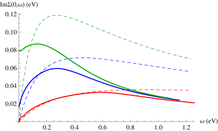
Figure 1: (Color online) Imaginary part of the zero-momentum self-energy, $\Sigma(0,\omega)$, for $n_{imp}=6\cdot 10^{12}$ cm^-2 and different densities, $n=6\cdot 10^{11}$, $1.7\cdot 10^{12}$, $6.7\cdot 10^{12}$ cm^-2, from top to bottom (solid lines). For comparison, the first order analytical result given by Eq. (20) is also plotted for the same values of the parameters (dashed lines).

Several features should be noted in Fig. 1. When $n_{imp}\ll n$, the SCBA result agree with the first order Born approximation result as expected. But when the impurity density is comparable with electron density, $n\simeq n_{imp}$, the disagreement between BA and SCBA is measurable, especially at high energies. When $n_{imp}$ is further increased ($n_{imp}>n$), the deviation becomes significant, and more interestingly a finite value of self energy is developed at zero energy, which gives rise to a finite density of states at the Dirac point (see below). The finite density of states at zero energy is one of the main characteristics of the SCBA result as compared to the first order Born approximation, which predicts a vanishing DOS at zero energy.

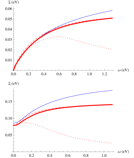
Figure 2: (Color online) Different approximations for the self-energy, at fixed impurity concentration of $6\cdot 10^{12}$ cm^-2, and for different electron densities, $6.7\cdot 10^{12}$ cm^-2 (upper panel) and $6\cdot 10^{11}$ cm^-2 (lower panel). The self-energies are: $\Sigma(k,\epsilon(k))$ (thick line), $\Sigma(k,k)$ (dashed line), $\Sigma(0,\omega)$ (dotted line). $\Sigma^{TF}(k,\epsilon(k))$, as computed with the Thomas-Fermi approximation, is shown for comparison in blue (upper curve).

As discussed in the introduction, the self-energy for the short range potentials does not depend on the wave vector. Therefore, the simple calculation at $k=0$ can be used for all wave vectors. However, when the self energy is a function of the wave vector and energy as for Coulomb disorder, the $k=0$ self-energy may be useful to analyze the physics near the Dirac point at high densities but, in general, it is not a good approximation to analyze it at finite wave vectors. Instead of zero wave vector self-energy, the most relevant value of the self-energy is at the on-shell self energy, $\Sigma(k,\epsilon(k))$, where the Green functions are peaked. A first approximation to the on-shell self-energy is obtained simply by taking $\Sigma(k,v_{F}k)$, but the true on-shell self-energy should be computed with the renormalized dispersion relation, $\Sigma(k,\epsilon(k))$ (this is only relevant when the dispersion relation is greatly changed by disorder).

The imaginary part of the three different self-energies $\Sigma(k,\epsilon(k)),\Sigma(k,v_{F}k),\Sigma(0,\omega)$ is displayed in Fig. 2 for two different impurity concentrations. We find that within SCBA the calculated self-energy for all different cases shows a finite value at the Dirac point for $n_{imp}>n$. Aside from this, we observe that the $k=0$ self-energy is indeed very different from the on-shell self energy. One should therefore be cautious when applying this approximation for general computations. We also observe that the true on-shell self-energy $\Sigma(k,\epsilon(k))$ presents almost no difference from the approximation $\Sigma(k,v_{F}k)$, which can thus be employed safely. Another approximation commonly used in the literature is to employ Thomas-Fermi screening for the Coulomb impurities instead of the full RPA dielectric function. We also show in Fig. 2 the imaginary part of self-energy $\Sigma(k,v_{F}k)$ with the TF screening function. A notable difference is observed compared with the RPA calculation. In particular, note that these two curves differ even for $\omega<2v_{F}k_{F}$.

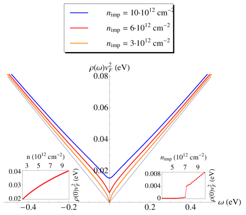
Figure 3: (Color online) Densities of states as a function of energy, for a fixed doping $n=1.6\cdot 10^{12}$ cm^-2, and varying impurity concentration, $n_{imp}=3\cdot 10^{12}$, $6\cdot 10^{12}$, $10\cdot 10^{12}$ cm^-2. The linear behavior for the clean case is shown for comparison (thin line) Left inset: Variation of the zero energy DOS upon simultaneous increase of $n$ and $n_{imp}$ (see text). Right inset: Zero energy DOS as a function of $n_{imp}$, for fixed doping of $n=3\cdot 10^{12}$ cm^-2.

The density of states of the system can be calculated with the self energy, Eq. (27). Fig. 3 shows the densities of states as a function of energy for a fixed electron density $n$ and several impurity concentrations. A significant finite value is observed at the Dirac point for high impurity concentrations, in agreement with the previous discussion on the self-energy. To quantify better where the onset of this finite value occurs, in the inset of Fig. 3 we show the DOS at the Dirac point as a function of $n_{imp}$, for $n=3\cdot 10^{12}$ cm^-2. A clear threshold is observed for a value of $\gamma\simeq 0.4$. This finite value of the density of states is also similar to the one obtained in the short range case. However, there is a significant difference. In the short range case, the analytical calculation predicts that this finite value is proportional to the cut-off, the only scale with dimensions at $\omega=0$. The density of states, therefore, remains constant if the rest of the scales in the problem are changed simultaneously. To check weather this behavior is present in the case of Coulomb impurities, we computed the zero energy density of states for $n_{imp}=6n$ sweeping the value of $n$. This is shown in the left inset of fig. 3. A clear monotonous behavior is observed, indicating a more complicated dependence on these scales than the constant behavior of the short range case.

Another spectral property of interest is the one particle relaxation time $\tau_{e}$, given as the inverse imaginary part of the on-shell self-energy at the Fermi level. Fig. 4 shows a plot of the dependence of $\tau_{e}$ with the Fermi level $k_{F}$ and the first order Born approximation results, Eq. (21). For each concentration of impurities, the fermi momentum $k_{F}=\alpha\sqrt{n_{imp}}$ which corresponds to $\gamma=1$ and separates the high and low doping region is plotted as a horizontal line. It is clearly seen that in the high doping region, the SCBA is again indistinguishable from the first order result. We also see how in the low doping region, deviations from the linear behavior are clearly identified.

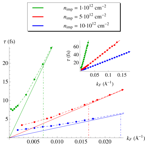
Figure 4: (Color online) One particle lifetime $\tau_{e}$ as a function of $k_{F}$, for different impurity concentrations (the physical value of $\hbar$ is restored in the units). The full line is the first order prediction given by Eq. (21). The dashed line is a guide to the eye. A vertical dotted-dashed line is plotted at the value $k_{F}=\alpha\sqrt{n_{imp}}$ which corresponds to $\gamma=1$, for each $n_{imp}$. Inset: Same plot for larger values of $k_{F}$, where the linear behavior predicted by Eq. (21) is fully appreciated.

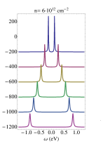
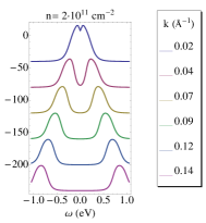
(a)

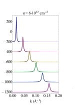
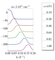
(b)

Figure 5: (Color online) a) EDC at a fixed impurity density of $3\cdot 10^{12}$ cm^-2, for two values of the doping $n=6\cdot 10^{12}$, $2\cdot 10^{11}$ cm^-2. b) MDCs for the same parameters. Note the change in absolute scale from left to right.

Finally, we discuss the spectral function of the system, given by Eq. (28). The spectral function is a physical magnitude that is directly measured in ARPES experiments BOM07 ; ZGF07 ; BOS07 ; SSH09 . A customary way of representing the spectral function is through two sets of plots: its constant $\omega$ sections as a function of $k$, known as momentum distribution curves (MDCs) and its constant $k$ sections as a function of $\omega$, known as energy distribution curves (EDCs). Here we show both of them in Fig. 5, for $n_{imp}=3\cdot 10^{12}$ cm^-2 and $n=2\cdot 10^{11}$ and $6\cdot 10^{12}$ cm^-2. We observe the typical broadening of the quasiparticle Lorentzian peaks due to disorder, whose width increases with increasing impurity density. However, a closer look reveals an unexpected feature. Fig. 6 shows the evolution of the MDCs with decreasing doping, and the best Lorentzian fit to each curve is also shown. It is appreciated that as doping is decreased the lineshapes become strongly non-Lorentzian. This is due to the momentum dependence of the self-energy: the MDCs are obtained from Eq. (29) by fixing the frequency. If the function $\Sigma(k)$ changes significantly from its on shell value $\Sigma(k_{0})$ (with $k_{0}$ defined by $\omega_{0}=\epsilon(k_{0})$) within a scale $\eta$, then regarding the MDCs, the self-energy looks like a constant if $\Sigma(k_{0},\omega_{0})<<\eta$, and therefore the MDC looks like a Lorentzian. Analyzing our numerical data, it can be seen that this condition is fulfilled only for small impurity concentrations, and this is the reason for the non-Lorentzian peaks shown in fig. 6.

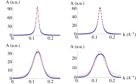
Figure 6: MDCs at fixed $\omega=0.8$ $eV$ for $n_{imp}=6\cdot 10^{12}$ cm^-2 and decreasing chemical potential $\mu=0.30$ eV (top left), $0.20$ eV (top right), $0.09$ eV (bottom left), $0.05$ eV (bottom right). The best Lorentzian fit to the data is shown in red. Note how the lineshape becomes manifestly non-Lorentzian as the doping is reduced.

IV.2 The optical conductivity

In this section we investigate the optical conductivity of graphene, which is affected strongly by long-range charged impurities. The optical conductivity of the ideal (or intrinsic) Dirac fermion model is predicted to be frequency independent and given by the universal value CGP09

$$\sigma_{0}\equiv\frac{\pi}{2}\frac{e^{2}}{h}.$$ (30)

This frequency independent optical conductivity has been measured in both suspended samples NBG08 and samples deposited on SiO₂ MSW08 . This universal result is observed even beyond the energies where the Dirac model is valid, due to the smallness of the correction induced by trigonal warping SPG08 . The absence of sizable electron-electron interaction corrections in these experiments has also been recently discussed HJV08 ; M08 ; SS09 . Moreover, this ideal picture may be modified by a thermal broadening or a level broadening of the single particle states due to disorder PGC06 ; RMF07 . In the presence of the broadenings the universal value Eq. (30) is obtained only in the asymptotically high energy limit, where all energy scale of broadenings are negligible.

Optical conductivity experiments have also been performed in the gated system LHJ08 ; HCG10 , where the optical conductivity with different electron densities has been studied. Theoretically, the optical conductivity at finite carrier density (or finite chemical potential $\mu$) has been addressed by many authors ASZ02 ; GSC06 ; PLS07 ; FP07a ; SPC08 ; GVV09 ; PRC10 ; P10a . Without any disorder and at $T=0$ the optical conductivity at finite density arises from two contributions: a Drude peak at zero energy from intraband transitions and a constant contribution from interband transitions, Eq. (30), starting at the threshold energy $\omega=2\mu$. However, in the real experiment LHJ08 , a number of strong deviations from these ideal predictions have been observed.p10a One of them is a constant background conductivity in the region between the Drude peak and the threshold at $\omega=2\mu$, where the interband optical transition is forbidden. An anomalously large energy broadening of the threshold has also been observed, which cannot be explained in terms of thermal broadening. This anomalous optical conductivity in the forbidden region has been attributed to various physical mechanisms. Short range impurities produce a broadening of both the Drude peak and the threshold ASZ02 , and more recently Coulomb impurities have been considered within Born approximation to produce a similar but stronger effect SPC08 . Electron-electron interactions are also considered to explain the background optical conductivity GVV09 ; PRC10 . In addition, the measured optical conductivity of very low mobility samples in CVD graphene HCG10 shows a reduction of the free carrier Drude weight induced by the intraband transition and consequently a substantial weight increase due to interband transition, which can not be explained within Born approximation.

While the effects of short-range scatterers on the optical conductivity have been computed in the SCBA ASZ02 , Coulomb impurities have only been considered within the first order Born approximation SPC08 . In this section we calculate the optical conductivity of graphene within the self-consistent Born approximation and provide the experimental relevance of our results. We use the Kubo formula with the SCBA self-energies calculated in the previous section. The optical conductivity can be computed from the current-current correlation function as

$$\sigma(\omega)=\frac{g_{s}g_{v}}{2\pi\omega}\int_{-\omega+\mu}^{\mu}dE\int kdk\sum_{ss^{\prime}}A_{s}(k,E)A_{s^{\prime}}(k,E+\omega)$$ (31)

with $A_{s}(k,\omega)$, the spectral function defined in Eq. (29).

Fig. 7 shows the optical conductivity as a function of energy for different electron densities with the full self-energies obtained from the self-consistent Born approximation. For comparison, the optical conductivity with the first order self-energy given by Eq. (20) is also shown. As expected, the result approaches to the value $\sigma_{0}$ for $\omega\gg 2\mu$. Most importantly, the SCBA result gives significantly more background conductivity for the density $n<n_{imp}$. We note that the four curves correspond to values of $\gamma$ = 0.63, 0.35, 0.22 and 0.16, for given chemical potentials of $\mu=$0.15, 0.20, 0.25, and 0.30 eV, respectively. As discussed in the previous section, SCBA effects are more significant for the low electron densities. The self-energy relevant for this computation is the on-shell self-energy, which is clearly different from the $k$=0 self-energy. In particular, it gives a non-zero broadening at the Dirac point, which is partially responsible for the background at $\omega$ close to $\mu$.

While these results improve on those computed with the first order self-energy for $n_{imp}>n$, , they also indicate that Coulomb impurities are not the only contribution in the experiment in LHJ08 . Indeed, any scattering mechanism which is affected by screening will tend to produce less scattering as the doping is increased, and what is needed to explain the background in the forbbiden region is a mechanism which becomes more efficient at high dopings. Our results are consistent, however, with the latest experiment reported in HCG10 , which seems to be dominated mainly by disorder.

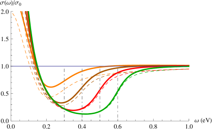
Figure 7: Real part of the optical conductivity for a impurity density $n_{imp}=6\cdot 10^{12}$ cm^-2 and several chemical potentials $\mu=0.15$, $0.20$, $0.25$, $0.30$ eV. The solid (dashed) lines indicate the optical conductivities calculated with the SCBA self-energy (with the first order self-energy at $k=0$). The corresponding values for $\gamma$ for each curve are 0.63, 0.35, 0.22 and 0.16.

V Discussion and conclusions

We now discuss several aspects of the results shown in the previous sections. We have shown that the $k=0$ self-energy widely employed for the electron self-energy is only valid near the Dirac point and very different from the on-shell self-energy. Thus it is necessary to consider the on-shell self energy to describe the electronic properties of disordered graphene. The on-shell self-energy with bare single particle energy is not much different from the true self-energy and represents a reasonable approximation. We also discuss the Thomas-Fermi (TF) screening approximation and its relation with the RPA approximation. Since the TF screening function is equivalent to the RPA result for $k<2k_{F}$, it seems that the self-energies calculated within both approximations should coincide at low energies. However, as shown in Fig. 2 the TF self-energy differs from its RPA counterpart at all energies. The difference becomes greater at higher values of $\gamma$ as defined in Eq. (26), especially for high impurity concentrations. This is because the SCBA is non-local in momentum space and the difference between TF and RPA at high momenta is enough to alter the low-energy region of the self-energy. It is therefore more reliable to use the RPA screening function even for $\omega<2v_{F}k_{F}$.

We now compare our SCBA results with those obtained in the same approximation for short range disorder HHD08 ; PGC06 . We find that even though the densities of states for both cases are similar in energy dependence at low impurity densities the dependence of both $n$ and $n_{imp}$ is very different. We also find that the single particle relaxation time behaves very differently depending on whether $\gamma>1$ or $\gamma<1$. The parameter $\gamma$ determines to what extent the SCBA differs from the first order Born approximation. It is a good consistency test that for small values of $\gamma$, our numerical integration results match perfectly with the first order Born approximation Eq. (21). This allows us to see clearly the deviation from linearity as the disorder density increases. This deviation is characteristic of Coulomb impurities which gives rise to the ratio $\tau_{tr}/\tau_{e}$ to deviate from its constant value at low impurity densities.

The momentum distribution curves (MDC) calculated within the self-consistence Born approximation have also revealed an unexpected feature. They become non-Lorentzian with decreasing electron density, which suggests that the evolution of MDCs with density could be used to probe the relevant scattering mechanisms in graphene. If the MDC become non-Lorentzian by lowering the electron density, this is a signature of a momentum dependent self-energy, which could be produced by Coulomb impurities (other momentum-dependent potentials such as ripples could perhaps produce a similar effect, but the method is still useful to distinguish short range scatterers from long range scatterers).

Finally, the discussed spectral features have a direct influence on the optical conductivity. We have shown that long range Coulomb impurities beyond the Born approximation induce a characteristic broadening in the shape of the optical conductivity at finite doping compatible with recent experiments.

In summary, this work has addressed the effects of long ranged charged impurities on the electronic properties of graphene, showing how self-consistent scheme modifies them as the impurity density $n_{imp}$ is increased. The SCBA in the presence of Coulomb disorder produces characteristic features in both the spectral properties and the optical conductivity which may be relevant in the explanation of current experiments.

VI Acknowledgments

We would like to thank A.G. Grushin and E.V. Castro for very useful discussions. F.J. was supported by the I3P predoctoral program from CSIC and from MICINN (Spain) through grant FIS2008-00124. EHH acknowledges a financial support from US-ONR-MURI.

References

- (1) K. S. Novoselov, A. K. Geim, S. V. Morozov, D. Jiang, Y. Zhang, S. V. Dubonos, I. V. Grigorieva, and A. A. Firsov, Science 306, 666 (2004)
- (2) K. S. Novoselov, A. K. Geim, S. V. Morozov, D. Jiang, M. I. Katsnelson, I. V. Grigorieva, S. V. Dubonos, and A. A. Firsov, Nature 438, 197 (2005)
- (3) A. H. Castro Neto, F. Guinea, N. M. R. Peres, K. S. Novoselov, and A. K. Geim, Rev. Mod. Phys. 81, 109 (2009)
- (4) A. K. Geim, Science 324, 1530 (2009)
- (5) N. M. R. Peres, J. Phys.: Condens. Matter 21, 323201 (2009)
- (6) D. S. L. Abergel, V. Apalkov, J. Berashevich, K. Ziegler, and T. Chakraborty, cond-mat/1003.0391
- (7) S. Das Sarma, S. Adam, E. H. Hwang, and E. Rossi, cond-mat/1003.4731
- (8) E. R. Mucciolo and C. H. Lewenkopf, J. Phys.: Condens. Matter 22, 273201 (2010)
- (9) T. Ando, J. Phys. Soc. Jpn 75, 074716 (2006)
- (10) E. H. Hwang, S. Adam, and S. Das Sarma, Phys. Rev. Lett. 98, 186806 (2007)
- (11) V. V. Cheianov and V. I. Fal’ko, Phys. Rev. Lett. 97, 226801 (2006)
- (12) K. Nomura and A. H. MacDonald, Phys. Rev. Lett. 96, 256602 (2006)
- (13) T. Stauber, N. M. R. Peres, and F. Guinea, Phys. Rev. B 76, 205423 (2007)
- (14) M. I. Katsnelson and A. K. Geim, Phil. Trans. R. Soc. A 366, 195 (2008)
- (15) Z. H. Ni, L. A. Ponomarenko, R. R. Nair, R. Yang, S. Anissimova, I. V. Grigorieva, F. Schedin, Z. X. Shen, E. H. Hill, K. S. Novoselov, and A. K. Geim, cond-mat/1003.0202
- (16) Y. Tan, Y. Zhang, K. Bolotin, Y. Zhao, S. Adam, E. H. Hwang, S. Das Sarma, H. L. Stormer, and P. Kim, Phys. Rev. Lett. 99, 246803 (2007)
- (17) K. Nomura and A. H. MacDonald, Phys. Rev. Lett. 98, 076602 (2007)
- (18) N. M. R. Peres, Rev. Mod. Phys. 82, 2673 (2010)
- (19) E. H. Hwang and S. Das Sarma, Phys. Rev. B 77, 195412 (2008)
- (20) X. Hong, K. Zou, and J. Zhu, Phys. Rev. B 80, 241415 (2009)
- (21) M. Monteverde, C. Ojeda-Aristizabal, R. Weil, K. Bennaceur, M. Ferrier, S. Guéron, C. Glattli, H. Bouchiat, J. N. Fuchs, and D. L. Maslov, Phys. Rev. Lett. 104, 126801 (2010)
- (22) Y. Zhang, V. W. Brar, C. Girit, A. Zettl, and M. F. Crommie, Nature Phys. 5, 722 (2009)
- (23) F. de Juan, A. Cortijo, and M. A. H. Vozmediano, Phys. Rev. B 76, 165409 (2007)
- (24) S. Y. Zhou, G. Gweon, A. V. Fedorov, P. N. First, W. A. de Heer, D. Lee, F. Guinea, A. H. Castro Neto, and A. Lanzara, Nature Mat. 6, 770 (2007)
- (25) A. Bostwick, T. Ohta, T. Seyller, K. Horn, and E. Rotenberg, Nature Phys. 3, 36 (2007)
- (26) K. R. Knox, S. Wang, A. Morgante, D. Cvetko, A. Locatelli, T. O. Mentes, M. A. Niño, P. Kim, and R. M. Osgood, Phys. Rev. B 78, 201408 (2008)
- (27) Z. Q. Li, E. A. Henriksen, Z. Jiang, Z. Hao, M. C. Martin, P. Kim, H. L. Stormer, and D. N. Basov, Nature Phys. 4, 532 (2008)
- (28) J. Horng, C. Chen, B. Geng, C. Girit, Y. Zhang, Z. Hao, H. A. Bechtel, M. Martin, A. Zettl, M. F. Crommie, Y. R. Shen, and F. Wang, cond-mat/1007.4623
- (29) T. Stauber, N. M. R. Peres, and A. H. Castro Neto, Phys. Rev. B 78, 085418 (2008)
- (30) J. Rammer, Quantum transport theory (Westview Press, 1998)
- (31) A. Qaiumzadeh, N. Arabchi, and R. Asgari, Solid State Commun. 147, 172 (2008)
- (32) X. Yan and C. S. Ting, Phys. Rev. Lett. 101, 126801 (2008)
- (33) X. Yan, Y. Romiah, and C. S. Ting, Phys. Rev. B 77, 125409 (2008)
- (34) D. P. DiVincenzo and E. J. Mele, Phys. Rev. B 29, 1685 (1984)
- (35) M. M. Fogler, D. S. Novikov, and B. I. Shklovskii, Phys. Rev. B 76, 233402 (2007)
- (36) I. S. Terekhov, A. I. Milstein, V. N. Kotov, and O. P. Sushkov, Phys. Rev. Lett. 100, 076803 (2008)
- (37) M. I. Katsnelson, Phys. Rev. B 74, 201401 (2006)
- (38) A. V. Shytov, M. I. Katsnelson, and L. S. Levitov, Phys. Rev. Lett. 99, 236801 (2007)
- (39) R. R. Biswas, S. Sachdev, and D. T. Son, Phys. Rev. B 76, 205122 (2007)
- (40) V. M. Pereira, J. Nilsson, and A. H. Castro Neto, Phys. Rev. Lett. 99, 166802 (2007)
- (41) M. Ghaznavi, Z. L. Miskovic, and F. O. Goodman, cond-mat/0910.3614
- (42) T. Ando, A. B. Fowler, and F. Stern, Rev. Mod. Phys. 54, 437 (1982)
- (43) E. Zaremba, I. Nagy, and P. M. Echenique, Phys. Rev. Lett. 90, 046801 (2003)
- (44) S. Gangadharaiah, A. M. Farid, and E. G. Mishchenko, Phys. Rev. Lett. 100, 166802 (2008)
- (45) S. Das Sarma, B. Y. Hu, E. H. Hwang, and W. Tse, cond-mat/0708.3239
- (46) E. H. Hwang and S. Das Sarma, Phys. Rev. B 75, 205418 (2007)
- (47) M. van Schilfgaarde and M. I. Katsnelson, cond-mat/1006.2426
- (48) L. Brey and H. A. Fertig, Phys. Rev. B 80, 035406 (2009)
- (49) A. L. Efros, Solid State Commun. 65, 1281 (1988)
- (50) B. Y. Hu, E. H. Hwang, and S. Das Sarma, Phys. Rev. B 78, 165411 (2008)
- (51) N. M. R. Peres, F. Guinea, and A. H. Castro Neto, Phys. Rev. B 73, 125411 (2006)
- (52) C. H. Yang, F. M. Peeters, and W. Xu, Phys. Rev. B 82, 075401 (2010)
- (53) A. A. Nersesyan, A. M. Tsvelik, and F. Wenger, Nucl. Phys. B 438, 561 (1995)
- (54) I. L. Aleiner and K. B. Efetov, Phys. Rev. Lett. 97, 236801 (2006)
- (55) E. Fradkin, Phys. Rev. B 33, 3263 (1986)
- (56) A. Altland, B. D. Simons, and M. R. Zirnbauer, Phys. Rep. 359, 283 (2002)
- (57) D. V. Khveshchenko, Phys. Rev. B 75, 241406 (2007)
- (58) J. Chen, C. Jang, S. Adam, M. S. Fuhrer, E. D. Williams, and M. Ishigami, Nature Phys. 4, 377 (2008)
- (59) A. Bostwick, T. Ohta, J. L. McChesney, T. Seyller, K. Horn, and E. Rotenberg, Solid State Commun. 143, 63 (2007)
- (60) M. Sprinkle, D. Siegel, Y. Hu, J. Hicks, A. Tejeda, A. Taleb-Ibrahimi, P. Le Fèvre, F. Bertran, S. Vizzini, H. Enriquez, S. Chiang, P. Soukiassian, C. Berger, W. de Heer, A. Lanzara, and E. Conrad, Phys. Rev. Lett. 103, 226803 (2009)
- (61) R. R. Nair, P. Blake, A. N. Grigorenko, K. S. Novoselov, T. J. Booth, T. Stauber, N. M. R. Peres, and A. K. Geim, Science 320, 1308 (2008)
- (62) K. F. Mak, M. Y. Sfeir, Y. Wu, C. H. Lui, J. A. Misewich, and T. F. Heinz, Phys. Rev. Lett. 101, 196405 (2008)
- (63) T. Stauber, N. M. R. Peres, and A. K. Geim, Phys. Rev. B 78, 085432 (2008)
- (64) I. F. Herbut, V. Juričić, O. Vafek, and M. J. Case, cond-mat/0809.0725
- (65) E. G. Mishchenko, Europhys. Lett. 83, 17005 (2008)
- (66) D. E. Sheehy and J. Schmalian, Phys. Rev. B 80, 193411 (2009)
- (67) S. Ryu, C. Mudry, A. Furusaki, and A. W. W. Ludwig, Phys. Rev. B 75, 205344 (2007)
- (68) V. P. Gusynin, S. G. Sharapov, and J. P. Carbotte, Phys. Rev. Lett. 96, 256802 (2006)
- (69) N. M. R. Peres, J. M. B. Lopes dos Santos, and T. Stauber, Phys. Rev. B 76, 073412 (2007)
- (70) L. A. Falkovsky and S. S. Pershoguba, Phys. Rev. B 76, 153410 (2007)
- (71) A. G. Grushin, B. Valenzuela, and M. A. H. Vozmediano, Phys. Rev. B 80, 155417 (2009)
- (72) N. M. R. Peres, R. M. Ribeiro, and A. H. Castro Neto, Phys. Rev. Lett. 105, 055501 (2010)