Critical behavior of non-intersecting Brownian motions at a tacnode

Abstract

We study a model of $n$ one-dimensional non-intersecting Brownian motions with two prescribed starting points at time $t=0$ and two prescribed ending points at time $t=1$ in a critical regime where the paths fill two tangent ellipses in the time-space plane as $n\to\infty$. The limiting mean density for the positions of the Brownian paths at the time of tangency consists of two touching semicircles, possibly of different sizes. We show that in an appropriate double scaling limit, there is a new familiy of limiting determinantal point processes with integrable correlation kernels that are expressed in terms of a new Riemann-Hilbert problem of size $4\times 4$. We prove solvability of the Riemann-Hilbert problem and establish a remarkable connection with the Hastings-McLeod solution of the Painlevé II equation. We show that this Painlevé II transcendent also appears in the critical limits of the recurrence coefficients of the multiple Hermite polynomials that are associated with the non-intersecting Brownian motions. Universality suggests that the new limiting kernels apply to more general situations whenever a limiting mean density vanishes according to two touching square roots, which represents a new universality class.

Keywords: non-intersecting Brownian motion, determinantal point process, correlation kernel, Riemann-Hilbert problem, Deift-Zhou steepest descent analysis, Painlevé II equation, multiple Hermite polynomial.

1 Introduction

In recent years the model of non-intersecting Brownian motions has been studied in various regimes, see e.g. [2, 6, 19, 20, 33, 34, 35, 44], where many connections with determinantal point processes and random matrix theory were found, see also [32, 37, 36, 44] for non-intersecting Bessel paths and Brownian excursions. Their discrete counterparts, the non-intersecting random walks, have important connections with tiling and random growth models, see e.g. [8, 12, 28, 29, 42].

In this paper we consider one-dimensional non-intersecting Brownian motions with two prescribed starting points at time $t=0$ and two prescribed ending points at time $t=1$. We assume that the number of paths that leave from the topmost (bottommost) starting point is the same as the number of paths that arrive at the topmost (bottommost) ending point. As the number of paths increases and simultaneously the overall variance of the Brownian transition probability decreases, we may create various situations that are illustrated in Figure 1.

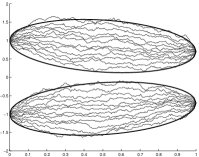
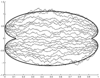
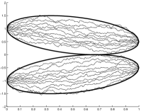
Figure 1: Non-intersecting Brownian motions with two starting and two ending positions in case of (a) large, (b) small, and (c) critical separation between the endpoints. Here the horizontal axis denotes the time, $t\in[0,1]$, and for each fixed $t$ the positions of the $n$ non-intersecting Brownian motions at time $t$ are denoted on the vertical line through $t$. Note that for $n\to\infty$ the positions of the Brownian motions fill a prescribed region in the time-space plane, which is bounded by the boldface lines in the figures. Here we have chosen $N=n=20$ and $p_{1}=p_{2}=1/2$ in each of the figures, and (a) $a_{1}=-a_{2}=1$, $b_{1}=-b_{2}=0.7$, (b) $a_{1}=-a_{2}=0.4$, $b_{1}=-b_{2}=0.3$, and (c) $a_{1}=-a_{2}=1$, $b_{1}=-b_{2}=1/2$, in the cases of large, small and critical separation, respectively.

In case of large separation of the starting and ending points we have a situation as in Figure 1(a). The paths are in two disjoint groups, where one group of paths goes from the topmost starting point to the topmost ending point, and the other group goes from the bottommost starting point to the bottommost ending point. In the large $n$ limit the paths fill out two disjoint ellipses.

In case of small separation of the starting and ending points we have a situation as in Figure 1(b). Here the two groups of paths that emanate from the two starting points merge at a certain time, stay together for a while, and separate at a later time. In the large $n$ limit the paths fill out a region that is bounded by a more complicated curve with two cusp points. The critical behavior at the cusp point is known to be described by the Pearcey process, see [5, 9, 41, 44].

In the transitional case of critical separation the paths fill out two ellipses that are tangent at a critical time as shown in Figure 1(c). The case of critical separation was already considered by the first two authors [19], but at the non-critical time. Here we consider the behavior at the critical time. Note that the tangent point of two ellipses is called a tacnode in the classification scheme of singular points of algebraic curves, whence the title of this paper; see also [11] where another model is analyzed with a tacnode, but with markedly different properties.

The phase transition at critical separation can already be observed at times different from the critical time $t_{\textrm{crit}}$. In [19] a connection was found with the Hastings-McLeod solution of the Painlevé II equation

$$q^{\prime\prime}(s)=sq(s)+2q^{3}(s).$$ (1.1)

Here the prime denotes the derivative with respect to $s$. The Hasting-McLeod solution [26] is the special solution $q(s)$ of (1.1), which is real for real $s$ and satisfies

$$q(s)=\mathrm{Ai}(s)(1+o(1)),\qquad\text{as }s\to+\infty,$$ (1.2)

where $\mathrm{Ai}$ denotes the usual Airy function.

The Hastings-McLeod solution $q(s)$ (or functions related to it) do not appear in the local scaling limits of the correlation kernel at time $t\neq t_{\textrm{crit}}$. The Hastings-McLeod solution, however, does appear in the asymptotics of the recurrence coefficients of the multiple Hermite polynomials related to the non-intersecting Brownian motions, see [19].

The results in [19] were obtained from the Deift-Zhou steepest descent analysis of the $4\times 4$ matrix-valued Riemann-Hilbert (RH) problem for multiple Hermite polynomials. During the analysis we had to construct a local parametrix at a point $x_{0}\in\mathbb{R}$ that lies strictly between the two intervals where the two groups of Brownian paths accumulate. The point $x_{0}$ does not have a physical meaning. However, the local parametrix affects the recurrence coefficients of the multiple Hermite polynomials, as mentioned before.

The aim of this paper is to perform a similar steepest descent analysis for the critical time $t=t_{\textrm{crit}}$. This multicritical situation, after appropriate scaling of the parameters will be locally described by the solution of a model RH problem of size $4\times 4$. The RH problem can be considered as a combination of two RH problems for the Airy function with an additional non-trivial coupling in the jump matrices.

Using this new $4\times 4$ model RH problem, we obtain an expression for the limit of the correlation kernel at the critical time. We show that the kernel has an integrable form determined by the solution to the RH problem, see Theorem 2.7.

We find it remarkable that this new $4\times 4$ RH problem is again related to the Hastings-McLeod solution of the Painlevé II equation. More precisely, we prove that the Hastings-McLeod solution shows up in the residue matrix in the asymptotic series at infinity of the $4\times 4$ model RH problem, see Theorem 2.4. This is very similar to the situation for the classical $2\times 2$ RH problem for Painlevé II due to Flaschka-Newell [22, 23]. This suggests that our $4\times 4$ problem may be expressible in terms of this smaller $2\times 2$ problem; however we could not find such an expression. So our RH problem might lead to a genuinely new Lax pair for the Hastings-McLeod solution to Painlevé II. See also the paper [30] for Lax pairs with matrices of size $3\times 3$.

As a consequence, we are able to show that the results in [19] on the recurrence coefficients remain valid at the critical time $t=t_{\textrm{crit}}$, i.e., the asymptotic behavior of the recurrence coefficients of the multiple Hermite polynomials is still governed by the Hastings-McLeod solution to Painlevé II with exactly the same formulas as in [19]. We find this a surprising fact.

Very recently, a model of non-intersecting random walks was studied by Adler, Ferrari and Van Moerbeke [4] in a situation that is very similar to ours. There are two groups or random walks in [4], that in the scaling limit fill out two domains that are tangent in one point. It is shown that there is a limiting correlation kernel at the tacnode, and two expressions for it are given in terms of multiple integrals involving Airy functions and the Airy kernel resolvent. It seems very likely that this limiting kernel should be equivalent to the one that we obtain in Theorem 2.7 below for the symmetric case (i.e., $p_{1}^{*}=p_{2}^{*}=1/2$ in Theorem 2.7), but we have not been able to make this identification.

It would indeed be interesting to see how the Painlevé II equation arises in the framework of [4], and conversely, to see how our formula can be reduced to integrals with Airy functions and the Airy kernel resolvent. It would also be interesting to have a process version with an extended tacnode kernel.

2 Statement of results

We now give a precise statement of our results. In Sections 2.1-2.3 we describe our situation and the connection with a $4\times 4$ matrix valued RH problem. In Section 2.4 we formulate the the new $4\times 4$ RH problem and its properties, in particular the connection with the Painlevé II equation. Finally, in Sections 2.5–2.6 we state the main results about the limiting behavior of the correlation kernels and recurrence coefficients.

2.1 Correlation kernel and the Riemann-Hilbert problem

We consider $n$ one-dimensional non-intersecting Brownian motions with two starting points $a_{1}>a_{2}$ at time $t=0$ and two ending points $b_{1}>b_{2}$ at time $t=1$. We assume that $n_{1}$ of the particles move from the topmost starting point $a_{1}$ to the topmost ending point $b_{1}$, and $n_{2}$ particles move from the bottommost starting point $a_{2}$ to the bottommost ending point $b_{2}$, with $n_{1}+n_{2}=n$.

The transition probability density of the Brownian motions is

$$P_{N}(t,x,y)=\frac{1}{\sqrt{2\pi t}\,\sigma_{N}}\exp\left(-\frac{1}{2t\sigma_{N}^{2}}(x-y)^{2}\right),\qquad\sigma_{N}^{2}=1/N,$$ (2.1)

with an overall variance $\sigma_{N}^{2}=1/N$, that decreases as $n$ increases such that

$$T=n\sigma_{N}^{2}=\frac{n}{N}>0$$ (2.2)

remains fixed. We interpret $T$ as a temperature variable.

Using the above setting, it is known that the positions $x_{1},\ldots,x_{n}$ of the Brownian paths at time $t\in(0,1)$ have a joint probability density [31]

$$p(x_{1},\ldots,x_{n})=\frac{1}{Z_{n}}\det\left(f_{i}(x_{j})\right)_{i,j=1}^{n}\,\det\left(g_{i}(x_{j})\right)_{i,j=1}^{n}$$ (2.3)

with functions

$$f_{i}(x) =\frac{\partial^{i-1}}{\partial x^{i-1}}P_{N}(t,a_{1},x),\qquad i=1,\ldots,n_{1},$$ (2.4)

$$f_{n_{1}+i}(x) =\frac{\partial^{i-1}}{\partial x^{i-1}}P_{N}(t,a_{2},x),\qquad i=1,\ldots,n_{2},$$ (2.5)

$$g_{i}(x) =\frac{\partial^{i-1}}{\partial x^{i-1}}P_{N}(1-t,x,b_{1}),\qquad i=1,\ldots,n_{1},$$ (2.6)

$$g_{n_{1}+i}(x) =\frac{\partial^{i-1}}{\partial x^{i-1}}P_{N}(1-t,x,b_{2}),\qquad i=1,\ldots,n_{2},$$ (2.7)

and with $Z_{n}$ a normalization constant. Note that (2.3) is a biorthogonal ensemble [10]. In particular, it is a determinantal point process with correlation kernel

$$K_{n}(x,y)=\sum_{i,j=1}^{n}f_{i}(x)\left(A^{-1}\right)_{i,j}g_{j}(y),$$ (2.8)

where $\left(A^{-1}\right)_{i,j}$ denotes the $(i,j)$th entry of the inverse of the matrix

$$A=\left(\int_{\mathbb{R}}f_{i}(x)g_{j}(x)dx\right)_{i,j=1}^{n}.$$

The double sum formula (2.8) for the kernel is not very tractable for asymptotic analysis. However there is a convenient representation of $K_{n}$ in terms of the solution of a Riemann-Hilbert problem. It is of size $4\times 4$, since $4$ is the total number of starting and ending positions.

Define the weight functions

$$w_{1,k}(x) =\exp\left(-\frac{n}{2Tt}(x^{2}-2a_{k}x)\right), k=1,2,$$ (2.9)

$$w_{2,l}(x) =\exp\left(-\frac{n}{2T(1-t)}(x^{2}-2b_{l}x)\right), l=1,2,$$ (2.10)

and consider the following RH problem which was introduced in [14] as a generalization of the RH problem for orthogonal polynomials [24], see also [45].

RH problem 2.1.

We look for a $4\times 4$ matrix-valued function $Y:\mathbb{C}\setminus\mathbb{R}\to\mathbb{C}^{4\times 4}$ satisfying

1. $Y(z)$ is analytic for $z\in\mathbb{C}\setminus\mathbb{R}$.

2. $Y$ has limiting values $Y_{\pm}$ on $\mathbb{R}$, where $Y_{+}$ ($Y_{-}$) denotes the limiting value from the upper (lower) half-plane, and

   $$Y_{+}(x)=Y_{-}(x)\begin{pmatrix}I_{2}&W(x)\\ 0&I_{2}\end{pmatrix},\qquad x\in\mathbb{R},$$ (2.11)

   where $I_{2}$ denotes the $2\times 2$ identity matrix, and $W(x)$ is the rank-one matrix (outer product of two vectors)

   $$W(x)=\begin{pmatrix}w_{1,1}(x)\\ w_{1,2}(x)\end{pmatrix}\begin{pmatrix}w_{2,1}(x)&w_{2,2}(x)\end{pmatrix}.$$ (2.12)

3. As $z\to\infty$, we have that

   $$Y(z)=\left(I+\frac{Y_{1}}{z}+O\left(\frac{1}{z^{2}}\right)\right)\operatorname{diag}(z^{n_{1}},z^{n_{2}},z^{-n_{1}},z^{-n_{2}}).$$ (2.13)

The RH problem has a unique solution that can be described in terms of certain multiple orthogonal polynomials (actually multiple Hermite polynomials of mixed type), see [14, 19] for details. According to [14], the correlation kernel $K_{n}$ from (2.8) is equal to

$$K_{n}(x,y)=\frac{1}{2\pi i(x-y)}\begin{pmatrix}0&0&w_{2,1}(y)&w_{2,2}(y)\end{pmatrix}Y_{+}^{-1}(y)Y_{+}(x)\begin{pmatrix}w_{1,1}(x)\\ w_{1,2}(x)\\ 0\\ 0\end{pmatrix}.$$ (2.14)

The kernel $K_{n}$ in (2.14) not only depends on $n$, but also on $n_{1}$, $n_{2}$, $a_{1},a_{2}$, $b_{1},b_{2}$, $t$ and $T$. In what follows, we will take the variables $T$ and $t$ fixed while the other variables will be varying with $n$, see Section 2.3.

2.2 Separation of the starting and ending points

We now discuss in more detail the three situations in Figure 1. Given $n_{1}$ and $n_{2}$, we denote the corresponding fractions of particles by

$$p_{1}:=\frac{n_{1}}{n},\qquad p_{2}:=\frac{n_{2}}{n}=1-p_{1},$$ (2.15)

which are varying with $n$, and we assume that

$$p_{1}=p_{1}^{*}+O(1/n),\qquad p_{2}=p_{2}^{*}+O(1/n),\qquad n\to\infty,$$ (2.16)

for certain limiting values $p_{1}^{*},p_{2}^{*}\in(0,1)$. Of course, $p_{2}^{*}=1-p_{1}^{*}$.

For given $T$ and $p_{1}^{*},p_{2}^{*}$, the three cases of large, small and critical separation of the starting and ending points are distinguished as follows; see [19]. There is large separation in case the inequality

$$(a_{1}-a_{2})(b_{1}-b_{2})>T\left(\sqrt{p_{1}^{*}}+\sqrt{p_{2}^{*}}\right)^{2}$$ (2.17)

holds. Then the Brownian motion paths remain in two separate groups, and the limiting hull in the $tx$-plane consists of two ellipses. For any $t\in(0,1)$, the limiting distribution of the positions of the paths at time $t$ is supported on the two disjoint intervals $[\alpha_{1}^{*},\beta_{1}^{*}]$ and $[\alpha_{2}^{*},\beta_{2}^{*}]$, where the endpoints satisfy

$$\alpha_{2}^{*}<\beta_{2}^{*}<\alpha_{1}^{*}<\beta_{1}^{*}$$ (2.18)

and are given explicitly by

$$\alpha_{j}^{*}=(1-t)a_{j}+tb_{j}-2\sqrt{p_{j}^{*}Tt(1-t)},$$ (2.19)

$$\beta_{j}^{*}=(1-t)a_{j}+tb_{j}+2\sqrt{p_{j}^{*}Tt(1-t)},$$ (2.20)

with the limiting density on these intervals given by the semicircle laws

$$\frac{1}{2\pi Tt(1-t)}\sqrt{(\beta_{j}^{*}(t)-x)(x-\alpha_{j}^{*}(t))},\qquad x\in[\alpha_{j}^{*}(t),\beta_{j}^{*}(t)],$$ (2.21)

for $j=1,2$. See again Figure 1(a).

We are in the case of small separation if the inequality (2.17) is reversed, so that

$$(a_{1}-a_{2})(b_{1}-b_{2})<T\left(\sqrt{p_{1}^{*}}+\sqrt{p_{2}^{*}}\right)^{2}.$$ (2.22)

Then the limiting hull in the $tx$-plane is an algebraic curve and the limiting distribution of the paths at any given time $t\in(0,1)$ is not given by semicircle laws anymore. This was shown in [15] for the case where $p_{1}^{*}=p_{2}^{*}=1/2$. See Figure 1(b).

The case of critical separation corresponds to the equality sign in (2.17), that is,

$$(a_{1}-a_{2})(b_{1}-b_{2})=T\left(\sqrt{p_{1}^{*}}+\sqrt{p_{2}^{*}}\right)^{2}.$$ (2.23)

Then the limiting distribution is still given by two semicircle densities (2.21), which are now however touching at the critical time $t_{\textrm{crit}}\in(0,1)$ defined by

$$t_{\textrm{crit}}=\frac{a_{1}-a_{2}}{(a_{1}-a_{2})+(b_{1}-b_{2})},$$ (2.24)

in the sense that $\beta_{2}^{*}=\alpha_{1}^{*}$ in (2.18) when $t=t_{\textrm{crit}}$. See Figure 1(c).

2.3 Double scaling limit

In order to study the case of critical separation we choose without loss of generality

$$T=1,$$ (2.25)

and take $a_{1}^{*}>a_{2}^{*}$, $b_{1}^{*}>b_{2}^{*}$ so that

$$(a_{1}^{*}-a_{2}^{*})(b_{1}^{*}-b_{2}^{*})=\left(\sqrt{p_{1}^{*}}+\sqrt{p_{2}^{*}}\right)^{2},$$ (2.26)

cf. (2.23). We also take

$$t=t_{\textrm{crit}}=\frac{a_{1}^{*}-a_{2}^{*}}{(a_{1}^{*}-a_{2}^{*})+(b_{1}^{*}-b_{2}^{*})}$$ (2.27)

and

$$x_{\textrm{crit}}=(1-t_{\textrm{crit}})\frac{a_{1}^{*}+a_{2}^{*}}{2}+t_{\textrm{crit}}\frac{b_{1}^{*}+b_{2}^{*}}{2}$$ (2.28)

as the critical time and place of tangency.

We can assume that $T$ and $t$ remain fixed as in (2.25) and (2.27) without loss of generality, since we cannot create different limiting behavior by varying $T$ and $t$ as well, see Remarks 2.11 and 2.12 in Section 2.5.

We let the starting points $a_{1}$, $a_{2}$ and ending points $b_{1}$, $b_{2}$ be varying with $n$ in such a way that for certain real constants $L_{1},L_{2},L_{3},L_{4}$,

$$a_{1} =a_{1}^{*}+L_{1}n^{-2/3},\quad b_{1} =b_{1}^{*}+L_{3}n^{-2/3},$$ (2.29)

$$a_{2} =a_{2}^{*}+L_{2}n^{-2/3},\quad b_{2} =b_{2}^{*}+L_{4}n^{-2/3},$$ (2.30)

as $n\to\infty$. It turns out that the constants only appear in our results through the combinations

$$L_{5} :=(b_{1}^{*}-b_{2}^{*})L_{1}+(a_{1}^{*}-a_{2}^{*})L_{3},$$ (2.31)

$$L_{6} :=(b_{1}^{*}-b_{2}^{*})L_{2}+(a_{1}^{*}-a_{2}^{*})L_{4}.$$ (2.32)

Near the critical value $x_{\textrm{crit}}$, the asymptotics of $K_{n}$ for $n\to\infty$ will be described by a family of limiting kernels

$$K^{tacnode}(u,v;r_{1},r_{2},s_{1},s_{2}),\qquad u,v\in\mathbb{R},$$

depending on four variables $r_{1},r_{2}>0$ and $s_{1},s_{2}\in\mathbb{R}$ that depend on the values $p_{1}^{*}$, $p_{2}^{*}$, $L_{5}$ and $L_{6}$. Because of a dilation and translation symmetry

$$c^{2}K^{tacnode}(c^{2}u,c^{2}v;r_{1},r_{2},s_{1},s_{2})=K^{tacnode}(u,v;c^{3}r_{1},c^{3}r_{2},cs_{1},cs_{2}),\qquad c>0,$$

$$K^{tacnode}(u+2c,v+2c;r_{1},r_{2},s_{1},s_{2})=K^{tacnode}(u,v;r_{1},r_{2},s_{1}-cr_{1},s_{2}+cr_{2}),\qquad c\in\mathbb{R},$$

the family essentially depends on two parameters only, and we could for example choose $r_{1}=1$, $s_{1}=s_{2}$. However, in order to preserve the symmetry in the formulas, we prefer to use four parameters.

The limiting kernels are given in terms of a RH problem that we discuss next.

2.4 A new $4\times 4$ Riemann-Hilbert problem

The $4\times 4$ matrix-valued RH problem has jumps on a contour in the complex plane consisting of $10$ rays emanating from the origin. The rays are determined by two numbers $\varphi_{1},\varphi_{2}$ such that

$$0<\varphi_{1}<\varphi_{2}<\pi/3.$$ (2.33)

The value $\pi/3$ in (2.33) is not the optimal one, but it will be sufficient for our purposes. We define the half-lines $\Gamma_{k}$, $k=0,\ldots,9$, by

$$\Gamma_{0}=\mathbb{R}^{+},\qquad\Gamma_{1} =e^{i\varphi_{1}}\mathbb{R}^{+}, \qquad\Gamma_{2}=e^{i\varphi_{2}}\mathbb{R}^{+},$$ (2.34)

$$\Gamma_{3} =e^{i(\pi-\varphi_{2})}\mathbb{R}^{+}, \qquad\Gamma_{4}=e^{i(\pi-\varphi_{1})}\mathbb{R}^{+},$$

and

$$\Gamma_{5+k}=-\Gamma_{k},\qquad k=0,\ldots,4.$$ (2.35)

All rays are oriented towards infinity, as shown in Figure 2.

Figure 2: The figure shows the jump contours $\Gamma_{k}$ in the complex $\zeta$-plane and the corresponding jump matrices $J_{k}$, $k=0,\ldots,9$, in the RH problem for $M=M(\zeta)$.

RH problem 2.2.

We look for a $4\times 4$ matrix-valued function $M(\zeta)$ (which also depends parametrically on the parameters $r_{1},r_{2}>0$ and $s_{1},s_{2}\in\mathbb{C}$) satisfying

1. $M(\zeta)$ is analytic for $\zeta\in\mathbb{C}\setminus\left(\bigcup_{k=0}^{9}\Gamma_{k}\right)$.

2. For $\zeta\in\Gamma_{k}$, the limiting values

   $$M_{+}(\zeta)=\lim_{z\to\zeta,\,z\textrm{ on $+$-side of }\Gamma_{k}}M(z),\qquad M_{-}(\zeta)=\lim_{z\to\zeta,\,z\textrm{ on $-$-side of }\Gamma_{k}}M(z)$$

   exist, where the $+$-side and $-$-side of $\Gamma_{k}$ are the sides which lie on the left and right of $\Gamma_{k}$, respectively, when traversing $\Gamma_{k}$ according to its orientation. These limiting values satisfy the jump relation

   $$M_{+}(\zeta)=M_{-}(\zeta)J_{k},\qquad\zeta\in\Gamma_{k},\quad k=0,\ldots,9,$$ (2.36)

   where the jump matrices $J_{k}$ are shown in Figure 2.

3. As $\zeta\to\infty$, we have that

   $$M(\zeta)=\left(I+\frac{M_{1}}{\zeta}+\frac{M_{2}}{\zeta^{2}}+O\left(\frac{1}{\zeta^{3}}\right)\right)\operatorname{diag}((-\zeta)^{-1/4},\zeta^{-1/4},(-\zeta)^{1/4},\zeta^{1/4})\\ \times\frac{1}{\sqrt{2}}\begin{pmatrix}1&0&-i&0\\ 0&1&0&i\\ -i&0&1&0\\ 0&i&0&1\\ \end{pmatrix}\operatorname{diag}\left(e^{-\theta_{1}(\zeta)},e^{-\theta_{2}(\zeta)},e^{\theta_{1}(\zeta)},e^{\theta_{2}(\zeta)}\right),$$ (2.37)

   where the coefficient matrices $M_{1},M_{2},\ldots$ depend on the parameters $r_{1},r_{2},s_{1},s_{2}$, but not on $\zeta$, and where we define

   $$\theta_{1}(\zeta)=\frac{2}{3}r_{1}(-\zeta)^{3/2}+2s_{1}(-\zeta)^{1/2}$$ (2.38)

   and

   $$\theta_{2}(\zeta)=\frac{2}{3}r_{2}\zeta^{3/2}+2s_{2}\zeta^{1/2}.$$ (2.39)

4. $M(\zeta)$ is bounded near $\zeta=0$.

In (2.37)–(2.39), we use the principal branches of the fractional powers, so that for example $(-\zeta)^{1/4}$ is defined and analytic for $\zeta\in\mathbb{C}\setminus[0,\infty)$ with real and positive values on $\mathbb{R}^{-}$. We write

$$M(\zeta;r_{1},r_{2},s_{1},s_{2}),$$

in case we want to emphasize the dependence of $M$ on the parameters.

It follows from standard arguments (e.g. [16]) that the solution to the RH problem 2.2 is unique if it exists. The existence issue is our first main theorem.

Theorem 2.3.

(Existence:) Assume that $r_{1},r_{2}>0$ and $s_{1},s_{2}\in\mathbb{R}$. Then the RH problem 2.2 for $M(\zeta)$ is uniquely solvable.

Theorem 2.3 will be proved in Section 4 by using the technique of a vanishing lemma [17, 25, 47].

Our next result is about the residue matrix $M_{1}$ in (2.37). We show that its top right $2\times 2$ block is related to the Hastings-McLeod solution $q(s)$ of the Painlevé II equation and the associated Hamiltonian $u(s)$.

Theorem 2.4.

($M_{1}$ vs. the Painlevé II equation:) Let the parameters $r_{1},r_{2}>0$ and $s_{1},s_{2}\in\mathbb{R}$ in (2.37)–(2.39) be fixed. Then the matrix $M_{1}$ in (2.37) can be written as

$$M_{1}=\begin{pmatrix}a&b&ic&id\\ -\widetilde{b}&-\widetilde{a}&id&i\widetilde{c}\\ ie&if&-a&\widetilde{b}\\ if&i\widetilde{e}&-b&\widetilde{a}\end{pmatrix}$$ (2.40)

for certain real valued numbers $a,\widetilde{a},b,\widetilde{b},c,\widetilde{c},d,e,\widetilde{e},f$ that depend on $r_{1},r_{2},s_{1},s_{2}$. In addition, we have

$$d =\frac{(r_{1}r_{2})^{1/6}}{(r_{1}^{2}+r_{2}^{2})^{1/3}}q\left(\sigma\right),$$ (2.41)

$$c =-\frac{r_{2}^{2/3}}{r_{1}^{1/3}(r_{1}^{2}+r_{2}^{2})^{1/3}}u(\sigma)+\frac{s_{1}^{2}}{r_{1}},$$ (2.42)

$$\widetilde{c} =-\frac{r_{1}^{2/3}}{r_{2}^{1/3}(r_{1}^{2}+r_{2}^{2})^{1/3}}u(\sigma)+\frac{s_{2}^{2}}{r_{2}},$$ (2.43)

where $q(s)$ is the Hastings-McLeod solution of the Painlevé II equation (1.1)–(1.2), $u(s)$ is the Hamiltonian

$$u(s):=\left(q^{\prime}(s)\right)^{2}-sq^{2}(s)-q^{4}(s)$$ (2.44)

and

$$\sigma:=\frac{2(r_{1}s_{2}+r_{2}s_{1})}{(r_{1}r_{2})^{1/3}(r_{1}^{2}+r_{2}^{2})^{1/3}}.$$ (2.45)

Theorem 2.4 shows that the top right $2\times 2$ block in (2.40) behaves in a similar way as the residue matrix in the classical $2\times 2$ matrix-valued RH problem for Painlevé II due to Flaschka and Newell [22, 23]. We do not think that our $4\times 4$ RH problem can be reduced to the $2\times 2$ problem.

The proof of Theorem 2.4 is given in Section 5.

Remark 2.5.

In Section 5 we also find identities relating the entries in the top left block of $M_{1}$ to the entries in the top right block in (2.40), namely

$$(2a+c^{2})r_{1}=r_{2}d^{2}+s_{1},\quad(2\widetilde{a}+\widetilde{c}^{2})r_{2}=r_{1}d^{2}+s_{2},\quad\frac{\partial d}{\partial s_{1}}=2cd-2\widetilde{b}=\frac{r_{2}}{r_{1}}(2\widetilde{c}d-2b)$$

see (5.9), (5.10), and (5.22). Hence also $a,\widetilde{a},b$ and $\widetilde{b}$ can be directly expressed in terms of $q(s)$.

We also obtain the Lax pair equations

$$\frac{\partial M}{\partial\zeta}=UM,\qquad\frac{\partial M}{\partial s_{j}}=V_{j}M,\quad j=1,2$$ (2.46)

with matrices $U$ and $V_{j}$ that are explicitly given in terms of $M_{1}$, see Propositions 5.3 and 5.5. In fact the matrices only depend on the entries $a,\widetilde{a},b,\widetilde{b},c,\widetilde{c}$ and $d$ of $M_{1}$, and so $U$ and $V_{j}$ depend only on the Hastings-McLeod solution $q(s)$ of Painlevé II.

In terms of $U$ one may therefore view $M$ as a solution of $\frac{\partial M}{\partial\zeta}=UM$ in each sector with the asymptotic behavior (2.37) in that sector.

2.5 Critical limit of correlation kernel

The limiting kernels are defined in terms of the solution of the model RH problem 2.2 as follows. Let $M(\zeta;r_{1},r_{2},s_{1},s_{2})$ be the solution of the RH problem 2.2 for fixed $r_{1},r_{2}>0$ and $s_{1},s_{2}\in\mathbb{R}$. Thus, $M$ is analytic in each of the sectors determined by the contours $\Gamma_{k}$, and the restriction to one such sector has an analytic continuation to the entire complex $\zeta$ plane. In other words, the entries of $M$ are entire functions. Consider the sector around the positive imaginary axis, bounded by $\Gamma_{2}$ and $\Gamma_{3}$; we denote the analytic continuation of the restriction of $M$ to this sector by $\widehat{M}$.

Definition 2.6.

For $u,v\in\mathbb{R}$, the kernel $K^{tacnode}(u,v;r_{1},r_{2},s_{1},s_{2})$ is defined by

$$K^{tacnode}(u,v;r_{1},r_{2},s_{1},s_{2})\\ =\frac{1}{2\pi i(u-v)}\begin{pmatrix}0&0&1&1\end{pmatrix}\widehat{M}^{-1}(u;r_{1},r_{2},s_{1},s_{2})\widehat{M}(v;r_{1},r_{2},s_{1},s_{2})\begin{pmatrix}1\\ 1\\ 0\\ 0\end{pmatrix}.$$ (2.47)

We can rewrite the kernel in terms of the limiting values $M_{+}(u)$ and $M_{+}(v)$ of $M$ on the real axis, by using the jump relations in the RH problem for $M$. For example, for $u,v>0$, we have

$$K^{tacnode}(u,v;r_{1},r_{2},s_{1},s_{2})=\frac{1}{2\pi i(u-v)}\begin{pmatrix}-1&0&1&0\end{pmatrix}M_{+}^{-1}(u)M_{+}(v)\begin{pmatrix}1\\ 0\\ 1\\ 0\end{pmatrix},$$ (2.48)

with a different expression in case $u$ and/or $v$ are negative. Here, we have dropped the dependence of $M$ on the parameters $r_{1},r_{2},s_{1},s_{2}$.

From (2.47), it is also easily seen that the kernel has the integrable form

$$\frac{f_{1}(u)g_{1}(v)+f_{2}(u)g_{2}(v)+f_{3}(u)g_{3}(v)+f_{4}(u)g_{4}(v)}{u-v},$$

for certain entire functions $f_{j}$ and $g_{j}$, $j=1,\ldots,4$, with $\sum_{j=1}^{4}f_{j}(u)g_{j}(u)=0$. The functions of course depend on $r_{1},r_{2},s_{1},s_{2}$.

The following is the main theorem of this paper.

Theorem 2.7.

(Correlation kernel at the tacnode:) Consider $n$ non-intersecting Brownian motions on $[0,1]$ with transition probability density (2.1) with two given starting points $a_{1}>a_{2}$ and two given endpoints $b_{1}>b_{2}$. Suppose $n_{1}$ paths start in $a_{1}$ and end in $b_{1}$, and $n_{2}=n-n_{1}$ paths start in $a_{2}$ and end in $b_{2}$. Assume that $T=1$ and that (2.16), (2.29)–(2.30) hold with values $p_{1}^{*},p_{2}^{*},a_{1}^{*},a_{2}^{*},b_{1}^{*},b_{2}^{*}$ such that (2.26) holds.

Let $t_{\textrm{crit}}$ and $x_{\textrm{crit}}$ be the critical time and place of tangency as given in (2.27) and (2.28), respectively. Then the correlation kernels $K_{n}$ for the positions of the paths at the critical time $t_{\textrm{crit}}$ satisfy

$$\lim_{n\to\infty}\frac{\exp\left(c_{2}n^{1/3}(u-v)\right)}{cn^{2/3}}K_{n}\left(x_{\textrm{crit}}+\frac{u}{cn^{2/3}},x_{\textrm{crit}}+\frac{v}{cn^{2/3}}\right)\\ =K^{tacnode}(u,v;r_{1},r_{2},s_{1},s_{2}),$$ (2.49)

with $K^{tacnode}$ given by (2.47) and

$$r_{1} =\left(p_{1}^{*}\right)^{1/4}, r_{2} =\left(p_{2}^{*}\right)^{1/4},$$ (2.50)

$$s_{1} =\frac{(p_{1}^{*})^{1/4}}{2(\sqrt{p_{1}^{*}}+\sqrt{p_{2}^{*}})}L_{5}, s_{2} =-\frac{(p_{2}^{*})^{1/4}}{2(\sqrt{p_{1}^{*}}+\sqrt{p_{2}^{*}})}L_{6},$$ (2.51)

and the constants $c$ and $c_{2}$ in (2.49) are given by

$$c =\frac{1}{\sqrt{t_{\textrm{crit}}(1-t_{\textrm{crit}})}},$$ (2.52)

$$c_{2} :=c\left[-(1-t_{\textrm{crit}})\frac{a_{1}^{*}}{2}+t_{\textrm{crit}}\frac{b_{1}^{*}}{2}\right]=c\left[-(1-t_{\textrm{crit}})\frac{a_{2}^{*}}{2}+t_{\textrm{crit}}\frac{b_{2}^{*}}{2}\right].$$ (2.53)

Theorem 2.7 will be proved in Section 8.1.

Remark 2.8.

The extra factor $\exp(c_{2}n^{1/3}(u-v))$ in (2.49) is irrelevant as it does not change any of the determinantal correlation functions $\det\left(K_{n}(x_{i},x_{j})\right)$ of the determinanal point process.

Remark 2.9.

In view of (2.26), (2.31) and (2.32), we may rewrite (2.51) as

$$s_{1}=\frac{r_{1}}{2}\left(\sqrt{\frac{b_{1}^{*}-b_{2}^{*}}{a_{1}^{*}-a_{2}^{*}}}L_{1}+\sqrt{\frac{a_{1}^{*}-a_{2}^{*}}{b_{1}^{*}-b_{2}^{*}}}L_{3}\right),\quad s_{2}=-\frac{r_{2}}{2}\left(\sqrt{\frac{b_{1}^{*}-b_{2}^{*}}{a_{1}^{*}-a_{2}^{*}}}L_{2}+\sqrt{\frac{a_{1}^{*}-a_{2}^{*}}{b_{1}^{*}-b_{2}^{*}}}L_{4}\right).$$

Remark 2.10.

With the values (2.50)–(2.51), the parameter $\sigma$ of (2.45) that is the argument of the Painlevé II transcendent is related to $p_{1}^{*}$, $p_{2}^{*}$, $L_{5}$ and $L_{6}$ by

$$\sigma=\frac{(p_{1}^{*}p_{2}^{*})^{1/6}}{(\sqrt{p_{1}^{*}}+\sqrt{p_{2}^{*}})^{4/3}}\left(L_{5}-L_{6}\right).$$ (2.54)

Remark 2.11.

Instead of varying the endpoints, we could have used the temperature $T$ as a scaling parameter with the same scale $O(n^{-2/3})$. If we keep $a_{1},a_{2},b_{1},b_{2}$ fixed at the values $a_{1}^{*},a_{2}^{*},b_{1}^{*},b_{2}^{*}$ and vary $T$ with $n$ such that

$$T=1-L_{7}n^{-2/3}+o(n^{-2/3})\qquad\text{as }n\to\infty,$$

then it can be checked that the same local behavior at the tacnode can be created with a change in the endpoints while keeping the temperature fixed. Indeed, to that end, we vary the endpoints as in (2.29)–(2.30) with

$$L_{1}=\frac{1}{2}a_{1}^{*}L_{7},\quad L_{2}=\frac{1}{2}a_{2}^{*}L_{7},\quad L_{3}=\frac{1}{2}b_{1}^{*}L_{7},\quad L_{4}=\frac{1}{2}b_{2}^{*}L_{7}.$$ (2.55)

Thus, by (2.31) and (2.32), it follows that

$$L_{5} =\frac{1}{2}\left((b_{1}^{*}-b_{2}^{*})a_{1}^{*}+(a_{1}^{*}-a_{2}^{*})b_{1}^{*}\right)L_{7},$$

$$L_{6} =\frac{1}{2}\left((b_{1}^{*}-b_{2}^{*})a_{2}^{*}+(a_{1}^{*}-a_{2}^{*})b_{2}^{*}\right)L_{7},$$

and

$$L_{5}-L_{6}=(a_{1}^{*}-a_{2}^{*})(b_{1}^{*}-b_{2}^{*})L_{7}=(\sqrt{p_{1}^{*}}+\sqrt{p_{2}^{*}})^{2}L_{7},$$

so that

$$\sigma=(p_{1}^{*}p_{2}^{*})^{1/6}(\sqrt{p_{1}^{*}}+\sqrt{p_{2}^{*}})^{2/3}L_{7},$$

with the aid of (2.54). This expression for $\sigma$ is compatible with the one in [19].

Remark 2.12.

We could similarly vary the time $t$ around the critical time $t_{\textrm{crit}}$ while keeping other parameters fixed, say,

$$t=t_{\textrm{crit}}+L_{8}n^{-2/3}+o(n^{-2/3}).$$

This effect can be modeled by varying the endpoints as in (2.29)–(2.30) with $t=t_{\textrm{crit}}$ and $T=1$ fixed, with now

$$L_{1} =-\frac{a_{1}^{*}}{2t_{\textrm{crit}}(1-t_{\textrm{crit}})}L_{8},\qquad L_{3} =\frac{b_{1}^{*}}{2t_{\textrm{crit}}(1-t_{\textrm{crit}})}L_{8},$$ (2.56)

$$L_{2} =-\frac{a_{2}^{*}}{2t_{\textrm{crit}}(1-t_{\textrm{crit}})}L_{8},\qquad L_{4} =\frac{b_{2}^{*}}{2t_{\textrm{crit}}(1-t_{\textrm{crit}})}L_{8}.$$

Hence $L_{5}-L_{6}=0$ and so $\sigma=0$ by (2.54). Thus the argument (2.45) of the Painlevé transcendent does not change if we only vary $t$.

2.6 Additional results

2.6.1 Semicircle densities

There are two other results that come out of our asymptotic analysis. The first one is about the limiting density of the non-intersecting Brownian paths.

Theorem 2.13.

$($Touching semicircle densities:$)$ Consider the double scaling limit as described in Section 2.3. Then as $n\to\infty$, the Brownian particles at the critical time $t$ in (2.27) are asymptotically supported on the two touching intervals $[\alpha_{1}^{*},\beta_{1}^{*}]$ and $[\alpha_{2}^{*},\beta_{2}^{*}]$ (2.19)–(2.20), with $\beta_{2}^{*}=\alpha_{1}^{*}$, and with limiting densities given by the semicircles (2.21).

Theorem 2.13 can be proved from the steepest descent analysis in Section 7 in quite the same way as in [19]. We will not go into the details.

2.6.2 Critical limit of recurrence coefficients

The second result concerns the recurrence coefficients of the multiple Hermite polynomials. In the critical limit, their behavior is governed by the Hastings-McLeod solution of the Painlevé II equation, in exactly the same way as in [19]. For the $4\times 4$ matrix $Y_{1}$ in (2.13), the combinations $(Y_{1})_{i,j}(Y_{1})_{j,i}$, $i,j=1,\ldots,4$ with $i\neq j$ are called the ‘off-diagonal recurrence coefficients’ in [19], where we use the notation $(M)_{i,j}$ to denote the $(i,j)$th entry of any given matrix $M$. It is also shown in [19] that the quantities $(Y_{1})_{i,j}(Y_{1})_{j,i}$ with $i\neq j$ are determined by $(Y_{1})_{1,2}(Y_{1})_{2,1}$ and $(Y_{1})_{1,4}(Y_{1})_{4,1}$ alone. We then have the following result.

Theorem 2.14.

$($Asymptotics of off-diagonal recurrence coefficients:$)$ Consider the double scaling limit as described in Section 2.3. Then we have

$$(Y_{1})_{1,2}(Y_{1})_{2,1} =-K^{2}t_{\textrm{crit}}^{2}(b_{1}^{*}-b_{2}^{*})^{2}q^{2}(\sigma)n^{-2/3}+O(n^{-1}),$$ (2.57)

$$(Y_{1})_{1,4}(Y_{1})_{4,1} =K^{2}t_{\textrm{crit}}(1-t_{\textrm{crit}})(a_{1}^{*}-a_{2}^{*})(b_{1}^{*}-b_{2}^{*})q^{2}(\sigma)n^{-2/3}+O(n^{-1}),$$ (2.58)

as $n\to\infty$, where $q(s)$ is the Hastings-McLeod solution to the Painlevé II equation, $\sigma$ is given by (2.54) and

$$K=\frac{(p_{1}^{*}p_{2}^{*})^{1/6}}{(\sqrt{p_{1}^{*}}+\sqrt{p_{2}^{*}})^{4/3}}.$$ (2.59)

Theorem 2.14 will be proved in Section 8.2.

Remark 2.15.

For ease of comparison, we have stated the above theorem in exactly the same way as in [19]. We note however that the expressions (2.57) and (2.58) can be simplified in the present case, since we are now looking exactly at the critical time $t=t_{\textrm{crit}}$. This means that the variable $t$ in the above formulas can be substituted by (2.27). Further simplification can be obtained by substituting (2.26).

Remark 2.16.

In [19] there is also a result on the Painlevé II asymptotics of the so-called ‘diagonal recurrence coefficients’. One can show that exactly the same result holds in the present case. This will be briefly commented at the end of Section 8.2.

2.7 About the proofs

The rest of this paper contains the proofs of the theorems and is organized in two parts: Part I (Sections 3–5) and Part II (Sections 6–8). Part I deals with the RH problem 2.2 for $M(\zeta)$. It consists of three sections: In Section 3 we perform an asymptotic analysis of this RH problem for $s_{1}\to+\infty$; in Section 4 we establish the existence result in Theorem 2.3; and in Section 5 we prove the connection with the Painlevé II equation in Theorem 2.4.

Part II deals with the critical asymptotics of the non-intersecting Brownian motions at the tacnode. The proofs of Theorems 2.7 and 2.14 will be given in Section 8. They are based on the Deift-Zhou steepest descent analysis of the RH problem 2.1, which will be discussed in Section 7. In the proofs an important role is played by two modified equilibrium problems that give rise to two functions $\xi_{1}$, $\xi_{2}$ and their anti-derivatives $\lambda_{1}$, $\lambda_{2}$. The modified equilibrium problems will be discussed in Section 6.

The two parts are largely independent. Both parts contain the steepest descent analysis of a $4\times 4$ matrix valued RH problem, that we give in some detail, although it makes the paper rather lengthy. Some of our notation will have different meanings in the two parts. For example, $V_{1}$ and $V_{2}$ are used to denote certain $4\times 4$ matrices in part I, see (5.14) and (5.15), while in part II they denote two external fields in an equilibrium problem, see (6.1). We trust that this will not lead to any confusion.

Part I Analysis of the Riemann-Hilbert problem for $M(\zeta)$

3 Asymptotic analysis of $M(\zeta)$ for $s_{1}\to+\infty$

In this section we analyze the model RH problem 2.2 for $M(\zeta)$ as $s_{1}\to+\infty$. Our goal is twofold: we want to prove the solvability of the RH problem for $s_{1}$ sufficiently large, and establish the large $s_{1}$ asymptotics for the quantities $c$, $\widetilde{c}$ and $d$ in (2.40). The goal of this section is to prove the following proposition.

Proposition 3.1.

Let $r_{1},r_{2}>0$ and $s_{2}\in\mathbb{R}$ be fixed. Then for large enough $s_{1}\in\mathbb{R}$, the RH problem 2.2 for $M(\zeta;r_{1},r_{2},s_{1},s_{2})$ is uniquely solvable.

Moreover, we have

$$d :=-i\left(M_{1}(r_{1},r_{2},s_{1},s_{2})\right)_{1,4}$$

$$=\frac{1}{2\sqrt{\pi}s_{1}^{1/4}}\left(\frac{r_{1}}{2(r_{1}^{2}+r_{2}^{2})}\right)^{1/4}\exp\left(-\frac{2}{3}\sigma^{3/2}\right)(1+O(s_{1}^{-3/2})),$$ (3.1)

$$c :=-i\left(M_{1}(r_{1},r_{2},s_{1},s_{2})\right)_{1,3}=\frac{s_{1}^{2}}{r_{1}}+O\left(s_{1}^{-1}\right),$$ (3.2)

$$\widetilde{c} :=-i\left(M_{1}(r_{1},r_{2},s_{1},s_{2})\right)_{2,4}=\frac{s_{2}^{2}}{r_{2}}+O\left(s_{1}^{-1}\right),$$ (3.3)

as $s_{1}\to+\infty$, where $\sigma$ is given by (2.45).

We will use Proposition 3.1 in the proofs of Theorems 2.3 and 2.4.

In the proof of Proposition 3.1, we will first show that we can restrict ourselves to the case

$$r_{1}=1,\qquad s_{2}=0.$$ (3.4)

This is due to certain dilation and translation symmetries for $M$. The further analysis will then be based on the Deift-Zhou steepest descent method, using ideas of [18, 27]. For the problem at hand, the analysis consists of a series of transformations $M\mapsto A\mapsto B\mapsto C\mapsto D$, so that the matrix-valued function $D$ uniformly tends to the identity matrix as $s_{1}\to+\infty$.

Remark 3.2.

Although we will perform the transformations for $s_{1}>0$ and sufficiently large in what follows, it is also possible to apply an asymptotic analysis as $s_{1}\to-\infty$. But in that case the ‘$g$-functions’ will be more complicated: They must be constructed from a $4$-sheeted Riemann surface of genus zero, which has a somewhat similar flavor as the one in [15]. We will not go into the details.

3.1 Reduction to the case $r_{1}=1$ and $s_{2}=0$

The four parameters $r_{1},r_{2},s_{1},s_{2}$ in the RH problem 2.2 for $M$ are not independent. Indeed, we have the following dilation symmetry

$$\begin{pmatrix}\gamma^{1/2}&0&0&0\\ 0&\gamma^{1/2}&0&0\\ 0&0&\gamma^{-1/2}&0\\ 0&0&0&\gamma^{-1/2}\end{pmatrix}M(\gamma^{2}\zeta;r_{1},r_{2},s_{1},s_{2})\\ =M(\zeta;\gamma^{3}r_{1},\gamma^{3}r_{2},\gamma s_{1},\gamma s_{2}),\qquad\gamma>0,$$ (3.5)

and the translational symmetry

$$\begin{pmatrix}1&0&0&0\\ 0&1&0&0\\ i\delta(2s_{1}-r_{1}\delta)&0&1&0\\ 0&i\delta(2s_{2}+r_{2}\delta)&0&1\end{pmatrix}M(\zeta+2\delta;r_{1},r_{2},s_{1},s_{2})\\ \approx M(\zeta;r_{1},r_{2},s_{1}-r_{1}\delta,s_{2}+r_{2}\delta),\qquad\delta\in\mathbb{R},$$ (3.6)

where the symbol $\approx$ in (3.6) is used in the sense of ‘equality up to contour deformation’. The equality (3.5) is immediate, due to the fact that both sides satisfy the same RH problem. To show (3.6), we note that the left-hand side of (3.6) satisfies a RH problem with the same jumps as $M$, but on a shifted contour. By an easy transformation of the RH problem, we may shift the contour back to the original contour. After this transformation, the equality (3.6) holds, since both sides of (3.6) also have the same asymptotic behavior as $\zeta\to\infty$.

In view of (3.5) and (3.6), we may restrict ourselves to $r_{1}=1$ and $s_{2}=0$ in order to prove the solvability statement in Proposition 3.1.

For the residue matrix $M_{1}$ in (2.37), we find from (3.5) that

$$M_{1}(\gamma^{3}r_{1},\gamma^{3}r_{2},\gamma s_{1},\gamma s_{2})=\\ \frac{1}{\gamma^{2}}\operatorname{diag}\begin{pmatrix}\gamma^{1/2},\gamma^{1/2},\gamma^{-1/2},\gamma^{-1/2}\end{pmatrix}M_{1}(r_{1},r_{2},s_{1},s_{2})\operatorname{diag}\begin{pmatrix}\gamma^{-1/2},\gamma^{-1/2},\gamma^{1/2},\gamma^{1/2}\end{pmatrix},$$ (3.7)

and from (3.6), after straightforward calculations,

$$M_{1}(r_{1},r_{2},s_{1}-r_{1}\delta,s_{2}+r_{2}\delta)=M_{1,\delta}\\ +\begin{pmatrix}1&0&0&0\\ 0&1&0&0\\ i\delta(2s_{1}-r_{1}\delta)&0&1&0\\ 0&i\delta(2s_{2}+r_{2}\delta)&0&1\end{pmatrix}M_{1}(r_{1},r_{2},s_{1},s_{2})\\ \times\begin{pmatrix}1&0&0&0\\ 0&1&0&0\\ -i\delta(2s_{1}-r_{1}\delta)&0&1&0\\ 0&-i\delta(2s_{2}+r_{2}\delta)&0&1\end{pmatrix},$$ (3.8)

where

$$(M_{1,\delta})_{1,1} =-(M_{1,\delta})_{3,3}=-\frac{1}{2}\delta-2s_{1}^{2}\delta^{2}+2r_{1}s_{1}\delta^{3}-\frac{1}{2}r_{1}^{2}\delta^{4},$$

$$(M_{1,\delta})_{2,2} =-(M_{1,\delta})_{4,4}=-\frac{1}{2}\delta+2s_{2}^{2}\delta^{2}+2r_{2}s_{2}\delta^{3}+\frac{1}{2}r_{2}^{2}\delta^{4},$$

$$(M_{1,\delta})_{1,3} =i(-2s_{1}\delta+r_{1}\delta^{2}),$$

$$(M_{1,\delta})_{2,4} =i(2s_{2}\delta+r_{2}\delta^{2}),$$

$$(M_{1,\delta})_{3,1} =i\left(-s_{1}\delta^{2}+\frac{1}{3}(2r_{1}-8s_{1}^{3})\delta^{3}+4s_{1}^{2}r_{1}\delta^{4}-2s_{1}r_{1}^{2}\delta^{5}+\frac{1}{3}r_{1}^{3}\delta^{6}\right),$$

$$(M_{1,\delta})_{4,2} =i\left(-s_{2}\delta^{2}+\frac{1}{3}(-2r_{2}+8s_{2}^{3})\delta^{3}+4r_{2}s_{2}^{2}\delta^{4}+2r_{2}^{2}s_{2}\delta^{5}+\frac{1}{3}r_{2}^{3}\delta^{6}\right),$$

and the other entries of $M_{1,\delta}$ are zero.

In view of the structure of $M_{1}$ in (2.40), a combination of (3.7) and (3.8) yields

$$d(\gamma^{3}r_{1},\gamma^{3}r_{2},\gamma(s_{1}-r_{1}\delta),\gamma(s_{2}+r_{2}\delta)) =\frac{1}{\gamma}d(r_{1},r_{2},s_{1},s_{2}),$$

$$c(\gamma^{3}r_{1},\gamma^{3}r_{2},\gamma(s_{1}-r_{1}\delta),\gamma(s_{2}+r_{2}\delta)) =\frac{1}{\gamma}\left(c(r_{1},r_{2},s_{1},s_{2})-2s_{1}\delta+r_{1}\delta^{2}\right),$$

$$\widetilde{c}(\gamma^{3}r_{1},\gamma^{3}r_{2},\gamma(s_{1}-r_{1}\delta),\gamma(s_{2}+r_{2}\delta)) =\frac{1}{\gamma}\left(\widetilde{c}(r_{1},r_{2},s_{1},s_{2})+2s_{2}\delta+r_{2}\delta^{2}\right),$$

for $\gamma>0$ and $\delta\in\mathbb{R}$. These relations are consistent with the formulas for $d,c$ and $\widetilde{c}$ given in (3.1)–(3.3) as well as those in (2.41)–(2.45). Thus, we may indeed restrict to the case $r_{1}=1$ and $s_{2}=0$ in the proof of Proposition 3.1

3.2 First transformation: $M\mapsto A$

We consider the RH problem 2.2 for $M$ with parameters $r_{1}=1$ and $s_{2}=0$. The first transformation is a rescaling of the RH problem.

Definition 3.3.

We define

$$A(\zeta)=\operatorname{diag}(s_{1}^{1/4},s_{1}^{1/4},s_{1}^{-1/4},s_{1}^{-1/4})M(s_{1}\zeta),\qquad\zeta\in\mathbb{C}\setminus\left(\bigcup_{k=0}^{9}\Gamma_{k}\right).$$ (3.9)

Then $A$ satisfies the following RH problem similar to that for $M$.

RH problem 3.4.

1. $A(\zeta)$ is analytic for $\zeta\in\mathbb{C}\setminus\left(\bigcup_{k=0}^{9}\Gamma_{k}\right)$, where $\Gamma_{k}$, $k=1,...,9$ is shown in Figure 2.

2. $A$ has the same jump matrix $J_{k}$ on $\Gamma_{k}$ as $M$.

3. As $\zeta\to\infty$, we have

   $$A(\zeta)= \left(I+\frac{A_{1}}{\zeta}+O\left(\frac{1}{\zeta^{2}}\right)\right)\operatorname{diag}((-\zeta)^{-1/4},\zeta^{-1/4},(-\zeta)^{1/4},\zeta^{1/4})$$

   $$\times\frac{1}{\sqrt{2}}\begin{pmatrix}1&0&-i&0\\ 0&1&0&i\\ -i&0&1&0\\ 0&i&0&1\end{pmatrix}\operatorname{diag}(e^{-\lambda\tilde{\theta}_{1}(\zeta)},e^{-\lambda\tilde{\theta}_{2}(\zeta)},e^{\lambda\tilde{\theta}_{1}(\zeta)},e^{\lambda\tilde{\theta}_{2}(\zeta)}),$$ (3.10)

   with

   $$\lambda=s_{1}^{3/2},$$ (3.11)

   and

   $$\tilde{\theta}_{1}(\zeta)=\frac{2}{3}(-\zeta)^{3/2}+2(-\zeta)^{1/2},\qquad\tilde{\theta}_{2}(\zeta)=\frac{2}{3}r_{2}\zeta^{3/2}.$$ (3.12)

The residue matrix $A_{1}$ in (3) is given by

$$A_{1}=\frac{1}{s_{1}}\operatorname{diag}(s_{1}^{1/4},s_{1}^{1/4},s_{1}^{-1/4},s_{1}^{-1/4})M_{1}\operatorname{diag}(s_{1}^{-1/4},s_{1}^{-1/4},s_{1}^{1/4},s_{1}^{1/4}).$$ (3.13)

In view of (3.13), we find the following expressions for the numbers $c,\widetilde{c}$ and $d$ in (2.40):

$$c=-i\sqrt{s_{1}}(A_{1})_{1,3},\qquad\widetilde{c}=-i\sqrt{s_{1}}(A_{1})_{2,4},\quad d=-i\sqrt{s_{1}}(A_{1})_{1,4}.$$ (3.14)

3.3 Second transformation: $A\mapsto B$

In the second transformation we apply contour deformations; see also [27]. The six rays $\Gamma_{k}$, $k=1,2,3,7,8,9$, emanating from the origin are replaced by their parallel lines emanating from some special points on the real line. More precisely, we replace $\Gamma_{1}$ and $\Gamma_{9}$ by their parallel rays $\tilde{\Gamma}_{1}$ and $\tilde{\Gamma}_{9}$ emanating from the point $2$, replace $\Gamma_{2}$ and $\Gamma_{8}$ by their parallel rays $\tilde{\Gamma}_{2}$ and $\tilde{\Gamma}_{8}$ emanating from the point $2-\epsilon$, and $\Gamma_{3}$ and $\Gamma_{7}$ by their parallel rays $\tilde{\Gamma}_{3}$ and $\tilde{\Gamma}_{7}$ emanating from $\epsilon$, where $\epsilon$ is a small positive number. See Figure 3.

Definition 3.5.

Denoting by $E_{i,j}$ the $4\times 4$ elementary matrix with entry $1$ at the $(i,j)$th position and all other entries equal to zero, we then successively define

$$B^{(1)}(\zeta)=\left\{\begin{array}[]{ll}A(\zeta)(I+E_{3,1}),&\text{for $\zeta$ between $\Gamma_{1}$ and $\tilde{\Gamma}_{1}$},\\ A(\zeta)(I-E_{3,1}),&\text{for $\zeta$ between $\Gamma_{9}$ and $\tilde{\Gamma}_{9}$},\\ A(\zeta),&\text{elsewhere},\end{array}\right.$$ (3.15)

$$B^{(2)}(\zeta)=\left\{\begin{array}[]{ll}B^{(1)}(\zeta)(I-E_{2,1}+E_{3,4}),&\text{for $\zeta$ between $\Gamma_{2}$ and $\tilde{\Gamma}_{2}$}\\ &\text{ and for $\zeta$ between $\Gamma_{8}$ and $\tilde{\Gamma}_{8}$},\\ B^{(1)}(\zeta),&\text{elsewhere},\end{array}\right.$$ (3.16)

and

$$B(\zeta)=\left\{\begin{array}[]{ll}B^{(2)}(\zeta)\left(I+E_{1,2}-E_{4,3}\right),&\text{for $\zeta$ between $\Gamma_{3}$ and $\tilde{\Gamma}_{3}$}\\ &\text{ and for $\zeta$ between $\Gamma_{7}$ and $\tilde{\Gamma}_{7}$},\\ B^{(2)}(\zeta),&\text{elsewhere}.\end{array}\right.$$ (3.17)

Figure 3: Contour $\Sigma_{B}$ for the RH problem 3.6 for $B$. Note the reversion of the orientation of some of the rays.

It is easily seen that $B$ is analytic in $\mathbb{C}\setminus\Sigma_{B}$, where $\Sigma_{B}$ is the contour shown in Figure 3. Note that we reverse the orientation on some of the rays, in particular the real line is oriented from left to right; compare Figure 3 with Figure 2. Moreover, $B$ satisfies the following RH problem.

RH problem 3.6.

1. $B(\zeta)$ is analytic for $\zeta\in\mathbb{C}\setminus\Sigma_{B}$.

2. $B$ has the following jumps on $\Sigma_{B}$:

   $$B_{+}(\zeta)=B_{-}(\zeta)J_{B}(\zeta),$$

   where $J_{B}$ is defined by

   $$J_{B}(\zeta) =\begin{pmatrix}0&0&1&0\\ 0&1&0&0\\ -1&0&0&0\\ 0&0&0&1\end{pmatrix},\qquad\text{for $\zeta\in(2,+\infty)$},$$

   $$J_{B}(\zeta) =(I+E_{3,1}),\qquad\text{for $\zeta\in\tilde{\Gamma}_{1}\cup\tilde{\Gamma}_{9}$},$$

   $$J_{B}(\zeta) =(I+E_{1,3}),\qquad\text{for $\zeta\in(2-\epsilon,2)$},$$

   $$J_{B}(\zeta) =(I-E_{2,1}+E_{3,4}),\qquad\text{for $\zeta\in\tilde{\Gamma}_{2}\cup\tilde{\Gamma}_{8}$},$$

   $$J_{B}(\zeta) =\begin{pmatrix}1&0&1&1\\ 0&1&1&1\\ 0&0&1&0\\ 0&0&0&1\end{pmatrix},\qquad\text{for $\zeta\in(\epsilon,2-\epsilon)$},$$

   $$J_{B}(\zeta) =(I+E_{1,2}-E_{4,3}),\qquad\text{for $\zeta\in\tilde{\Gamma}_{3}\cup\tilde{\Gamma}_{7}$},$$

   $$J_{B}(\zeta) =(I+E_{2,4}),\qquad\text{for $\zeta\in(0,\epsilon)$},$$

   $$J_{B}(\zeta) =(I+E_{4,2}),\qquad\text{for $\zeta\in\Gamma_{4}\cup\Gamma_{6}$},$$

   $$J_{B}(\zeta) =\begin{pmatrix}1&0&0&0\\ 0&0&0&1\\ 0&0&1&0\\ 0&-1&0&0\end{pmatrix},\qquad\text{for $\zeta\in(-\infty,0)$}.$$

3. As $\zeta\to\infty$, we have

   $$B(\zeta)= \left(I+\frac{B_{1}}{\zeta}+O\left(\frac{1}{\zeta^{2}}\right)\right)\operatorname{diag}((-\zeta)^{-1/4},\zeta^{-1/4},(-\zeta)^{1/4},\zeta^{1/4})$$

   $$\times\frac{1}{\sqrt{2}}\begin{pmatrix}1&0&-i&0\\ 0&1&0&i\\ -i&0&1&0\\ 0&i&0&1\end{pmatrix}\operatorname{diag}(e^{-\lambda\tilde{\theta}_{1}(\zeta)},e^{-\lambda\tilde{\theta}_{2}(\zeta)},e^{\lambda\tilde{\theta}_{1}(\zeta)},e^{\lambda\tilde{\theta}_{2}(\zeta)}),$$ (3.18)

   where $\lambda=s_{1}^{3/2}$ and $\tilde{\theta}_{1}(\zeta)$, $\tilde{\theta}_{2}(\zeta)$ is given in (3.12).

By (3.14) and the transformation $A\mapsto B$ in (3.15)–(3.17), it is readily seen that

$$c=-i\sqrt{s_{1}}(B_{1})_{1,3},\quad\widetilde{c}=-i\sqrt{s_{1}}(B_{1})_{2,4},\quad d=-i\sqrt{s_{1}}(B_{1})_{1,4}.$$ (3.19)

3.4 Third transformation: $B\mapsto C$

In this transformation we partially normalize the RH problem 3.6 for $B$ at infinity. For this purpose, we introduce the following ‘$g$-functions’:

$$g_{1}(\zeta)=\frac{2}{3}(2-\zeta)^{3/2},\qquad\zeta\in\mathbb{C}\setminus[2,\infty),$$ (3.20)

and

$$g_{2}(\zeta)=\tilde{\theta}_{2}(\zeta)=\frac{2}{3}r_{2}\zeta^{3/2},\qquad\zeta\in\mathbb{C}\setminus(-\infty,0].$$ (3.21)

Note that

$$g_{1}(\zeta)=\tilde{\theta}_{1}(\zeta)+(-\zeta)^{-1/2}-\frac{1}{3}(-\zeta)^{-3/2}+O(\zeta^{-5/2})$$ (3.22)

as $\zeta\to\infty$, where $\tilde{\theta}_{1}$ is given in (3.12).

Definition 3.7.

We define

$$C(\zeta)=(I+i\lambda E_{3,1})B(\zeta)\operatorname{diag}(e^{\lambda g_{1}(\zeta)},e^{\lambda g_{2}(\zeta)},e^{-\lambda g_{1}(\zeta)},e^{-\lambda g_{2}(\zeta)}).$$ (3.23)

Then $C$ satisfies the following RH problem.

RH problem 3.8.

1. $C(\zeta)$ is analytic for $\zeta\in\mathbb{C}\setminus\Sigma_{B}$.

2. $C$ has the following jumps on $\Sigma_{B}$:

   $$C_{+}(\zeta)=C_{-}(\zeta)J_{C}(\zeta),$$

   where $J_{C}$ is given by

   $$J_{C}(\zeta) =\begin{pmatrix}0&0&1&0\\ 0&1&0&0\\ -1&0&0&0\\ 0&0&0&1\end{pmatrix},\qquad\text{for $\zeta\in(2,\infty)$},$$

   $$J_{C}(\zeta) =(I+e^{2\lambda g_{1}(\zeta)}E_{3,1}),\qquad\text{for $\zeta\in\tilde{\Gamma}_{1}\cup\tilde{\Gamma}_{9}$},$$

   $$J_{C}(\zeta) =(I+e^{-2\lambda g_{1}(\zeta)}E_{1,3}),\qquad\text{for $\zeta\in(2-\epsilon,2)$},$$

   $$J_{C}(\zeta) =(I+e^{\lambda(g_{1}-g_{2})(\zeta)}(E_{3,4}-E_{2,1})),\qquad\text{for $\zeta\in\tilde{\Gamma}_{2}\cup\tilde{\Gamma}_{8}$},$$

   $$J_{C}(\zeta) =\begin{pmatrix}1&0&e^{-2\lambda g_{1}(\zeta)}&e^{-\lambda(g_{1}+g_{2})(\zeta)}\\ 0&1&e^{-\lambda(g_{1}+g_{2})(\zeta)}&e^{-2\lambda g_{2}(\zeta)}\\ 0&0&1&0\\ 0&0&0&1\end{pmatrix},\qquad\text{for $\zeta\in(\epsilon,2-\epsilon)$},$$

   $$J_{C}(\zeta) =(I+e^{-\lambda(g_{1}-g_{2})(\zeta)}(E_{1,2}-E_{4,3})),\qquad\text{for $\zeta\in\tilde{\Gamma}_{3}\cup\tilde{\Gamma}_{7}$},$$

   $$J_{C}(\zeta) =(I+e^{-2\lambda g_{2}(\zeta)}E_{2,4}),\qquad\text{for $\zeta\in(0,\epsilon)$},$$

   $$J_{C}(\zeta) =(I+e^{2\lambda g_{2}(\zeta)}E_{4,2}),\qquad\text{for $\zeta\in\Gamma_{4}\cup\Gamma_{6}$},$$

   $$J_{C}(\zeta) =\begin{pmatrix}1&0&0&0\\ 0&0&0&1\\ 0&0&1&0\\ 0&-1&0&0\end{pmatrix},\qquad\text{for $\zeta\in(-\infty,0)$}.$$

3. As $\zeta\to\infty$, we have

   $$C(\zeta)=\left(I+\frac{C_{1}}{\zeta}+O\left(\frac{1}{\zeta^{2}}\right)\right)\operatorname{diag}((-\zeta)^{-1/4},\zeta^{-1/4},(-\zeta)^{1/4},\zeta^{1/4})\frac{1}{\sqrt{2}}\begin{pmatrix}1&0&-i&0\\ 0&1&0&i\\ -i&0&1&0\\ 0&i&0&1\end{pmatrix},$$ (3.24)

   where

   $$C_{1}=(I+i\lambda E_{3,1})\left[B_{1}(I-i\lambda E_{3,1})+\begin{pmatrix}-\frac{\lambda^{2}}{2}&0&-i\lambda&0\\ 0&0&0&0\\ -\frac{i\lambda}{3}&0&-\frac{\lambda^{2}}{2}&0\\ 0&0&0&0\end{pmatrix}\right].$$ (3.25)

Proof.

The jump condition for $C$ in item (2) follows from straightforward calculations, where we have made use of the facts that $(g_{1,+}+g_{1,-})(\zeta)=0$ for $\zeta\in[2,\infty)$ and $(g_{2,+}+g_{2,-})(\zeta)=0$ for $\zeta\in(-\infty,0]$.

To establish the large $\zeta$ behavior of $C$ shown in item (3), we first observe from (3.22) and (3.21) that

$$e^{\pm\lambda(g_{1}-\tilde{\theta}_{1})(\zeta)} =1\pm\lambda(-\zeta)^{-1/2}+\frac{\lambda^{2}}{2}(-\zeta)^{-1}\mp\frac{\lambda}{3}(-\zeta)^{-3/2}+O(\zeta^{-2}),$$

as $\zeta\to\infty$, and

$$e^{\pm\lambda(g_{2}-\tilde{\theta}_{2})(\zeta)} \equiv 1.$$

Hence, by (3), it is readily seen that

$$B(\zeta)\operatorname{diag}(e^{\lambda g_{1}(\zeta)},e^{\lambda g_{2}(\zeta)},e^{-\lambda g_{1}(\zeta)},e^{-\lambda g_{2}(\zeta)})$$

$$=\left(I+\frac{B_{1}}{\zeta}+O\left(\frac{1}{\zeta^{2}}\right)\right)\operatorname{diag}((-\zeta)^{-1/4},\zeta^{-1/4},(-\zeta)^{1/4},\zeta^{1/4})\frac{1}{\sqrt{2}}\begin{pmatrix}1&0&-i&0\\ 0&1&0&i\\ -i&0&1&0\\ 0&i&0&1\end{pmatrix}$$

$$~{}~{}~{}~{}\times\left(I+\left(\frac{\lambda}{\sqrt{-\zeta}}-\frac{\lambda^{2}}{2\zeta}-\frac{\lambda}{3(-\zeta)^{3/2}}\right)E_{1,1}-\left(\frac{\lambda}{\sqrt{-\zeta}}+\frac{\lambda^{2}}{2\zeta}-\frac{\lambda}{3(-\zeta)^{3/2}}\right)E_{3,3}+O(\zeta^{-3/2})\right),$$ (3.26)

as $\zeta\to\infty$. Note that

$$\operatorname{diag}((-\zeta)^{-1/4},\zeta^{-1/4},(-\zeta)^{1/4},\zeta^{1/4})\frac{1}{\sqrt{2}}\begin{pmatrix}1&0&-i&0\\ 0&1&0&i\\ -i&0&1&0\\ 0&i&0&1\end{pmatrix}$$

$$~{}~{}~{}~{}\times\left(I+\left(\frac{\lambda}{\sqrt{-\zeta}}-\frac{\lambda^{2}}{2\zeta}-\frac{\lambda}{3(-\zeta)^{3/2}}\right)E_{1,1}-\left(\frac{\lambda}{\sqrt{-\zeta}}+\frac{\lambda^{2}}{2\zeta}-\frac{\lambda}{3(-\zeta)^{3/2}}\right)E_{3,3}\right)$$

$$=\left[\begin{pmatrix}1&0&0&0\\ 0&1&0&0\\ -i\lambda&0&1&0\\ 0&0&0&1\end{pmatrix}+\begin{pmatrix}-\frac{\lambda^{2}}{2}&0&-i\lambda&0\\ 0&0&0&0\\ -\frac{i\lambda}{3}&0&-\frac{\lambda^{2}}{2}&0\\ 0&0&0&0\end{pmatrix}\frac{1}{\zeta}-\frac{i\lambda}{3\zeta^{2}}E_{1,3}\right]$$

$$~{}~{}~{}~{}\times\operatorname{diag}((-\zeta)^{-1/4},\zeta^{-1/4},(-\zeta)^{1/4},\zeta^{1/4})\frac{1}{\sqrt{2}}\begin{pmatrix}1&0&-i&0\\ 0&1&0&i\\ -i&0&1&0\\ 0&i&0&1\end{pmatrix}.$$

This, together with (3.23) and (3.4), implies (3.24) and (3.25). ∎

It follows from (3.19), (3.25) and $\lambda=s_{1}^{3/2}$ that

$$c=-i\sqrt{s_{1}}(C_{1})_{1,3}+s_{1}^{2},\quad\widetilde{c}=-i\sqrt{s_{1}}(C_{1})_{2,4},\quad d=-i\sqrt{s_{1}}(C_{1})_{1,4}.$$ (3.27)

3.5 Asymptotic behavior of jump matrices for $C$

The jump matrices of the RH problem 3.8 for $C$ all tend to the identity matrix exponentially fast as $\lambda\to+\infty$, except for the jumps on $(-\infty,0)$ and $(2,\infty)$. This is easily seen for the jumps on $\tilde{\Gamma}_{1}\cup\Gamma_{4}\cup(0,2)\cup\Gamma_{6}\cup\tilde{\Gamma}_{9}$, due to the facts that

$$\mathrm{Re}\,~{}g_{1}(\zeta)\left\{\begin{array}[]{ll}<0,&\quad\text{if $\frac{2\pi}{3}<\arg(\zeta-2)<\frac{4\pi}{3}$},\\ >0,&\quad\text{if $0<\arg(\zeta-2)<\frac{2\pi}{3}$ or $\frac{2\pi}{3}<\arg(\zeta-2)<2\pi$},\end{array}\right.$$ (3.28)

and

$$\mathrm{Re}\,~{}g_{2}(\zeta)\left\{\begin{array}[]{ll}<0,&\quad\text{if $\frac{\pi}{3}<\arg\zeta<\pi$ or $-\pi<\arg\zeta<-\frac{\pi}{3}$},\\ >0,&\quad\text{if $-\frac{\pi}{3}<\arg\zeta<\frac{\pi}{3}$}.\end{array}\right.$$ (3.29)

For the jump matrices on $\tilde{\Gamma}_{2}\cup\tilde{\Gamma}_{8}$ and $\tilde{\Gamma}_{3}\cup\tilde{\Gamma}_{7}$, it is necessary to analyze the function $(g_{1}-g_{2})(\zeta)$. Recall that $\tilde{\Gamma}_{2}$, $\tilde{\Gamma}_{8}$ ($\tilde{\Gamma}_{3}$, $\tilde{\Gamma}_{7}$) intersect the real line at the point $2-\epsilon$ ($\epsilon$, respectively) with $\epsilon>0$ a small number. It is easily seen that for $\epsilon\to 0$,

$$(g_{1}-g_{2})(2-\epsilon) =-\frac{4\sqrt{2}}{3}r_{2}+O(\epsilon),$$

$$(g_{1}-g_{2})\left(\epsilon\right) =\frac{4\sqrt{2}}{3}+O(\epsilon).$$

By choosing $\epsilon$ sufficiently small, we can then guarantee that $(g_{1}-g_{2})(2-\epsilon)<0$ and $(g_{1}-g_{2})(\epsilon)>0$. Hence by deforming the contours if necessary, we may assume that $\mathrm{Re}\,(g_{1}-g_{2})(\zeta)<0$ on $\tilde{\Gamma}_{2}\cup\tilde{\Gamma}_{8}$, while $\mathrm{Re}\,(g_{1}-g_{2})(\zeta)>0$ on $\tilde{\Gamma}_{3}\cup\tilde{\Gamma}_{7}$, which ensures that the jump matrices on these contours uniformly tend to the identity matrix, exponentially fast as $\lambda\to+\infty$.

3.6 Construction of global parametrix

Away from the points $2$ and $0$, we expect that $C$ should be well approximated by the solution $C^{(\infty)}$ of the following RH problem, which is obtained from the RH problem 3.8 for $C$ by removing all exponentially decaying entries in the jump matrices:

RH problem 3.9.

1. $C^{(\infty)}(\zeta)$ is analytic for $\zeta\in\mathbb{C}\setminus\left((-\infty,0]\cup[2,\infty)\right)$.

2. $C^{(\infty)}(\zeta)$ has the jumps

   $$C^{(\infty)}_{+}(\zeta) =C^{(\infty)}_{-}(\zeta)\begin{pmatrix}0&0&1&0\\ 0&1&0&0\\ -1&0&0&0\\ 0&0&0&1\end{pmatrix},\qquad\text{for $\zeta>2$},$$

   $$C^{(\infty)}_{+}(\zeta) =C^{(\infty)}_{-}(\zeta)\begin{pmatrix}1&0&0&0\\ 0&0&0&1\\ 0&0&1&0\\ 0&-1&0&0\end{pmatrix},\qquad\text{for $\zeta<0$}.$$

3. As $\zeta\to\infty$, we have

   $$C^{(\infty)}(\zeta)= \left(I+\frac{C^{(\infty)}_{1}}{\zeta}+O\left(\frac{1}{\zeta^{2}}\right)\right)\operatorname{diag}((-\zeta)^{-1/4},\zeta^{-1/4},(-\zeta)^{1/4},\zeta^{1/4})$$

   $$\times\frac{1}{\sqrt{2}}\begin{pmatrix}1&0&-i&0\\ 0&1&0&i\\ -i&0&1&0\\ 0&i&0&1\end{pmatrix}.$$ (3.30)

It is worthwhile to point out that $C^{(\infty)}$ is independent of $\lambda$. The RH problem for $C^{(\infty)}$ can be solved explicitly, and its solution is given by

$$C^{(\infty)}(\zeta)=\operatorname{diag}\left((2-\zeta)^{-1/4},\zeta^{-1/4},(2-\zeta)^{1/4},\zeta^{1/4}\right)\frac{1}{\sqrt{2}}\begin{pmatrix}1&0&-i&0\\ 0&1&0&i\\ -i&0&1&0\\ 0&i&0&1\end{pmatrix},$$ (3.31)

where we take the branch cuts of $\zeta^{1/4}$ and $(2-\zeta)^{1/4}$ along $(-\infty,0]$ and $[2,\infty)$, respectively.

The residue matrix $C^{(\infty)}_{1}$ in (3) is diagonal:

$$C^{(\infty)}_{1}=\operatorname{diag}\left(\frac{1}{2},0,-\frac{1}{2},0\right).$$ (3.32)

3.7 Construction of local parametrices

The global parametrix $C^{(\infty)}$ is a good approximation for $C$ only for $\zeta$ bounded away from the points $0$ and $2$. Here we will construct the parametrices $C^{(0)}$ and $C^{(2)}$ near these points. Since the local parametrices around $0$ and $2$ can be built in a similar manner, we will only consider the local parametrix $C^{(0)}$ near $0$. Let $D(0,\delta)$ be a fixed disk centered at $0$ with radius $\delta<\epsilon$, and let $\partial D(0,\delta)$ denote its boundary. We look for a $4\times 4$ matrix-valued function $C^{(0)}$ defined in $D(0,\delta)$ which satisfies the following.

RH problem 3.10.

1. $C^{(0)}(\zeta)$ is analytic for $\zeta\in D(0,\delta)\setminus(\mathbb{R}\cup\Gamma_{4}\cup\Gamma_{6})$.

2. For $\zeta\in D(0,\delta)\cap(\mathbb{R}\cup\tilde{\Gamma}_{4}\cup\tilde{\Gamma}_{6})$, $C^{(0)}$ has the jumps

   $$C^{(0)}_{+}(\zeta) =C^{(0)}_{-}(\zeta)J_{C}(\zeta),$$ (3.33)

   where $J_{C}$ is the jump matrix in the RH problem for $C$.

3. As $\lambda\to+\infty$, we have

   $$C^{(0)}(\zeta)=C^{(\infty)}\left(I+O\left(\frac{1}{\lambda}\right)\right),$$ (3.34)

   uniformly for $\zeta\in\partial D(0,\delta)\setminus(\mathbb{R}\cup\Gamma_{4}\cup\Gamma_{6})$.

The solution of the above RH problem for $C^{(0)}$ can be built via Airy functions and their derivatives in a standard way, we follow the theme in [16, 17].

Let $y_{0}$, $y_{1}$ and $y_{2}$ be the functions defined by

$$y_{0}(\zeta)=\mathrm{Ai}(\zeta),\qquad y_{1}(\zeta)=\omega\mathrm{Ai}(\omega\zeta),\qquad y_{2}(\zeta)=\omega^{2}\mathrm{Ai}(\omega^{2}\zeta),$$ (3.35)

where $\mathrm{Ai}$ is the usual Airy function and $\omega=e^{2\pi i/3}$. Consider the following $4\times 4$ matrix-valued function $\Psi$:

$$\Psi(\zeta) =\begin{pmatrix}1&0&0&0\\ 0&y_{0}(\zeta)&0&-y_{2}(\zeta)\\ 0&0&1&0\\ 0&y_{0}^{\prime}(\zeta)&0&-y_{2}^{\prime}(\zeta)\end{pmatrix},\quad\arg\zeta\in(0,2\pi/3),$$

$$\Psi(\zeta) =\begin{pmatrix}1&0&0&0\\ 0&-y_{1}(\zeta)&0&-y_{2}(\zeta)\\ 0&0&1&0\\ 0&-y_{1}^{\prime}(\zeta)&0&-y_{2}^{\prime}(\zeta)\end{pmatrix},\quad\arg\zeta\in(2\pi/3,\pi),$$

$$\Psi(\zeta) =\begin{pmatrix}1&0&0&0\\ 0&-y_{2}(\zeta)&0&y_{1}(\zeta)\\ 0&0&1&0\\ 0&-y_{2}^{\prime}(\zeta)&0&y_{1}^{\prime}(\zeta)\end{pmatrix},\quad\arg\zeta\in(-\pi,-2\pi/3),$$

$$\Psi(\zeta) =\begin{pmatrix}1&0&0&0\\ 0&y_{0}(\zeta)&0&y_{1}(\zeta)\\ 0&0&1&0\\ 0&y_{0}^{\prime}(\zeta)&0&y_{1}^{\prime}(\zeta)\end{pmatrix},\quad\arg\zeta\in(-2\pi/3,0).$$

The parametrix $C^{(0)}$ is then built in the following form

$$C^{(0)}(\zeta)=E(\zeta)\Psi\left(\lambda\zeta\right)\operatorname{diag}(1,e^{\lambda g_{2}(\zeta)},1,e^{-\lambda g_{2}(\zeta)}),$$ (3.36)

where $E(\zeta)$ is analytic in $D(0,\delta)$. It is straightforward (cf. [16, Sec. 7.6]) to verify that $C^{(0)}$ given in (3.36) satisfies items (1) and (2) of the RH problem for $C^{(0)}$. To determine the analytic prefactor $E$, one needs to use the matching condition (3) and the asymptotics of Airy function $\mathrm{Ai}(\zeta)$ as $\zeta\to\infty$. A direct calculation gives

$$E(\zeta) =C^{(\infty)}(\zeta)\begin{pmatrix}1&0&0&0\\ 0&\sqrt{\pi}&0&-\sqrt{\pi}\\ 0&0&1&0\\ 0&-i\sqrt{\pi}&0&-i\sqrt{\pi}\end{pmatrix}\begin{pmatrix}1&0&0&0\\ 0&\left(\lambda\zeta\right)^{1/4}&0&0\\ 0&0&1&0\\ 0&0&0&\left(\lambda\zeta\right)^{-1/4}\end{pmatrix}.$$

This completes the construction of the local parametrix $C^{(0)}$.

3.8 Final transformation: $C\mapsto D$

Definition 3.11.

We define the final transformation

$$D(\zeta)=\left\{\begin{array}[]{ll}C(\zeta)(C^{(0)})^{-1}(\zeta),&\text{in a $\delta$-neighborhood of $0$,}\\ C(\zeta)(C^{(2)})^{-1}(\zeta),&\text{in a $\delta$-neighborhood of $2$,}\\ C(\zeta)(C^{(\infty)})^{-1}(\zeta),&\text{elsewhere.}\end{array}\right.$$ (3.37)

From the construction of the parametrices, it follows that $D$ satisfies the following RH problem.

RH problem 3.12.

1. $D$ is analytic in $\mathbb{C}\setminus\Sigma_{D}$, where $\Sigma_{D}$ is shown in Figure 4.

2. $D$ has jumps $D_{+}(\zeta)=D_{-}(\zeta)J_{D}(\zeta)$ for $\zeta\in\Sigma_{D}$, where

   $$J_{D}(\zeta)=\left\{\begin{array}[]{ll}C^{(\infty)}(\zeta)(C^{(0)})^{-1}(\zeta),&\text{on $|\zeta|=\delta$,}\\ C^{(\infty)}(\zeta)(C^{(2)})^{-1}(\zeta),&\text{on $|\zeta-2|=\delta$,}\\ C^{(\infty)}(\zeta)J_{C}(\zeta)(C^{(\infty)})^{-1}(\zeta),&\text{on the rest of $\Sigma_{D}$}.\end{array}\right.$$ (3.38)

3. As $\zeta\to\infty$, we have

   $$D(\zeta)=I+\frac{D_{1}}{\zeta}+O\left(\frac{1}{\zeta^{2}}\right).$$ (3.39)

Figure 4: Contour $\Sigma_{D}$ for the RH problem 3.12 for $D$.

The jump matrix for $D$ satisfies

$$J_{D}(\zeta)=I+O(1/\lambda),\qquad\text{as $\lambda\to+\infty$},$$

uniformly for $z$ on the circles $|z|=\delta$ and $|z-2|=\delta$, and the jumps on the remaining contours of $\Sigma_{D}$ are exponentially close to the identity matrix. In particular, we note that

$$J_{D}(\zeta) =I+e^{\lambda(g_{1}-g_{2})(\zeta)}C^{(\infty)}(\zeta)\left(E_{3,4}-E_{2,1}\right)(C^{(\infty)})^{-1}(\zeta),~{}~{}~{}\text{for }\zeta\in\tilde{\Gamma}_{2}\cup\tilde{\Gamma}_{8},$$ (3.40)

$$J_{D}(\zeta) =I+e^{-\lambda(g_{1}-g_{2})(\zeta)}C^{(\infty)}(\zeta)\left(E_{1,2}-E_{4,3}\right)(C^{(\infty)})^{-1}(\zeta),~{}~{}~{}\text{for }\zeta\in\tilde{\Gamma}_{3}\cup\tilde{\Gamma}_{7},$$ (3.41)

and

$$J_{D}(\zeta)= ~{}I+\frac{e^{-2\lambda g_{1}(\zeta)}}{2}\begin{pmatrix}i&0&(2-\zeta)^{-1/2}&0\\ 0&0&0&0\\ (2-\zeta)^{1/2}&0&-i&0\\ 0&0&0&0\end{pmatrix}+\frac{e^{-2\lambda g_{2}(\zeta)}}{2}\begin{pmatrix}0&0&0&0\\ 0&-i&0&\zeta^{-1/2}\\ 0&0&0&0\\ 0&\zeta^{1/2}&0&i\end{pmatrix}$$

$$+\frac{e^{-\lambda(g_{1}+g_{2})(\zeta)}}{2}\begin{pmatrix}0&-i\left(\frac{\zeta}{2-\zeta}\right)^{1/4}&0&\left(\zeta(2-\zeta)\right)^{-1/4}\\ i\left(\frac{2-\zeta}{\zeta}\right)^{1/4}&0&\left(\zeta(2-\zeta)\right)^{-1/4}&0\\ 0&-\left(\zeta(2-\zeta)\right)^{1/4}&0&-i\left(\frac{2-\zeta}{\zeta}\right)^{1/4}\\ -\left(\zeta(2-\zeta)\right)^{1/4}&0&i\left(\frac{\zeta}{2-\zeta}\right)^{1/4}&0\end{pmatrix},$$ (3.42)

for $\zeta\in(\epsilon,2-\epsilon)$, with the aid of (3.38) and (3.31).

By standard arguments in [16, 17], we then conclude that

$$D(\zeta)=I+O\left(\frac{1}{\lambda(|\zeta|+1)}\right),$$ (3.43)

as $\lambda\to+\infty$, uniformly for $\zeta\in\mathbb{C}\setminus\Sigma_{D}$.

It follows from (3.27) and the above constructions that

$$c=-i\sqrt{s_{1}}(D_{1})_{1,3}+s_{1}^{2},\quad\widetilde{c}=-i\sqrt{s_{1}}(D_{1})_{2,4},\quad d=-i\sqrt{s_{1}}(D_{1})_{1,4},$$ (3.44)

where we used (3.37) for large $\zeta$ and the fact that $C^{(\infty)}_{1}$ in (3.32) is diagonal.

3.9 Proof of Proposition 3.1

Solvability of the RH problem for $s_{1}$ large

In the above, we applied a series of invertible transformations $M\mapsto A\mapsto B\mapsto C\mapsto D$, so that the matrix-valued function $D$ exists and uniformly tends to the identity matrix as $s_{1}\to+\infty$. This immediately implies the solvability of the RH problem for $M$ for $s_{1}$ sufficiently large.

Asymptotics of $c$, $\widetilde{c}$ and $d$ as $s_{1}\to+\infty$

Recalling $\lambda=s_{1}^{3/2}$, it follows from (3.43) that $D_{1}=O(\lambda^{-1})=O(s_{1}^{-3/2})$ as $s_{1}\to+\infty$. Then by (3.44), we have

$$c=s_{1}^{2}+O(s_{1}^{-1}),\quad\widetilde{c}=O(s_{1}^{-1}),\quad d=O(s_{1}^{-1}),$$

as $s_{1}\to+\infty$. This, together with our assumption (3.4), implies (3.2) and (3.3).

It remains to establish (3.1). This requires more effort. First we make some observations on the jump matrix $J_{D}$ in (3.38). The matrix $J_{D}$ has the ‘checkerboard’ sparsity pattern

$$\begin{pmatrix}*&0&*&0\\ 0&*&0&*\\ *&0&*&0\\ 0&*&0&*\end{pmatrix},$$ (3.45)

on the circles $|z|=\delta$ and $|z-2|=\delta$, on $(-\infty,\epsilon)\cup(2-\epsilon,2)$ and on the contours $\tilde{\Gamma}_{1}\cup\tilde{\Gamma}_{9}\cup\Gamma_{4}\cup\Gamma_{6}$. Here, $*$ denotes an unspecified matrix entry.

Let $D^{(1)}$ be the solution to the following RH problem.

RH problem 3.13.

1. $D^{(1)}$ is analytic in $\mathbb{C}\setminus\Sigma_{D}$, where $\Sigma_{D}$ is shown in Figure 4.

2. $D^{(1)}$ has jumps $D^{(1)}_{+}(\zeta)=D^{(1)}_{-}(\zeta)J_{D^{(1)}}(\zeta)$ for $\zeta\in\Sigma_{D}$, where

   $$J_{D^{(1)}}(\zeta)=\left\{\begin{array}[]{ll}I+\frac{e^{-2\lambda g_{1}(\zeta)}}{2}\begin{pmatrix}i&0&(2-\zeta)^{-1/2}&0\\ 0&0&0&0\\ (2-\zeta)^{1/2}&0&-i&0\\ 0&0&0&0\end{pmatrix}\\ ~{}~{}+\frac{e^{-2\lambda g_{2}(\zeta)}}{2}\begin{pmatrix}0&0&0&0\\ 0&-i&0&\zeta^{-1/2}\\ 0&0&0&0\\ 0&\zeta^{1/2}&0&i\end{pmatrix},&\text{for }\zeta\in(\epsilon,2-\epsilon),\\ I,&\text{for }\zeta\in\tilde{\Gamma}_{2}\cup\tilde{\Gamma}_{3}\cup\tilde{\Gamma}_{7}\cup\tilde{\Gamma}_{8},\\ J_{D}(\zeta),&\text{elsewhere}.\end{array}\right.$$

3. As $\zeta\to\infty$, we have

   $$D^{(1)}(\zeta)=I+\frac{D_{1}^{(1)}}{\zeta}+O\left(\frac{1}{\zeta^{2}}\right).$$ (3.46)

It is easily seen that $J_{D^{(1)}}$ still tends to the identity matrix as $\lambda\to+\infty$, hence, there is a unique solution $D^{(1)}$ to this RH problem if $\lambda$ is large enough. Moreover, we have

$$D^{(1)}(\zeta)=I+O\left(\frac{1}{\lambda(|\zeta|+1)}\right),$$ (3.47)

as $\lambda\to+\infty$, uniformly for $\zeta\in\mathbb{C}\setminus\Sigma_{D}$.

Since all the jump matrices for $D^{(1)}$ have the checkerboard pattern (3.45), the solution $D^{(1)}$ has the same pattern. Obviously, the residue matrix $D_{1}^{(1)}$ in (3.46) also has the pattern (3.45).

Definition 3.14.

We define

$$R(\zeta)=D(\zeta)(D^{(1)})^{-1}(\zeta).$$ (3.48)

The matrix-valued function $R(\zeta)$ satisfies the following RH problem.

RH problem 3.15.

1. $R$ is analytic in $\mathbb{C}\setminus\Sigma_{R}$, where $\Sigma_{R}$ is as in Figure 5.

2. $R$ has the jumps $R_{+}(\zeta)=R_{-}(\zeta)J_{R}(\zeta)$ for $\zeta\in\Sigma_{R}$, where

   $$J_{R}(\zeta)=D^{(1)}_{-}(\zeta)J_{D}(\zeta)(D^{(1)}_{+})^{-1}(\zeta).$$ (3.49)

3. As $\zeta\to\infty$, we have

   $$R(\zeta)=I+\frac{R_{1}}{\zeta}+O\left(\frac{1}{\zeta^{2}}\right).$$ (3.50)

Figure 5: Contour $\Sigma_{R}$ for the RH problem 3.15 for $R$.

Since $R=D(D^{(1)})^{-1}$, we obtain from (3.39), (3.46) and (3.50) that

$$R_{1}=D_{1}-D^{(1)}_{1}.$$

This, together with (3.44) and the checkerboard pattern of $D^{(1)}_{1}$, gives us

$$d=-i\sqrt{s_{1}}(R_{1})_{1,4}.$$ (3.51)

Next, we give some estimates for $J_{R}$ defined in (3.49) on $\Sigma_{R}$. By (3.40), (3.41) and the above definitions, it is readily seen that

$$J_{R}(\zeta) =I+O\left(e^{\lambda(g_{1}-g_{2})(\zeta)}\right),\qquad\text{uniformly for }\zeta\in\tilde{\Gamma}_{2}\cup\tilde{\Gamma}_{8},$$

$$J_{R}(\zeta) =I+O\left(e^{-\lambda(g_{1}-g_{2})(\zeta)}\right),\qquad\text{uniformly for }\zeta\in\tilde{\Gamma}_{3}\cup\tilde{\Gamma}_{7},$$

as $\lambda\to+\infty$.

On the interval $(\epsilon,2-\epsilon)$, we have

$$J_{R}(\zeta)=D_{-}^{(1)}(\zeta)J_{D}(\zeta)J_{D^{(1)}}^{-1}(\zeta)(D_{-}^{(1)})^{-1}(\zeta),$$

with

$$J_{D}(\zeta)J_{D^{(1)}}^{-1}(\zeta)$$

$$=I+\frac{e^{-\lambda(g_{1}+g_{2})(\zeta)}}{2}\begin{pmatrix}0&-i\left(\frac{\zeta}{2-\zeta}\right)^{1/4}&0&\left(\zeta(2-\zeta)\right)^{-1/4}\\ i\left(\frac{2-\zeta}{\zeta}\right)^{1/4}&0&\left(\zeta(2-\zeta)\right)^{-1/4}&0\\ 0&-\left(\zeta(2-\zeta)\right)^{1/4}&0&-i\left(\frac{2-\zeta}{\zeta}\right)^{1/4}\\ -\left(\zeta(2-\zeta)\right)^{1/4}&0&i\left(\frac{\zeta}{2-\zeta}\right)^{1/4}&0\end{pmatrix}$$

$$\times(I+O(e^{-2\lambda g_{1}(\zeta)})+O(e^{-2\lambda g_{2}(\zeta)})),$$

as $\lambda\to+\infty$; see (3.8) and the definition of $J_{D^{(1)}}$. Hence,

$$J_{R}(\zeta)= ~{}I+\frac{e^{-\lambda(g_{1}+g_{2})(\zeta)}}{2}D_{-}^{(1)}(\zeta)$$

$$\times\begin{pmatrix}0&-i\left(\frac{\zeta}{2-\zeta}\right)^{1/4}&0&\left(\zeta(2-\zeta)\right)^{-1/4}\\ i\left(\frac{2-\zeta}{\zeta}\right)^{1/4}&0&\left(\zeta(2-\zeta)\right)^{-1/4}&0\\ 0&-\left(\zeta(2-\zeta)\right)^{1/4}&0&-i\left(\frac{2-\zeta}{\zeta}\right)^{1/4}\\ -\left(\zeta(2-\zeta)\right)^{1/4}&0&i\left(\frac{\zeta}{2-\zeta}\right)^{1/4}&0\end{pmatrix}$$

$$\times(I+O(e^{-2\lambda g_{1}(\zeta)})+O(e^{-2\lambda g_{2}(\zeta)}))(D_{-}^{(1)})^{-1}(\zeta),$$

for $\zeta\in(\epsilon,2-\epsilon)$. In particular, it then follows from (3.47) and the above formula that, for the $(1,4)$ entry,

$$(J_{R})_{1,4}(\zeta)=\frac{e^{-\lambda(g_{1}+g_{2})(\zeta)}}{2(\zeta(2-\zeta))^{1/4}}\left(1+O(\lambda^{-1})\right),\qquad\zeta\in(\epsilon,2-\epsilon),$$ (3.52)

as $\lambda\to+\infty$.

Now we observe that the function $g_{1}+g_{2}$ has a unique minimum on the interval $(0,2)$, which is attained at the point

$$\zeta^{*}:=\frac{2}{r_{2}^{2}+1}\in\left(0,2\right).$$ (3.53)

Indeed, straightforward calculations using (3.20) and (3.21) yield

$$(g_{1}+g_{2})(\zeta^{*}) =\frac{4\sqrt{2}}{3}\frac{r_{2}}{\sqrt{r_{2}^{2}+1}},$$ (3.54)

$$(g_{1}+g_{2})^{\prime}(\zeta^{*}) =0,$$ (3.55)

$$(g_{1}+g_{2})^{\prime\prime}(\zeta^{*}) =\frac{\sqrt{2}}{4}\frac{(r_{2}^{2}+1)^{3/2}}{r_{2}}.$$ (3.56)

We may assume that the number $\epsilon>0$ is small enough so that

$$(g_{1}+g_{2})(\zeta^{*})<\mathrm{Re}\,(g_{2}-g_{1})(\zeta),\qquad\text{for }\zeta\in\tilde{\Gamma}_{2}\cup\tilde{\Gamma}_{8},$$

and

$$(g_{1}+g_{2})(\zeta^{*})<\mathrm{Re}\,(g_{1}-g_{2})(\zeta),\qquad\text{for }\zeta\in\tilde{\Gamma}_{3}\cup\tilde{\Gamma}_{7}.$$

Thus the exponents in the exponential estimates (3.40)–(3.41) are strictly smaller than $-\lambda(g_{1}+g_{2})(\zeta^{*})$ with (3.54). Therefore, the jump matrix $J_{R}$ behaves as

$$J_{R}(\zeta)=I+O\left(e^{-\lambda(g_{1}+g_{2})(\zeta^{*})}\right),\qquad\lambda\to+\infty,$$ (3.57)

uniformly on $\Sigma_{R}$. From (3.57), standard theory implies a similar estimate for $R$ itself:

$$R(\zeta)=I+O\left(e^{-\lambda(g_{1}+g_{2})(\zeta^{*})}\right),\qquad\lambda\to+\infty,$$ (3.58)

uniformly for $\zeta\in\mathbb{C}\setminus\Sigma_{R}$.

Since $R_{+}=R_{-}+(J_{R}-I)+(R_{-}-I)(J_{R}-I)$, it then follows from the Sokhotski-Plemelj formula that

$$R(\zeta) =I+\frac{1}{2\pi i}\int_{\Sigma_{R}}\frac{(J_{R}-I)(x)}{x-\zeta}dx+\frac{1}{2\pi i}\int_{\Sigma_{R}}\frac{(R_{-}-I)(J_{R}-I)(x)}{x-\zeta}dx$$

$$=I+\frac{1}{2\pi i}\int_{\Sigma_{R}}\frac{(J_{R}-I)(x)}{x-\zeta}dx+O\left(\frac{e^{-2\lambda(g_{1}+g_{2})(\zeta^{*})}}{\zeta}\right),\qquad\lambda\to+\infty,$$

on account of (3.57) and (3.58). For the $(1,4)$ entry, we get

$$\left(R_{1}\right)_{1,4}=-\frac{1}{2\pi i}\int_{\Sigma_{R}}(J_{R})_{1,4}(x)dx+O\left(e^{-2\lambda(g_{1}+g_{2})(\zeta^{*})}\right),$$ (3.59)

and by (3.51),

$$d=\frac{\sqrt{s_{1}}}{2\pi}\int_{\Sigma_{R}}(J_{R})_{1,4}(x)dx+O\left(\sqrt{s_{1}}e^{-2\lambda(g_{1}+g_{2})(\zeta^{*})}\right),\qquad\lambda\to+\infty.$$ (3.60)

The main contribution to the integral in (3.60) comes from a neighborhood of $\zeta^{*}$. For any given $\delta>0$ we have

$$d =\frac{\sqrt{s_{1}}}{4\pi}\int_{\zeta^{*}-\delta}^{\zeta^{*}+\delta}\frac{e^{-\lambda(g_{1}+g_{2})(x)}}{(x(2-x))^{1/4}}dx(1+O(1/\lambda))$$

as $\lambda\to+\infty$, by virtue of (3.52). Now a standard saddle point approximation (Laplace method, cf. [40, 46]) yields

$$d =\frac{\sqrt{s_{1}}}{4\pi}\cdot\sqrt{\frac{2\pi}{\lambda(g_{1}+g_{2})^{\prime\prime}(\zeta^{*})}}\cdot\frac{e^{-\lambda(g_{1}+g_{2})(\zeta^{*})}}{(\zeta^{*}(2-\zeta^{*}))^{1/4}}(1+O(1/\lambda)),$$ (3.61)

as $\lambda\to+\infty$. Inserting (3.53), (3.54), (3.56) and $\lambda=s_{1}^{3/2}$ into (3.61), we finally obtain

$$d =\frac{\sqrt{2}}{4\sqrt{\pi}s_{1}^{1/4}}\cdot\left(\frac{4}{\sqrt{2}}\frac{r_{2}}{(r_{2}^{2}+1)^{3/2}}\right)^{1/2}\cdot\left(\frac{r_{2}^{2}+1}{2}\frac{r_{2}^{2}+1}{2r_{2}^{2}}\right)^{1/4}\cdot e^{-\frac{4\sqrt{2}}{3}\frac{r_{2}}{\sqrt{r_{2}^{2}+1}}s_{1}^{3/2}}(1+O(s_{1}^{-3/2}))$$

$$=\frac{1}{2\sqrt{\pi}s_{1}^{1/4}}\left(\frac{1}{2(r_{2}^{2}+1)}\right)^{1/4}\cdot e^{-\frac{4\sqrt{2}}{3}\frac{r_{2}}{\sqrt{r_{2}^{2}+1}}s_{1}^{3/2}}(1+O(s_{1}^{-3/2})),\qquad s_{1}\to+\infty,$$

which is (3.1) with $r_{1}=1$ and $s_{2}=0$, as desired.

This completes the proof of Proposition 3.1. $\hfill\square\\$

4 Proof of Theorem 2.3

In this section we prove Theorem 2.3 on the solvability of the RH problem for $M(\zeta)$ by using the technique of a vanishing lemma. To this end we follow basically the scheme laid out in [17, 25, 47], although the argument is somewhat more involved because our RH problem is of size $4\times 4$ whereas the usual dimensions treated in the literature is $2\times 2$.

Following [17], the proof consists of three steps, which as in [17] are called Step 1, Step 2 and Step 3.

Step 1: Fredholm property

Standard theory show that the RH problem for $M$ is associated to a singular integral operator. The first step is to show that this operator is Fredholm. To this end we are going to apply a series of transformations $M\mapsto M^{(1)}\mapsto M^{(2)}$. The first transformation $M\mapsto M^{(1)}$ is defined by

$$M^{(1)}(\zeta)=M(\zeta)\Theta(\zeta),$$ (4.1)

where

$$\Theta(\zeta)=\operatorname{diag}\left(e^{\theta_{1}(\zeta)},e^{\theta_{2}(\zeta)},e^{-\theta_{1}(\zeta)},e^{-\theta_{2}(\zeta)}\right).$$ (4.2)

This transformation will kill the exponential factor in the asymptotics (2.37), at the expense of complicating the jump matrices.

The second transformation $M^{(1)}\mapsto M^{(2)}$ is defined by

$$M^{(2)}(\zeta;r_{1},r_{2},s_{1},s_{2})=M^{(1)}(\zeta;r_{1},r_{2},s_{1},s_{2})(M^{(1)})^{-1}(\zeta;r_{1},r_{2},s_{1}^{*},s_{2}),$$ (4.3)

where $s_{1}^{*}$ is a fixed but sufficiently large real number for which we already know that $M$ and therefore $M^{(1)}$ exists; see Proposition 3.1. Then $M^{(2)}$ satisfies the following RH problem.

RH problem 4.1.

• $M^{(2)}(\zeta)$ is analytic for $\zeta\in\mathbb{C}\setminus\left(\bigcup_{k=1}^{4}\Gamma_{k}\cup\bigcup_{k=6}^{9}\Gamma_{k}\right)$.

• For $\zeta\in\Gamma_{k}$, $M^{(2)}(\zeta)$ has the jump

  $$M^{(2)}_{+}(\zeta)=M^{(2)}_{-}(\zeta)J_{k}^{(2)}(\zeta),$$

  where

  $$J_{k}^{(2)}(\zeta)=M^{(1)}_{-}(\zeta;r_{1},r_{2},s_{1}^{*},s_{2})\Theta_{-}^{-1}(\zeta)J_{k}\Theta_{+}(\zeta)(M^{(1)}_{+})^{-1}(\zeta;r_{1},r_{2},s_{1}^{*},s_{2}),$$

  and where $J_{k}$ is the original jump matrix on $\Gamma_{k}$ denoted in Figure 2.

• As $\zeta\to\infty$, we have $M^{(2)}(\zeta)=I+O(\zeta^{-1})$.

Since the transformations $M\mapsto M^{(1)}\mapsto M^{(2)}$ are invertible, we have that the original RH problem for $M$ is solvable if and only if the one for $M^{(2)}$ is solvable.

One checks that the jump matrices $J_{k}^{(2)}(\zeta)$ converge to the identity matrix whenever $\zeta\to\infty$ or $\zeta\to 0$, along any of the $8$ rays $\Gamma_{k}$, $k=1,\ldots,4,6,\ldots,9$. In other words, the jump matrices are normalized at infinity and continuous at zero. Then it follows from the techniques of Deift et al. [17] that the singular integral operator associated to the RH problem for $M^{(2)}(\zeta)$ is Fredholm. The same statement then holds for the original RH problem for $M(\zeta)$.

Step 2: the Fredholm index is zero

The next step is to show that the Fredholm index of the Fredholm operator associated to $M^{(2)}$ is zero. This follows by a continuity argument in the same way as in [17]. Indeed, we have that the Fredholm index is a continuous function of $s_{1}$ which takes only integer values. For large values of $s_{1}$, the Fredholm index is equal to zero, and therefore this must hold for all $s_{1}$.

Step 3: triviality of solution to the homogeneous version of the Riemann-Hilbert problem

The third and final step is to show that the ‘homogeneous’ version of the RH problem has only the trivial solution. This is also known as a vanishing lemma. As in [17, Page 1402], this reduces to studying the following RH problem, which is the homogeneous version of the RH problem for $M(\zeta)$.

RH problem 4.2.

We look for a $4\times 4$ matrix-valued function $M^{(3)}(\zeta)$ satisfying

• $M^{(3)}(\zeta)$ is analytic for $\zeta\in\mathbb{C}\setminus\left(\bigcup_{k=0}^{9}\Gamma_{k}\right)$.

• For $\zeta\in\Gamma_{k}$, $M^{(3)}(\zeta)$ has the same jumps as $M(\zeta)$, see Figure 2.

• As $\zeta\to\infty$, we have

  $$M^{(3)}(\zeta)= \left(O(\zeta^{-1})\right)\operatorname{diag}((-\zeta)^{-1/4},\zeta^{-1/4},(-\zeta)^{1/4},\zeta^{1/4})$$

  $$\times\frac{1}{\sqrt{2}}\begin{pmatrix}1&0&-i&0\\ 0&1&0&i\\ -i&0&1&0\\ 0&i&0&1\\ \end{pmatrix}\Theta^{-1}(\zeta),$$ (4.4)

  where we recall the notations (4.2) and (2.38)–(2.39).

• $M^{(3)}(\zeta)$ is bounded near $\zeta=0$.

Note that the only difference between the RH problems for $M(\zeta)$ and $M^{(3)}(\zeta)$ is in the leftmost factor of the asymptotics; compare (2.37) with ((3)).

We need to show that the only solution to RH problem 4.2 is when $M^{(3)}$ is the zero matrix.

First we apply a contour deformation to bring all jumps to the real axis. Denote by $\Omega_{k}$, $k=0,\ldots,9$ the region between the rays $\Gamma_{k}$ and $\Gamma_{k+1}$ in Figure 2, with $\Gamma_{10}:=\Gamma_{0}$. We define $\widehat{M}^{(4)}(\zeta)$ for $\zeta\in\mathbb{C}\setminus\bigcup_{k=0}^{9}\Gamma_{k}$ by

$$\widehat{M}^{(4)}=\left\{\begin{array}[]{ll}M^{(3)}J_{1}J_{2},&\qquad\textrm{ for $\zeta\in\Omega_{0}$},\\ M^{(3)}J_{2},&\qquad\textrm{ for $\zeta\in\Omega_{1}$},\\ M^{(3)},&\qquad\textrm{ for $\zeta\in\Omega_{2}$},\\ M^{(3)}J_{3}^{-1},&\qquad\textrm{ for $\zeta\in\Omega_{3}$},\\ M^{(3)}J_{4}^{-1}J_{3}^{-1},&\qquad\textrm{ for $\zeta\in\Omega_{4}$},\\ M^{(3)}J_{6}J_{7},&\qquad\textrm{ for $\zeta\in\Omega_{5}$,}\\ M^{(3)}J_{7},&\qquad\textrm{ for $\zeta\in\Omega_{6}$,}\\ M^{(3)},&\qquad\textrm{ for $\zeta\in\Omega_{7}$,}\\ M^{(3)}J_{8}^{-1},&\qquad\textrm{ for $\zeta\in\Omega_{8}$,}\\ M^{(3)}J_{9}^{-1}J_{8}^{-1},&\qquad\textrm{ for $\zeta\in\Omega_{9}$,}\end{array}\right.$$ (4.5)

where $J_{k}$, $k=0,\ldots,9$, denotes the jump matrix for $M(\zeta)$ on $\Gamma_{k}$ in Figure 2. Next we set

$$M^{(4)}(\zeta)=\widehat{M}^{(4)}(\zeta)\Theta(\zeta).$$

RH problem 4.3.

The $4\times 4$ matrix-valued function $M^{(4)}(\zeta)$ satisfies the following RH problem:

• $M^{(4)}(\zeta)$ is analytic for $\zeta\in\mathbb{C}\setminus\mathbb{R}$.

• For $x\in\mathbb{R}$, we have the jump relation

  $$M^{(4)}_{+}(x)=M^{(4)}_{-}(x)\Theta_{-}^{-1}(x)\begin{pmatrix}1&0&1&1\\ 0&1&1&1\\ 0&0&1&0\\ 0&0&0&1\end{pmatrix}\Theta_{+}(x),$$ (4.6)

  where the orientation of the real axis is from left to right.

• As $\zeta\to\infty$, we have

  $$M^{(4)}(\zeta)=O(\zeta^{-3/4}).$$ (4.7)

• $M^{(4)}(\zeta)$ is bounded near $\zeta=0$.

Proof.

The fact that $M^{(4)}(\zeta)$ does not have jumps on $\Gamma_{k}$, $k=1,...,4,6,...,9$, follows immediately from (4.5). The jump matrix on the real axis (4.6) follows from the relations

$$J_{8}J_{9}J_{0}J_{1}J_{2}=(J_{3}J_{4}J_{5}J_{6}J_{7})^{-1}=\begin{pmatrix}1&0&1&1\\ 0&1&1&1\\ 0&0&1&0\\ 0&0&0&1\end{pmatrix},$$

also note that we reverse the orientation of the negative real axis. As for the asymptotics (4.7), one should check that $\Theta^{-1}J_{1}J_{2}\Theta$ is bounded for $\zeta\in\Omega_{0}$, $\Theta^{-1}J_{2}\Theta$ is bounded for $\zeta\in\Omega_{1}$, and so on. Equivalently, $e^{\theta_{1}(\zeta)}$ should be bounded for $\zeta\in\Omega_{0}$, $e^{\theta_{1}(\zeta)-\theta_{2}(\zeta)}$ should be bounded for $\zeta\in\Omega_{1}$, and so on. These statements are easily checked from (2.38)–(2.39) and (2.33). ∎

Next, we define a new $4\times 4$ matrix-valued function $M^{(5)}(\zeta)$ by

$$M^{(5)}(\zeta)=\left\{\begin{array}[]{ll}M^{(4)}(\zeta),&\zeta\textrm{ in lower half plane of $\mathbb{C}$,}\\ M^{(4)}(\zeta)\begin{pmatrix}0&-I_{2}\\ I_{2}&0\end{pmatrix},&\zeta\textrm{ in upper half plane of $\mathbb{C}$.}\end{array}\right.$$ (4.8)

Then $M^{(5)}(\zeta)$ has the jump

$$M^{(5)}_{+}(x)=M^{(5)}_{-}(x)J(x),\qquad x\in\mathbb{R},$$ (4.9)

with

$$J(x) :=\Theta_{-}^{-1}(x)\begin{pmatrix}1&0&1&1\\ 0&1&1&1\\ 0&0&1&0\\ 0&0&0&1\end{pmatrix}\Theta_{+}(x)\begin{pmatrix}0&-I_{2}\\ I_{2}&0\end{pmatrix}$$

$$=\Theta_{-}^{-1}(x)\begin{pmatrix}1&1&-1&0\\ 1&1&0&-1\\ 1&0&0&0\\ 0&1&0&0\end{pmatrix}\Theta_{-}^{-H}(x),$$ (4.10)

and where the superscript ^-H denotes the inverse Hermitian conjugate. Similarly, we will use ^H to denote the Hermitian conjugate.

Now define a new $4\times 4$ matrix-valued function $Q(\zeta)=M^{(5)}(\zeta)(M^{(5)}(\overline{\zeta}))^{H}$. Then $Q(\zeta)$ is analytic in the upper half plane of $\mathbb{C}$ and it decays with a power $\zeta^{-3/2}$ as $\zeta\to\infty$. A standard argument based on contour deformation and Cauchy’s theorem shows that

$$\int_{\mathbb{R}}Q_{+}(x)\ dx=0.$$

Hence,

$$\int_{\mathbb{R}}M^{(5)}_{-}(x)J(x)(M^{(5)}_{-}(x))^{H}\ dx=0.$$

By adding this relation to its Hermitian conjugate, we find

$$\int_{\mathbb{R}}M^{(5)}_{-}(x)\left(J(x)+J^{H}(x)\right)(M^{(5)}_{-}(x))^{H}\ dx=0.$$ (4.11)

But from (4.10) we have that

$$J(x)+J^{H}(x) =2\Theta_{-}^{-1}\begin{pmatrix}1&1&0&0\\ 1&1&0&0\\ 0&0&0&0\\ 0&0&0&0\end{pmatrix}\Theta_{-}^{-H}$$

$$=2\begin{pmatrix}e^{-\theta_{1,-}(x)}\\ e^{-\theta_{2,-}(x)}\\ 0\\ 0\end{pmatrix}\begin{pmatrix}e^{-\overline{\theta_{1,-}(x)}}&e^{-\overline{\theta_{2,-}(x)}}&0&0\end{pmatrix}.$$

Substituting this expression in (4.11) yields

$$\int_{\mathbb{R}}M^{(5)}_{-}(x)\begin{pmatrix}e^{-\theta_{1,-}(x)}\\ e^{-\theta_{2,-}(x)}\\ 0\\ 0\end{pmatrix}\begin{pmatrix}e^{-\overline{\theta_{1,-}(x)}}&e^{-\overline{\theta_{2,-}(x)}}&0&0\end{pmatrix}(M^{(5)}_{-}(x))^{H}\ dx=0,$$ (4.12)

which obviously implies that

$$M^{(5)}_{-}(x)\begin{pmatrix}e^{-\theta_{1,-}(x)}\\ e^{-\theta_{2,-}(x)}\\ 0\\ 0\end{pmatrix}\equiv 0,\qquad x\in\mathbb{R}.$$ (4.13)

Inserting (4.13) into the RH problem for $M^{(5)}$, we see that the jump relation (4.9)–(4.10) reduces to

$$M^{(5)}_{+}(x)=M^{(5)}_{-}(x)\Theta_{-}^{-1}(x)\begin{pmatrix}0&0&-1&0\\ 0&0&0&-1\\ 1&0&0&0\\ 0&1&0&0\end{pmatrix}\Theta_{-}^{-H}(x).$$

By tracing back the transformation $M^{(4)}\mapsto M^{(5)}$, we find

$$M^{(4)}_{+}(x)=M^{(4)}_{-}(x)\Theta_{-}^{-1}(x)\Theta_{+}(x).$$

This now decouples into four scalar RH problems for the individual column vectors. For each of these scalar RH problems, one can use an argument based on Carlson’s theorem [17, Page 1406] to conclude that it has only the zero solution. This then implies that also $M^{(4)}$ must be the zero matrix. By tracing back the transformation $M^{(3)}\mapsto M^{(4)}$, the same conclusion holds for $M^{(3)}$. Thus we see that the homogeneous version of the RH problem for $M$ indeed has only the trivial solution. This ends the proof of Step 3, and therefore the proof of existence of $M$ by means of the vanishing lemma. $\hfill\square\\$

5 Proof of Theorem 2.4

In this section we prove Theorem 2.4 on the Painlevé II behavior of the numbers $c,\widetilde{c}$ and $d$ in (2.40).

5.1 Symmetry properties

We will need a few properties of the RH problem 2.2. The first property follows from exploiting the symmetry of the problem. In what follows, we use the elementary permutation matrix

$$J=\begin{pmatrix}0&1\\ 1&0\end{pmatrix}$$

and recall that $I_{2}$ denotes the $2\times 2$ identity matrix.

Lemma 5.1.

1. For any fixed $r_{1},r_{2}>0$ and $s_{1},s_{2}\in\mathbb{R}$, we have the symmetry relations

   $$\overline{M(\overline{\zeta})}=\begin{pmatrix}I_{2}&0\\ 0&-I_{2}\end{pmatrix}M(\zeta)\begin{pmatrix}I_{2}&0\\ 0&-I_{2}\end{pmatrix},$$ (5.1)

   where the bar denotes complex conjugation and

   $$M^{-T}(\zeta)=\begin{pmatrix}0&I_{2}\\ -I_{2}&0\end{pmatrix}M(\zeta)\begin{pmatrix}0&-I_{2}\\ I_{2}&0\end{pmatrix},$$ (5.2)

   where the superscript ^-T denotes the inverse transpose.

2. Denoting with $M(\zeta;r_{1},r_{2},s_{1},s_{2})$ the solution $M(\zeta)$ with parameters $r_{1},r_{2},s_{1},s_{2}$, then we have the relation

   $$M(-\zeta;r_{1},r_{2},s_{1},s_{2})=\begin{pmatrix}J&0\\ 0&-J\end{pmatrix}M(\zeta;r_{2},r_{1},s_{2},s_{1})\begin{pmatrix}J&0\\ 0&-J\end{pmatrix}.$$ (5.3)

Proof.

One easily checks that the left and right hand sides of (5.1) satisfy the same RH problem. Then (5.1) follows from the uniqueness of the solution to this RH problem. The same argument applies to (5.2) and (5.3). ∎

Corollary 5.2.

For any fixed $r_{1},r_{2}>0$ and $s_{1},s_{2}\in\mathbb{R}$, we have

$$\overline{M_{1}}=\begin{pmatrix}I_{2}&0\\ 0&-I_{2}\end{pmatrix}M_{1}\begin{pmatrix}I_{2}&0\\ 0&-I_{2}\end{pmatrix},$$

and

$$-M_{1}^{T}=\begin{pmatrix}0&I_{2}\\ -I_{2}&0\end{pmatrix}M_{1}\begin{pmatrix}0&-I_{2}\\ I_{2}&0\end{pmatrix}.$$

Consequently, $M_{1}$ takes the form

$$M_{1}=\begin{pmatrix}a&b&ic&id\\ -\widetilde{b}&-\widetilde{a}&id&i\widetilde{c}\\ ie&if&-a&\widetilde{b}\\ if&i\widetilde{e}&-b&\widetilde{a}\end{pmatrix},$$ (5.4)

where $a,\widetilde{a},b,\widetilde{b},c,\widetilde{c},\ldots$ are real constants depending parametrically on $r_{1},r_{2},s_{1},s_{2}$.

We also have

$$-M_{1}(r_{1},r_{2},s_{1},s_{2})=\begin{pmatrix}J&0\\ 0&-J\end{pmatrix}M_{1}(r_{2},r_{1},s_{2},s_{1})\begin{pmatrix}J&0\\ 0&-J\end{pmatrix},$$

and consequently we have in (5.4) that

$$a(r_{1},r_{2},s_{1},s_{2}) =\widetilde{a}(r_{2},r_{1},s_{2},s_{1}),\quad b(r_{1},r_{2},s_{1},s_{2})=\widetilde{b}(r_{2},r_{1},s_{2},s_{1}),$$ (5.5)

$$c(r_{1},r_{2},s_{1},s_{2}) =\widetilde{c}(r_{2},r_{1},s_{2},s_{1}),\quad e(r_{1},r_{2},s_{1},s_{2})=\widetilde{e}(r_{2},r_{1},s_{2},s_{1}).$$

Proof.

This follows from (2.37) and Lemma 5.1. ∎

5.2 Lax pair equations

We next obtain linear differential equations for $M$ with respect to both $\zeta$ and $s_{1},s_{2}$. This system of differential equations has a Lax pair form and the compatibility condition of the Lax pair will then lead to the Painlevé II equation in Theorem 2.4.

We start with a differential equation with respect to $\zeta$.

Proposition 5.3.

We have the differential equation

$$\frac{\partial M}{\partial\zeta}=UM,$$ (5.6)

where

$$U:=\begin{pmatrix}0&0&ir_{1}&0\\ 0&0&0&ir_{2}\\ i(r_{1}\zeta-s_{1})&0&0&0\\ 0&-i(r_{2}\zeta+s_{2})&0&0\end{pmatrix}+\left[M_{1},ir_{1}E_{3,1}-ir_{2}E_{4,2}\right],$$ (5.7)

and where $\left[\cdot,\cdot\right]$ denotes the commutator.

Proof.

Since the jump matrices in the RH problem for $M$ do not depend on $\zeta$, we have that $\frac{\partial M}{\partial\zeta}$ has the same jump properties as $M$. It follows that $U:=\frac{\partial M}{\partial\zeta}M^{-1}$ is entire. From the asymptotic behavior of $M$ in (2.37), we have as $\zeta\to\infty$,

$$U= ~{}\frac{1}{4\zeta}\operatorname{diag}(-1,-1,1,1)+\left(I+\frac{M_{1}}{\zeta}+\frac{M_{2}}{\zeta^{2}}+\cdots\right)$$

$$\times\begin{pmatrix}0&0&i(r_{1}-s_{1}\zeta^{-1})&0\\ 0&0&0&i(r_{2}+s_{2}\zeta^{-1})\\ i(r_{1}\zeta-s_{1})&0&0&0\\ 0&-i(r_{2}\zeta+s_{2})&0&0\end{pmatrix}$$

$$\times\left(I-\frac{M_{1}}{\zeta}+\frac{M_{1}^{2}-M_{2}}{\zeta^{2}}+\cdots\right)+O(\zeta^{-2}).$$ (5.8)

Thus the entries of $U$ are polynomial in $\zeta$ with degree at most one. Dropping the non-polynomial terms in (5.2), we obtain (5.7). ∎

The proof of Proposition 5.3 also yields the following.

Lemma 5.4.

The entries $a,\widetilde{a},b,\widetilde{b},\ldots$ of $M_{1}$ in (5.4) satisfy the identities

$$(2a+c^{2})r_{1} =r_{2}d^{2}+s_{1},$$ (5.9)

$$(2\widetilde{a}+\widetilde{c}^{2})r_{2} =r_{1}d^{2}+s_{2},$$ (5.10)

$$r_{2}b-r_{1}\widetilde{b} =(r_{2}\widetilde{c}-r_{1}c)d.$$ (5.11)

Proof.

The coefficient of $\zeta^{-1}$ in (5.2) is equal to zero. For the upper right $2\times 2$ block, we then obtain by using (5.4) that

$$\begin{pmatrix}-is_{1}&0\\ 0&is_{2}\end{pmatrix}+\begin{pmatrix}a&b\\ -\widetilde{b}&-\widetilde{a}\end{pmatrix}\begin{pmatrix}ir_{1}&0\\ 0&ir_{2}\end{pmatrix}-\begin{pmatrix}ir_{1}&0\\ 0&ir_{2}\end{pmatrix}\begin{pmatrix}-a&\widetilde{b}\\ -b&\widetilde{a}\end{pmatrix}\\ +\begin{pmatrix}c&d\\ d&\widetilde{c}\end{pmatrix}\begin{pmatrix}ir_{1}&0\\ 0&-ir_{2}\end{pmatrix}\begin{pmatrix}c&d\\ d&\widetilde{c}\end{pmatrix}=0.$$

These are four identities and they give us (5.9)–(5.11). ∎

In the special case $r_{1}=r_{2}$ and $s_{1}=s_{2}$, we see from (5.5) that $\widetilde{a}=a$, $\widetilde{b}=b$, and so on. The equation (5.11) then reduces to $0=0$, while (5.9) and (5.10) are the same. So in that case, the system (5.9)–(5.11) reduces to the single relation

$$(2a+c^{2})r=r^{2}d^{2}+s,\qquad\text{ with }r=r_{1}=r_{2},\,s=s_{1}=s_{2}.$$ (5.12)

We obtain more differential equations by taking a derivative of $M$ with respect to the parameters $s_{1},s_{2}$.

Proposition 5.5.

We have the differential equation

$$\frac{\partial M}{\partial s_{j}}=V_{j}M,\qquad j=1,2,$$ (5.13)

where

$$V_{1}=\begin{pmatrix}0&0&-2i&0\\ 0&0&0&0\\ -2i\zeta&0&0&0\\ 0&0&0&0\end{pmatrix}+\left[M_{1},-2iE_{3,1}\right]$$ (5.14)

and

$$V_{2}=\begin{pmatrix}0&0&0&0\\ 0&0&0&2i\\ 0&0&0&0\\ 0&-2i\zeta&0&0\end{pmatrix}+\left[M_{1},-2iE_{4,2}\right].$$ (5.15)

Proof.

Since the jumps in the RH problem for $M$ do not depend on $s_{j}$, we have that $\partial M/\partial s_{j}$ has the same jumps as $M$ and so $V_{j}=\left(\partial M/\partial s_{j}\right)M^{-1}$ is entire. As $\zeta\to\infty$, we find for $j=1$,

$$V_{1}=\left(I+\frac{M_{1}}{\zeta}+\cdots\right)\begin{pmatrix}0&0&-2i&0\\ 0&0&0&0\\ -2i\zeta&0&0&0\\ 0&0&0&0\end{pmatrix}\left(I-\frac{M_{1}}{\zeta}+\cdots\right).$$ (5.16)

Keeping only the polynomial terms in $\zeta$, we obtain (5.14). The other relation (5.15) is proved similarly. ∎

5.3 Compatibility and proofs of (2.41)–(2.43)

The compatibility condition for the two differential equations (5.6) and (5.13) is the zero curvature relation

$$\frac{\partial U}{\partial s_{j}}-\frac{\partial V_{j}}{\partial\zeta}+UV_{j}-V_{j}U=0,\qquad j=1,2.$$ (5.17)

This is, in view of (5.7), (5.14) and (5.15),

$$\frac{\partial}{\partial s_{1}}\left[M_{1},ir_{1}E_{3,1}-ir_{2}E_{4,2}\right] =-iE_{3,1}+\left[V_{1},U\right],$$ (5.18)

$$\frac{\partial}{\partial s_{2}}\left[M_{1},ir_{1}E_{3,1}-ir_{2}E_{4,2}\right] =-iE_{4,2}+\left[V_{2},U\right].$$ (5.19)

Both (5.18) and (5.19) give us a system of 16 differential equations for the entries of $M_{1}$.

With the above preparations, we are ready to prove (2.41)–(2.43) in Theorem 2.4 concerning the Painlevé II behavior of the numbers $c,\widetilde{c}$ and $d$. To this end, we work with (5.18) and first derive the differential equation satisfied by $d$.

The entries in the matrix relation (5.18) can be obtained from a lengthy calculation or with the help of a symbolic software package such as Maple. For the $(1,1)$ and $(2,2)$ entries of (5.18), this yields

$$r_{1}\frac{\partial c}{\partial s_{1}}=2r_{2}d^{2}+2s_{1},\qquad\frac{\partial\widetilde{c}}{\partial s_{1}}=2d^{2},$$ (5.20)

which imply

$$\frac{\partial(r_{1}c-r_{2}\widetilde{c})}{\partial s_{1}}=2s_{1}.$$ (5.21)

The $(1,2)$ and $(2,1)$ entries of (5.18) give expressions for the partial derivative of $d$:

$$\frac{\partial d}{\partial s_{1}}=2cd-2\widetilde{b}=\frac{r_{2}}{r_{1}}(2\widetilde{c}d-2b),$$ (5.22)

and the $(1,4)$ entry gives

$$-\frac{\partial(r_{1}b+r_{2}\widetilde{b})}{\partial s_{1}}=r_{2}(4ad+4\widetilde{a}d+2b\widetilde{c}+2\widetilde{b}c)+2s_{2}d.$$ (5.23)

On the other hand, the identity (5.11) implies

$$r_{1}(r_{1}b+r_{2}\widetilde{b})=(r_{1}^{2}+r_{2}^{2})b+r_{2}(r_{1}c-r_{2}\widetilde{c})d,$$

which upon differentiation leads to

$$r_{1}\frac{\partial(r_{1}b+r_{2}\widetilde{b})}{\partial s_{1}}=(r_{1}^{2}+r_{2}^{2})\frac{\partial b}{\partial s_{1}}+r_{2}(r_{1}c-r_{2}\widetilde{c})\frac{\partial d}{\partial s_{1}}+2r_{2}s_{1}d,$$ (5.24)

where we have made use of (5.21). Combining this with (5.23) yields

$$(r_{1}^{2}+r_{2}^{2})\frac{\partial b}{\partial s_{1}}+r_{2}(r_{1}c-r_{2}\widetilde{c})\frac{\partial d}{\partial s_{1}}+2(r_{1}s_{2}+r_{2}s_{1})d=-r_{1}r_{2}(4ad+4\widetilde{a}d+2b\widetilde{c}+2\widetilde{b}c).$$ (5.25)

We next eliminate $a$ and $\widetilde{a}$ from the right-hand side of (5.25) with the help of (5.9) and (5.10). This gives us

$$(r_{1}^{2}+r_{2}^{2})\frac{\partial b}{\partial s_{1}}+r_{2}(r_{1}c-r_{2}\widetilde{c})\frac{\partial d}{\partial s_{1}}+2(r_{1}s_{2}+r_{2}s_{1})d$$

$$=-2(r_{1}^{2}+r_{2}^{2})d^{3}-2(r_{1}s_{2}+r_{2}s_{1})d+2r_{1}r_{2}(c^{2}d-\widetilde{b}c+\widetilde{c}^{2}d-b\widetilde{c}).$$ (5.26)

We move the last term in the left-hand side of (5.3) to the right, and rewrite the last term in terms of $\partial d/\partial s_{1}$ by using (5.22) and (5.11). It then follows that

$$(r_{1}^{2}+r_{2}^{2})\frac{\partial b}{\partial s_{1}}+r_{2}(r_{1}c-r_{2}\widetilde{c})\frac{\partial d}{\partial s_{1}}$$

$$=-4(r_{1}s_{2}+r_{2}s_{1})d-2(r_{1}^{2}+r_{2}^{2})d^{3}+r_{1}(r_{2}c+r_{1}\widetilde{c})\frac{\partial d}{\partial s_{1}},$$

or equivalently,

$$\frac{\partial b}{\partial s_{1}}-\widetilde{c}\frac{\partial d}{\partial s_{1}}=-\frac{4(r_{1}s_{2}+r_{2}s_{1})}{r_{1}^{2}+r_{2}^{2}}d-2d^{3}.$$ (5.27)

Taking a derivative of the second identity in (5.22) with respect to $s_{1}$ and using (5.27) to eliminate $\partial b/\partial s_{1}-\widetilde{c}\partial d/\partial s_{1}$, we obtain

$$\frac{\partial^{2}d}{\partial s_{1}^{2}} =2\frac{r_{2}}{r_{1}}\left(\frac{\partial\widetilde{c}}{\partial s_{1}}d+\frac{4(r_{1}s_{2}+r_{2}s_{1})}{r_{1}^{2}+r_{2}^{2}}d+2d^{3}\right).$$ (5.28)

This, together with the fact that $\partial\widetilde{c}/\partial s_{1}=2d^{2}$ (see (5.20)), implies

$$\frac{\partial^{2}d}{\partial s_{1}^{2}} =2\frac{r_{2}}{r_{1}}\left(2d^{3}+\frac{4(r_{1}s_{2}+r_{2}s_{1})}{r_{1}^{2}+r_{2}^{2}}d+2d^{3}\right)$$

$$=8\frac{r_{2}}{r_{1}}\frac{(r_{1}s_{2}+r_{2}s_{1})}{r_{1}^{2}+r_{2}^{2}}d+8\frac{r_{2}}{r_{1}}d^{3}.$$ (5.29)

The differential equation (5.3) is a scaled and shifted version of the Painlevé II equation. Indeed, we have that $q$ satisfies $q^{\prime\prime}=sq+2q^{3}$, if and only if

$$f(s)=\alpha q(\beta s+\gamma)$$

satisfies

$$f^{\prime\prime}=\beta^{2}(\beta s+\gamma)f+2\frac{\beta^{2}}{\alpha^{2}}f^{3}.$$ (5.30)

Comparing this with (5.3), we see that we need $\alpha$, $\beta$ and $\gamma$ so that

$$8\frac{r_{2}}{r_{1}}=2\frac{\beta^{2}}{\alpha^{2}},\qquad 8\frac{r_{2}}{r_{1}}\frac{r_{2}}{r_{1}^{2}+r_{2}^{2}}=\beta^{3},\qquad 8\frac{r_{2}}{r_{1}}\frac{r_{1}s_{2}}{r_{1}^{2}+r_{2}^{2}}=\beta^{2}\gamma,$$

which means

$$\alpha=\frac{(r_{1}r_{2})^{1/6}}{(r_{1}^{2}+r_{2}^{2})^{1/3}},\qquad\beta=\frac{2r_{2}^{2/3}}{r_{1}^{1/3}(r_{1}^{2}+r_{2}^{2})^{1/3}},\qquad\gamma=\frac{2r_{1}^{2/3}s_{2}}{r_{2}^{1/3}(r_{1}^{2}+r_{2}^{2})^{1/3}}.$$

Therefore, we have proved that

$$d=\alpha q(\beta s_{1}+\gamma)=\frac{(r_{1}r_{2})^{1/6}}{(r_{1}^{2}+r_{2}^{2})^{1/3}}q\left(\frac{2(r_{1}s_{2}+r_{2}s_{1})}{(r_{1}r_{2})^{1/3}(r_{1}^{2}+r_{2}^{2})^{1/3}}\right)$$ (5.31)

with $q$ being a solution of the Painlevé II equation, which is (2.41). The fact that $q$ is the Hastings-McLeod solution follows from the asymptotic behavior of $d$ in (3.1). To see this, we rewrite (3.1) in the following form:

$$d=\frac{(r_{1}r_{2})^{1/6}}{(r_{1}^{2}+r_{2}^{2})^{1/3}}\mathrm{Ai}\left(\frac{2(r_{1}s_{2}+r_{2}s_{1})}{(r_{1}r_{2})^{1/3}(r_{1}^{2}+r_{2}^{2})^{1/3}}\right)(1+O(s_{1}^{-3/2})),\qquad s_{1}\to+\infty,$$ (5.32)

by virtue of the asymptotics of Airy function; cf. [1]. Comparing this expressions with (5.31), we see that $q(s)\sim\mathrm{Ai}(s)$ as $s\to+\infty$, and so $q$ is the Hastings-McLeod solution.

To establish (2.42) and (2.43), we first derive an identity for the $s_{1}$-derivative of $c$ and $\tilde{c}$, respectively. Noting that $u^{\prime}=-q^{2}$, where $u$ is the Hamiltonian in (2.44), the first equation in (5.20) can be written as

$$\frac{\partial c}{\partial s_{1}} =2\frac{r_{2}}{r_{1}}d^{2}+2\frac{s_{1}}{r_{1}}$$

$$=2\frac{r_{2}}{r_{1}}\frac{(r_{1}r_{2})^{1/3}}{(r_{1}^{2}+r_{2}^{2})^{2/3}}q^{2}\left(\frac{2(r_{2}s_{1}+r_{1}s_{2})}{r_{1}^{1/3}r_{2}^{1/3}(r_{1}^{2}+r_{2}^{2})^{1/3}}\right)+2\frac{s_{1}}{r_{1}}$$

$$=\frac{\partial}{\partial s_{1}}\left[-\frac{r_{2}^{2/3}}{r_{1}^{1/3}(r_{1}^{2}+r_{2}^{2})^{1/3}}u\left(\frac{2(r_{2}s_{1}+r_{1}s_{2})}{r_{1}^{1/3}r_{2}^{1/3}(r_{1}^{2}+r_{2}^{2})^{1/3}}\right)+\frac{s_{1}^{2}}{r_{1}}\right].$$ (5.33)

Similarly, it follows from the second equation in (5.20) that

$$\frac{\partial\widetilde{c}}{\partial s_{1}} =2d^{2}=\frac{\partial}{\partial s_{1}}\left[-\frac{r_{1}^{2/3}}{r_{2}^{1/3}(r_{1}^{2}+r_{2}^{2})^{1/3}}u\left(\frac{2(r_{2}s_{1}+r_{1}s_{2})}{r_{1}^{1/3}r_{2}^{1/3}(r_{1}^{2}+r_{2}^{2})^{1/3}}\right)\right].$$ (5.34)

By integrating (5.3) and (5.34) with respect to $s_{1}$, respectively, we then obtain (2.42) and (2.43) on account of (3.2)–(3.3) and the fact that $u(s)=o(1)$ as $s\to+\infty$ if $q$ is the Hastings-McLeod solution of the Painlevé II equation.

This completes the proof of Theorem 2.4. $\hfill\square\\$

Part II Non-intersecting Brownian motions at the tacnode

Remark on notation and conventions: Throughout the next sections we work under the assumption of the double scaling limit as described in Section 2.3. Throughout most of Sections 6 and 7 $n$ will be large but fixed. Most notions depend on $n$, such as $p_{j}$, $a_{j}$, $b_{j}$, $\alpha_{j}$, $\beta_{j}$, $V_{j}$, $\lambda_{j}$, and so on, although this is not indicated in the notation. Their limit values as $n\to\infty$ are denoted with a star, such as $p_{j}^{*},a_{j}^{*},b_{j}^{*}$. Also recall that the temperature $T=1$ and that the time $t=t_{\textrm{crit}}$ is fixed (independent of $n$) according to (2.27).

By the translational symmetry of the problem, it will be sufficient to give the proofs in case where the tacnode is at the origin. That is, we will assume that

$$x_{\textrm{crit}}:=\beta^{*}_{2}=\alpha_{1}^{*}=0.$$

From (2.19)–(2.20), this yields the relations

$$(1-t)a_{1}^{*}+tb_{1}^{*}=2\sqrt{p_{1}^{*}t(1-t)},\qquad-(1-t)a_{2}^{*}-tb_{2}^{*}=2\sqrt{p_{2}^{*}t(1-t)},$$ (5.35)

since $T=1$. For ease of notation we also set

$$\alpha^{*}:=-\alpha_{2}^{*},\qquad\beta^{*}:=\beta_{1}^{*}.$$

Then the Brownian paths are asymptotically distributed on the two touching intervals $[-\alpha^{*},0]$ and $[0,\beta^{*}]$ where (use (5.35) to simplify (2.19)–(2.20))

$$\alpha^{*}:=4\sqrt{p_{2}^{*}t(1-t)}>0,$$ (5.36)

$$\beta^{*}:=4\sqrt{p_{1}^{*}t(1-t)}>0.$$ (5.37)

We will use these conventions throughout Sections 6–8.

6 Modified equilibrium problem, $\xi$-functions and $\lambda$-functions

6.1 Modified equilibrium problem

In the steepest descent analysis of the RH problem 2.1 for $Y$, we will use functions that come from an equilibrium problem for the two external fields

$$V_{j}(x)=\frac{1}{2t(1-t)}\left(x^{2}-2((1-t)a_{j}+tb_{j})x\right),\qquad j=1,2.$$ (6.1)

In the usual equilibrium problem with external field (6.1), one asks for a measure that minimizes the energy functional

$$\iint\log\frac{1}{|x-y|}d\mu(x)d\mu(y)+\int V_{j}(x)d\mu(x)$$

among all measures on the real line with mass $\int d\mu=p_{j}$. Since $V_{j}$ is quadratic, the solution is a semicircle law with density

$$\frac{1}{2\pi t(1-t)}\sqrt{(\beta_{j}-x)(x-\alpha_{j})},\qquad x\in[\alpha_{j},\beta_{j}],$$ (6.2)

with

$$\alpha_{j} =(1-t)a_{j}+tb_{j}-2\sqrt{p_{j}t(1-t)},$$ (6.3)

$$\beta_{j} =(1-t)a_{j}+tb_{j}+2\sqrt{p_{j}t(1-t)};$$ (6.4)

see also (2.19)–(2.21).

The limiting situation corresponds to $a_{1}^{*},a_{2}^{*},b_{1}^{*},b_{2}^{*}$. Then $\alpha_{2}^{*}<\beta_{2}^{*}=0=\alpha_{1}^{*}<\beta_{1}^{*}$ and the two semicircles (6.2) meet each other in the origin. For finite $n$ however, this may not be the case. Indeed the two semicircles may be separated, or may overlap depending on the situation. In what follows we modify the equilibrium problems in such a way that the two minimizing measures have supports $[0,\beta]$ and $[\alpha,0]$, respectively, that meet at $0$. We allow the measures to become negative, so we will be dealing with signed measures. The modification of an equilibrium problem to prepare for a later steepest descent analysis of a RH problem was first done in [13].

We assume that $\alpha_{2}<0<\beta_{1}$, which is certainly the case if $n$ is large enough.

Definition 6.1.

In the modified equilibrium problem for $V_{1}$ we ask to minimize

$$\iint\log\frac{1}{|x-y|}d\mu(x)d\mu(y)+\int V_{1}(x)d\mu(x)$$

among all signed measures $\mu$ on $[0,\infty)$ with total mass $\int d\mu=p_{1}$ and such that $\mu$ is non-negative on $[\alpha_{1},\infty)$, where $\alpha_{1}$ is given by (6.3).

In the modified equilibrium problem for $V_{2}$ we ask to minimize

$$\iint\log\frac{1}{|x-y|}d\mu(x)d\mu(y)+\int V_{2}(x)d\mu(x)$$

among all signed measures $\mu$ on $(-\infty,0]$ with total mass $\int d\mu=p_{2}$ and such that $\mu$ is non-negative on $(-\infty,\beta_{2}]$, where $\beta_{2}$ is given by (6.4).

We can explicitly find the minimizers for these modified equilibrium problems.

Proposition 6.2.

1. The minimizer in the modified equilibrium problem for $V_{1}$ is the signed measure $\mu_{1}$ on $[0,\beta]$ with

   $$\beta=\frac{\alpha_{1}+\beta_{1}+2\sqrt{\alpha_{1}^{2}+\beta_{1}^{2}-\alpha_{1}\beta_{1}}}{3}>0$$ (6.5)

   given by

   $$\frac{d\mu_{1}}{dx}=\frac{x-\delta_{1}}{2\pi t(1-t)}\sqrt{\frac{\beta-x}{x}},\qquad x\in[0,\beta],$$ (6.6)

   with

   $$\delta_{1}=\frac{\alpha_{1}+\beta_{1}-\sqrt{\alpha_{1}^{2}+\beta_{1}^{2}-\alpha_{1}\beta_{1}}}{3}.$$ (6.7)

2. The minimizer in the modified equilibrium problem for $V_{2}$ is the signed measure $\mu_{2}$ on $[-\alpha,0]$ with

   $$\alpha=\frac{-\alpha_{2}-\beta_{2}+2\sqrt{\alpha_{2}^{2}+\beta_{2}^{2}-\alpha_{2}\beta_{2}}}{3}>0$$ (6.8)

   given by

   $$\frac{d\mu_{2}}{dx}=\frac{\delta_{2}-x}{2\pi t(1-t)}\sqrt{\frac{x+\alpha}{-x}},\qquad x\in[-\alpha,0],$$ (6.9)

   with

   $$\delta_{2}=\frac{\alpha_{2}+\beta_{2}+\sqrt{\alpha_{2}^{2}+\beta_{2}^{2}-\alpha_{2}\beta_{2}}}{3}.$$ (6.10)

Proof.

Let $g_{1}$ be the $g$-function associated with $\mu_{1}$, i.e.,

$$g_{1}(z)=\int\log(z-s)d\mu_{1}(s),\qquad z\in\mathbb{C}\setminus(-\infty,\beta].$$ (6.11)

Clearly, $g_{1}$ is defined and analytic in $\mathbb{C}\setminus(-\infty,\beta]$. It then follows from the variational conditions of the equilibrium problem that

$$g_{1,+}(x)+g_{1,-}(x)=V_{1}(x)+c_{1},\qquad x\in(0,\beta),$$ (6.12)

for some constant $c_{1}$ depending on $n$. Differentiating both sides of (6.12) with respect to $x$ gives

$$g_{1,+}^{\prime}(x)+g_{1,-}^{\prime}(x)=V_{1}^{\prime}(x),$$ (6.13)

or equivalently,

$$\left(\frac{1}{2}V_{1}^{\prime}(x)-g_{1}^{\prime}(x)\right)_{+}=-\left(\frac{1}{2}V_{1}^{\prime}(x)-g_{1}^{\prime}(x)\right)_{-}$$ (6.14)

for $x\in(0,\beta)$. This, together with the fact that $g_{1,+}$ and $g_{1,-}$ only differ by a constant for $x\leq 0$, implies that $\left(\frac{1}{2}V_{1}^{\prime}(z)-g_{1}^{\prime}(z)\right)^{2}$ is an entire function in the complex plane. Since this function only has polynomial growth for $z$ large and $\mu_{1}$ is supported on $[0,\beta]$, it is readily seen that

$$z\left(\frac{1}{2}V_{1}^{\prime}(z)-g_{1}^{\prime}(z)\right)^{2}=\frac{(z-\delta_{1})^{2}(z-\beta)}{4t^{2}(1-t)^{2}}$$ (6.15)

for some $\delta_{1}<\beta$. Hence,

$$\frac{d\mu_{1}}{dx} =\frac{1}{\pi}\mathrm{Im}\,\left(\frac{1}{2}V_{1}^{\prime}(x)-g_{1}^{\prime}(x)\right)_{+}$$ (6.16)

$$=\frac{x-\delta_{1}}{2\pi t(1-t)}\sqrt{\frac{\beta-x}{x}},\qquad x\in[0,\beta],$$ (6.17)

which is (6.6).

To obtain the representations of $\beta$ and $\delta_{1}$, we expand (6.15) as $z\to\infty$. Comparing the coefficients of order $O(z^{2})$ and $O(z)$ on both sides and taking into account (6.3)–(6.4) leads to

$$\beta+2\delta_{1} =\alpha_{1}+\beta_{1},$$ (6.18)

$$\delta_{1}(2\beta+\delta_{1}) =\alpha_{1}\beta_{1}.$$

Solving the above algebraic equations for $\delta_{1}$ and $\beta$ gives us (6.5) and (6.7).

The explicit formula for $\mu_{2}$ stated in item $(b)$ can be proved in a similar manner as for $\mu_{1}$. To that end, we need to use

$$z\left(\frac{1}{2}V_{2}^{\prime}(z)-g_{2}^{\prime}(z)\right)^{2}=\frac{(z-\delta_{2})^{2}(z+\alpha)}{4t^{2}(1-t)^{2}},$$ (6.19)

where

$$g_{2}(z)=\int\log(z-s)d\mu_{2}(s),\qquad z\in\mathbb{C}\setminus(-\infty,0],$$ (6.20)

and $\delta_{2}>-\alpha$. We omit the details here.

This completes the proof of the proposition. ∎

Remark 6.3.

We can check from formula (6.7) that $\delta_{1}$ has the same sign as $\alpha_{1}$. For example, if $\alpha_{1}>0$ then

$$0<\tfrac{1}{3}\alpha_{1}<\delta_{1}<\tfrac{1}{2}\alpha_{1},$$

so in particular $\delta_{1}>0$. Then the density of $\mu_{1}$ is negative on the interval $(0,\delta_{1})$. Similarly, if $\alpha_{1}<0$ then

$$\tfrac{2}{3}\alpha_{1}<\delta_{1}<\tfrac{1}{2}\alpha_{1}<0,$$

so in particular $\delta_{1}<0$ and $\mu_{1}$ is positive on $[0,\beta]$.

We recall that the constants $\alpha$, $\beta$, $\delta_{1}$ and $\delta_{2}$ in the above proposition all depend on $n$. From (2.29)–(2.30), (6.3)–(6.4) and (5.35), it follows that

$$\alpha=\alpha^{*}+O(n^{-2/3}),\qquad\beta=\beta^{*}+O(n^{-2/3}),$$ (6.21)

$$\delta_{1}=\frac{L_{1}(1-t)+L_{3}t}{2}n^{-2/3}+O(n^{-4/3}),$$ (6.22)

$$\delta_{2}=\frac{L_{2}(1-t)+L_{4}t}{2}n^{-2/3}+O(n^{-4/3}),$$ (6.23)

as $n\to\infty$, where $\alpha^{*}$ and $\beta^{*}$ are given by (5.36) and (5.37), respectively.

6.2 The $\xi$-functions

Let $F_{1}$ and $F_{2}$ be the Cauchy transforms of the minimizers $\mu_{1}$ and $\mu_{2}$, i.e.,

$$F_{j}(z)=\int\frac{1}{z-x}d\mu_{j}(x),\quad z\in\mathbb{C}\setminus\mathrm{supp}(\mu_{j}),\quad j=1,2.$$

Clearly, $g_{j}^{\prime}(z)=F_{j}(z)$. In view of (6.15) and (6.19), we have the following useful identities:

$$\left(\frac{1}{2}V_{1}^{\prime}(z)-F_{1}(z)\right)^{2} =\frac{(z-\delta_{1})^{2}(z-\beta)}{4t^{2}(1-t)^{2}z},$$

$$\left(\frac{1}{2}V_{2}^{\prime}(z)-F_{2}(z)\right)^{2} =\frac{(z-\delta_{2})^{2}(z+\alpha)}{4t^{2}(1-t)^{2}z},$$

which are valid for every $z\in\mathbb{C}$.

The $\xi$-functions are defined as follows:

Definition 6.4.

We define

$$\xi_{1}(z) =\frac{1}{2}V_{1}^{\prime}(z)-F_{1}(z)=\frac{z-\delta_{1}}{2t(1-t)}\left(\frac{z-\beta}{z}\right)^{1/2},$$ (6.24)

$$\xi_{2}(z) =\frac{1}{2}V_{2}^{\prime}(z)-F_{2}(z)=\frac{z-\delta_{2}}{2t(1-t)}\left(\frac{z+\alpha}{z}\right)^{1/2},$$

where the branch of the square root is taken which is positive for positive $z>\beta$. Then $\xi_{1}$ is defined and analytic in $\mathbb{C}\setminus[0,\beta]$, $\xi_{2}$ is defined and analytic in $[-\alpha,0]$.

The $\xi$-functions have the asymptotic behavior

$$\xi_{k}(z) =\frac{1}{2}V_{k}^{\prime}(z)-\frac{p_{k}}{z}+O(z^{-2}),\qquad k=1,2,$$ (6.25)

as $z\to\infty$.

6.3 The $\lambda$-functions

The functions $\lambda_{k}$ are defined as the following anti-derivatives of the $\xi_{k}$-functions:

Definition 6.5.

We define

$$\lambda_{k}(z)=\int_{0}^{z}\xi_{k}(s)\ ds,\qquad k=1,2,$$ (6.26)

where the contour of integration does not intersect $(0,\infty)$ if $k=1$ and $(-\infty,0)$ if $k=2$. Then $\lambda_{1}$ is defined and analytic in $\mathbb{C}\setminus[0,\infty)$, $\lambda_{2}$ is defined and analytic in $\mathbb{C}\setminus(-\infty,0]$.

From (6.24) and (6.26), we have the following explicit expressions for the $\lambda$-functions:

$$\lambda_{1}(z) =\frac{2z-\beta-4\delta_{1}}{8t(1-t)}(z^{2}-\beta z)^{1/2}$$ (6.27)

$$\qquad-p_{1}\left(\log\left(z-\tfrac{\beta}{2}+(z^{2}-\beta z)^{1/2}\right)-\log\left(-\tfrac{\beta}{2}\right)\right),$$

where the logarithm is defined with a branch cut along the positive real axis, so that for example $\log(-\tfrac{\beta}{2})=\log(\tfrac{\beta}{2})+\pi i$, and

$$\lambda_{2}(z) =\frac{2z+\alpha-4\delta_{2}}{8t(1-t)}(z^{2}+\alpha z)^{1/2}$$ (6.28)

$$\qquad-p_{2}\left(\log\left(z+\tfrac{\alpha}{2}+(z^{2}+\alpha z)^{1/2}\right)-\log\left(\tfrac{\alpha}{2}\right)\right),$$

where now the logarithm is defined with a branch cut along the negative real axis.

Integrating (6.25) (or from (6.27)–(6.28)), we get the following asymptotic behavior:

$$\lambda_{k}(z) =\frac{1}{2}V_{k}(z)-p_{k}\log z+\ell_{k}+O(z^{-1}),\qquad k=1,2,$$ (6.29)

as $z\to\infty$, for certain constants $\ell_{1},\ell_{2}$ that can be computed from (6.27)–(6.28).

In what follows, we will also need the following inequalities for the $\lambda$-functions. Here we write $\lambda_{1,\pm}(x)$ for $x>0$ to denote the boundary values of $\lambda_{1}$ obtained from the upper or lower half plane respectively, and similarly we define $\lambda_{2,\pm}(x)$ for $x<0$.

Lemma 6.6.

We have

$$\mathrm{Re}\,\lambda_{1,+}(x)=\mathrm{Re}\,\lambda_{1,-}(x)\begin{cases}=0,&x\in[0,\beta]\\ >0,&x\in(\beta,\infty),\end{cases}$$ (6.30)

$$\mathrm{Re}\,\lambda_{2,+}(x)=\mathrm{Re}\,\lambda_{2,-}(x)\begin{cases}=0,&x\in[-\alpha,0]\\ >0,&x\in(-\infty,-\alpha),\end{cases}$$ (6.31)

$$\mathrm{Im}\,\lambda_{1,+}(x)=-\mathrm{Im}\,\lambda_{1,-}(x)=\pi\mu_{1}((0,x]),\quad x\geq 0,$$ (6.32)

$$\mathrm{Im}\,\lambda_{2,+}(x)=-\mathrm{Im}\,\lambda_{2,-}(x)=\pi\mu_{2}([x,0)),\quad x\leq 0.$$ (6.33)

Proof.

Using (6.6), (6.9) and (6.24), we find

$$\xi_{1,\pm}(x) =\pm\pi i\frac{d\mu_{1}}{dx},\qquad 0<x<\beta,$$

$$\xi_{2,\pm}(x) =\pm\pi i\frac{d\mu_{2}}{dx},\qquad-\alpha<x<0,$$

which after integration, see (6.26), leads to the equalities in (6.30)–(6.33). From (6.24) it is also clear that $\xi_{1}(x)>0$ for $x>\beta$ and $\xi_{2}(x)<0$ for $x<-\alpha$. This leads after integration to the inequalities in (6.30)–(6.31). ∎

Note that as a consequence of (6.30) and (6.32) we have

$$\lambda_{1,+}(x)-\lambda_{1,-}(x)=2\pi i\mu_{1}((0,x])=2\pi ip_{1},\qquad x\geq\beta.$$

Since $np_{1}=n_{1}$ is an integer, see (2.15), we then obtain

$$e^{n(\lambda_{1,+}(x)-\lambda_{1,-}(x))}=1,\qquad x\geq\beta.$$ (6.34)

Similarly we have

$$e^{n(\lambda_{2,+}(x)-\lambda_{2,-}(x))}=1,\qquad x\leq-\alpha.$$ (6.35)

7 Steepest descent analysis for $Y(z)$

In this section we perform the steepest descent analysis of the RH problem 2.1 for $Y$. To this end we apply a series of explicit and invertible transformations

$$Y\mapsto X\mapsto U\mapsto T\mapsto S\mapsto R$$

of the RH problem. In Section 8 we will use these transformations to prove Theorems 2.7 and 2.14.

7.1 First transformation: Gaussian elimination

In the first transformation we apply Gaussian elimination to the jump matrices of the RH problem for $Y(z)$. This kind of operation was also done in [19]. Note that in [19] there were actually two types of Gaussian elimination, since we needed to make a case distinction between $0<t<t_{\textrm{crit}}$ and $t_{\textrm{crit}}<t<1$. In the present case, however, we are looking precisely at the critical time $t=t_{\textrm{crit}}$, and therefore we are able to apply both kinds of Gaussian elimination simultaneously.

We introduce a curve $\Gamma_{r}$ in the right-half plane passing through $0$ at angles $\pm\varphi_{2}$ with

$$0<\varphi_{2}<\pi/3$$

and extending to infinity and a similar curve $\Gamma_{l}$ in the left-half plane with orientation as shown in Figure 6. The domains enclosed by $\Gamma_{l}$ around the negative real axis, and by $\Gamma_{r}$ around the positive real axis are called the global lenses [7].

Now we start from the solution $Y$ of the RH problem 2.1 and define a new matrix-valued function $X=X(z)$ as follows.

Definition 7.1.

We define

$$X =Y\begin{pmatrix}1&0&0&0\\ \frac{w_{1,2}}{w_{1,1}}&1&0&0\\ 0&0&1&-\frac{w_{2,2}}{w_{2,1}}\\ 0&0&0&1\end{pmatrix},\quad \begin{array}[]{l}\text{in the global lens}\\ \text{around the positive real axis},\end{array}$$ (7.3)

$$X =Y\begin{pmatrix}1&\frac{w_{1,1}}{w_{1,2}}&0&0\\ 0&1&0&0\\ 0&0&1&0\\ 0&0&-\frac{w_{2,1}}{w_{2,2}}&1\end{pmatrix},\quad \begin{array}[]{l}\text{in the global lens}\\ \text{around the negative real axis},\end{array}$$ (7.6)

$$X =Y,$$ elsewhere, (7.7)

where we recall the weights $w_{j,k}$, $j,k=1,2$ from (2.9)–(2.10).

The matrix-valued function $X$ satisfies a new RH problem, with jumps on the contour $\mathbb{R}\cup\Gamma_{l}\cup\Gamma_{r}$ with the jump matrices as shown in Figure 6.

Figure 6: The curves $\Gamma_{l}$ and $\Gamma_{r}$, and the jump matrices $J_{X}$ on $\mathbb{R}\cup\Gamma_{r}\cup\Gamma_{l}$ in the RH problem 7.2 for $X$.

Thus $X$ satisfies the following RH problem.

RH problem 7.2.

1. $X$ is analytic in $\mathbb{C}\setminus(\mathbb{R}\cup\Gamma_{l}\cup\Gamma_{r})$.

2. On $\mathbb{R}\cup\Gamma_{l}\cup\Gamma_{r}$, we have that $X_{+}=X_{-}J_{X}$ with jump matrices $J_{X}$ as shown in Figure 6.

3. As $z\to\infty$, we have that

   $$X(z)=(I+O(1/z))\operatorname{diag}(z^{n_{1}},z^{n_{2}},z^{-n_{1}},z^{-n_{2}}).$$ (7.8)

Note that we have taken the temperature $T=1$, so that by (2.9), (2.10) and (6.1)

$$w_{1,1}w_{2,1}=e^{-nV_{1}},\qquad w_{1,2}w_{2,2}=e^{-nV_{2}},$$ (7.9)

which are the non-trivial entries in the jump matrices on the real line, and

$$\frac{w_{1,1}(x)}{w_{1,2}(x)} =e^{\frac{n}{t}(a_{1}-a_{2})x}=e^{-\frac{n}{2}(V_{1}(x)-V_{2}(x))}e^{n\kappa x},$$ (7.10)

$$\frac{w_{2,2}(x)}{w_{2,1}(x)} =e^{-\frac{n}{1-t}(b_{1}-b_{2})x}=e^{\frac{n}{2}(V_{1}(x)-V_{2}(x))}e^{n\kappa x},$$ (7.11)

with a constant

$$\kappa=\frac{1}{2}\left(\frac{a_{1}-a_{2}}{t}-\frac{b_{1}-b_{2}}{1-t}\right),$$ (7.12)

which appear in the jump matrices on $\Gamma_{r}$ and $\Gamma_{l}$.

The constant $\kappa$ depends on $n$, and tends to $0$ as $n\to\infty$. Indeed we have

$$\kappa=\frac{1}{2}\left(\frac{L_{1}-L_{2}}{t}-\frac{L_{3}-L_{4}}{1-t}\right)n^{-2/3},$$ (7.13)

on account of (2.27) and (2.29)–(2.30).

7.2 Second transformation: Normalization at infinity

The next transformation is to normalize the RH problem at infinity. To this end we use the $\lambda_{k}$-functions defined in (6.26).

Definition 7.3.

We define a new $4\times 4$ matrix-valued function $U=U(z)$ by

$$U=L^{-n}X\Lambda^{n},$$ (7.14)

where $\Lambda=\Lambda(z)$ is given by

$$\Lambda=\operatorname{diag}\left(\exp\left(\lambda_{1}-\tfrac{1}{2}V_{1}\right),\exp\left(\lambda_{2}-\tfrac{1}{2}V_{2}\right),\right.\\ \left.\exp\left(-\lambda_{1}+\tfrac{1}{2}V_{1}\right),\exp\left(-\lambda_{2}+\tfrac{1}{2}V_{2}\right)\right),$$ (7.15)

and

$$L=\operatorname{diag}\left(e^{\ell_{1}},e^{\ell_{2}},e^{-\ell_{1}},e^{-\ell_{2}}\right),$$ (7.16)

with $\ell_{1}$ and $\ell_{2}$ as in (6.29).

Then $U$ satisfies the following RH problem.

RH problem 7.4.

1. $U$ is analytic in $\mathbb{C}\setminus(\mathbb{R}\cup\Gamma_{l}\cup\Gamma_{r})$.

2. On $\mathbb{R}\cup\Gamma_{l}\cup\Gamma_{r}$, we have that $U_{+}=U_{-}J_{U}$ with jump matrices $J_{U}$ as shown in Figure 7.

3. As $z\to\infty$, we have that

   $$U(z)=I+O(1/z).$$ (7.17)

Figure 7: The jump matrices in the RH problem 7.4 for $U$.

The asymptotic condition of $U$ in (7.17) follows from (6.29) and the jump matrices $J_{U}$ in Figure 7 follow from (7.9)–(7.12) and straightforward calculations.

By (6.30)–(6.35) the jump matrix $J_{U}$ takes the following form on $(-\alpha,\beta)$,

$$J_{U} =\begin{pmatrix}1&0&0&0\\ 0&e^{2n\lambda_{2,+}}&0&1\\ 0&0&1&0\\ 0&0&0&e^{2n\lambda_{2,-}}\end{pmatrix}\qquad\text{ on }(-\alpha,0)$$ (7.18)

$$J_{U} =\begin{pmatrix}e^{2n\lambda_{1,+}}&0&1&0\\ 0&1&0&0\\ 0&0&e^{2n\lambda_{1,-}}&0\\ 0&0&0&1\end{pmatrix}\qquad\text{ on }(0,\beta)$$ (7.19)

and the following form on the rest of the real line

$$J_{U} =I+e^{-2n\mathrm{Re}\,\lambda_{2,+}}E_{2,4}\qquad\text{ on }(-\infty,-\alpha),$$

$$J_{U} =I+e^{-2n\mathrm{Re}\,\lambda_{1,+}}E_{1,3}\qquad\text{ on }(\beta,\infty),$$

which tend to the identity matrix as $n\to\infty$ at an exponential rate because of the strict inequalities in (6.30) and (6.31). Recall that $E_{i,j}$ denotes the elementary matrix with $1$ at position $(i,j)$ and zero elsewhere.

7.3 Third transformation: Opening of local lenses

In the next transformation $U\mapsto T$ we open a local lens around each of the intervals $[-\alpha,0]$ and $[0,\beta]$.

The local lenses around $[0,\beta]$ and $[-\alpha,0]$ are illustrated in Figure 8. The lips of the lens around $[0,\beta]$ are denoted by $\Sigma_{1}$, and the lips of the lens around $[-\alpha,0]$ are denoted by $\Sigma_{2}$. We make sure that $\Sigma_{1}$ and $\Sigma_{2}$ do not intersect with $\Gamma_{r}$ and $\Gamma_{l}$, except at the origin.

The transformation $U\mapsto T$ is based on the standard factorization (we use $\lambda_{j,+}+\lambda_{j,-}=0$)

$$\begin{pmatrix}e^{2n\lambda_{j,+}}&1\\ 0&e^{2n\lambda_{j,-}}\end{pmatrix}=\begin{pmatrix}1&0\\ e^{2n\lambda_{j,-}}&1\end{pmatrix}\begin{pmatrix}0&1\\ -1&0\end{pmatrix}\begin{pmatrix}1&0\\ e^{2n\lambda_{j,+}}&1\end{pmatrix}$$

that can be applied to the non-trivial $2\times 2$ blocks in (7.18) and (7.19).

Definition 7.5.

We define

$$T(z) =\begin{cases}U(z)(I-e^{2n\lambda_{1}}E_{3,1})&\textrm{ in upper lens region around $[0,\beta]$,}\\ U(z)(I+e^{2n\lambda_{1}}E_{3,1})&\textrm{ in lower lens region around $[0,\beta]$,}\\ \end{cases}$$ (7.20)

$$T(z) =\begin{cases}U(z)(I-e^{2n\lambda_{2}}E_{4,2})&\textrm{ in upper lens region around $[-\alpha,0]$,}\\ U(z)(I+e^{2n\lambda_{2}}E_{4,2})&\textrm{ in lower lens region around $[-\alpha,0]$.}\end{cases}$$ (7.21)

$$T(z) =U(z),\qquad\qquad\qquad\qquad\textrm{ outside the lenses.}$$ (7.22)

Figure 8: The jump contour $\Sigma_{T}$ in the RH problem 7.6 for $T$.

Then the matrix-valued function $T$ is defined and analytic in $\mathbb{C}\setminus\Sigma_{T}$, where

$$\Sigma_{T}=\mathbb{R}\cup\Gamma_{l}\cup\Gamma_{r}\cup\Sigma_{1}\cup\Sigma_{2}$$

and it satisfies the following RH problem.

RH problem 7.6.

1. $T$ is analytic in $\mathbb{C}\setminus\Sigma_{T}$.

2. $T$ satisfies the jump relation $T_{+}=T_{-}J_{T}$ on $\Sigma_{T}$ with jump matrices:

   $$J_{T} =\begin{pmatrix}0&0&1&0\\ 0&1&0&0\\ -1&0&0&0\\ 0&0&0&1\end{pmatrix},\quad\textrm{on }(0,\beta),$$

   $$J_{T} =\begin{pmatrix}1&0&0&0\\ 0&0&0&1\\ 0&0&1&0\\ 0&-1&0&0\end{pmatrix},\quad\text{on }(-\alpha,0),$$

   $$J_{T} =I+e^{2n\lambda_{1}}E_{3,1},\qquad\text{on }\Sigma_{1},$$

   $$J_{T} =I+e^{2n\lambda_{2}}E_{4,2},\qquad\text{on }\Sigma_{2},$$

   and

   $$J_{T}=J_{U},\qquad\text{on }\Gamma_{l}\cup\Gamma_{r}\cup(-\infty,-\alpha)\cup(\beta,\infty).$$

3. As $z\to\infty$, we have that

   $$T(z)=I+O(1/z).$$

See Figure 8 for the jump contour $\Sigma_{T}$ and Figure 9 for all jumps $J_{T}$ in a neighborhood of the origin.

Figure 9: The jump matrices $J_{T}$ in the RH problem 7.6 for $T$ in a neighborhood of $z=0$. A local parametrix in this neighborhood is built by means of the RH problem 2.2 for $M$ as in Figure 2.

7.4 Large $n$ behavior

Now we take a closer look at the jump matrices $J_{T}$. The jump matrix is constant on $[-\alpha,0]$ and on $[0,\beta]$. On all parts of $\Sigma_{T}\setminus[-\alpha,\beta]$ the jump matrix is equal to the identity matrix plus one or two non-zero off-diagonal entries. Ideally, we would like to have that all off-diagonal entries tend to $0$ as $n\to\infty$. However, we cannot hope for this in a neighborhood of $0$, due to the fact that we modified the equilibrium problem near $0$. The exceptional neighborhood of $0$ is shrinking as $n$ increases at a rate of $O(n^{-2/3})$. Later we will construct a local parametrix in a larger neighborhood of $0$ of radius $O(n^{-1/3})$.

We show here that outside this shrinking neighborhood the jump matrices $J_{T}$ on $\Sigma_{T}\setminus[-\alpha,\beta]$ do indeed tend to the identity matrix as $n\to\infty$.

The functions $\lambda_{1}$ and $\lambda_{2}$ that appear in $J_{T}$ depend on $n$. They have limits as $n\to\infty$, which we denote by $\lambda_{1}^{*}$ and $\lambda_{2}^{*}$. Since $\beta\to\beta^{*}$, $\alpha\to\alpha^{*}$, $\delta_{1,2}\to 0$ (see (6.21)–(6.23)) and $p_{1,2}\to p_{1,2}^{*}$ as $n\to\infty$, we have by (6.24) and (6.26),

$$\lambda_{k}^{*}(z)=\int_{0}^{z}\xi_{k}^{*}(s)ds,\qquad k=1,2,$$ (7.23)

where

$$\xi_{1}^{*}(z)=\frac{z^{1/2}(z-\beta^{*})^{1/2}}{2t(1-t)},\qquad\xi_{2}^{*}(z)=\frac{z^{1/2}(z+\alpha^{*})^{1/2}}{2t(1-t)},$$ (7.24)

where the branches of the square roots are taken with are positive for large positive $z$.

We also have

$$\lambda_{1}^{*}(z) =\frac{2z-\beta^{*}}{8t(1-t)}(z^{2}-\beta^{*}z)^{1/2}$$

$$\qquad-p_{1}^{*}\left(\log\left(z-\tfrac{\beta^{*}}{2}+(z^{2}-\beta^{*}z)^{1/2}\right)-\log\left(-\tfrac{\beta^{*}}{2}\right)\right),$$ (7.25)

$$\lambda_{2}^{*}(z) =\frac{2z+\alpha^{*}}{8t(1-t)}(z^{2}+\alpha^{*}z)^{1/2}$$

$$\qquad-p_{2}^{*}\left(\log\left(z+\tfrac{\alpha^{*}}{2}+(z^{2}+\alpha^{*}z)^{1/2}\right)-\log\left(\tfrac{\alpha^{*}}{2}\right)\right),$$ (7.26)

with the appropriate branches of the logarithms.

Proposition 7.7.

There exists a constant $C>0$ such that for every large $n$, we have

$$\left|\lambda_{k}(z)-\lambda_{k}^{*}(z)\right|\leq Cn^{-2/3}\max(|z|,|z|^{1/2}),\qquad z\in\mathbb{C},$$ (7.27)

for $k=1,2$.

Proof.

We have by (6.24),

$$\xi_{1}(z)-\xi_{1}^{*}(z) =-\frac{\delta_{1}(z-\beta)^{1/2}}{2t(1-t)z^{1/2}}+\frac{z^{1/2}((z-\beta)^{1/2}-(z-\beta^{*})^{1/2})}{2t(1-t)}$$

$$=-\frac{\delta_{1}(z-\beta)^{1/2}}{2t(1-t)z^{1/2}}-\frac{(\beta-\beta^{*})z^{1/2}}{2t(1-t)((z-\beta)^{1/2}+(z-\beta^{*})^{1/2})}$$

$$=-\frac{\delta_{1}(z-\beta)^{1/2}}{2t(1-t)z^{1/2}}-\frac{\beta-\beta^{*}}{2t(1-t)}\frac{z^{1/2}}{(z-\beta^{*})^{1/2}}\left(1+\frac{(z-\beta)^{1/2}}{(z-\beta^{*})^{1/2}}\right)^{-1}.$$ (7.28)

Note that $\frac{(z-\beta)^{1/2}}{(z-\beta^{*})^{1/2}}$ has non-negative real part, so that

$$\left|1+\frac{(z-\beta)^{1/2}}{(z-\beta^{*})^{1/2}}\right|^{-1}\leq 1$$

for every $z$. Then since $\delta_{1}=O(n^{-2/3})$ and $\beta-\beta^{*}=O(n^{-2/3})$, we can estimate (7.28) as

$$\xi_{1}(z)-\xi_{1}^{*}(z)=O(n^{-2/3}|z|^{-1/2})+O(n^{-2/3}|z-\beta^{*}|^{-1/2})+O(n^{-2/3}),\qquad\text{as }n\to\infty,$$

uniformly for $z\in\mathbb{C}$. After integration from $0$ to $z$, see (6.26), we find (7.27) with $k=1$. The proof for $k=2$ is similar. ∎

7.5 Estimate on local lenses

We need an estimate for $\mathrm{Re}\,\lambda_{1}$ on $\Sigma_{1}$ outside of the shrinking disk of radius $n^{-1/3}$,

$$D(0,n^{-1/3})=\{z\in\mathbb{C}\mid|z|<n^{-1/3}\}$$

around $0$ and a fixed disk $D(\beta^{*},\varepsilon)$ around $\beta^{*}$. The following lemma gives such an estimate, together with a similar estimate for $\mathrm{Re}\,\lambda_{2}$ on $\Sigma_{2}$.

Lemma 7.8.

1. Let $\varepsilon>0$. Then there is a constant $c_{1}>0$ such that for every large enough $n$, we have

   $$\mathrm{Re}\,\lambda_{1}(z)\leq-c_{1}n^{-1/2},\qquad z\in\Sigma_{1}\setminus(D(0,n^{-1/3})\cup D(\beta^{*},\varepsilon)).$$ (7.29)

2. Let $\varepsilon>0$. Then there is a constant $c_{2}>0$ such that for every large enough $n$, we have

   $$\mathrm{Re}\,\lambda_{2}(z)\leq-c_{2}n^{-1/2},\qquad z\in\Sigma_{2}\setminus(D(0,n^{-1/3})\cup D(-\alpha^{*},\varepsilon)).$$ (7.30)

Proof.

For $\lambda_{1}^{*}$ it is easy to show from (7.23) and (7.24) that $\mathrm{Re}\,\lambda_{1}^{*}(z)<0$ in the strip $0<\mathrm{Re}\,z<\beta^{*}$, $\mathrm{Im}\,z\neq 0$, and

$$\mathrm{Re}\,\lambda_{1}^{*}(z)\leq-c_{1}^{\prime}\min(|z|^{3/2},|z-\beta^{*}|^{3/2}),\qquad z\in\Sigma_{1}$$

for some constant $c_{1}^{\prime}>0$. Then by (7.27) we have for another constant $c_{1}^{\prime\prime}>0$ and for $n$ large enough.

$$\mathrm{Re}\,\lambda_{1}(z) =\mathrm{Re}\,\lambda_{1}^{*}(z)+\mathrm{Re}\,(\lambda_{1}(z)-\lambda_{1}^{*}(z))$$

$$\leq-c_{1}^{\prime\prime}|z|^{3/2}+C^{\prime}n^{-2/3}|z|^{1/2},\qquad z\in\Sigma_{1}\setminus D(\beta^{*},\varepsilon)$$

with $C^{\prime}>0$. This leads to (7.29) with a suitable constant $c_{1}>0$.

The proof of part (b) is similar. ∎

7.6 Estimate on global lenses

We start by being more precise on the location of the global lenses $\Gamma_{l}$ and $\Gamma_{r}$.

Lemma 7.9.

We can (and do) choose the global lenses $\Gamma_{r}$ in the right-half plane and $\Gamma_{l}$ in the left-half plane such that for some constants $c_{r},c_{l}>0$,

$$\mathrm{Re}\,(\lambda_{1}^{*}(z)-\lambda_{2}^{*}(z))\leq-c_{r}\min(|z|,|z|^{3/2}),\qquad\text{for }z\in\Gamma_{r},$$ (7.31)

and

$$\mathrm{Re}\,(\lambda_{1}^{*}(z)-\lambda_{2}^{*}(z))\geq c_{l}\min(|z|,|z|^{3/2}),\qquad\text{for }z\in\Gamma_{l}.$$ (7.32)

Proof.

We consider the curve

$$\mathcal{C}:\quad\mathrm{Re}\,(\lambda_{1}^{*}(z)-\lambda_{2}^{*}(z))=0.$$

By definition $\lambda_{1}^{*}(0)=\lambda_{2}^{*}(0)=0$ and so the curve $\mathcal{C}$ contains $0$. By (7.24) we have as $z\to 0$,

$$\xi_{1}^{*}(z) =\frac{\pm i\sqrt{\beta^{*}}}{2t(1-t)}z^{1/2}+O(z^{3/2})=\frac{\pm i(p_{1}^{*})^{1/4}}{t^{3/4}(1-t)^{3/4}}z^{1/2}+O(z^{3/2}),\qquad\pm\mathrm{Im}\,z>0,$$

$$\xi_{2}^{*}(z) =\frac{\sqrt{\alpha^{*}}}{2t(1-t)}z^{1/2}+O(z^{3/2})=\frac{(p_{2}^{*})^{1/4}}{t^{3/4}(1-t)^{3/4}}z^{1/2}+O(z^{3/2}),$$

where we used (5.36) and (5.37). After integration, we find

$$\lambda_{1}^{*}(z) =\frac{\pm 2i(p_{1}^{*})^{1/4}}{3t^{3/4}(1-t)^{3/4}}z^{3/2}+O(z^{5/2}),\qquad\pm\mathrm{Im}\,z>0,$$ (7.33)

$$\lambda_{2}^{*}(z) =\frac{2(p_{2}^{*})^{1/4}}{3t^{3/4}(1-t)^{3/4}}z^{3/2}+O(z^{5/2}),$$

and so

$$\lambda_{1}^{*}(z)-\lambda_{2}^{*}(z) =\frac{-2\left((p_{2}^{*})^{1/4}\mp i(p_{1}^{*})^{1/4}\right)}{3t^{3/4}(1-t)^{3/4}}z^{3/2}+O(z^{5/2}),\qquad\pm\mathrm{Im}\,z>0,$$

as $z\to 0$. This implies that the curve $\mathcal{C}$ makes angles

$$\pm\left(\frac{\pi}{3}+\frac{2}{3}\arctan\left(\frac{(p_{1}^{*})^{1/4}}{(p_{2}^{*})^{1/4}}\right)\right)$$

with the positive real axis. If $p_{1}^{*}=p_{2}^{*}=1/2$, then this is a right angle, and then in fact $\mathcal{C}$ coincides with the imaginary axis.

As $z\to\infty$, we have by (7.25) and (7.26),

$$\lambda_{1}^{*}(z)-\lambda_{2}^{*}(z)=-\frac{(\alpha^{*}+\beta^{*})}{4t(1-t)}z+O(\log|z|),$$

which implies that $\mathcal{C}$ gets more parallel to the imaginary axis as $z\to\infty$ in the sense that $\arg z\to\pm\frac{\pi}{2}$ as $z\to\infty$ with $z\in\mathcal{C}$.

Thus $\mathcal{C}$ divides the plane into a part on the right where $\mathrm{Re}\,(\lambda_{1}^{*}(z)-\lambda_{2}^{*}(z))<0$ and a part on the left where $\mathrm{Re}\,(\lambda_{1}^{*}(z)-\lambda_{2}^{*}(z))>0$. We can then take a smooth curve $\Gamma_{r}$ in the region to the right of $\mathcal{C}$, making angles $\pm\varphi_{2}$ with $0<\varphi_{2}<\pi/3$ at the origin, and extending to infinity in such a way that (7.31) holds.

Similarly we can take $\Gamma_{l}$ to the left of $\mathcal{C}$ such that (7.32) holds. ∎

Now we can make the necessary estimates for $\mathrm{Re}\,(\lambda_{1}-\lambda_{2}\pm\kappa_{n}z)$ on $\Gamma_{r}$ and $\Gamma_{l}$ outside of the shrinking disk $D(0,n^{-1/3})$ of radius $n^{-1/3}$ around $0$. Here we write $\kappa=\kappa_{n}$ to emphasize its dependence on $n$, see (7.12) and (7.13).

Lemma 7.10.

1. There is a constant $c_{1}>0$ such that for every large enough $n$, we have

   $$\mathrm{Re}\,(\lambda_{1}(z)-\lambda_{2}(z)\pm\kappa z)\leq-c_{1}\min(|z|,|z|^{3/2})\leq-c_{1}n^{-1/2},\qquad z\in\Gamma_{r}\setminus D(0,n^{-1/3}).$$ (7.34)

2. There is a constant $c_{2}>0$ such that for every large enough $n$, we have

   $$\mathrm{Re}\,(\lambda_{1}(z)-\lambda_{2}(z)\pm\kappa z)\geq c_{2}\min(|z|,|z|^{3/2})\geq c_{2}n^{-1/2},\qquad z\in\Gamma_{l}\setminus D(0,n^{-1/3}).$$ (7.35)

Proof.

This follows by combining (7.27) with the estimates (7.31)–(7.32) and the fact that $\kappa=\kappa_{n}=O(n^{-2/3})$, see (7.13). We will not give details as the proof is similar to the proof of Lemma 7.8. ∎

As a result of Lemmas 7.8 and 7.10 we have that outside the shrinking disk $D(0,n^{-1/3})$ the jump matrices $J_{T}$ on the local and global lenses tend to the identity matrix. More precisely:

Corollary 7.11.

1. For every $\varepsilon>0$ there is a constant $c_{1}>0$ such that

   $$J_{T}(z)=I+O\left(e^{-c_{1}n^{1/2}}\right)\qquad\text{ as }n\to\infty,$$

   uniformly for $z\in(\Sigma_{1}\cup\Sigma_{2}\cup\Gamma_{l}\cup\Gamma_{r})\setminus\left(D(0,n^{-1/3})\cup D(-\alpha^{*},\varepsilon)\cup D(\beta,\varepsilon)\right)$.

2. There is a constant $c_{2}>0$ such that

   $$J_{T}(z)=I+O\left(e^{-c_{2}n|z|}\right)\qquad\text{ as }n\to\infty,$$

   uniformly for $z\in\Gamma_{l}\cup\Gamma_{r}$ with $|z|\geq 1$.

3. For every $\varepsilon>0$ there is a constant $c_{3}>0$ such that

   $$J_{T}(z)=I+O\left(e^{-c_{3}n|z|^{2}}\right)\qquad\text{ as }n\to\infty,$$

   uniformly for $z\in(-\infty,-\alpha^{*}-\varepsilon]\cup[\beta^{*}+\varepsilon,\infty)$.

Proof.

Part (a) follows from the estimates in Lemmas 7.8 and 7.10 which apply to the off-diagonal elements in the jump matrix $J_{T}$ on the lips of the local and global lenses.

Part (b) also follows directly from Lemma 7.10.

Part (c) follows from the variational inequalities in (6.30) and (6.31) that in fact can be strengthened to

$$\mathrm{Re}\,\lambda_{1,+}(x) =\mathrm{Re}\,\lambda_{1,-}(x)\geq c_{3}x^{2},\qquad x>\beta+\varepsilon,$$

$$\mathrm{Re}\,\lambda_{2,+}(x) =\mathrm{Re}\,\lambda_{2,-}(x)\geq c_{3}x^{2},\qquad x<-\alpha-\varepsilon,$$

for some constant $c_{3}>0$ independent of $n$. ∎

7.7 Global parametrix

In this section we construct a global parametrix $P^{(\infty)}(z)$ for $T(z)$. The matrix-valued function $P^{(\infty)}(z)$ satisfies the following RH problem, which we obtain from the RH problem 7.6 for $T$ by ignoring the jumps on the local and global lenses and on $(-\infty,-\alpha)$ and $(\beta,\infty)$. That is, we keep the jump on $[-\alpha,\beta]$ only.

RH problem 7.12.

1. $P^{(\infty)}(z)$ is analytic for $z\in\mathbb{C}\setminus([-\alpha,\beta])$.

2. $P^{(\infty)}$ satisfies the jumps

   $$P^{(\infty)}_{+}(x) =P^{(\infty)}_{-}(x)\begin{pmatrix}0&0&1&0\\ 0&1&0&0\\ -1&0&0&0\\ 0&0&0&1\end{pmatrix},\qquad\textrm{for }x\in(0,\beta),$$

   $$P^{(\infty)}_{+}(x) =P^{(\infty)}_{-}(x)\begin{pmatrix}1&0&0&0\\ 0&0&0&1\\ 0&0&1&0\\ 0&-1&0&0\end{pmatrix},\qquad\textrm{for }x\in(-\alpha,0).$$

3. As $z\to\infty$, we have that

   $$P^{(\infty)}(z)=I+O(1/z).$$

The RH problem for $P^{(\infty)}$ decouples into two $2\times 2$ RH problems that can be easily solved. A solution of the RH problem 7.12 is

$$P^{(\infty)}(z)=\frac{1}{2}\begin{pmatrix}1&0&i&0\\ 0&1&0&-i\\ i&0&1&0\\ 0&-i&0&1\end{pmatrix}\begin{pmatrix}\gamma_{1}(z)&0&0&0\\ 0&\gamma_{2}^{-1}(z)&0&0\\ 0&0&\gamma_{1}^{-1}(z)&0\\ 0&0&0&\gamma_{2}(z)\end{pmatrix}\begin{pmatrix}1&0&-i&0\\ 0&1&0&i\\ -i&0&1&0\\ 0&i&0&1\end{pmatrix},$$ (7.36)

where

$$\gamma_{1}(z):=\left(\frac{z-\beta}{z}\right)^{1/4},\qquad\gamma_{2}(z):=\left(\frac{z}{z+\alpha}\right)^{1/4},$$ (7.37)

and where we choose the branches of the $1/4$ powers that are positive and real for large enough real $z$.

7.8 Local parametrices around the non-critical endpoints

On a small but fixed neighborhood around each of the non-critical endpoints $-\alpha$ and $\beta$, we construct local parametrices $P^{(-\alpha)}$ and $P^{(\beta)}$ out of Airy functions. We can in fact take $n$-independent disks $D(\beta^{*},\varepsilon_{1})$ and $D(-\alpha^{*},\varepsilon_{2})$ for certain $\varepsilon_{1},\varepsilon_{2}>0$ such that $P^{(\beta)}$ and $P^{(-\alpha)}$ have the same jumps as $T$ has in the respective disks and such that

$$P^{(\beta)}(z) =(I+O(n^{-1}))P^{(\infty)}(z),\qquad\text{uniformly for }|z-\beta^{*}|=\varepsilon_{1},$$ (7.38)

$$P^{(-\alpha)}(z) =(I+O(n^{-1}))P^{(\infty)}(z),\qquad\text{uniformly for }|z+\alpha^{*}|=\varepsilon_{2},$$

as $n\to\infty$.

The construction with Airy functions is well-known in the literature and we do not give details, cf. also Section 3.7 of this paper.

7.9 Local parametrix around the origin

7.9.1 Statement of the local RH problem

In this section we construct a local parametrix around the origin, with the help of the model RH problem for $M(\zeta)$. We want to solve the following RH problem.

RH problem 7.13.

We look for $P^{(0)}$ satisfying the following:

1. $P^{(0}(z)$ is analytic for $z\in D(0,n^{-1/3})\setminus\Sigma_{T}$, where $D(0,n^{-1/3})$ denotes the disk of radius $n^{-1/3}$ around $0$.

2. $P^{(0)}$ satisfies the jumps

   $$P^{(0)}_{+}=P^{(0)}_{-}J_{T},\qquad\text{on }\Sigma_{T}\cap D(0,n^{-1/3}),$$

   where $J_{T}$ is the jump matrix in the RH problem for $T$.

3. As $n\to\infty$, we have that

   $$P^{(0)}(z)=\left(I+N(z)+O(n^{-1/3})\right)P^{(\infty)}(z)\quad\text{uniformly for }|z|=n^{-1/3}$$ (7.39)

   where

   $$N(z)=O(1)\qquad\text{as }n\to\infty\quad\text{uniformly for }|z|=n^{-1/3}.$$ (7.40)

The matching condition in (3) is posed on the circle $|z|=n^{-1/3}$ which is shrinking as $n$ increases. It is different from the usual matching condition which requires

$$P^{(0)}(z)=\left(I+O(n^{-\delta})\right)P^{(\infty)}(z)\quad\text{ as }n\to\infty$$ (7.41)

for some $\delta>0$. It turns out that in general we cannot achieve (7.41). Only in case $\kappa=0$ we can achieve (7.41) on a circle of fixed radius. For $\kappa\neq 0$, we have to control the terms $e^{\pm n\kappa z}$ that appear in the jump matrix $J_{T}$ on $\Gamma_{l}$ and $\Gamma_{r}$. These terms remain bounded if $|z|=O(n^{-1/3})$ which (partly) explains the radius $n^{-1/3}$ of the shrinking disk.

An essential issue for the further analysis is that the $4\times 4$ matrix $N(z)$ from (7.39)–(7.40) is nilpotent of degree two, i.e., $N^{2}(z)=0$, and even more

$$N(z_{1})N(z_{2})=0\qquad\text{for any }z_{1},z_{2}\text{ different from $0$}.$$

The matrix-valued function $N(z)$ is also analytic in a punctured neighborhood of $0$ with a simple pole at $0$, see the explicit formula in Section 7.9.4. See also [21, 38] for a similar feature in the RH analysis.

7.9.2 Basic idea for the construction of the parametrix

We will construct $P^{(0)}$ in the form

$$P^{(0)}(z)=\widehat{P}^{(0)}(z)\operatorname{diag}\left(e^{n\lambda_{1}(z)},e^{n(\lambda_{2}(z)+\kappa z)},e^{-n\lambda_{1}(z)},e^{-n(\lambda_{2}(z)-\kappa z)}\right).$$

Then in order that $P^{(0)}$ has the jump matrices $J_{T}$, the matrix-valued function $\widehat{P}^{(0)}$ should have constant jumps on each part of $\Sigma_{T}\cap D(0,n^{-1/3})$ and these constant jumps are exactly the same as the jumps in the RH problem 2.2 for $M$, cf. the jump matrices in Figures 2 and 9. The model RH problem 2.2 depends on parameters $r_{1}$, $r_{2}$, $s_{1}$, $s_{2}$. It follows that for any choice of these parameters, any conformal map $f_{n}(z)$ that maps the contours $\Sigma_{T}\cap D(0,n^{-1/3})$ into the ten rays $\bigcup_{j=0}^{9}\Gamma_{j}$ and any analytic prefactor $E_{n}(z)$, the definition

$$P^{(0)}(z)=E_{n}(z)M\left(f_{n}(z);r_{1},r_{2},s_{1},s_{2}\right)\\ \times\operatorname{diag}\left(e^{n\lambda_{1}(z)},e^{n(\lambda_{2}(z)+\kappa z)},e^{-n\lambda_{1}(z)},e^{-n(\lambda_{2}(z)-\kappa z)}\right)$$

will give us $P^{(0)}$ that satisfies the jump conditions in the RH problem 7.13 for $P^{(0)}$. The conformal map $f_{n}$ and the analytic prefactor $E_{n}(z)$ should then be chosen in order to have the asymptotic condition (7.39).

However, there is not enough freedom to achieve this. Since the jumps in the model RH problem for $M$ do not depend on the parameters $r_{1},r_{2},s_{1},s_{2}$, we also let these depend on $z$ and on $n$, and we put

$$P^{(0)}(z)=E_{n}(z)M\left(f_{n}(z);r_{1,n}(z),r_{2,n}(z),s_{1,n}(z),s_{2,n}(z)\right)\\ \operatorname{diag}\left(e^{n\lambda_{1}(z)},e^{n(\lambda_{2}(z)+\kappa z)},e^{-n\lambda_{1}(z)},e^{-n(\lambda_{2}(z)-\kappa z)}\right),$$

where $r_{1,n}(z)$, $r_{2,n}(z)$, $s_{1,n}(z)$, $s_{2,n}(z)$ depend analytically on $z$. Now we have these functions at our disposal, as well as $E_{n}(z)$ and $f_{n}(z)$, to achieve the condition (3) in the RH problem 7.13 for $P^{(0)}$.

It turns out that the right choice for these functions takes the form

$$f_{n}(z)=n^{2/3}f(z),\quad r_{j,n}(z)=r_{j}(z),\quad s_{j,n}(z)=n^{2/3}s_{j}(z),\qquad j=1,2,$$

for certain analytic $f(z)$, $r_{1}(z)$, $r_{2}(z)$ that do not depend on $n$, and analytic $s_{1}(z)$, $s_{2}(z)$ that still depend on $n$ but only in a mild way. We next describe these functions.

7.9.3 Auxiliary functions

Recall the functions $\lambda_{1}$ and $\lambda_{2}$ from Section 6.3 and their limits $\lambda_{1}^{*}$ and $\lambda_{2}^{*}$ as $n\to\infty$ from Section 7.4.

We define the following auxiliary functions.

Definition 7.14.

1. We define

   $$f(z)=-(p_{1}^{*})^{-1/6}\left(\frac{3}{2}\lambda_{1}^{*}(z)\right)^{2/3},$$ (7.42)

   which is a conformal map in a neighborhood of the origin, see also (7.47).

2. We define functions

   $$r_{1}=r_{1}(z)=(p_{1}^{*})^{1/4},\qquad r_{2}(z)=\pm i(p_{1}^{*})^{1/4}\frac{\lambda_{2}^{*}(z)}{\lambda_{1}^{*}(z)},\quad\pm\mathrm{Im}\,z>0,$$ (7.43)

   where $r_{1}$ is a constant and $r_{2}(z)$ is an analytic function near $0$, independent from $n$.

3. Finally, we define the $n$-dependent functions

   $$s_{1}(z)=\frac{1}{2}\frac{\lambda_{1}(z)-\lambda_{1}^{*}(z)}{(-f(z))^{1/2}},\qquad s_{2}(z)=\frac{1}{2}\frac{\lambda_{2}(z)-\lambda_{2}^{*}(z)}{f(z)^{1/2}}.$$ (7.44)

Note that the functions are defined such that

$$\lambda_{1}(z) =\frac{2}{3}r_{1}(z)(-f(z))^{3/2}+2s_{1}(z)(-f(z))^{1/2},$$ (7.45)

$$\lambda_{2}(z) =\frac{2}{3}r_{2}(z)(f(z))^{3/2}+2s_{2}(z)(f(z))^{1/2}.$$ (7.46)

Lemma 7.15.

There is $r>0$ such that the functions $f$, $r_{2}$, $s_{1}$ and $s_{2}$ are analytic in the disk $D(0,r)=\{z\mid|z|<r\}$. In addition the following hold.

1. The function $f(z)$ is real for real $z\in D(0,r)$, and

   $$f(z)=\frac{z}{\sqrt{t(1-t)}}+O(z^{2})\qquad\text{as }z\to 0.$$ (7.47)

2. The function $r_{2}(z)$ is real and positive for real $z\in D(0,r)$ and

   $$r_{2}(0)=(p_{2}^{*})^{1/4}.$$ (7.48)

3. The functions $s_{1}$ and $s_{2}$ depend on $n$ in such a way that $n^{2/3}s_{1}$ and $n^{2/3}s_{2}$ have limits as $n\to\infty$. The limiting functions are analytic in $D(0,r)$ and satisfy

   $$\lim_{n\to\infty}n^{2/3}s_{1}(0) =\frac{(p_{1}^{*})^{1/4}}{2(\sqrt{p_{1}^{*}}+\sqrt{p_{2}^{*}})}L_{5},$$ (7.49)

   $$\lim_{n\to\infty}n^{2/3}s_{2}(0) =-\frac{(p_{2}^{*})^{1/4}}{2(\sqrt{p_{1}^{*}}+\sqrt{p_{2}^{*}})}L_{6},$$

   where $L_{5}$ and $L_{6}$ are given in (2.31)–(2.32).

Proof.

Parts (a) and (b) follow from the definitions of $\lambda_{1}^{*}$ and $\lambda_{2}^{*}$ in (7.23)–(7.24), see also (7.33).

For part (c) we note that by (7.44), (6.24)–(6.26), and (7.23)–(7.24),

$$\lim_{n\to\infty}n^{2/3}s_{1}(z) =\frac{1}{2(-f(z))^{1/2}}\lim_{n\to\infty}\left[n^{2/3}\int_{0}^{z}(\xi_{1}(s)-\xi_{1}^{*}(s))ds\right]$$

$$=-\frac{\lim_{n\to\infty}\left[n^{2/3}(\beta-\beta^{*})\right]}{2t(1-t)(-f(z))^{1/2}}\int_{0}^{z}\left(\frac{s}{s-\beta^{*}}\right)^{1/2}ds$$

$$\quad-\frac{\lim_{n\to\infty}\left[n^{2/3}\delta_{1}\right]}{4t(1-t)(-f(z))^{1/2}}\int_{0}^{z}\left(\frac{s-\beta^{*}}{s}\right)^{1/2}ds,$$ (7.50)

which by (7.47) is indeed an analytic function in a neighborhood of $0$. Recall that $\beta$ and $\delta_{1}$ depend on $n$, and that the limits of $n^{2/3}(\beta-\beta^{*})$ and $n^{2/3}\delta_{1}$ as $n\to\infty$ exist.

To evaluate (7.50) for $z=0$ we only need to consider the second term on the right-hand side of (7.50). By (6.22), (7.47) and (7.50) we then obtain

$$\lim_{n\to\infty}n^{2/3}s_{1}(0)=\frac{L_{1}(1-t)+L_{3}t}{4t^{3/4}(1-t)^{3/4}}\sqrt{\beta^{*}},$$

which can be rewritten to the formula given in (7.49) using (5.37), (2.26), (2.27) and (2.31).

The statements in part (c) dealing with $s_{2}$ follow in a similar way. ∎

Observe that $r_{1}$ in (7.43), $r_{2}(0)$ in (7.48) and the limits of $n^{2/3}s_{1}(0)$ and $n^{2/3}s_{2}(0)$ from (7.49) correspond precisely to the values in (2.50)–(2.51).

7.9.4 Definition of parametrix

We finally define the local parametrix $P^{(0)}$ near the origin as follows.

Definition 7.16.

We define

$$P^{(0)}(z)=E_{n}(z)M\left(n^{2/3}f(z);r_{1}(z),r_{2}(z),n^{2/3}s_{1}(z),n^{2/3}s_{2}(z)\right)\\ \times\operatorname{diag}\left(e^{n\lambda_{1}(z)},e^{n(\lambda_{2}(z)+\kappa z)},e^{-n\lambda_{1}(z)},e^{-n(\lambda_{2}(z)-\kappa z)}\right),$$ (7.51)

where $\kappa$ is given in (7.12) and

$$E_{n}(z)=P^{(\infty)}(z)\operatorname{diag}(1,e^{-n\kappa z},1,e^{-n\kappa z})\frac{1}{\sqrt{2}}\begin{pmatrix}1&0&i&0\\ 0&1&0&-i\\ i&0&1&0\\ 0&-i&0&1\end{pmatrix}\\ \times\operatorname{diag}\left((-n^{2/3}f(z))^{1/4},(n^{2/3}f(z))^{1/4},(-n^{2/3}f(z))^{-1/4},(n^{2/3}f(z))^{-1/4}\right).$$ (7.52)

Remark 7.17.

Note that the parameters $r_{2}(z)$, $n^{2/3}s_{1}(z)$, $n^{2/3}s_{2}(z)$ of $M$ in (7.51) are real for real $z$, but in general non-real if $z$ is not real. We proved in Theorem 2.3 that the RH problem for $M$ is solvable, and thus that $M(\zeta;r_{1},r_{2},s_{1},s_{2})$ exists for real parameters (and $r_{1}>0$, $r_{2}>0$). By perturbation arguments it can then be shown that the RH problem for $M$ is also solvable for parameters that are sufficiently close to the real line.

We are interested in $z\in D(0,n^{-1/3})$ and for such $z$, the values of $r_{2}(z)$, $n^{2/3}s_{1}(z)$, $n^{2/3}s_{2}(z)$ come arbitrarily close to the real axis as $n\to\infty$. Therefore for large enough $n$, $M\left(\zeta;r_{1}(z),r_{2}(z)\right.$, $\left.n^{2/3}s_{1}(z),n^{2/3}s_{2}(z)\right)$ exists for every $z\in D(0,n^{-1/3})$ and the local parametrix (7.51) is well-defined.

Also the asymptotic condition in the RH problem 2.2 for $M$ will be valid uniformly for $z\in D(0,n^{-1/3})$.

Lemma 7.18.

The prefactor $E_{n}(z)$ in (7.52) is analytic in a neighborhood of the origin.

Proof.

By using the expression for $P^{(\infty)}(z)$ in (7.36), we can rewrite (7.52) as

$$E_{n}(z)=\operatorname{diag}(1,e^{-n\kappa z},1,e^{-n\kappa z})\frac{1}{\sqrt{2}}\begin{pmatrix}1&0&i&0\\ 0&1&0&-i\\ i&0&1&0\\ 0&-i&0&1\end{pmatrix}\\ \times\operatorname{diag}\left(\gamma_{1}(z)(-n^{2/3}f(z))^{1/4},\gamma_{2}^{-1}(z)(n^{2/3}f(z))^{1/4},\right.\\ \left.\gamma_{1}^{-1}(z)(-n^{2/3}f(z))^{-1/4},\gamma_{2}(z)(n^{2/3}f(z))^{-1/4}\right),$$ (7.53)

with $\gamma_{1}$ and $\gamma_{2}$ as in (7.37). Here we used that the matrix $\operatorname{diag}(1,e^{-n\kappa z},1,e^{-n\kappa z})$ commutes with all the other matrices in (7.52). From (7.53), (7.47) and (7.37), we then see that $E_{n}(z)$ is indeed analytic in a neighborhood of the origin. ∎

As discussed in Section 7.9.2, the matrix-valued function $P^{(0)}$ defined in (7.51) satisfies the jump condition in the RH problem 7.13. [We modify the contours $\Sigma_{T}$ if necessary, in such a way that $f$ maps $\Sigma_{T}\cap D(0,n^{-1/3})$ into $\bigcup_{j=0}^{9}\Gamma_{j}$.] It then remains to show that $P^{(0)}$ satisfies the matching condition $(3)$ in the RH problem 7.13.

Lemma 7.19.

$P^{(0)}$ defined in (7.51) satisfies the matching condition $(3)$ in the RH problem 7.13.

Proof.

The asymptotics (2.37) for $M(\zeta)$ can be rewritten as

$$M(\zeta)=\operatorname{diag}((-\zeta)^{-1/4},\zeta^{-1/4},(-\zeta)^{1/4},\zeta^{1/4})\frac{1}{\sqrt{2}}\begin{pmatrix}1&0&-i&0\\ 0&1&0&i\\ -i&0&1&0\\ 0&i&0&1\end{pmatrix}\\ \times\left(I+\frac{\widetilde{M}_{1}}{\zeta^{1/2}}+\frac{\widetilde{M}_{2}}{\zeta}+O\left(\frac{1}{\zeta^{3/2}}\right)\right)\operatorname{diag}\left(e^{-\theta_{1}(\zeta)},e^{-\theta_{2}(\zeta)},e^{\theta_{1}(\zeta)},e^{\theta_{2}(\zeta)}\right),$$ (7.54)

where

$$\widetilde{M}_{1}=\frac{1}{2}\begin{pmatrix}1&0&i&0\\ 0&1&0&-i\\ i&0&1&0\\ 0&-i&0&1\end{pmatrix}\begin{pmatrix}e^{\mp\pi i/4}&0&0&0\\ 0&1&0&0\\ 0&0&0&0\\ 0&0&0&0\end{pmatrix}M_{1}\begin{pmatrix}0&0&0&0\\ 0&0&0&0\\ 0&0&e^{\mp\pi i/4}&0\\ 0&0&0&1\end{pmatrix}\begin{pmatrix}1&0&-i&0\\ 0&1&0&i\\ -i&0&1&0\\ 0&i&0&1\end{pmatrix}$$

as $\pm\mathrm{Im}\,\zeta>0$, and $\widetilde{M}_{2}$ takes the following form:

$$\widetilde{M}_{2}=\frac{1}{2}\begin{pmatrix}1&0&i&0\\ 0&1&0&-i\\ i&0&1&0\\ 0&-i&0&1\end{pmatrix}\begin{pmatrix}\ast&\ast&0&0\\ \ast&\ast&0&0\\ 0&0&\ast&\ast\\ 0&0&\ast&\ast\end{pmatrix}\begin{pmatrix}1&0&-i&0\\ 0&1&0&i\\ -i&0&1&0\\ 0&i&0&1\end{pmatrix}$$

with $\ast$ denoting certain unimportant entries.

Recall that $M(\zeta)$ as well as $\widetilde{M}_{1}$ depend on $r_{1},r_{2},s_{1},s_{2}$. Also $\theta_{j}(\zeta)$ depends on $r_{j}$ and $s_{j}$, for $j=1,2$, see (2.38)–(2.39). Using the notation $\theta_{j}(\zeta;r_{j},s_{j})$ to denote the dependence on $r_{j}$ and $s_{j}$, we have

$$\theta_{j}\left(n^{2/3}f(z);r_{j}(z),n^{2/3}s_{j}(z)\right)=n\lambda_{j}(z)$$ (7.55)

because of (2.38)–(2.39) and (7.45)–(7.46).

Then we have for $z$ on the circle $|z|=n^{-1/3}$, by (7.51), (7.52) and (7.54),

$$P^{(0)}(z)(P^{(\infty)})^{-1}(z)\\ =P^{(\infty)}(z)\operatorname{diag}(1,e^{-n\kappa z},1,e^{-n\kappa z})\left(I+\frac{\widetilde{M}_{1}(z)}{n^{1/3}f^{1/2}(z)}+O\left(\frac{1}{n^{2/3}f(z)}\right)\right)\\ \times\operatorname{diag}(1,e^{n\kappa z},1,e^{n\kappa z})(P^{(\infty)})^{-1}(z),$$ (7.56)

as the exponential factors involving $\theta_{j}$ and $\lambda_{j}$ cancel due to (7.55). In (7.56) we have written $\widetilde{M}_{1}(z)$ for

$$\widetilde{M}_{1}(r_{1}(z),r_{2}(z),n^{2/3}s_{1}(z),n^{2/3}s_{2}(z))$$

by a slight abuse of notation.

Using the formula (7.36) for $P^{(\infty)}(z)$ in (7.56), we obtain

$$P^{(0)}(z)(P^{(\infty)})^{-1}(z)=I+N(z)+O(n^{-1/3}),\qquad\textrm{for }|z|=n^{-1/3},$$ (7.57)

with

$$N(z)=\frac{1}{2n^{1/3}f^{1/2}(z)}\begin{pmatrix}1&0&i&0\\ 0&1&0&-i\\ i&0&1&0\\ 0&-i&0&1\end{pmatrix}\operatorname{diag}\begin{pmatrix}e^{\mp\pi i/4}\gamma_{1}(z)&e^{-n\kappa z}\gamma_{2}^{-1}(z)&0&0\end{pmatrix}\\ \times M_{1}(z)\operatorname{diag}\begin{pmatrix}0&0&e^{\mp\pi i/4}\gamma_{1}(z)&e^{n\kappa z}\gamma_{2}^{-1}(z)\end{pmatrix}\begin{pmatrix}1&0&-i&0\\ 0&1&0&i\\ -i&0&1&0\\ 0&i&0&1\end{pmatrix},$$ (7.58)

where

$$M_{1}(z)=M_{1}(r_{1}(z),r_{2}(z),n^{2/3}s_{1}(z),n^{2/3}s_{2}(z))$$

is analytic.

Then by the definition (2.40) of $M_{1}$ and (7.58),

$$N(z)=\frac{1}{2n^{1/3}f^{1/2}(z)}\begin{pmatrix}1&0&i&0\\ 0&1&0&-i\\ i&0&1&0\\ 0&-i&0&1\end{pmatrix}\\ \times\begin{pmatrix}0&0&\pm\gamma_{1}^{2}(z)c(z)&ie^{\mp\pi i/4}e^{n\kappa z}\gamma_{1}(z)\gamma^{-1}_{2}(z)d(z)\\ 0&0&ie^{\mp\pi i/4}e^{-n\kappa z}\gamma_{1}(z)\gamma^{-1}_{2}(z)d(z)&i\gamma_{2}^{-2}(z)\tilde{c}(z)\\ 0&0&0&0\\ 0&0&0&0\end{pmatrix}\begin{pmatrix}1&0&-i&0\\ 0&1&0&i\\ -i&0&1&0\\ 0&i&0&1\end{pmatrix}$$ (7.59)

with $d(z)$, $c(z)$, $\widetilde{c}(z)$ given by (2.41)–(2.43) with $r_{1}$, $r_{2}$, $s_{1}$, $s_{2}$ replaced by $r_{1}(z)$, $r_{2}(z)$, $n^{2/3}s_{1}(z)$, $n^{2/3}s_{2}(z)$, respectively. These functions are analytic and remain bounded as $n\to\infty$.

The combinations

$$\pm\frac{\gamma_{1}^{2}(z)}{f^{1/2}(z)},\quad e^{\mp\pi i/4}\frac{\gamma_{1}(z)}{\gamma_{2}(z)f^{1/2}(z)},\quad\frac{1}{\gamma_{2}^{2}(z)f^{1/2}(z)},\qquad\mp\mathrm{Im}\,z>0,$$

are analytic in a punctured neighborhood of $0$ with a simple pole at $0$. On the circle with radius $n^{-1/3}$ they all grow like $O(n^{1/3})$ as $n\to\infty$. Since in (7.59) there is also a factor $n^{-1/3}$ we find that indeed

$$N(z)=O(1),\qquad\text{as }n\to\infty\text{ uniformly for }|z|=n^{-1/3},$$

and this proves the lemma. ∎

From the proof of the lemma, we also find that $N(z)$ is analytic with a simple pole at $0$. From (7.58) or (7.59) it is also clear that

$$N(z_{1})N(z_{2})=0,\qquad\text{for any }z_{1},z_{2}\text{ different from }0.$$ (7.60)

7.10 Fourth transformation

Using the global parametrix $P^{(\infty)}$ and the local parametrices $P^{(-\alpha)}$, $P^{(\beta)}$ and $P^{(0)}$, we define the fourth transformation $T\mapsto S$ as follows.

Definition 7.20.

We define

$$S=\begin{cases}T(P^{(0)})^{-1},&\text{inside the disk }D(0,n^{-1/3})\textrm{ around }0,\\ T(P^{(-\alpha)})^{-1},&\text{in a fixed disk around }-\alpha^{*},\\ T(P^{(\beta)})^{-1},&\text{in a fixed disk around }\beta^{*},\\ T(P^{(\infty)})^{-1},&\text{elsewhere}.\end{cases}$$ (7.61)

Then $S$ is defined and analytic outside of $\Sigma_{T}$ and the three disks around $0$, $-\alpha^{*}$ and $\beta^{*}$, with an analytic continuation across those parts of $\Sigma_{T}$ where the jumps of the parametrices coincide with those of $T$. What remains are the jumps on a contour $\Sigma_{S}$ that consists of the three circles around $0$, $-\alpha^{*}$, and $\beta$, the parts of the real intervals $(-\infty,-\alpha^{*}]$ and $[\beta^{*},\infty)$ outside of the disks, and the lips of the local and global lenses outside of the disks.

The circles are oriented clockwise. Then the RH problem for $S$ is

RH problem 7.21.

1. $S$ is analytic in $\mathbb{C}\setminus\Sigma_{S}$.

2. $S$ satisfies the jump relation $S_{+}=S_{-}J_{S}$ on $\Sigma_{S}$ with jump matrices:

   $$J_{S}=\begin{cases}P^{(0)}(P^{(\infty)})^{-1}&\text{ on the boundary of }D(0,n^{-1/3}),\\ P^{(-\alpha)}(P^{(\infty)})^{-1}&\textrm{ on the boundary of the disk around }-\alpha^{*},\\ P^{(\beta)}(P^{(\infty)})^{-1}&\textrm{ on the boundary of the disk around }\beta^{*},\\ P^{(-\infty)}J_{T}(P^{(\infty)})^{-1}&\textrm{ elsewhere on }\Sigma_{S}.\end{cases}$$ (7.62)

3. As $z\to\infty$, we have that

   $$S(z)=I+O(1/z).$$

The jump matrix $J_{S}$ is not close to the identity matrix on the circle around $0$, since by (7.62) and (7.39) we have

$$J_{S}=I+N(z)+O(n^{-1/3})\qquad\text{as }n\to\infty$$ (7.63)

uniformly for $|z|=n^{-1/3}$, with $N(z)=O(1)$.

The other jump matrices, however, are close to the identity matrix as $n$ gets large. Indeed from (7.62) and the matching condition (7.38) we find that

$$J_{S}=I+O(n^{-1})\qquad\text{as }n\to\infty$$ (7.64)

for $z$ on the fixed circles around $-\alpha^{*}$ and $\beta^{*}$.

From Corollary 7.11 and (7.62), it follows that $J_{S}$ has similar estimates as $J_{T}$ on the rest of $\Sigma_{S}$. Namely, for certain $c_{1},c_{2},c_{3}>0$ we have

$$J_{S}(z)=I+O(e^{-c_{1}n^{1/2}})$$ (7.65)

on the lips of the local and global lenses outside the disks,

$$J_{S}(z)=I+O(e^{-c_{2}n|z|})$$ (7.66)

on the lips of the global lenses with $|z|\geq 1$, and

$$J_{S}(z)=I+O(e^{-c_{3}n|z|^{2}})$$ (7.67)

on the real line outside of the disks around $-\alpha^{*}$ and $\beta^{*}$.

7.11 Final transformation

The jump matrix (7.63) on the shrinking circle $|z|=n^{-1/3}$ around the origin does not tend to the identity matrix as $n\to\infty$. The final transformation $S\mapsto R$ serves to resolve this issue. An important role will be played by the special structure of the matrix $N$ in (7.58), see also [21, 38].

Recall that $N(z)$ is analytic for $z$ in a punctured neighborhood of $0$ with a simple pole at $z=0$. Define

$$N_{0}=\operatorname{Res}_{z=0}\,N(z)$$ (7.68)

as the residue matrix. Then we have the splitting

$$N(z)=\left(N(z)-\frac{N_{0}}{z}\right)+\frac{N_{0}}{z}$$

where $N(z)-N_{0}/z$ is analytic inside the disk $D(0,n^{-1/3})$ and $N_{0}/z$ is analytic outside. Note also that because of (7.60) we have

$$N(z)N_{0}=0,\qquad N^{2}(z)=0,\qquad N_{0}^{2}=0.$$ (7.69)

The transformation $S\mapsto R$ is now defined as follows.

Definition 7.22.

We define

$$R(z)=\begin{cases}\displaystyle S(z)\left(I+N(z)-\frac{N_{0}}{z}\right),&\textrm{for }z\in D(0,n^{-1/3})\setminus\Sigma_{S},\\ \displaystyle S(z)\left(I-\frac{N_{0}}{z}\right),&\textrm{for }z\in\mathbb{C}\setminus(D(0,n^{-1/3})\cup\Sigma_{S}),\end{cases}$$ (7.70)

where $N$ and $N_{0}$ are given in (7.58) and (7.68), respectively.

Then $R$ is defined and analytic in $\mathbb{C}\setminus\Sigma_{R}$ where $\Sigma_{R}=\Sigma_{S}$ and $R$ satisfies a RH problem of the following form.

RH problem 7.23.

1. $R$ is analytic in $\mathbb{C}\setminus\Sigma_{R}$.

2. $R$ satisfies the jumps $R_{+}=R_{-}J_{R}$ on $\Sigma_{R}$.

3. $R(z)=I+O(1/z)$ as $z\to\infty$.

The jump matrix $J_{R}$ for $|z|=n^{-1/3}$ is by (7.70) (recall that we use the clockwise orientation)

$$J_{R}(z) =\left(I+N(z)-\frac{N_{0}}{z}\right)^{-1}J_{S}(z)\left(I-\frac{N_{0}}{z}\right)$$

$$=\left(I-N(z)+\frac{N_{0}}{z}\right)\left(I+N(z)+O(n^{-1/3})\right)\left(I-\frac{N_{0}}{z}\right)$$

where the calculation of the inverse of $I+N(z)-N_{0}/z$ was done with the help of (7.69). Then if we expand this product of three matrices, many terms cancel due to (7.69). What remains is simply

$$J_{R}(z)=I+O(n^{-1/3}),\qquad|z|=n^{-1/3},$$ (7.71)

where we also use the fact that $N(z)$ as well as $N_{0}/z$ are $O(1)$ for $|z|=n^{-1/3}$.

The transformation (7.70) does not change the jump matrices on the other parts of $\Sigma_{R}$ in an essential way. Thus $J_{R}$ tends to the identity matrix on these parts as well, with a rate of convergence that is the same as that for $J_{S}$, see (7.64)–(7.67).

We have now achieved the goal of the steepest descent analysis of the RH problem. The jump matrices for $R$ tend to the identity matrix as $n\to\infty$, uniformly on $\Sigma_{R}$ as well as in $L^{2}(\Sigma_{R})$. By standard arguments, see [16], (and also [9] for the case of contours that are varying with $n$), we conclude that

$$R(z)=I+O\left(\frac{1}{n^{1/3}(1+|z|)}\right)$$ (7.72)

as $n\to\infty$, uniformly for $z\in\mathbb{C}\setminus\Sigma_{R}$.

The estimate (7.72) is the main outcome of our Deift-Zhou steepest descent analysis for the RH problem 2.1 for $Y$. We will use it to prove the main theorems in the next section.

8 Proofs of Theorems 2.7 and 2.14

8.1 Proof of Theorem 2.7

In this section we prove Theorem 2.7 by following the subsequent transformations of the RH problem. We start with the expression (2.14) for the correlation kernel $K_{n}(x,y)$:

$$K_{n}(x,y)=\frac{1}{2\pi i(x-y)}\begin{pmatrix}0&0&w_{2,1}(y)&w_{2,2}(y)\end{pmatrix}Y_{+}^{-1}(y)Y_{+}(x)\begin{pmatrix}w_{1,1}(x)\\ w_{1,2}(x)\\ 0\\ 0\end{pmatrix}.$$ (8.1)

We first assume that both $x$ and $y$ are positive and close to 0. From the first transformation $Y\mapsto X$ in (7.3)–(7.7), it follows that

$$K_{n}(x,y)=\frac{1}{2\pi i(x-y)}\begin{pmatrix}0&0&w_{2,1}(y)&0\end{pmatrix}X_{+}^{-1}(y)X_{+}(x)\begin{pmatrix}w_{1,1}(x)\\ 0\\ 0\\ 0\end{pmatrix}.$$ (8.2)

Applying the second transformation $X\mapsto U$ (7.14) to (8.2), we have

$$K_{n}(x,y)=\frac{e^{n\left(\frac{1-2t}{4t(1-t)}(y^{2}-x^{2})+k(y-x)\right)}}{2\pi i(x-y)}\begin{pmatrix}0&0&e^{-n\lambda_{1,+}(y)}&0\end{pmatrix}U_{+}^{-1}(y)U_{+}(x)\begin{pmatrix}e^{-n\lambda_{1,+}(x)}\\ 0\\ 0\\ 0\end{pmatrix},$$

where $k=-\frac{a_{1}}{2t}+\frac{b_{1}}{2(1-t)}$. This constant depends on $n$ and from (2.29), (2.30) and (2.27) it follows that

$$k^{*}:=\lim_{n\to\infty}k=-\frac{a_{1}^{*}}{2t}+\frac{b_{1}^{*}}{2(1-t)}=-\frac{a_{2}^{*}}{2t}+\frac{b_{2}^{*}}{2(1-t)}$$ (8.3)

with the convergence rate $O(n^{-2/3})$.

By the third transformation $U\mapsto T$ in (7.20)–(7.22) and our assumption on $x,y$, it is readily seen that

$$K_{n}(x,y)=\frac{e^{n\left(\frac{1-2t}{4t(1-t)}(y^{2}-x^{2})+k(y-x)\right)}}{2\pi i(x-y)}\begin{pmatrix}-e^{n\lambda_{1,+}(y)}&0&e^{-n\lambda_{1,+}(y)}&0\end{pmatrix}\\ \times T_{+}^{-1}(y)T_{+}(x)\begin{pmatrix}e^{-n\lambda_{1,+}(x)}\\ 0\\ e^{n\lambda_{1,+}(x)}\\ 0\end{pmatrix}.$$ (8.4)

For $z\in D(0,n^{-1/3})$, we have from (7.61) and (7.70) that

$$T(z) =S(z)P^{(0)}(z)=R(z)\left(I+N(z)-\frac{N_{0}}{z}\right)^{-1}P^{(0)}(z)$$

$$=R(z)\left(I-N(z)+\frac{N_{0}}{z}\right)P^{(0)}(z).$$ (8.5)

Substituting (8.1) and (7.51) into (8.4), it then follows that

$$K_{n}(x,y)=\frac{e^{n\left(\frac{1-2t}{4t(1-t)}(y^{2}-x^{2})+k(y-x)\right)}}{2\pi i(x-y)}\\ \times\begin{pmatrix}-1&0&1&0\end{pmatrix}M^{-1}_{+}(n^{2/3}f(y);r_{1}(y),r_{2}(y),n^{2/3}s_{1}(y),n^{2/3}s_{2}(y))\\ \times E_{n}^{-1}(y)\left(I+N(y)-\frac{N_{0}}{y}\right)R^{-1}(y)R(x)\left(I-N(x)+\frac{N_{0}}{x}\right)E_{n}(x)\\ \times M_{+}(n^{2/3}f(x);r_{1}(x),r_{2}(x),n^{2/3}s_{1}(x),n^{2/3}s_{2}(x))\begin{pmatrix}1\\ 0\\ 1\\ 0\end{pmatrix}.$$ (8.6)

Now we fix $u,v>0$ and take

$$x=\frac{u}{cn^{2/3}},\qquad y=\frac{v}{cn^{2/3}},$$ (8.7)

where $c=\frac{1}{\sqrt{t(1-t)}}$ with $t$ in (2.27). Then for $n$ large enough, $x$ and $y$ are inside the disk $D(0,n^{-1/3})$. It is then readily seen that

$$\lim_{n\to\infty}e^{n\left(\frac{1-2t}{4t(1-t)}(y^{2}-x^{2})\right)}=1,$$ (8.8)

and by (7.47),

$$n^{2/3}f(x)\to u,\qquad n^{2/3}f(y)\to v,$$

as $n\to\infty$. From (8.7) we also find that

$$r_{2}(x)\to r_{2}, r_{2}(y)\to r_{2},$$ (8.9)

$$n^{2/3}s_{1}(x)\to s_{1}, n^{2/3}s_{1}(y)\to s_{1},$$

$$n^{2/3}s_{2}(x)\to s_{2}, n^{2/3}s_{2}(y)\to s_{2},$$

as $n\to\infty$ (see Lemma 7.15). Note that $r_{1}(x)=r_{1}(y)=r_{1}$; compare (7.48)–(7.49) with (2.50)–(2.51). Furthermore, we have that

$$R^{-1}(y)R(x)=I+O\left(\frac{x-y}{n^{1/3}}\right)=I+O\left(\frac{u-v}{n}\right),$$ (8.10)

and in view of (7.53) we see that $E_{n}(x)=O(n^{1/6})$, $E_{n}(y)=O(n^{1/6})$ and

$$E_{n}^{-1}(y)E_{n}(x)=I+O(n^{-1/3}),$$ (8.11)

as $n\to\infty$. The constants implied by the $O$-symbols are independent of $u$ and $v$ when $u$ and $v$ are restricted to compact subsets of the real line. Thus, a combination of (8.10)–(8.11) and the fact that $N(z)-N_{0}/z$ is uniformly bounded with respect to $z$ near the origin and $n$ gives us

$$\lim_{n\to\infty}E_{n}^{-1}(y)\left(I+N(y)-\frac{N_{0}}{y}\right)R^{-1}(y)R(x)\left(I-N(x)+\frac{N_{0}}{x}\right)E_{n}(x)=I.$$

Inserting this into (8.6), we then obtain from (8.3) and (8.7)–(8.9) that

$$\lim_{n\to\infty}\frac{e^{k^{*}(u-v)n^{1/3}/c}}{cn^{2/3}}K_{n}\left(\frac{u}{cn^{2/3}},\frac{v}{cn^{2/3}}\right)$$

$$=\frac{1}{2\pi i(u-v)}\begin{pmatrix}-1&0&1&0\end{pmatrix}M^{-1}_{+}(u;r_{1},r_{2},s_{1},s_{2})M_{+}(v;r_{1},r_{2},s_{1},s_{2})\begin{pmatrix}1\\ 0\\ 1\\ 0\end{pmatrix}.$$ (8.12)

This, together with (2.48), yields

$$\lim_{n\to\infty}\frac{e^{k^{*}(u-v)n^{1/3}/c}}{cn^{2/3}}K_{n}\left(\frac{u}{cn^{2/3}},\frac{v}{cn^{2/3}}\right)=K^{tacnode}(u,v;r_{1},r_{2},s_{1},s_{2}),$$ (8.13)

which is (2.49), since $c_{2}=k^{*}/c$.

The case where $x$ and/or $y$ are negative, or equivalently, $u$ and/or $v$ are negative can be proved in a similar manner. We do not give details here.

This completes the proof of Theorem 2.7. $\hfill\square\\$

8.2 Proof of Theorem 2.14

In this section we prove Theorem 2.14. The proof will be quite similar to the one in [19].

Following the transformations (7.7), (7.14), (7.22), (7.61) and (7.70) in the steepest descent analysis, we have the following representation for $z$ sufficiently large in the region between the contours $\Gamma_{r}$ and $\Gamma_{l}$:

$$Y(z) =L^{n}U(z)\Lambda^{-n}(z)=L^{n}R(z)\left(I+N_{0}/z\right)P^{(\infty)}(z)\Lambda^{-n}(z),$$ (8.14)

where $L$ and $\Lambda$ are given in (7.16) and (7.15). As in [19], the following lemma is easy to check.

Lemma 8.1.

For the matrix $Y_{1}$ in (2.13) we have

$$Y_{1}=L^{n}\left(\Lambda_{1}+P_{1}^{(\infty)}+N_{0}+R_{1}\right)L^{-n},$$ (8.15)

where $\Lambda_{1}$, $P_{1}^{(\infty)}$ and $R_{1}$ are matrices from the expansions as $z\to\infty$,

$$\Lambda^{-n}(z)L^{n} =\left(I+\frac{\Lambda_{1}}{z}+O\left(\frac{1}{z^{2}}\right)\right)\operatorname{diag}(z^{n_{1}},z^{n_{2}},z^{-n_{1}},z^{-n_{2}}),$$ (8.16)

$$P^{(\infty)}(z) =I+\frac{P_{1}^{(\infty)}}{z}+O\left(\frac{1}{z^{2}}\right),$$ (8.17)

$$R(z) =I+\frac{R_{1}}{z}+O\left(\frac{1}{z^{2}}\right).$$ (8.18)

We are only interested in the combinations $(Y_{1})_{1,2}(Y_{1})_{2,1}$ and $(Y_{1})_{1,4}(Y_{1})_{4,1}$ of entries of $Y_{1}$. Since $L$ is a diagonal matrix, the factors $L^{n}$ and $L^{-n}$ in (8.15) will not play a role for these combinations. Also, since $\Lambda_{1}$ is a diagonal matrix (which is clear from (8.16), since $\Lambda(z)$ and $L$ are both diagonal), this does not play a role either. Therefore we have for $i<j$,

$$(Y_{1})_{i,j}(Y_{1})_{j,i}=\left(P_{1}^{(\infty)}+N_{0}+R_{1}\right)_{i,j}\left(P_{1}^{(\infty)}+N_{0}+R_{1}\right)_{j,i}.$$ (8.19)

In what follows we evaluate $P_{1}^{(\infty)}$, $N_{0}$ and $R_{1}$.

Lemma 8.2.

The matrix $P_{1}^{(\infty)}$ in (8.17) can be written as

$$P_{1}^{(\infty)}=i\sqrt{t(1-t)}\begin{pmatrix}0&0&\sqrt{p_{1}}&0\\ 0&0&0&\sqrt{p_{2}}\\ -\sqrt{p_{1}}&0&0&0\\ 0&-\sqrt{p_{2}}&0&0\end{pmatrix}.$$ (8.20)

This result and its proof are exactly the same as in [19].

Lemma 8.3.

The matrix $R_{1}$ in (8.18) satisfies

$$R_{1}=O(n^{-2/3}),\qquad\text{ as }n\to\infty.$$ (8.21)

Proof.

The asymptotic behavior of $J_{R}$ in (7.71) can be extended to

$$J_{R}(z)=I+J_{R}^{(1)}(z)n^{-1/3}+O(n^{-2/3}),$$ (8.22)

as $n\to\infty$, uniformly for all $z$ on the circle $|z|=n^{-1/3}$, for a certain matrix-valued function $J_{R}^{(1)}(z)$. An explicit formula for $J_{R}^{(1)}(z)$ can be obtained in terms of the matrices $\widetilde{M}_{2}$ and $\widetilde{M}_{3}$ in (7.54). For us, it will be sufficient to know that this matrix has a Laurent series expansion at the origin:

$$J_{R}^{(1)}(z)=C_{3,n}\frac{1}{z^{3}}+C_{2,n}\frac{1}{z^{2}}+C_{1,n}\frac{1}{z}+C_{0,n}(z),$$

where the matrix function $C_{0,n}(z)$ is analytic at the origin, and where the matrices $C_{k,n}$, $k=1,2,3$, are depending on $n$ in such a way that the limiting matrices

$$\lim_{n\to\infty}n^{1/3}C_{k,n}=:C_{k}$$ (8.23)

exist for all $k=1,2,3$.

From (8.22), standard considerations [17, 39] show that $R$ itself has an expansion of the form

$$R(z)=I+R^{(1)}(z)n^{-1/3}+O(n^{-2/3}),$$ (8.24)

for $n\to\infty$, where the leading term $R^{(1)}$ is given by

$$R^{(1)}(z)=\left\{\begin{array}[]{ll}C_{3,n}\frac{1}{z^{3}}+C_{2,n}\frac{1}{z^{2}}+C_{1,n}\frac{1}{z},&\textrm{if }|z|>n^{-1/3},\\ -C_{0,n}(z),&\textrm{ else}.\end{array}\right.$$ (8.25)

Taking into account (8.23)–(8.25), we see that the matrix $R_{1}$ in (8.18) must be of order $O(n^{-2/3})$, and the lemma follows. ∎

Lemma 8.4.

We have

$$N_{0}=K\begin{pmatrix}A&B\\ C&D\end{pmatrix}n^{-1/3}+O(n^{-2/3}),\qquad\text{ as }n\to\infty,$$ (8.26)

where $K$ is the constant defined in (2.59), and where the $2\times 2$ blocks $A$, $B$, $C$, $D$ are given by

$$A =t(b_{1}^{*}-b_{2}^{*})\begin{pmatrix}*&-q(\sigma)\\ q(\sigma)&*\end{pmatrix},$$ (8.27)

$$B =i\sqrt{t(1-t)(a_{1}^{*}-a_{2}^{*})(b_{1}^{*}-b_{2}^{*})}\begin{pmatrix}*&q(\sigma)\\ q(\sigma)&*\end{pmatrix},$$ (8.28)

$$C =-i\sqrt{t(1-t)(a_{1}^{*}-a_{2}^{*})(b_{1}^{*}-b_{2}^{*})}\begin{pmatrix}*&q(\sigma)\\ q(\sigma)&*\end{pmatrix},$$ (8.29)

$$D =(1-t)(a_{1}^{*}-a_{2}^{*})\begin{pmatrix}*&-q(\sigma)\\ q(\sigma)&*\end{pmatrix},$$ (8.30)

with the value $\sigma$ given by (2.54), with $q$ denoting the Hastings-McLeod solution to Painlevé II, and where the entries denoted with $*$ depend on the Hamiltonian $u$ through the constants $c,\tilde{c}$ in (2.42)–(2.43).

Proof.

Recall that by definition, $N_{0}$ is the residue of the matrix $N$ in (7.58) at the origin. The lemma then follows by computing this residue on account of the formulas in (2.27), (2.41)–(2.43), (2.50)–(2.51), (7.37) and (7.47), taking also into account Remark 8.5. ∎

Remark 8.5.

For facility of comparison, we have stated the above lemma in exactly the same way as in [19]. We note however that the statement can be considerably simplified in the present case, since we are now looking exactly at the critical time $t=t_{\textrm{crit}}$. This means that the variable $t$ in the above formulas can be substituted by (2.27). This implies in particular that in (8.27)–(8.30) we have

$$t(b_{1}^{*}-b_{2}^{*})=\sqrt{t(1-t)(a_{1}^{*}-a_{2}^{*})(b_{1}^{*}-b_{2}^{*})}=(1-t)(a_{1}^{*}-a_{2}^{*}).$$

Further simplification can be obtained by substituting (2.26).

Lemmas 8.2 and 8.4 have exactly the same form as the corresponding results in [19]. (The entries denoted with $*$ in Lemma 8.4 are slightly different when compared to [19], but this turns out to be irrelevant.) Hence Theorem 2.14 (and also the analogous result for the ‘diagonal recurrence coefficients’) follows from the calculations in [19].

Acknowledgements

We thank Pavel Bleher, Tom Claeys, and Alexander Its for useful discussions.

S. Delvaux is a Postdoctoral Fellow of the Fund for Scientific Research - Flanders (Belgium).

A.B.J. Kuijlaars is supported by K.U. Leuven research grant OT/08/33, FWO-Flanders project G.0427.09, by the Belgian Interuniversity Attraction Pole P06/02, and by grant MTM2008-06689-C02-01 of the Spanish Ministry of Science and Innovation.

L. Zhang is supported by FWO-Flanders project G.0427.09.

References

• [1] M. Abramowitz and I.A. Stegun, Handbook of Mathematical Functions. New York: Dover Publications, 1968.
• [2] M. Adler, J. Delépine and P. van Moerbeke, Dyson’s non-intersecting Brownian motions with a few outliers, Comm. Pure Appl. Math. 62 (2009), 334–395.
• [3] M. Adler, P.L. Ferrari, P. van Moerbeke, Airy processes with wanderers and new universality classes, Ann. Probab. 38 (2010), 714–769.
• [4] M. Adler, P.L. Ferrari, P. van Moerbeke, Non-intersecting random walks in the neighborhood of a symmetric tacnode, arXiv:1007.1163.
• [5] M. Adler and P. van Moerbeke, PDE’s for the Gaussian ensemble with external source and the Pearcey distribution, Comm. Pure Appl. Math. 60 (2007), 1261–1292.
• [6] M. Adler, P. van Moerbeke and D. Vanderstichelen, Non-intersecting Brownian motions leaving from and going to several points, arXiv:1005.1303.
• [7] A.I. Aptekarev, P.M. Bleher, and A.B.J. Kuijlaars, Large $n$ limit of Gaussian random matrices with external source, part II, Comm. Math. Phys. 259 (2005), 367–389.
• [8] J. Baik, Random vicious walks and random matrices, Comm. Pure Appl. Math. 53 (2000), 1385–1410.
• [9] P.M. Bleher and A.B.J. Kuijlaars, Large $n$ limit of Gaussian random matrices with external source, part III: double scaling limit, Comm. Math. Phys. 270 (2007), 481–517.
• [10] A. Borodin, Biorthogonal ensembles, Nucl. Phys. B536 (1999), 704–732.
• [11] A. Borodin and M. Duits, Limits of determinantal processes near a tacnode, to appear in Ann. Inst. Henri Poincare (B), arXiv:0911.1980.
• [12] A. Borodin and J. Kuan, Random surface growth with a wall and Plancherel measures for $O(\infty)$, Comm. Pure Appl. Math. 63 (2010), 831–894.
• [13] T. Claeys and A.B.J. Kuijlaars, Universality of the double scaling limit in random matrix models, Comm. Pure Appl. Math. 59 (2006), 1573–1603.
• [14] E. Daems and A.B.J. Kuijlaars, Multiple orthogonal polynomials of mixed type and non-intersecting Brownian motions, J. Approx. Theory 146 (2007), 91–114.
• [15] E. Daems, A.B.J. Kuijlaars, and W. Veys, Asymptotics of non-intersecting Brownian motions and a $4\times 4$ Riemann-Hilbert problem, J. Approx. Theory 153 (2008), 225–256.
• [16] P. Deift, Orthogonal Polynomials and Random Matrices: a Riemann-Hilbert approach. Courant Lecture Notes in Mathematics Vol. 3, Amer. Math. Soc., Providence R.I. 1999.
• [17] P. Deift, T. Kriecherbauer, K.T-R McLaughlin, S. Venakides, and X. Zhou, Uniform asymptotics for polynomials orthogonal with respect to varying exponential weights and applications to universality questions in random matrix theory, Comm. Pure Appl. Math. 52 (1999), 1335–1425.
• [18] P. Deift and X. Zhou, Asymptotics for the Painlevé II equation, Comm. Pure Appl. Math. 48 (1995), 277–337.
• [19] S. Delvaux and A.B.J. Kuijlaars, A phase transition for non-intersecting Brownian motions, and the Painlevé II equation, Int. Math. Res. Not. (2009), 3639–3725.
• [20] S. Delvaux and A.B.J. Kuijlaars, A graph-based equilibrium problem for the limiting distribution of non-intersecting Brownian motions at low temperature, to appear in Constr. Approx., arXiv:0907.2310.
• [21] K. Deschout and A.B.J. Kuijlaars, Double scaling limit in Angelesco ensembles, in preparation.
• [22] H. Flaschka and A.C. Newell, Monodromy and spectrum-preserving deformations I, Commun. Math. Phys. 76 (1980), 65–116.
• [23] A.S. Fokas, A.R. Its, A.A. Kapaev and V.Yu. Novokshenov, Painlevé Transcendents: a Riemann-Hilbert Approach. Mathematical Surveys and Monographs 128, Amer. Math. Soc., Providence R.I. 2006.
• [24] A.S. Fokas, A.R. Its and A.V. Kitaev, The isomonodromy approach to matrix models in 2D quantum gravity, Commun. Math. Phys. 147 (1992), 395–430.
• [25] A.S. Fokas and X. Zhou, On the solvability of Painlevé II and IV, Comm. Math. Phys. 144 (1992), 601–622.
• [26] S.P. Hastings and J.B. McLeod, A boundary value problem associated with the second Painlevé transcendent and the Korteweg-de Vries equation, Arch. Rational Mech. Anal. 73 (1980), 31–51.
• [27] A.R. Its, A.B.J. Kuijlaars and J. Östensson, Critical edge behavior in unitary random matrix ensembles and the thirty fourth Painlevé transcendent, Int. Math. Res. Not. 2008 (2008), article ID rnn017.
• [28] K. Johansson, Non-intersecting paths, random tilings and random matrices, Probab. Theory Related Fields 123 (2002), 225–280.
• [29] K. Johansson, Discrete polynuclear growth and determinantal processes, Comm. Math. Phys. 242 (2003), 277–329.
• [30] N. Joshi, A. V. Kitaev and P. A. Treharne, On the linearization of the first and second Painlevé equations, J. Phys. A 42 (2009), no. 5, 055208, 18 pp.
• [31] S. Karlin and J. McGregor, Coincidence probabilities, Pacific J. Math. 9 (1959), 1141–1164.
• [32] M. Katori, M. Izumi, and N. Kobayashi, Two Bessel bridges conditioned never to collide, double Dirichlet series, and Jacobi theta function, J. Stat. Phys. 131 (2008), 1067–1083.
• [33] M. Katori and H. Tanemura, Noncolliding Brownian motion and determinantal processes, J. Stat. Phys. 129 (2007), 1233–1277.
• [34] M. Katori and H. Tanemura, Non-equilibrium dynamics of Dyson’s model with an infinite number of particles, Commun. Math. Phys. 293 (2010), 469–497.
• [35] M. Katori and H. Tanemura, Noncolliding processes, matrix-valued processes and determinantal processes, preprint arXiv:1005.0533.
• [36] W. Koenig and N. O’Connell, Eigenvalues of the Laguerre process as non-colliding squared Bessel processes. Elect. Comm. Probab. 6 (2001), 107–114.
• [37] A.B.J. Kuijlaars, A. Martínez-Finkelshtein and F. Wielonsky, Non-intersecting squared Bessel paths and multiple orthogonal polynomials for modified Bessel weights, Comm. Math. Phys. 286 (2009), 217–275.
• [38] A.B.J. Kuijlaars, A. Martínez-Finkelshtein and F. Wielonsky, in preparation.
• [39] A.B.J. Kuijlaars, K. T-R McLaughlin, W. Van Assche, and M. Vanlessen, The Riemann-Hilbert approach to strong asymptotics for orthogonal polynomials on $[-1,1]$, Advances in Math. 188 (2004), 337–398.
• [40] F.W.J. Olver, Asymptotics and Special Functions, Academic Press, New York, 1974. (Reprinted by A.K.Peters, Ltd., Wellesley, 1997).
• [41] A. Okounkov and N. Reshetikhin, Random skew plane partitions and the Pearcey process, Comm. Math. Phys. 269 (2007), 571–609.
• [42] M. Praehofer and H. Spohn, Scale invariance of the PNG droplet and the Airy process, J. Stat. Phys. 108 (2002), 1071–1106.
• [43] C. Tracy and H. Widom, The Pearcey process, Comm. Math. Phys. 263 (2006), 381–400.
• [44] C. Tracy and H. Widom, Non-intersecting Brownian excursions, Ann. Appl. Probab. 17 (2007), 953–979.
• [45] W. Van Assche, J.S. Geronimo, and A.B.J. Kuijlaars, Riemann-Hilbert problems for multiple orthogonal polynomials, Special Functions 2000: Current Perspectives and Future Directions (J. Bustoz et al., eds.), Kluwer, Dordrecht, 2001, pp. 23–59.
• [46] R. Wong, Asymptotic Approximations of Integrals, Academic Press, Boston, 1989. Reprinted by SIAM, Philadelphia, PA, 2001.
• [47] X. Zhou, The Riemann-Hilbert problem and inverse scattering, SIAM J. Math. Anal. 20 (1989), 966–986.