Instabilities in neutron stars with toroidal magnetic fields

Abstract

We study $m=1$ oscillations and instabilities of magnetised neutron stars, by numerical time-evolution of linear perturbations of the system. The background stars are stationary equilibrium configurations with purely toroidal magnetic fields. We find that an $m=1$ instability of toroidal magnetic fields, already known from local analyses, may also be found in our relatively low-resolution global study. We present quantitative results for the instability growth rate and its suppression by rotation. The instability is discussed as a possible trigger mechanism for Soft Gamma Repeater (SGR) flares. Although our primary focus is evolutions of magnetised stars, we also consider perturbations about unmagnetised background stars in order to study $m=1$ inertial modes. We track these modes up to break-up frequency $\Omega_{K}$, extending known slow-rotation results.

1 Introduction

Magnetic fields have both stabilising and destabilising influences on stars. These effects are particularly important when the magnetic energy $M$ is a relatively large fraction of the gravitational energy $W$. One such class of star is magnetars (with $M/|W|\sim 10^{-6}$), an especially highly magnetised type of neutron star. Magnetars have surface field strengths of around $10^{14}-10^{15}$ G, whilst it is not unreasonable to expect their interior fields to be an order of magnitude stronger still, i.e. up to around $10^{16}$ gauss; such a value for the field seems to emerge from modelling of magnetar flares (Stella et al., 2005) and cooling (Kaminker et al., 2007). Such strong fields are likely to influence the secular evolution of magnetars and could drive violent dynamical-timescale events — in particular, the giant flares of SGRs. Strong internal magnetic fields could also help explain the nature of glitches in Anomalous X-ray Pulsars (AXPs) (Dib, Kaspi & Gavriil, 2007).

This paper is primarily concerned with magnetic instabilities in magnetars, but a magnetic field can also help to reduce other classes of instability. In the first seconds of its life a nonmagnetic proto-neutron star may suffer convective instabilities, but Miralles, Pons & Urpin (2002) showed that a magnetic field can reduce the effect of these, and remove them altogether for field strengths $B\gtrsim 10^{16}$ G; hence they are unlikely to operate in young magnetars. As well as these convective instabilities, a rotating perfect-fluid star is susceptible to gravitational-radiation driven instabilities even if it rotates very slowly. In real neutron stars viscosity is likely to stabilise slowly-rotating stars against this effect, but it may still operate at higher rotation rates (Andersson & Kokkotas, 2001). In addition to viscosity, there are various arguments to suggest that these instabilities may also be reduced in the presence of magnetic fields (Rezzolla, Lamb & Shapiro, 2000; Glampedakis & Andersson, 2007; Lander, Jones & Passamonti, 2010).

As well as the stabilising effects, however, magnetic fields also induce instabilities. Tayler (1973) found that a large class of purely toroidal magnetic fields are susceptible to instabilities that develop near the magnetic axis of the star. The worst instabilities in the linear regime are those with $m=1$, but they exist for all $m$ (Goossens & Tayler, 1980). These Tayler instabilities seem to be reduced by the effect of rotation (Braithwaite, 2006), but it is not clear whether typical stellar rotation rates are high enough to provide complete stabilisation (Pitts & Tayler, 1985).

The flares from SGRs and glitches of AXPs indicate that magnetars do not exist in an exact stable equilibrium. In a scenario put forward by Duncan & Thompson (1992), magnetic fields could be wound up by a dynamo process, resulting in a large toroidal component. Should magnetar fields indeed be dominantly toroidal, then they could be on the verge of instability. If there are processes that can push the magnetic field into an unstable configuration, then the Tayler instability could be a candidate trigger for SGR giant flares.

In this paper we describe the first study of the $m=1$ Tayler instability for toroidal fields from a global evolution of perturbations. Because this instability is expected to set in around the magnetic axis, previous work involved a local treatment of the problem (Tayler, 1973; Braithwaite, 2006; Kitchatinov & Rüdiger, 2008); here we confirm that such toroidal-field instabilities can be seen from a global analysis too. For $m=0$ instabilities much progress was made by Kiuchi, Shibata & Yoshida (2008), who performed non-linear evolutions of relativistic stars with toroidal fields. They found that the instability resulted in convective motions, which rearranged the field into a stable configuration.

Prior to our work on the Tayler instability, we study $m=1$ modes of an unmagnetised star. This provides us with a test of our code, as we are able to compare our mode frequencies with those of Yoshida & Lee (2000); we also extend these results to rapidly-rotating configurations, up to around 95% of Keplerian velocity. We then look at $m=1$ perturbations of a magnetised star, finding the Tayler instability described above. We quantify the growth of this instability and its dependence on field strength, as well as the degree to which it is suppressed by rotation. Finally we discuss the possibility that this effect may provide the trigger for the giant flares of SGRs.

2 Governing equations and numerics

In Lander, Jones & Passamonti (2010) we investigated $m\geq 2$ oscillation modes of neutron stars with toroidal background fields. Since we are concerned with $m=1$ instabilities here, the only major changes in our set-up are related to the azimuthal index. For this reason, we shall only briefly review the perturbation equations and numerics, describing any differences from the earlier paper.

We model a neutron star as a self-gravitating, rotating, magnetised polytropic fluid with perfect conductivity. We wish to study linear instabilities, for which the governing equations of the system become a set of stationary background equations and a set of equations describing the time evolution of the perturbations. The background configuration has a purely toroidal magnetic field ${\bf B}_{0}=B_{\phi}{\bf{e}}_{\phi}$ and is rigidly rotating:

$$0=-\nabla P_{0}-\rho_{0}\nabla\Phi_{0}-\rho_{0}{\boldsymbol{\Omega}}\times({\boldsymbol{\Omega}}\times{\bf{r}})+\frac{1}{4\pi}(\nabla\times{\bf B}_{0})\times{\bf B}_{0},$$ (1)

$$\nabla^{2}\Phi_{0}=4\pi G\rho_{0},$$ (2)

$$P_{0}=k\rho_{0}^{\gamma}.$$ (3)

It can be shown that in axisymmetry a general toroidal field has the form $B_{\phi}=\lambda\rho_{0}r\sin\theta$, where $\lambda$ is a constant governing the strength of the field; see Lander & Jones (2009) for details. This form of field has been known since at least the work of Roxburgh (1963), who found that stellar magnetic fields had to be dominated by this toroidal component to allow for analytically tractable equilibria with meridional circulation. These background equations are solved through an iterative procedure to find stationary equilibrium configurations; this is done using the nonlinear code of Lander & Jones (2009) and allows for distortions of the star due to rotational and magnetic effects.

For the perturbation equations, we work in the rotating frame of the background and write our equations in terms of the perturbed density $\delta\rho$, the mass flux ${\bf f}=\rho_{0}{\bf{v}}$ and a magnetic variable $\mn@boldsymbol{\beta}=\rho_{0}\delta{\bf B}$. We additionally make the Cowling approximation — neglecting the perturbed gravitational force — to avoid the computational expense of solving the perturbed Poisson equation. Our perturbations are then governed by seven equations:

$$\rho_{0}\frac{\partial{{\bf f}}}{\partial{t}}=-\gamma P_{0}\nabla\delta\rho-2{\boldsymbol{\Omega}}\times{\bf f}+\left({\frac{(2-\gamma)\gamma P_{0}}{\rho_{0}}\nabla\rho_{0}-\frac{1}{4\pi}(\nabla\times{\bf B}_{0})\times{\bf B}_{0}}\right)\delta\rho+\frac{1}{4\pi}(\nabla\times{\bf B}_{0})\times\mn@boldsymbol{\beta}+\frac{1}{4\pi}(\nabla\times\mn@boldsymbol{\beta})\times{\bf B}_{0}-\frac{1}{4\pi\rho_{0}}(\nabla\rho_{0}\times\mn@boldsymbol{\beta})\times{\bf B}_{0},$$ (4)

$$\frac{\partial{\delta\rho}}{\partial{t}}=-\nabla\cdot{\bf f},$$ (5)

$$\frac{\partial{\mn@boldsymbol{\beta}}}{\partial{t}}=\nabla\times({\bf f}\times{\bf B}_{0})-\frac{\nabla\rho_{0}}{\rho_{0}}\times({\bf f}\times{\bf B}_{0}).$$ (6)

We set $\gamma=2$ as an approximation to neutron star matter. As in Lander, Jones & Passamonti (2010), we perform an azimuthal decomposition of the perturbation equations, allowing us to separate $m=1$ perturbations from the full set, and reducing our problem from a 3D to a 2D one.

2.1 Boundary conditions

We simplify our surface treatment by replacing the radial coordinate $r$ with one fitted to isopycnic surfaces, $x=x(r,\theta)$; even if the stellar surface is nonspherical, it will still be defined by one value $x\equiv R$. With the background density being a function of $x$ alone, we have $\rho_{0}(x\!=\!R)=0$ and hence

$${\bf f}(x\!=\!R)=\mn@boldsymbol{\beta}(x\!=\!R)={\bf 0}\ ,\ \delta P(x\!=\!R)=0.$$ (7)

At the centre of the star we enforce a zero-displacement condition (this condition is valid for all perturbations except $m=0$ ones):

$$\delta P(x\!=\!0)=0\ ,\ {\bf f}(x\!=\!0)=\mn@boldsymbol{\beta}(x\!=\!0)={\bf 0}.$$ (8)

For rotating stars with purely toroidal fields, the perturbation variables have equatorial symmetry. Enforcing this means the numerical domain can be reduced to just one 2D quadrant of a disc (Lander, Jones & Passamonti, 2010).

The behaviour of perturbations at the pole may be deduced by using their standard decompositions into axial and polar parts. A general vector perturbation (the velocity is shown here) may be decomposed as

$${\bf{v}}=U(r)Y_{lm}{\bf{e}}_{r}+V(r)\nabla Y_{lm}+W(r){\bf{e}}_{r}\times\nabla Y_{lm},$$ (9)

whilst a scalar perturbation (in this case, the density) will have the form

$$\delta\rho=T(r)Y_{lm}.$$ (10)

Although we do not decompose in $\theta$ in the code, we will find it convenient to rewrite the spherical harmonics using $Y_{lm}(\theta,\phi)\sim P_{lm}(\cos\theta){\mathrm{e}}^{im\phi}$ (the constants are unimportant; they may be regarded as absorbed into the radial function). The boundary conditions at the pole $\theta=0$ are then given by the behaviour of the relevant functions of $P_{lm}$ there. Using recurrence relations (see for example Arfken & Weber (2001)), one may show that a Legendre function $P_{lm}$ contains a $\sin^{m}\theta$ term and that its $\theta$-derivative ${\mathrm{d}}P_{lm}/{\mathrm{d}}\theta$ contains a $\sin^{m+1}\theta$ term and a $\sin^{m-1}\theta$ term.

By (10), it is clear that scalar perturbations have $\theta$-dependence given simply by $P_{lm}$; since we are concerned with $m\neq 0$ perturbations our BC at the pole is that a scalar perturbation must vanish there. For vector perturbations, we first re-express (9) in terms of spherical polar components:

$$v_{r} = U(r)Y_{lm},$$ (11)

$$v_{\theta} = V(r)\nabla Y_{lm}\cdot{\bf{e}}_{\theta}+W(r)({\bf{e}}_{r}\times\nabla Y_{lm})\cdot{\bf{e}}_{\theta}$$ (12)

$$= \frac{{\mathrm{e}}^{im\phi}}{r}\left({V(r)P_{lm,\theta}-\frac{imW(r)}{\sin\theta}P_{lm}}\right),$$

$$v_{\phi} = V(r)\nabla Y_{lm}\cdot{\bf{e}}_{\phi}+W(r)({\bf{e}}_{r}\times\nabla Y_{lm})\cdot{\bf{e}}_{\phi}$$ (13)

$$= \frac{{\mathrm{e}}^{im\phi}}{r}\left({V(r)P_{lm,\theta}+\frac{imW(r)}{\sin\theta}P_{lm}}\right).$$

From these, it is clear that $v_{r}=0$ at the pole for all $m\neq 0$. $v_{\theta}$ and $v_{\phi}$ may be expressed as powers of $\sin\theta$ as described earlier; the lowest power in each case is $\sin^{m-1}\theta$. We deduce that $v_{\theta}=v_{\phi}=0$ at the pole for $m\geq 2$, whilst for $m=1$ the boundary condition only requires them to be finite and continuous; in this case the boundary condition is that the $\theta$-derivatives should vanish at the pole.

In summary, then, the boundary conditions at the pole for $\delta\rho,{\bf{v}}$ and $\mn@boldsymbol{\beta}$ are:

$$\delta\rho=v_{r}=\beta_{r}\! = \!\!0\ \ \ \forall m\neq 0\ ;$$ (14)

$$v_{\theta}=v_{\phi}=\beta_{\theta}=\beta_{\phi}\! = \!\!0\ \ \ (m\geq 2)\ ;$$ (15)

$$v_{\theta,\theta}=v_{\phi,\theta}=\beta_{\theta,\theta}=\beta_{\phi,\theta}\! = \!\!0\ \ \ (m=1).$$ (16)

2.2 Initial data

Because we do not decompose in $\theta$, arbitrary initial data with a specified azimuthal index $m$ will excite modes containing $l\geq m$ harmonics. In principle there will be an infinite number of these, but on a grid with finite angular resolution only the lowest are seen. Modes may then be identified by comparison with slow-rotation results and from analysis of their eigenfunctions. We choose different starting perturbations depending on whether we wish to investigate axial/axial-led or polar/polar-led modes (using the terminology of Lockitch & Friedman (1999)). All results for instabilities presented in this paper have used axial initial data, but we find that similar results may be obtained by using an initial perturbation which is polar.

2.3 Numerics

Having decomposed in $\phi$, and by enforcing boundary conditions at the equator, surface, centre and pole, we need only study perturbations on one quadrant of a (2D) disc. As described in Lander, Jones & Passamonti (2010), this is done by time-evolving the perturbation equations numerically, using a McCormack predictor-corrector algorithm. We need to use artificial viscosity to remove high-frequency numerical instabilities, but we take care to include this at the minimum possible level, to avoid damping the physical Tayler instability. For the same reason, we have not employed artificial resistivity for the evolutions in this paper. To enforce the solenoidal constraint $\nabla\cdot\delta{\bf B}=0$ we use a mixed hyperbolic-parabolic divergence cleaning scheme, as described in Dedner et al. (2002) and Price & Monaghan (2005).

We nondimensionalise by dividing by a suitable combination of gravitational constant $G$, equatorial radius $R$ and maximum density $\rho_{m}$. Where we have used nondimensional variables these are denoted with a hat; for example, the dimensionless rotation rate (in radians per code time) is written $\hat{\Omega}$, with $\hat{\Omega}\equiv\Omega/\sqrt{G\rho_{m}}$. We redimensionalise to a neutron star whose mass $\mathcal{M}_{0}$ and radius $R_{0}$ would take the canonical values of $\mathcal{M}_{0}=1.4\mathcal{M}_{\odot}$ (where $\mathcal{M}_{\odot}$ is solar mass) and $R_{0}=10$ km, if the star were nonrotating and unmagnetised (i.e. spherical and in hydrostatic equilibrium). An approximate formula to convert dimensionless frequencies ($\hat{\Omega}$ or $\hat{\sigma}$) to physical ones is $\Omega[\mathrm{Hz}]\approx 1900\hat{\Omega}$.

3 $m=1$ modes in an unmagnetised star

Before looking at $m=1$ oscillations of magnetised stars, we first wish to check our code reproduces known results for nonmagnetic modes. Some of these may be of gravitational-wave interest; whilst dipolar ($l=m=1$) modes do not radiate, higher-$l$ modes can. Yoshida & Lee (2000) included results for $m=1$ oscillations in their study of inertial modes of slowly rotating stars. We therefore compare our results for slowly rotating stars with their values, bearing in mind that we make the Cowling approximation, which Yoshida and Lee do not. This could be expected to cause fairly large errors in some cases, since the Cowling approximation is poorer for low $m$. Notwithstanding these differences of approach, we find convincing agreement with their work; see table 1. In one case we would expect good agreement – the $r$-mode, which is purely axial in the slow-rotation limit. This mode frequency should not be greatly affected by the Cowling approximation, and in this case our result is only $0.6\%$ different from that of Yoshida and Lee.

Table 1: Comparison between Yoshida-Lee results and those from our time-evolution code run for a dimensionless rotation rate of $\hat{\Omega}=0.119$ ($\approx$17% of Keplerian velocity $\Omega_{K}$). All mode frequencies are made dimensionless through division by $\Omega$ and calculated in the rotating frame of the star. As in Lander, Jones & Passamonti (2010), our mode labelling is consistent with that of Lockitch & Friedman (1999). In Yoshida and Lee’s results, corotating modes are shown with a negative mode frequency, whilst we are only able to find the magnitude. Finally, we were unable to identify the ${}^{3}i_{1}$ mode, which we believe is due to its proximity in frequency space to the strong $r$-mode peak.

mode	frequency	frequency	discrepancy
	(Yoshida-Lee)	(time evolution)
${}^{1}r$	1.000	1.006	0.6%
${}^{2}i_{1}$	-0.4014	0.388	3.3%
${}^{2}i_{2}$	1.413	1.418	0.4%
${}^{3}i_{1}$	-1.032	-	-
${}^{3}i_{2}$	0.6906	0.684	1.0%
${}^{3}i_{3}$	1.614	1.611	0.2%
${}^{4}i_{1}$	-1.312	1.241	5.4%
${}^{4}i_{2}$	-0.1788	0.171	4.2%
${}^{4}i_{3}$	1.052	1.021	2.9%
${}^{4}i_{4}$	1.726	1.738	0.7%

One oddity of the $m=1$ spectrum is that there is no $f$-mode; a dipolar mode with no radial node displaces the centre of mass of the star. However, if one makes the Cowling approximation then an $f$-mode does appear in the frequency spectrum, in its usual place between the (pressure) $p$-modes and the (gravity) $g$-modes. This spurious mode shifts to become the lowest-order $g$-mode in the full non-Cowling problem (Christensen-Dalsgaard & Gough, 2001).

In addition to finding nine of the ten $m=1$ inertial modes described by Yoshida and Lee, we also see the spurious $f$-mode described above. Since our background configuration is generated in a nonlinear manner, we are able to track the inertial modes up to break-up velocity, where the results of Yoshida and Lee are no longer valid. We also see avoided crossings between four of the polar inertial modes and the corotating branch of the $f$-mode. These results are shown in figures 1 and 2.

\psfrag{sigma}{$\hat{\sigma}$}\psfrag{Om}{$\hat{\Omega}$}\psfrag{1r}{${}^{1}r$}\psfrag{3i2}{${}^{3}i_{2}$}\psfrag{3i3}{${}^{3}i_{3}$}\includegraphics[width=433.62pt]{dip_ax.eps}

Figure 1: Axial-led $m=1$ inertial modes. The ${}^{3}i_{1}$ mode is missing; it seems to be obscured in the spectrum by the nearby $r$-mode, which has a very strong peak. Note that $\hat{\Omega}\equiv\Omega/\sqrt{G\rho_{m}}$ and $\hat{\sigma}\equiv\sigma/\sqrt{G\rho_{m}}$. We have tracked the modes up to rotation rates very close to the star’s Keplerian velocity: $\hat{\Omega}_{K}\approx 0.72$ in these dimensionless units.

\psfrag{sigma}{$\hat{\sigma}$}\psfrag{Om}{$\hat{\Omega}$}\psfrag{f}{$f$}\psfrag{2i1}{${}^{2}i_{1}$}\psfrag{2i2}{${}^{2}i_{2}$}\psfrag{4i1}{${}^{4}i_{1}$}\psfrag{4i2}{${}^{4}i_{2}$}\psfrag{4i3}{${}^{4}i_{3}$}\psfrag{4i4}{${}^{4}i_{4}$}\includegraphics[width=433.62pt]{dip_pol.eps}

Figure 2: Polar-led $m=1$ inertial modes and the spurious $f$-mode, which has zero frequency in the full problem but appears as an oscillation mode of the Cowling-approximation system of equations. Four of the inertial modes have avoided crossings with the corotating branch of the $f$-mode, where their character changes; note the difference in labelling of these modes before and after the avoided crossings.

4 Instabilities in purely toroidal fields

In the previous section we established that our time evolution code ran stably for unmagnetised backgrounds with $m=1$, reproducing known results for inertial modes as well as finding the spurious dipolar $f$-mode that is an artefact of making the Cowling approximation. We have, therefore, some confidence in the reliability of our $m=1$ evolutions of magnetised stars.

Before moving on to the results of our $m=1$ evolutions, let us review what we can expect from previous studies. The stability analysis of Tayler (1973) established that a large class of toroidal field configurations suffer localised instabilities; earlier calculations than Tayler’s had involved analysis of global integral quantities and hence did not find evidence of the unstable nature of toroidal fields (see, for example, Roxburgh & Durney (1967)). Tayler showed that instabilities tend to occur close to the symmetry axis of the star, appearing over short timescales (of the order of the Alfvén crossing time). Whilst $m=1$ perturbations appear to be the most unstable in the linear regime, instabilities exist for all $m$ (Goossens & Tayler, 1980). The instability is reduced, but not necessarily eliminated, by rotation (Pitts & Tayler, 1985; Braithwaite, 2006; Kiuchi, Shibata & Yoshida, 2008; Kitchatinov & Rüdiger, 2008).

These studies into toroidal-field instabilities contrast with the work reported in Lander, Jones & Passamonti (2010), where we were able to time-evolve perturbations on a purely toroidal background field over long times without seeing evidence of unstable oscillations; however, these evolutions were for azimuthal indices $m\geq 2$ rather than the most unstable $m=1$ perturbations. In addition, we included artificial resistivity to remove numerical instabilities, but it may have also damped out the genuine instability inherent in purely toroidal fields.

\psfrag{emag}{$\delta\hat{M}$}\psfrag{t}{$\hat{t}$}\psfrag{low}{low}\psfrag{medium}{medium}\psfrag{high}{high}\includegraphics[width=433.62pt]{instab_norot.eps}

Figure 3: The Tayler instability for toroidal magnetic fields in a nonrotating star. We plot the magnetic energy $\delta\hat{M}$ against time $\hat{t}$, both in dimensionless form, for three different grid resolutions. We see that the onset time for the instability is independent of resolution (appearing at around the expected value of $\hat{\tau}_{A}\approx 77$), and its growth rate converges, suggesting that it may indeed be a physical instability. The results are for a star with average field strength $\bar{B}=3.0\times 10^{16}$ G.

\psfrag{emag}{$\delta\hat{M}$}\psfrag{t}{$\hat{t}$}\psfrag{low}{$\bar{B}=1.5\times 10^{16}$ G}\psfrag{medium}{$\bar{B}=3.0\times 10^{16}$ G}\psfrag{high}{$\bar{B}=6.0\times 10^{16}$ G}\includegraphics[width=433.62pt]{instab_varyB.eps}

Figure 4: Showing that the Tayler instability sets in after one Alfvén crossing time. We plot the magnetic energy against time, as before, and find that the onset of instability happens sooner for higher field strengths; in particular, the observed onset time in each case seems to be close to the Alfvén crossing time: $\hat{\tau}_{A}\approx 154,77,39$ for $\bar{B}=1.5,3.0,6.0\times 10^{16}$ G respectively.

\psfrag{emag}{$\delta\hat{M}$}\psfrag{t}{$\hat{t}$}\psfrag{om0}{$\hat{\Omega}=0.0$}\psfrag{om122}{$\hat{\Omega}=0.122\approx 0.17\hat{\Omega}_{K}$}\psfrag{om237}{$\hat{\Omega}=0.237\approx 0.33\hat{\Omega}_{K}$}\includegraphics[width=433.62pt]{instab_rot.eps}

Figure 5: The stabilising effect of rotation on purely toroidal magnetic fields. The magnetic energy is plotted against time for three different rotation rates. We see that increasing the rotation rate decreases the growth rate of the instability; i.e. the gradient of $\delta M$ is reduced in the regime where the instability dominates. As for the previous plot, each configuration has a field strength of $\bar{B}=3.0\times 10^{16}$ G.

We first consider $m=1$ perturbations of nonrotating stars with toroidal magnetic fields. Monitoring the perturbed magnetic energy $\delta M=\int(\delta B)^{2}/8\pi\ {\mathrm{d}}V$ over time, we see exponential growth of the perturbation, indicating instability. To check that this is representative of the physical system and not a numerical instability, we perform a convergence test; see figure 4. We compare evolutions for three different grid resolutions: low (16 radial points $\times$ 15 angular ones), medium ($32\times 30$) and high ($64\times 60$). In all cases the instability seems to set in at the same point; whilst by comparing the three gradients we find that the growth rate converges with resolution at approximately second order (the intended accuracy of the code).

Tayler (1973) suggests that the toroidal-field instability uncovered in his work should appear after approximately one Alfvén crossing time, i.e. after

$$\tau_{A}\approx\frac{2R}{<\!c_{A}\!>}=2R\sqrt{\frac{4\pi<\!\rho\!>}{\bar{B}^{2}}},$$ (17)

where $R$ is the stellar radius, $c_{A}$ the Alfvén speed and angle brackets denote volume averages. Evaluating this in dimensionless form for a star with average field strength $\bar{B}=3.0\times 10^{16}$ G gives $\hat{\tau}_{A}\approx 77$; this is consistent with the results shown in figure 4, where $\delta M$ is seen to begin growing rapidly at $\hat{t}\approx 80-100$. To check that this is not a coincidence, we plot the results for three different field strengths in figure 4. As expected, in each case the instability appears to set in after one Alfvén crossing time.

Further evidence that we are seeing the Tayler instability is the behaviour of our $m=1$ toroidal-field evolutions in the presence of rotation. This is expected to reduce the effect of the Tayler instability (Pitts & Tayler, 1985), which is what we find. In figure 5 we compare the behaviour of $\delta M$ in rotating and nonrotating evolutions. We see that in the presence of rotation the system develops oscillations and the instability does not manifest itself until considerably later times; from this we deduce that, qualitatively, the growth of the instability has been slowed by rotation. We will return to study the instability quantitatively later in this section.

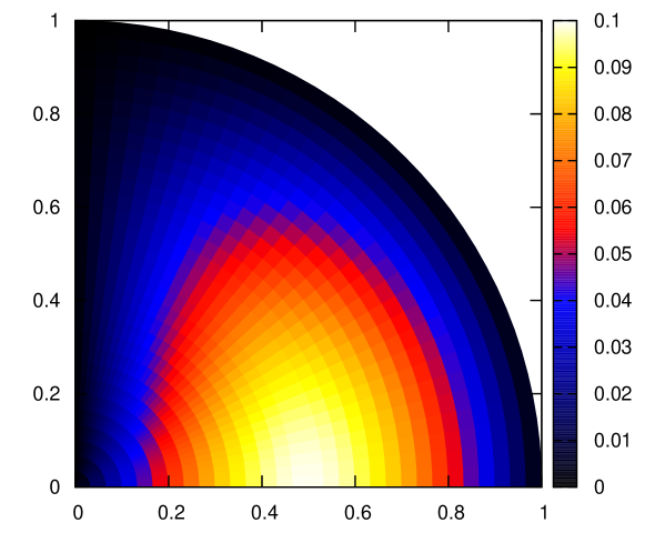
Figure 6: The toroidal field configuration of the background star. Note that the field vanishes on the pole and at the surface, reaching a maximum at a dimensionless radius $r/R\sim 0.5$ from the centre.

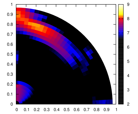
Figure 7: The magnitude of the perturbed magnetic field after the onset of instability. The most unstable perturbations are visible around the magnetic axis and in a region close to the stellar surface, where the background field is weak. The growth of the instability is shown by dividing the perturbed field through by an early-time perturbed field configuration.

One of the predictions made by Tayler (1973) is that an $m=1$ toroidal-field instability is likely to develop around the magnetic field’s symmetry axis (though this does not exclude the possibility of it growing elsewhere within the star too). From a global evolution, however, it is not straightforward to isolate the behaviour of the instability from stable perturbations. Plots of $|\delta{\bf B}|$ across the numerical domain can be dominated by the shape of an initially stable perturbation, whereas we are interested in where $|\delta{\bf B}|$ grows fastest after the onset of instability. To monitor the instability’s growth, we divide the value of $|\delta{\bf B}|$ at each point by its value at some early time. We find that these plots then have a generic structure similar to the one shown in figure 7: the perturbation grows fast around the axis, as expected, but also in a shell towards the stellar surface. Comparing this with the shape of the background field, shown in figure 7, we see that the instability grows fastest where the background field is weak. This resembles the situation for poloidal-field instabilities — these grow fastest around the region where the background field vanishes (Markey & Tayler, 1973).

\psfrag{growth}{$\zeta$/[s${}^{-1}$]}\psfrag{Bav}{$\bar{B}$/[$10^{16}$ G]}\psfrag{Om}{$\hat{\Omega}$}\psfrag{B3}{$\bar{B}=3.0\times 10^{16}$ G}\psfrag{B1.5}{$\bar{B}=1.5\times 10^{16}$ G}\includegraphics[width=433.62pt]{growth_norot_rot.eps}

Figure 8: Left: the instability growth rate (in seconds^-1) plotted against field strength $\bar{B}$ for a series of nonrotating stars; we see that the dependence is linear for these field strengths. Right: The effect of rotation on the growth rate, for two values of $\bar{B}$. At $\hat{\Omega}=0$ the weaker-field growth rate is half that of the stronger one; when $\hat{\Omega}>0$ it reduces to approximately a quarter that of the stronger one.

We now wish to quantify how the growth rate $\zeta$ of the Tayler instability depends on field strength $\bar{B}$ and rotation rate $\Omega$. For early times, the behaviour of the magnetic perturbations will be a sum of various stable oscillatory modes and the unstable perturbation $\propto\exp(kt)$ ($k\in\mathbb{R}_{+}$) which concerns us; eventually, the amplitude of this unstable perturbation will become dominant (see figure 5) and hence we may extract its growth rate. We define

$$\zeta=\frac{1}{\Delta t}\ \Delta\left({\ln\left({\frac{\delta M}{M_{0}}}\right)}\right)$$ (18)

as a measure of growth, where $M_{0}$ is the magnetic energy of the background. In figure 8 we use this to investigate how toroidal-field instabilities depend on the field strength and rotation rate of the star. In the left-hand plot we show that $\zeta$ depends linearly on $\bar{B}$, whilst in the right-hand plot we investigate the dependence of $\zeta$ on rotation rate $\Omega$, for $1.5$ and $3.0\times 10^{16}$ G fields. At $\Omega=0$ $\zeta$ is half the value for the weaker field (since it is linear in $\bar{B}$), but for $\Omega>0$ the weaker field’s growth rate $\zeta_{1.5}$ is about a quarter that of the stronger one $\zeta_{3}$. This is consistent with the suggestion of Tayler (1973) that $\zeta$ should depend on the ratio of magnetic to rotational energy $M/T$: if $\zeta_{3}\sim M_{3}/T$ and $\zeta_{1.5}\sim M_{1.5}/T$, then $\zeta_{3}/\zeta_{1.5}\sim M_{3}/M_{1.5}\sim B_{3}^{2}/B_{1.5}^{2}=3^{2}/1.5^{2}=4$. We note that rotation reduces the instability, but does not appear to stabilise the field entirely; this is in agreement with the work of Pitts & Tayler (1985) and Kitchatinov & Rüdiger (2008).

We conclude with a brief mention of $m\geq 2$ instabilities. In Lander, Jones & Passamonti (2010) we employed an artificial resistivity term to damp out long-timescale instabilities in our evolutions. We returned to study those instabilities for this work, but found that their growth rates did not converge satisfactorily with resolution; hence, we can not convincingly claim to have seen evidence of higher-$m$ toroidal-field instabilities. This is not surprising, though, as these are weaker than the $m=1$ instability.

5 Tayler-instability effects in magnetars

Magnetars in the SGR class are notable for their great variability in luminosity. In addition to their quiescent emission of $\sim 10^{35}$ erg s^-1, they undergo periods of short bursts at luminosities of up to $\sim 10^{42}$ erg s^-1. Rarely, they suffer enormously energetic ‘giant flares’, during which their luminosity exceeds $\sim 10^{44}$ erg s^-1 ($\sim 10^{47}$ erg s^-1, in the case of SGR 1806-20) (Mereghetti, 2008). It is not clear what provides the trigger mechanism for, in particular, these giant flares; a number of internal and magnetospheric processes have been suggested (see, for example, Thompson & Duncan (1996) or Gill & Heyl (2010) and references therein).

The Tayler instability is one possible candidate for an internal SGR-flare trigger, as discussed briefly in Thompson & Duncan (1996); see also the related work on magnetic-field reconfiguration by Ioka (2001). Suppose a magnetar field is dominantly toroidal — such a configuration could come from, for example, differential rotation winding up a mixed field at the star’s birth. The small poloidal component will help to suppress the toroidal-field instability discussed in this paper, but nonetheless the field could be on the verge of an unstable regime. One could imagine some dissipative process weakening the poloidal component, or some relatively minor field rearrangement occurring near the symmetry axis of the field. The resulting field configuration could then be susceptible to the Tayler instability, causing an exponentially-growing perturbation in the magnetic energy which manifests itself as a giant flare at the star’s surface.

If this mechanism were the trigger for SGR flares, what could we learn about magnetar fields? Let us return to the left-hand plot in figure 8, where we plot the instability growth rate $\zeta$ against averaged-field strength $\bar{B}$ for nonrotating stars (this is appropriate for magnetars, whose rotational frequencies are close to zero). Now consider a growth timescale $\tau_{grow}=1/\zeta$ (in seconds) for the instability. Our results give an empirical relation

$$\tau_{grow}=1.9\left({\frac{\bar{B}}{10^{16}\ \mathrm{G}}}\right)^{-1}\ \mathrm{ms}$$ (19)

— i.e, $\tau_{grow}=0.019$ seconds for a $\bar{B}=10^{15}$ G field and $\tau_{grow}=1.9$ ms for a $10^{16}$ G field. This latter value is comparable with upper limits on the initial rise times for the three observed giant flares: 1.3 ms (SGR 1806-20), 1.6 ms (SGR 1900+14) and 2 ms (SGR 0526-66) (Tanaka et al., 2007). If we associate these rise times with $\tau_{grow}$ then we obtain values for the averaged-field strength of $0.95,1.2$ and $1.5\times 10^{16}$ G for SGRs 0526-66, 1900+14 and 1806-20 respectively. These values seem reasonable in the context of recent estimates (Stella et al., 2005; Kaminker et al., 2007) for magnetar internal field strengths.

Finally, if the trigger mechanism for giant flares resembles a large $m=1$ perturbation of the magnetic field, as we suggest here, it would induce a corresponding disturbance in the stellar density distribution. The $l\geq 2$ harmonics in this disturbance will produce gravitational radiation — making SGR giant flares a suitable, if rare, target for gravitational-wave burst searches from advanced LIGO. We are, however, unable to estimate the amplitude of these bursts, since nonlinear effects (not included in our work) would become important after the initial rise time.

6 Discussion

In this paper we have shown that the unstable nature of purely toroidal magnetic fields, well-known from local analyses about the magnetic axis, may also be seen from a global evolution of linear perturbations. In particular, a generic configuration that emerges when studying axisymmetric Newtonian MHD — where $B_{\phi}$ is proportional to $\rho r\sin\theta$ — proves to be unstable to $m=1$ perturbations. The instability is reduced, but not eliminated, by rotation; this agrees with the suggestion of Pitts & Tayler (1985) and the studies by Kiuchi, Shibata & Yoshida (2008) and Kitchatinov & Rüdiger (2008). Braithwaite (2006) found rotation could entirely stabilise certain toroidal-field configurations. We have quantified the dependence of the instability growth rate on field strength and rotation rate.

The Tayler instability rules out generic purely-toroidal configurations as candidates for physical stellar fields in strict equilibrium (at least in barotropic-fluid stars; see Reisenegger (2009) for arguments that it may be a poor assumption to regard stars as barotropic). The instability could however be of astrophysical interest: if a stellar magnetic field is dominantly toroidal it is likely it will be close to unstable, with relatively minor disturbances able to trigger the instability. We have discussed the possibility of such a mechanism causing the giant flares of SGRs, and motivation for gravitational-wave burst searches coincident with these giant flares.

Although the Tayler instability may be relevant in explaining SGR flares, we are many steps away from a credible study of magnetic-field stability in neutron stars. Natural topics for further studies would be the stability of purely poloidal fields and mixed-field configurations, which we intend to consider in future work. Further into the future, one might hope to consider the effect of superconductivity and/or an elastic crust, and so build up a more realistic picture of neutron star stability.

References

- Andersson & Kokkotas (2001) Andersson N., Kokkotas K.D., 2001, International Journal of Modern Physics D, 10, 381
- Arfken & Weber (2001) Arfken G.B., Weber H.J., 2001, Mathematical Methods for Physicists, Harcourt Academic Press
- Braithwaite (2006) Braithwaite J., 2006, A&A, 453, 687
- Christensen-Dalsgaard & Gough (2001) Christensen-Dalsgaard J., Gough D.O., 2001, MNRAS, 326, 1115
- Dedner et al. (2002) Dedner A., Kemm F., Kröner D., Munz C.-D., Schnitzer T., Wesenberg M., 2002, J. Comp. Phys., 175, 645
- Dib, Kaspi & Gavriil (2007) Dib R., Kaspi V.M., Gavriil F.P., 2007, ApJ, 673, 1044
- Duncan & Thompson (1992) Duncan R.C., Thompson C., 1992, ApJ, 392, L9
- Gill & Heyl (2010) Gill R., Heyl J.S., 2010, arXiv:1002.3662
- Glampedakis & Andersson (2007) Glampedakis K., Andersson N., 2007, MNRAS, 377, 630
- Goossens & Tayler (1980) Goossens M., Tayler R.J., 1980, MNRAS, 193, 833
- Ioka (2001) Ioka K., 2001, MNRAS, 327, 639
- Kaminker et al. (2007) Kaminker A.D., Yakovlev D.G., Potekhin A.Y., Shibazaki N., Shternin P.S., Gnedin O.Y., 2007, Ap&SS, 308, 423
- Kitchatinov & Rüdiger (2008) Kitchatinov L.L., Rüdiger G., 2008, A&A, 478, 1
- Kiuchi, Shibata & Yoshida (2008) Kiuchi K., Shibata M., Yoshida S., 2008, PRD, 78, 024029
- Lander & Jones (2009) Lander S.K., Jones D.I., 2009, MNRAS, 395, 2162
- Lander, Jones & Passamonti (2010) Lander S.K., Jones D.I., Passamonti A., 2010, MNRAS, 405, 318
- Lockitch & Friedman (1999) Lockitch K.H., Friedman J.L., 1999, ApJ, 521, 764
- Markey & Tayler (1973) Markey P., Tayler R.J., 1973, MNRAS, 163, 77
- Mereghetti (2008) Mereghetti S., 2008, A&A Rev., 15, 225
- Miralles, Pons & Urpin (2002) Miralles J.A., Pons J.A., Urpin V.A., 2002, ApJ, 574, 356
- Pitts & Tayler (1985) Pitts E., Tayler R.J., 1985, MNRAS, 216, 139
- Price & Monaghan (2005) Price D.J., Monaghan J.J., 2005, MNRAS, 364, 384
- Reisenegger (2009) Reisenegger A., 2009, A&A, 499, 557
- Rezzolla, Lamb & Shapiro (2000) Rezzolla L., Lamb F.K., Shapiro S.L., 2000, ApJ, 531, L139
- Roxburgh (1963) Roxburgh I.W., 1963, MNRAS, 126, 67
- Roxburgh & Durney (1967) Roxburgh I.W., Durney B.R., 1967, MNRAS, 135, 329
- Stella et al. (2005) Stella L., Dall’Osso S., Israel G.L., Vecchio A., 2005, ApJ, 634, L165
- Tanaka et al. (2007) Tanaka Y.T., Terasawa T., Kawai N., Yoshida A., Yoshikawa I., Saito Y., Takashima T., Mukai T., 2007, ApJ, 665, L55
- Tayler (1973) Tayler R.J., 1973, MNRAS, 161, 365
- Thompson & Duncan (1996) Thompson C., Duncan R.C., 1996, ApJ, 473, 322
- Yoshida & Lee (2000) Yoshida S., Lee U., 2000, ApJ, 529, 997