Delay-Optimal User Scheduling and Inter-Cell Interference Management in Cellular Network via Distributive Stochastic Learning

Abstract

In this paper, we propose a distributive queue-aware intra-cell user scheduling and inter-cell interference (ICI) management control design for a delay-optimal celluar downlink system with $M$ base stations (BSs), and $K$ users in each cell. Each BS has $K$ downlink queues for $K$ users respectively with heterogeneous arrivals and delay requirements. The ICI management control is adaptive to joint queue state information (QSI) over a slow time scale, while the user scheduling control is adaptive to both the joint QSI and the joint channel state information (CSI) over a faster time scale. We show that the problem can be modeled as an infinite horizon average cost Partially Observed Markov Decision Problem (POMDP), which is NP-hard in general. By exploiting the special structure of the problem, we shall derive an equivalent Bellman equation to solve the POMDP problem. To address the distributive requirement and the issue of dimensionality and computation complexity, we derive a distributive online stochastic learning algorithm, which only requires local QSI and local CSI at each of the $M$ BSs. We show that the proposed learning algorithm converges almost-surely (with probability 1) and has significant gain compared with various baselines. The proposed solution only has linear complexity order $O(MK)$.

I Introduction

It is well-known that cellular systems are interference limited and there are a lot of works to handle the inter-cell interference (ICI) in cellular systems. Specifically, the optimal binary power control (BPC) for the sum rate maximization has been studied in [1]. They showed that BPC could provide reasonable performance compared with the multi-level power control in the multi-link system. In [2], the authors studied a joint adaptive multi-pattern reuse and intra-cell user scheduling scheme, to maximize the long-term network-wide utility. The ICI management runs at a slower scale than the user selection strategy to reduce the communication overhead. In [3] and the reference therein, cooperation or coordination is also shown to be a useful tool to manage ICI and improve the performance of the celluar network.

However, all of these works have assumed that there are infinite backlogs at the transmitter, and the control policy is only a function of channel state information (CSI). In practice, applications are delay sensitive, and it is critical to optimize the delay performance in the cellular network. A systematic approach in dealing with delay-optimal resource control in general delay regime is via Markov Decision Process (MDP) technique. In [4, 5], the authors applied it to obtain the delay-optimal cross-layer control policy for broadcast channel and point-to-point link respectively. However, there are very limited works that studied the delay optimal control problem in the cellular network. Most existing works simply proposed heuristic control schemes with partial consideration of the queuing delay[6]. As we shall illustrate, there are various technical challenges involved regarding delay-optimal cellular network.

• Curse of Dimensionality: Although MDP technique is the systematic approach to solve the delay-optimal control problem, a primal difficulty is the curse of dimensionality[7]. For example, a huge state space (exponential in the number of users and number of cells) will be involved in the MDP and brute force value or policy iterations cannot lead to any implementable solution [8, 9]. Furthermore, brute force solutions require explicit knowledge of transition probability of system states, which is difficult to obtain in the complex systems.

• Complexity of the Interference Management: Jointly optimal ICI management and user scheduling requires heavy computation overhead even for the throughput optimization problem [2]. Although grouping clusters of cells [1] and considering only neighboring BSs [10] were proposed to reduce the complexity, complex operations on a slot by slot basis are still required, which is not suitable for the practical implementation.

• Decentralized Solution: For delay-optimal multi-cell control, the entire system state is characterized by the global CSI (CSI from any BS to any MS) and the global QSI (queue length of all users). Such system state information are distributed locally at each BS and centralized solution (which requires global knowledge of the CSI and QSI) will induce substantial signaling overhead between the BSs and the Base Station Controller (BSC).

In this paper, we consider the delay-optimal inter-cell ICI management control and intra-cell user scheduling for the cellular system. For implementation consideration, the ICI management control is computed at the BSC at a longer time scale and it is adaptive to the QSI only. On the other hand, the intra-cell user scheduling control is computed distributively at the BS at a smaller time scale and hence, it is adaptive to both the CSI and QSI. Due to the two time-scale control structure, the delay optimal control is formulated as an infinite-horizon average cost Partially Observed Markov Decision Process (POMDP). Exploiting the special structure, we propose an equivalent Bellman Equation to solve the POMDP. Based on the equivalent Bellman equation, we propose a distributive online learning algorithm to estimate a per-user value function as well as a per-user $\mathbb{Q}$-factor. Only the local CSI and QSI information is required in the learning process at each BS. We also establish the technical proof for the almost-sure convergence of the proposed distributive learning algorithm. The proposed algorithm is quite different from the iterative update algorithm for solving the deterministic NUM [12], where the CSI is always assumed to be quasi-static during the iterative updates. However, the delay-optimal problem we considered is stochastic in nature, and during the iterative updates, the system state will not be quasi-static anymore. In addition, the proposed learning algorithm is also quite different from conventional stochastic learning[11, 13]. For instance, conventional stochastic learning requires centralized update and global system state knowledge and the convergence proof follows from standard contraction mapping arguments[7]. However, due to the distributive learning requirement and simultaneous learning of the per-user value function and $\mathbb{Q}$-factor, it is not trivial to establish the contraction mapping property and the associated convergence proof. We also illustrate the performance gain of the proposed solution against various baselines via numerical simulations. Furthermore, the solution has linear complexity order $O(MK)$ and it is quite suitable for the practical implementation.

II System Model

In this section, we shall elaborate the system model, as well as the control policies. We consider the downlink of a wireless celluar network consisting of $M$ BSs, and there are $K$ mobile users in each cell served by one BS. Specifically, let $\mathcal{M}=\{1,...,M\}$ and $\mathcal{K}_{m}=\{1,...,K\}$ denote the set of BSs and the set of users served by the BS $m$ respectively. $k\in\mathcal{K}_{m}$ denotes the $k$-th user served by BS $m$. The time dimension is partitioned into scheduling slots (every slot lasts for $\tau$ seconds). The system model is illustrated in Fig.1.

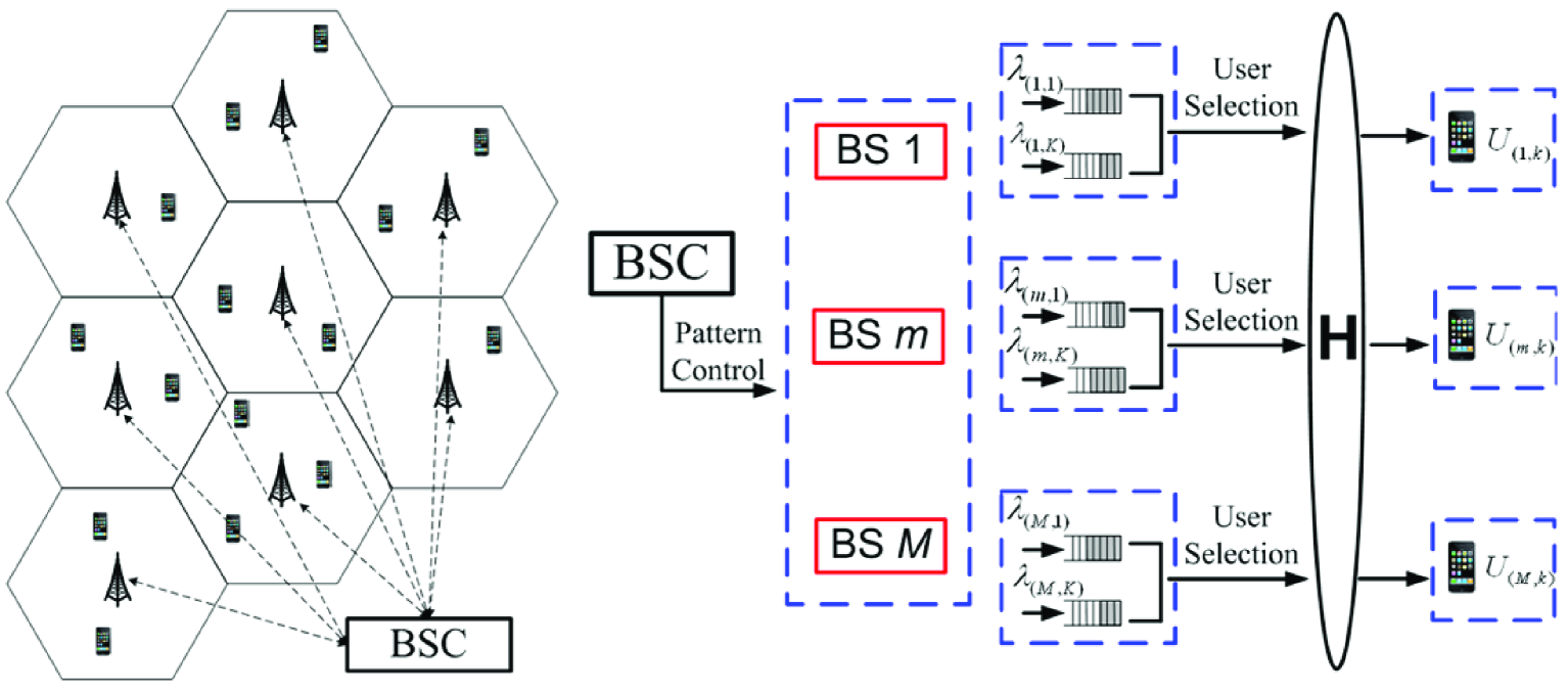
Figure 1: Physical layer and queueing model of celluar network.

II-A Source Model

In each BS, there are $K$ independent application streams dedicated to the $K$ users respectively. Let $\mathbf{A}(t)=\{\mathbf{A}_{m}(t)\}_{m=1}^{M}$ and $\mathbf{A}_{m}(t)=\{A_{(m,k)}(t)\}_{k=1}^{K}$, where $A_{(m,k)}(t)$ represents the new arrivals (number of bits) for the user $k\in\mathcal{K}_{m}$ at the end of the slot $t$.

Assumption 1 (Assumption on Source Model)

We assume that the arrival process $A_{(m,k)}(t)$ is i.i.d over the scheduling slot $t$ according to a general distribution $\Pr\{A_{(m,k)}\}$ with average arrival rate $\lambda_{(m,k)}=\mathbb{E}[A_{(m,k)}]$, and the arrival processes for all the users are independent with each other, i.e., $\Pr\{A_{(m,k)}A_{(n,l)}\}=\Pr\{A_{(m,k)}\}\Pr\{A_{(n,l)}\}$ if $m\neq n$ or $k\neq l$.   ∎

Let $\mathbf{Q}(t)=\{\mathbf{Q}_{m}(t)\}_{m=1}^{M}\in\mathcal{Q}$ denote the global QSI in the system, where $\mathcal{Q}$ is the state space for the global QSI. $\mathbf{Q}_{m}(t)=\{Q_{(m,k)}(t)\}_{k=1}^{K}$ denotes the QSI in the BS $m$, where $Q_{(m,k)}(t)$ represents the number of bits for user $k\in\mathcal{K}_{m}$ at the beginning of the slot $t$, and $N_{Q}$ denotes the maximal buffer size (bits). When the buffer is full, i.e, $Q_{(m,k)}=N_{Q}$, new bits arrivals will be dropped. The cardinality of the global QSI is $I_{Q}=(1+N_{Q})^{MK}$.

II-B Channel Model and Physical Layer Model

Let $H_{(m,k)}^{n}(t)$ and $L_{(m,k)}^{n}$ denote the small scale channel fading gain and the path loss from the $n$-th BS to the user $k\in\mathcal{K}_{m}$ respectively, and $\mathbf{H}_{(m,k)}(t)=\{H_{(m,k)}^{n}(t)\}_{n=1}^{M}$ is the local CSI states for user $k$. $\mathbf{H}_{m}(t)=\{\mathbf{H}_{(m,k)}(t)\}_{k=1}^{K}$ denotes the local CSI states for BS $m$, and the global CSI is denoted as $\mathbf{H}(t)=\{\mathbf{H}_{m}(t)\}_{m=1}^{M}\in\mathcal{H}$, where $\mathcal{H}$ is the state space for the global CSI.

Assumption 2 (Assumption on Channel Model)

We assume that the global $\mathbf{H}$ is quasi-static in each slot. Furthermore, $H_{(m,k)}^{n}(t)$ is i.i.d over the scheduling slot $t$ according to a general distribution $\Pr\{H_{(m,k)}^{n}\}$ and the small scale channel fading gains for all users are independent with each other. The path loss $L_{(m,k)}^{n}$ remains constant for the duration of the communication session.   ∎

The cellular system shares a single common channel with bandwidth $W$Hz (all the BSs use the same channel). At the beginning of each slot, the BS is either turned on (with transmit power $P^{m}_{\max}$) or off (with transmit power 0), according to a ICI management control policy, which is defined later. At each slot, a BS can select only one user for its data transmission. Specifically, let $\mathbf{p}=\{p_{m}\}_{m=1}^{M}\in\mathcal{P}$ denotes an ICI management control pattern, where $p_{m}=1$ denotes BS $m$ is active, $p_{m}=0$ otherwise, and $\mathcal{P}$ denotes the set of all possible control patterns. Furthermore, let $\mathcal{M}_{\mathbf{p}}\in\mathcal{M}$ be the set of BSs activated by the pattern $\mathbf{p}$ and $\mathcal{P}_{m}\in\mathcal{P}$ be the set of patterns that activate the BS $m$. The signal received by the user $k\in\mathcal{K}_{m}$ at slot $t$, when pattern $\mathbf{p}\in\mathcal{P}_{m}$ is selected, is given by

$$\begin{array}[]{l}y_{(m,k)}[t]=\sqrt{H^{m}_{(m,k)}L^{m}_{(m,k)}}x_{m}[t]+\\ \quad\quad\quad\quad\sum\nolimits_{n\neq m,n\in\mathcal{M}_{\mathbf{p}}}\sqrt{H^{n}_{(m,k)}L_{(m,k)}^{n}}x_{n}[t]+z[t]\end{array}$$ (1)

where $x_{m}[t]$ is the transmit signal from the $m$-th BS to the $k$-th user at slot $t$, and $\{z[t]\}_{t=1}^{\infty}$ is the i.i.d $\mathcal{N}(0,N_{0})$ noise. The achievable data rate of user $k$ can be expressed by

$$\begin{array}[]{l}R_{(m,k)}=\\ \left\{\begin{array}[]{ll}W\log_{2}\left(1+\frac{\xi P^{m}_{\max}H^{m}_{(m,k)}L_{(m,k)}^{m}}{I_{(m,k)}+N_{0}W}\right)s_{(m,k)}&\text{if $\mathbf{p}\in\mathcal{P}_{m}$}\\ 0&\text{otherwise}\end{array}\right.\end{array}$$ (2)

where $I_{(m,k)}=\sum\limits_{n\neq m,n\in\mathcal{M}_{\mathbf{p}}}P^{n}_{\max}H^{n}_{(m,k)}L_{(m,k)}^{n}$, $s_{(m,k)}\in\{0,1\}$ is an indicator variable with $s_{(m,k)}=1$ when the user $k$ is scheduled. $\xi\in(0,1]$ is a constant can be used to model both the coded and uncoded systems[5].

II-C ICI Management and User Scheduling Control Policy

At the beginning of the slot, the BSC will decide which BSs are allowed to transmit according to a stationary ICI management control policy defined below.

Definition 1 (Stationary ICI Management Control Policy)

A stationary ICI management control policy $\Omega_{\mathbf{p}}:\mathcal{Q}\rightarrow\mathcal{P}$ is defined as the mapping from current global QSI to an ICI management pattern $\Omega_{\mathbf{p}}(\mathbf{Q})=\mathbf{p}$.   ∎

Let $\boldsymbol{\chi}(t)=\{\mathbf{H}(t),\mathbf{Q}(t)\}$ to be the global system state at the beginning of slot $t$. The active user at each cell is selected according to a user scheduling policy defined below.

Definition 2 (Stationary User Scheduling Policy)

A stationary user scheduling policy $\Omega_{\mathbf{s}}:\{\mathcal{Q},\mathcal{H}\}\rightarrow\mathcal{S}$ is defined as the mapping from current global system state $\boldsymbol{\chi}$ to current user scheduling action $\Omega_{\mathbf{s}}(\boldsymbol{\chi})=\mathbf{s}\in\mathcal{S}$. The scheduling action $\mathbf{s}$ is a set of all the users' scheduling indicator variable, i.e., $\mathbf{s}=\{s_{(m,k)},\forall k\in\mathcal{K}_{m},\forall m\}$. It represents which users are scheduled and which users are not in any given slot. $\mathcal{S}$ is the set of all user scheduling actions.   ∎

For notation convenience, let $\Omega=\{\Omega_{\mathbf{p}},\Omega_{\mathbf{s}}\}$ to be the joint control policy, and $\Omega(\boldsymbol{\chi})=\{\mathbf{p},\mathbf{s}\}$ be the control action under state $\boldsymbol{\chi}$.

III Problem Formulation

In this section, we will first elaborate the dynamics of system state under a control policy $\Omega$. Based on that, we shall formally formulate the delay-optimal control problem.

III-A Dynamics of System State

Given the new arrival $A_{(m,k)}(t)$ at the end of the slot $t$, the current system state $\boldsymbol{\chi}(t)$ and the control action $\Omega(\boldsymbol{\chi}(t))$, The queue evolution for user $k\in\mathcal{K}_{m}$ is given by:

$$Q_{(m,k)}(t+1)=\big{[}\big{(}Q_{(m,k)}(t)-U_{(m,k)}(t)\big{)}^{+}+A_{(m,k)}(t)\big{]}_{\bigwedge N_{Q}}$$ (3)

where $U_{(m,k)}(t)=\lfloor R_{(m,k)}(\boldsymbol{\chi}(t),\Omega(\boldsymbol{\chi}(t)))\tau\rfloor$ is the number of bits delivered to user $k$ at slot $t$, and $R_{(m,k)}(\boldsymbol{\chi}(t),\Omega(\boldsymbol{\chi}(t)))$, given by (2), is the achievable data rate under the control action $\Omega(\boldsymbol{\chi}(t))$. $\lfloor x\rfloor$ denotes the floor of $x$, $(x)^{+}=\max(x,0)$, and $(x)_{\bigwedge N_{Q}}=\min(x,N_{Q})$. Let $\mathbf{U}(t)=\{\mathbf{U}_{m}(t)\}_{m=1}^{M}$, and $\mathbf{U}_{m}(t)=\{U_{(m,k)}(t)\}_{k=1}^{K}$, $U_{(m,k)}(t)=R_{(m,k)}(\boldsymbol{\chi}(t),\Omega(\boldsymbol{\chi}(t)))\tau$ for the user $k\in\mathcal{K}_{m}$, and $\mathbf{\hat{Q}}(t+1)=\big{[}\big{(}\mathbf{Q}(t)-\mathbf{U}(t)\big{)}^{+}+\mathbf{A}(t)\big{]}_{\bigwedge N_{Q}}$. Therefore, given a control policy $\Omega$, the random process $\{\mathbf{H}(t),\mathbf{Q}(t)\}$ is a controlled Markov chain with transition probability

$$\begin{array}[]{l}\Pr\{\boldsymbol{\chi}(t+1)|\boldsymbol{\chi}(t),\Omega(\boldsymbol{\chi}(t))\}=\\ \left\{\begin{array}[]{ll}\Pr\{\mathbf{H}(t+1)\}\Pr\{\mathbf{A}(t)\}&\text{if $\mathbf{Q}(t+1)=\mathbf{\hat{Q}}(t+1)$}\\ 0&\text{otherwise}\end{array}\right.\end{array}$$ (4)

III-B Delay Optimal Control Problem Formulation

Given a stationary control policy $\Omega$, the average cost of the user $k\in\mathcal{K}_{m}$ is given by:

$$\overline{T}_{(m,k)}(\Omega)=\lim\sup_{T\rightarrow\infty}\frac{1}{T}\sum\nolimits_{t=1}^{T}\mathbb{E}[f(Q_{(m,k)}(t))]$$ (5)

where $f(Q_{(m,k)})$ is a monotonic increasing cost function of $Q_{(m,k)}$. For example, when $f(Q_{(m,k)})=Q_{(m,k)}/\lambda_{(m,k)}$, using Little's Law [4, 14], $\overline{T}_{(m,k)}(\Omega)$ is an approximation of the average delay of user $k$. When $f(Q_{(m,k)})=1_{\{Q_{(m,k)}\geq N_{Q}\}}$ and $A_{(m,k)}$ follows the bernoulli process, $\overline{T}_{(m,k)}(\Omega)$ is the bit dropping probability (conditioned on bit arrival). Note that, the $MK$ queues in the celluar system are coupled together via the control policy $\Omega$. In this paper, we seek to find an optimal stationary control policy $\Omega$ to minimize the average cost in (5). Specifically, we have:

Problem 1 (Delay Optimal Multi-cell Control Problem)

For some positive constants $\boldsymbol{\beta}=\{\beta_{(m,k)},,\forall k\in\mathcal{K}_{m},\forall m\}$, finding a stationary control policy $\Omega$ that minimizes:

$$\min_{\Omega}J_{\beta}^{\Omega} = \sum\nolimits_{m,k}\beta_{(m,k)}\overline{T}_{(m,k)}(\Omega)$$

$$= \lim\sup_{T\rightarrow\infty}\frac{1}{T}\sum\nolimits_{t=1}^{T}\mathbb{E}^{\Omega}[g(\boldsymbol{\chi}(t),\Omega(\boldsymbol{\chi}(t)))]$$

where $g(\boldsymbol{\chi}(t),\Omega(\boldsymbol{\chi}(t))=\sum_{m,k}\beta_{(m,k)}f(Q_{(m,k)})$ is the per-slot cost, and $\mathbb{E}^{\Omega}$ denotes the expectation w.r.t. the induced measure (induced by the control policy $\Omega$ and the transition kernel in (4)). The positive constants $\boldsymbol{\beta}$ indicate the relative importance of the users and for a given $\boldsymbol{\beta}$, the solution to (1) corresponds to a Pareto optimal point of the multi-objective optimization problem given by $\min_{\Omega}\overline{T}_{(m,k)}(\Omega),\forall m,k$. Moreover, a control policy $\Omega^{*}$ is called Pareto optimal if for any control policy $\Omega^{\prime}\neq\Omega^{*}$ such that $\overline{T}_{(m,k)}(\Omega^{\prime})\leq\overline{T}_{(m,k)}(\Omega^{*}),\forall m,k$, it implies that $\overline{T}_{(m,k)}(\Omega^{\prime})=\overline{T}_{(m,k)}(\Omega^{*}),\forall m,k$. In other words, we cannot reduce $\overline{T}_{(m,k1)}$ without increasing other component (say $\overline{T}_{(m,k2)}$) at Pareto optimal control $\Omega^{*}$[15].

IV General Solution to the Delay Optimal Problem

In this section, we will show that the delay optimal problem 1 can be modeled as an infinite horizon average cost POMDP, which is a very difficult problem. By exploiting the special structure, we shall derive an equivalent Bellman equation to solve the POMDP problem.

IV-A Preliminary on MDP and POMDP

An infinite horizon average cost MDP can be characterized by a tuple of four objects: $\{\mathbb{S},\mathbb{A},\Pr\{s^{\prime}|s,a\},g(s,a)\}$, where $\mathbb{S}$ is a finite set of states and $\mathbb{A}$ is the action space. $\Pr\{s^{\prime}|s,a\}$ is the transition probability from state $s$ to $s^{\prime}$, given that the action $a\in\mathbb{A}$ is taken. $g(s,a)$ is the per-slot cost function. The objective is to find the optimal policy $\mathbf{a}=\{a(s)\}$ so as to minimize the average per-slot cost $\theta$ as:

$$\theta=\min_{\mathbf{a}}\lim_{T\rightarrow\infty}\sup\frac{1}{T}\sum\nolimits_{t=1}^{T}\mathbb{E}^{\mathbf{a}}[g(s(t),a(s(t)))]$$ (7)

If the policy space consists of unichain policies and the associated induced Markov chain is irreducible, it is well known that there exist a unique $\theta$ for each starting state[11, 7]. Furthermore, the optimal control policy $\mathbf{a}$ can be obtained by the following Bellman equation.

$$V(s)+\theta=\min_{a(s)}\left\{g(s,a(s))+\sum\nolimits_{s^{\prime}}\Pr\{s^{\prime}|s,a(s)\}V(s^{\prime}))\right\}$$ (8)

where $V(s)$ is called the value function. General offline solutions, value or policy iteration, can be used to find the value function $V(s)$ iteratively, as well as the optimal policy[7].

POMDP is an extension of MDP when the control agent does not have direct observation of the entire system state (and hence it is called ``partially observed MDP''). Specifically, an infinite horizon average cost POMDP can be characterized by a tuple [16, 17]: $\{\mathbb{S},\mathbb{A},\Pr\{s^{\prime}|s,a\},g(s,a),\mathbb{O},O(z,s,a)\}$, where $\{\mathbb{S},\mathbb{A},P(s^{\prime}|s,a),g(s,a)\}$ characterize a MDP and $\mathbb{O}$ is a finite set of observations. $O(z,s,a)$ is the observation function, which gives the probability (or stochastic relationship) between the partial observation $z$, the actual system state $s$ and the control action $a$. Specifically, $O(z,s,a)$ is the probability of getting a partial observation ``$z$'' given that the current system state is $s$ and the action $a$ was taken in the previous slot. A PODMP is a MDP where current system state and the actions are based on the observation $z$. The objective is to find the optimal policy $\mathbf{a}=\{a(z)\}$ so as to minimize the average per-slot cost $\theta$ in (7). However, in general, it is a NP-hard problem and there are various approximation solutions proposed based on the special structure of the studied problems[18].

IV-B Equivalent Bellman Equation and Optimal Control Policy

In this subsection, we shall first illustrate that the optimization problem 1 is an infinite horizon average cost POMDP. We shall then exploit some special problem structure to simplify the complexity and derive an equivalent Bellman equation to solve the problem. For instance, in the delay optimal problem 1, the ICI management control policy $\Omega_{\mathbf{p}}$ is adaptive to the QSI $\mathbf{Q}$, while the user scheduling policy $\Omega_{\mathbf{s}}$ is adaptive to the complete system state $\{\mathbf{Q},\mathbf{H}\}$. Therefore, the optimal control policy $\Omega^{*}$ cannot be obtained by solving a standard Bellman equation from conventional MDP. In fact, problem 1 is a POMDP with the following specification.

• State Space: The system state is the global QSI and CSI $\boldsymbol{\chi}=\{\mathbf{Q},\mathbf{H}\}\in\{\mathcal{Q},\mathcal{H}\}$.

• Action Space: The action is ICI management pattern and user scheduling $\{\mathbf{p},\mathbf{s}\}\in\{\mathcal{P},\mathcal{S}\}$.

• Transition Kernel: The transition probability $\Pr\{\boldsymbol{\chi}^{\prime}|\boldsymbol{\chi},\mathbf{p},\mathbf{s}\}$ is given in (4).

• Per-Slot Cost Function: The per-slot cost function is $g(\boldsymbol{\chi},\mathbf{p},\mathbf{s})=\sum_{m,k}\beta_{(m,k)}f(Q_{(m,k)})$.

• Observation: The observation for ICI management control policy is global QSI, i.e., $z_{\mathbf{p}}=\mathbf{Q}$, while the observation for User scheduling policy is the complete system state, i.e., $z_{\mathbf{s}}=\boldsymbol{\chi}$.

• Observation Function: The observation function for ICI management control policy is $O_{\mathbf{p}}(z_{\mathbf{p}},\boldsymbol{\chi},\mathbf{p},\mathbf{s})=1$, if $z_{\mathbf{p}}=\mathbf{Q}$, otherwise 0. Furthermore the observation function for user scheduling policy is $O_{\mathbf{s}}(z_{\mathbf{s}},\boldsymbol{\chi},\mathbf{p},\mathbf{s})=1$, if $z_{\mathbf{s}}=\boldsymbol{\chi}$, otherwise 0.

While POMDP is a very difficult problem in general, we shall utilize the notion of action partitioning in our problem to substantially simplify the problem. We first define partitioned actions below.

Definition 3 (Partitioned Actions)

Given a control policy $\Omega$, we define $\Omega(\mathbf{Q})=\{(\mathbf{p},\mathbf{s})=\Omega(\boldsymbol{\chi}):\boldsymbol{\chi}=(\mathbf{Q},\mathbf{H})\forall\mathbf{H}\in\mathcal{H}\}$ as the collection of actions under a given $\mathbf{Q}$ for all possible $\mathbf{H}\in\mathcal{H}$. The complete policy $\Omega$ is therefore equal to the union of all partitioned actions, i.e., $\Omega=\bigcup_{\mathbf{Q}}\Omega(\mathbf{Q})$.   ∎

Based on the action partitioning, we can transform the POMDP problem into a regular infinite-horizon average cost MDP. Furthermore, the optimal control policy $\Omega^{*}$ can be obtained by solving an equivalent Bellman equation which is summarized in the theorem below.

Theorem 1 (Equivalent Bellman Equation)

The optimal control policy $\Omega^{*}=(\Omega_{\mathbf{p}}^{*},\Omega_{\mathbf{s}}^{*})$ in problem 1 can be obtained by solving the equivalent Bellman equation given by:

$$V(\mathbf{Q})+\theta=\min_{\Omega(\mathbf{Q})}\Big{[}\hat{g}(\mathbf{Q},\Omega(\mathbf{Q}))+\sum\limits_{\mathbf{Q}^{\prime}}\Pr\{\mathbf{Q}^{\prime}|\mathbf{Q},\Omega(\mathbf{Q})\}V(\mathbf{Q}^{\prime})\Big{]}$$ (9)

where $\hat{g}(\mathbf{Q},\Omega(\mathbf{Q}))=\sum_{m,k}\beta_{(m,k)}f(Q_{(m,k)})$ is the per-slot cost function, and the transition kernel is given by $\Pr\{\mathbf{Q}^{\prime}|\mathbf{Q},\Omega(\mathbf{Q})\}=\mathbb{E}_{\mathbf{H}}\left[\Pr\{\mathbf{Q}^{\prime}|\mathbf{Q},\mathbf{H},\Omega(\boldsymbol{\chi})\}\right]$, where $\Pr\{\mathbf{Q}^{\prime}|\mathbf{Q},\mathbf{H},\Omega(\boldsymbol{\chi})\}$ is given by

$$\begin{array}[]{l}\Pr\{\mathbf{Q}^{\prime}|\mathbf{Q},\mathbf{H},\Omega(\boldsymbol{\chi})\}=\\ \quad\quad\left\{\begin{array}[]{ll}\Pr\{\mathbf{A}\}&\text{if $\mathbf{Q}^{\prime}=\Big{[}\big{(}\mathbf{Q}-\mathbf{U}\big{)}^{+}+\mathbf{A}\Big{]}_{\bigwedge N_{Q}}$}\\ 0&\text{otherwise}\end{array}\right.\end{array}$$ (10)

where $\mathbf{U}=\{\mathbf{U}_{m}\}_{m=1}^{M}$, and $\mathbf{U}_{m}=\{U_{(m,k)}\}_{k=1}^{K}$, and $U_{(m,k)}=R_{(m,k)}(\boldsymbol{\chi},\Omega(\boldsymbol{\chi}))\tau$ for $k\in\mathcal{K}_{m}$. Suppose $\Omega^{*}(\mathbf{Q})=\{\mathbf{p}^{*}({\mathbf{Q}}),\bigcup_{\mathbf{H}}\mathbf{s}^{*}(\mathbf{Q},\mathbf{H})\}$ is a solution that solves the Bellman equation in (9), the optimal control policy for the original Problem 1 is given by: $\Omega_{\mathbf{p}}^{*}=\bigcup_{\mathbf{Q}}\{\mathbf{p}^{*}(\mathbf{Q})\}$ and $\Omega_{\mathbf{s}}^{*}=\bigcup_{\mathbf{Q},\mathbf{H}}\{\mathbf{s}^{*}(\mathbf{Q},\mathbf{H})\}$. The value function $V(\mathbf{Q})$ that solves (9) is a component-wise monotonic increasing function.   ∎

Proof:

Please refer to Appendix A. ∎

Note that solving (9) will obtain an ICI management policy $\Omega_{\mathbf{p}}^{*}$ that is a function of QSI $\mathbf{Q}$ and a user scheduling policy $\Omega_{\mathbf{s}}^{*}$ that is a function of the QSI and CSI $\{\mathbf{Q},\mathbf{H}\}$. We shall illustrate this with a simple example below.

Example 1

Suppose there are two BSs with equal transmitting power ($P^{m}_{\max}=P,\forall m$), and there are three ICI management control patterns in $\mathcal{P}$, given by $\mathbf{p}_{1}=\{p_{1}=1,p_{2}=0\}$ (BS 1 is active), $\mathbf{p}_{2}=\{p_{1}=0,p_{2}=1\}$ (BS 2 is active) and $\mathbf{p}_{3}=\{p_{1}=1,p_{2}=1\}$ (both BSs are active). Assume deterministic arrival where one bit will always arrive at each slot, i.e., $\Pr\{A_{(m,k)}=1\}=1$. The number of users served by each BS is $K=2$. The path loss $L_{(m,k)}^{n}=1$ for all $\{k,n,m\}$, and the small scale fading gain is chosen from two values $\{H_{g},H_{b}\}$ with equal probability. As a result, the global CSI state space is $\mathcal{H}=\{H_{g},H_{b}\}^{M^{2}K}$. Note that the cardinality of CSI state space $\mathcal{H}$ is $|\mathcal{H}|=2^{M^{2}K}=256$. Given a realization of the global QSI $\mathbf{Q}$, the partitioned actions (following Definition 3) is given by:

$$\Omega(\mathbf{Q})=\{\mathbf{p}(\mathbf{Q}),\mathbf{s}(\mathbf{Q},\mathbf{H}^{(1)}),\cdots,\mathbf{s}(\mathbf{Q},\mathbf{H}^{(256)})\}$$ (11)

Using Theorem 1, the optimal partitioned action $\Omega^{*}(\mathbf{Q})$ is given by solving the right hand side (RHS) of (9):

$$\begin{array}[]{l}\Omega^{*}(\mathbf{Q})=\operatorname*{\arg\min}\limits_{\{\mathbf{p}(\mathbf{Q}),\{\mathbf{s}(\mathbf{Q},\mathbf{H}^{(i)})\}_{i=1}^{256}\}}\sum_{\mathbf{Q}^{\prime}}\sum_{\mathbf{H}^{(i)}\in\mathcal{H}}\\ \quad\Big{[}\Pr\{\mathbf{H}^{(i)}\}\Pr\{\mathbf{Q}^{\prime}|\mathbf{Q},\mathbf{H}^{(i)},\mathbf{p}(\mathbf{Q}),\mathbf{s}(\mathbf{Q},\mathbf{H}^{(i)})\}V(\mathbf{Q}^{\prime})\Big{]}\end{array}$$ (12)

where

$$\begin{array}[]{l}\Pr\{\mathbf{Q}^{\prime}|\mathbf{Q},\mathbf{H}^{(i)},\mathbf{p}(\mathbf{Q}),\mathbf{s}(\mathbf{Q},\mathbf{H}^{(i)})\}=\\ \quad\quad\quad\quad\left\{\begin{array}[]{ll}1&\text{if }\mathbf{Q}^{\prime}=\Big{[}\big{(}\mathbf{Q}-\mathbf{U}\big{)}^{+}+\mathbf{1}\Big{]}_{\bigwedge N_{Q}}\\ 0&\text{otherwise}\end{array}\right.\end{array}$$ (13)

and $\mathbf{U}=\{U_{(1,1)},U_{(1,2)};U_{(2,1)},U_{(2,2)}\}$ is the number of departure bits. For a given ICI management control $\mathbf{p}(\mathbf{Q})=\mathbf{p}$, the optimal user scheduling policy $\{\mathbf{s}^{*}(\mathbf{Q},\mathbf{H}^{(i)})\}$ is

$$\begin{array}[]{l}\{\mathbf{s}^{*}(\mathbf{Q},\mathbf{H}^{(i)})\}=\operatorname*{\arg\min}\limits_{\{\mathbf{s}(\mathbf{Q},\mathbf{H}^{(i)})\}_{i=1}^{256}}\sum_{\mathbf{Q}^{\prime}}\sum_{\mathbf{H}^{(i)}\in\mathcal{H}}\\ \quad\Big{[}\Pr\{\mathbf{H}^{(i)}\}\Pr\{\mathbf{Q}^{\prime}|\mathbf{Q},\mathbf{H}^{(i)},\mathbf{p},\mathbf{s}(\mathbf{Q},\mathbf{H}^{(i)})\}V(\mathbf{Q}^{\prime})\Big{]}\end{array}$$ (14)

Observe that the RHS of (14) is a decoupled objective function w.r.t. the variables $\{\mathbf{s}(\mathbf{Q},\mathbf{H}^{(i)})\}_{i=1}^{256}$ and hence, applying standard decomposition theory,

$$\begin{array}[]{l}\mathbf{s}^{*}(\mathbf{Q},\mathbf{H}^{(i)})=\\ \quad\operatorname*{\arg\min}\limits_{\mathbf{s}(\mathbf{Q},\mathbf{H}^{(i)})}\sum\limits_{\mathbf{Q}^{\prime}}\Pr\{\mathbf{Q}^{\prime}|\mathbf{Q},\mathbf{H}^{(i)},\mathbf{p},\mathbf{s}(\mathbf{Q},\mathbf{H}^{(i)})\}V(\mathbf{Q}^{\prime})\end{array}$$ (15)

As a result, the optimal ICI management control policy $\mathbf{p}^{*}(\mathbf{Q})$ is given by:

$$\begin{array}[]{l}\mathbf{p}^{*}(\mathbf{Q})=\operatorname*{\arg\min}_{\mathbf{p}(\mathbf{Q})}\sum\nolimits_{\mathbf{Q}^{\prime}}\sum\nolimits_{\mathbf{H}^{(i)}\in\mathcal{H}}\\ \quad\Big{[}\Pr\{\mathbf{H}^{(i)}\}\Pr\{\mathbf{Q}^{\prime}|\mathbf{Q},\mathbf{H}^{(i)},\mathbf{p}(\mathbf{Q}),\mathbf{s}^{*}(\mathbf{Q},\mathbf{H}^{(i)})\}V(\mathbf{Q}^{\prime})\Big{]}\end{array}$$ (16)

where $\mathbf{s}^{*}(\mathbf{Q},\mathbf{H}^{(i)})$ given in (15) is the optimal user scheduling policy under the ICI management control policy $\mathbf{p}(\mathbf{Q})$. Using Theorem 1, the optimal ICI management control and user selection control of the original Problem 1 for a CSI realization $\mathbf{H}^{(i)}$ and QSI realization $\mathbf{Q}$ are given by $\mathbf{p}^{*}(\mathbf{Q})$ and $\mathbf{s}^{*}(\mathbf{Q},\mathbf{H}^{(i)})$ respectively.   ∎

V Distributive Value Function and $\mathbb{Q}$-factor Online Learning

The solution in Theorem 1 requires the knowledge of the value function $V(\mathbf{Q})$. However, obtaining the value function is not trivial as solving the Bellman equation (9) involves solving a very large system of the nonlinear fixed point equations (corresponding to each realization of $\mathbf{Q}$ in (9)). Brute-force solution of $V(\mathbf{Q})$ require huge complexity, centralized implementation and knowledge of global CSI and QSI at the BSC. This will also induce huge signaling overhead because the QSI of all the users are maintained locally at the $M$ BSs. In this section, we shall propose a decentralized solution via distributive stochastic learning following the structure as illustrated in Fig. 2. Moreover, we shall prove that the proposed distributive stochastic learning algorithm will converge almost-surely.

V-A Post-Decision State Framework

In this section, we first introduce the post-decision state also used framework, also used in [19] and the references therein, to lay ground for developing the online learning algorithm. The post-decision state is defined to be the virtual system state immediately after making an action but before the new bits arrive. For example, $\boldsymbol{\chi}=\{\mathbf{Q},\mathbf{H}\}$ is the state at the beginning of some time slot (also called the pre-decision state), and making an action $\Omega(\boldsymbol{\chi})=\{\mathbf{p},\mathbf{s}\}$, the post-decision state immediately after the action is $\widetilde{\boldsymbol{\chi}}=\{\widetilde{\mathbf{Q}},\mathbf{H}\}$, where the transition to $\widetilde{\mathbf{Q}}$ is given by $\widetilde{\mathbf{Q}}=\big{(}\mathbf{Q}-\mathbf{U}\big{)}^{+}$. If new arrivals $\mathbf{A}$ occur in the post-decision state, and the CSI changes to $\mathbf{H}^{\prime}$, then the system reaches the next actual state, i.e., pre-decision state, $\boldsymbol{\chi}^{\prime}=\{\big{[}\widetilde{\mathbf{Q}}+\mathbf{A}\big{]}_{\bigwedge N_{Q}},\mathbf{H}^{\prime}\}$.

Using the action partitioning and defining the value function $\widetilde{\mathbf{V}}$ on post-decision state $\widetilde{\mathbf{Q}}$ (where pre-decision state is $\{\mathbf{Q}=\big{[}\widetilde{\mathbf{Q}}+\mathbf{A}\big{]}_{\bigwedge N_{Q}},\mathbf{H}\}$), $\widetilde{\mathbf{V}}$ will satisfy the post-decision state Bellman equation[19]

$$\begin{array}[]{l}\widetilde{V}(\widetilde{\mathbf{Q}})+\theta=\sum_{\mathbf{A}}\Pr\{\mathbf{A}\}\bigg{\{}\min_{\Omega(\mathbf{Q})}\Big{[}\widetilde{g}(\mathbf{Q},\Omega(\mathbf{Q}))\\ \quad\quad\quad\quad+\sum\nolimits_{\widetilde{\mathbf{Q}}^{\prime}}\Pr\{\widetilde{\mathbf{Q}}^{\prime}|\mathbf{Q},\Omega(\mathbf{Q})\}\widetilde{V}(\widetilde{\mathbf{Q}}^{\prime})\Big{]}\bigg{\}}\end{array}$$ (17)

where $\widetilde{g}(\mathbf{Q},\Omega(\mathbf{Q}))=\sum_{m,k}\beta_{(m,k)}f(Q_{(m,k)})$, $\Pr\{\widetilde{\mathbf{Q}}^{\prime}|\mathbf{Q},\Omega(\mathbf{Q})\}=\mathbb{E}_{\mathbf{H}}[\Pr\{\widetilde{\mathbf{Q}}^{\prime}|\mathbf{Q},\mathbf{H},\Omega(\mathbf{Q})\}]$, and $\widetilde{\mathbf{Q}}^{\prime}$ is the next post-decision state transited from $\mathbf{Q}$. As Theorem 1, $\widetilde{V}(\widetilde{\mathbf{Q}})$ is also a component-wise monotonic increasing function. The optimal policy is obtained by solving the RHS of Bellman equation (17).

V-B Distributive User Scheduling Policy on the CSI Time Scale

To reduce the size of the state space and to decentralize the user scheduling, we approximate $\widetilde{V}(\widetilde{\mathbf{Q}})$ in (17) by the sum of per-user post-decision state value function $\widetilde{V}_{(m,k)}(\widetilde{Q}_{(m,k)})$, i.e.,

$$\widetilde{V}(\widetilde{\mathbf{Q}})\approx\sum\nolimits_{m,k}\widetilde{V}_{(m,k)}(\widetilde{Q}_{(m,k)})$$ (18)

where $\widetilde{V}_{(m,k)}(\widetilde{Q}_{(m,k)})$ is defined as the fixed point of the following per-user fixed point equation:

$$\begin{array}[]{l}\widetilde{V}_{(m,k)}(\widetilde{Q}_{(m,k)})+\widetilde{V}_{(m,k)}(\widetilde{Q}_{(m,k)}^{I})=\\ \sum\nolimits_{A_{(m,k)}}\Pr\{A_{(m,k)}\}\Big{[}\beta_{(m,k)}f(Q_{(m,k)})+\\ \sum\limits_{\widetilde{Q}_{(m,k)}^{\prime}}\Pr\{\widetilde{Q}_{(m,k)}^{\prime}|Q_{(m,k)},s_{(m,k)}=1,\widetilde{\mathbf{p}}_{m}^{I}\}\widetilde{V}_{(m,k)}(\widetilde{Q}_{(m,k)}^{\prime})\Big{]}\end{array}$$ (19)

where $Q_{(m,k)}=\widetilde{Q}_{(m,k)}+A_{(m,k)}$ is the pre-decision state, $s_{(m,k)}=1$ means that the user $k$ is scheduled to transmit at BS $m$, $\widetilde{Q}_{(m,k)}^{I}\in\{0,\cdots,N_{Q}\}$ is a reference state and $\widetilde{\mathbf{p}}_{m}^{I}\in\mathcal{P}_{m}$ is a reference ICI management pattern (with the BS $m$ active). The per-user value function $\widetilde{V}_{(m,k)}(\widetilde{Q}_{(m,k)})$ is obtained by the proposed distributive online learning algorithm (explained in section V-D). Note that the state space for the value function of $\widetilde{V}(\widetilde{\mathbf{Q}})$ is substantially reduced from $(N_{Q}+1)^{MK}$ (exponential growth w.r.t the number of all mobile users $MK$) to $MK(N_{Q}+1)$ (linear growth w.r.t the number of all mobile users).

Corollary 1 (Decentralized User Scheduling Actions)

Using the linear approximation in (18), the user scheduling action of BS $m\in\mathcal{M}_{\mathbf{p}}$ under any given ICI management pattern $\mathbf{p}$ (obtained by solving the RHS of Bellman equation (17)) is given by:

$$\mathbf{s}_{m}=\{s_{k^{*}}=1,s_{(m,k)}=0,\forall k\neq k^{*}\text{ and }k,k^{*}\in\mathcal{K}_{m}\}$$ (20)

where $k^{*}=\arg\max_{k\in\mathcal{K}_{m}}\widetilde{\delta}_{(m,k)}(Q_{(m,k)})$, and $\widetilde{\delta}_{(m,k)}(Q_{(m,k)})=\widetilde{V}_{(m,k)}(Q_{(m,k)})-\widetilde{V}_{(m,k)}((Q_{(m,k)}-U_{(m,k)})^{+})$. $U_{(m,k)}=\log_{2}\left(1+\frac{\xi\phi_{(m,k)}}{\varphi_{(m,k)}}\right)\tau$, where $\varphi_{(m,k)}=\sum\limits_{n\neq m,n\in\mathcal{M}_{\mathbf{p}}}P^{n}_{\max}H^{n}_{(m,k)}L_{(m,k)}^{n}+N_{0}W$ is the power sum of interference and noise, and $\phi_{(m,k)}=P^{m}_{\max}H^{m}_{(m,k)}L_{(m,k)}^{m}$ is the signal power.   ∎

Proof:

Please refer to Appendix B. ∎

Remark 1 (Structure of the User Scheduling Actions)

The user scheduling action in (20) is both function of local CSI and QSI. Specifically, the number of bits to be delivered $U_{(m,k)}$ is controlled by the local CSI $\mathbf{H}_{(m,k)}$, and local QSI $Q_{(m,k)}$ will determine $\widetilde{\delta}_{(m,k)}(Q_{(m,k)})$. Each user estimates $\varphi_{(m,k)}$ and $\phi_{(m,k)}$ in the preamble phase, and sends $U_{(m,k)}$ to the associated BS $m$ according to the process as indicated in Fig.2.   ∎

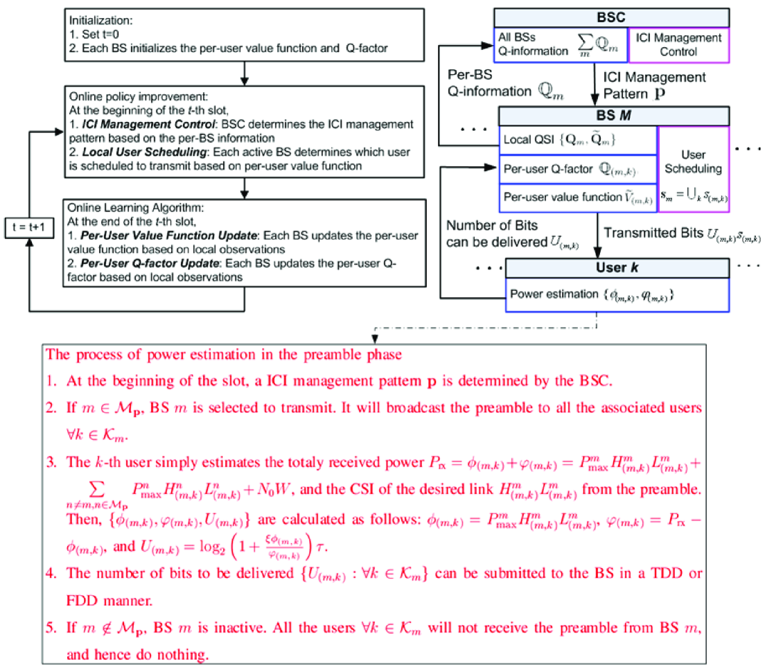
Figure 2: The system procedure for distributive per-user value function and per-user $\mathbb{Q}$-factor online learning algorithm.

V-C ICI Management Control Policy on the QSI Time Scale

To determine the ICI management control policy, we define the $\mathbb{Q}$-factor as follows [11]:

$$\begin{array}[]{l}\mathbb{Q}(\mathbf{Q},\mathbf{p})=\sum\nolimits_{m,k}\beta_{(m,k)}f(Q_{(m,k)})+\\ \quad\quad\quad\sum\nolimits_{\mathbf{Q}^{\prime}}\Pr\{\mathbf{Q}^{\prime}|\mathbf{Q},\mathbf{p}\}\min_{\mathbf{p}^{\prime}}\mathbb{Q}(\mathbf{Q}^{\prime},\mathbf{p}^{\prime})-\theta\end{array}$$ (21)

where $\Pr\{\mathbf{Q}^{\prime}|\mathbf{Q},\mathbf{p}\}$ is the transition probability from current QSI $\mathbf{Q}$ to $\mathbf{Q}^{\prime}$, given current action $\mathbf{p}$, and $\theta$ is a constant. Note that the $\mathbb{Q}$-factor $\mathbb{Q}(\mathbf{Q},\mathbf{p})$ represents the potential cost of applying a control action $\mathbf{p}$ at the current QSI $\mathbf{Q}$ and applying the action $\arg\min_{\mathbf{p}^{\prime}}\mathbb{Q}(\mathbf{Q}^{\prime},\mathbf{p}^{\prime})$ for any system state $\mathbf{Q}^{\prime}$ in the future. Similar to (18), we approximate the $\mathbb{Q}$-factor in (21) with a sum of per-user $\mathbb{Q}$-factor, i.e,

$$\mathbb{Q}(\mathbf{Q},\mathbf{p})\approx\sum\nolimits_{m,k}\mathbb{Q}_{(m,k)}(Q_{(m,k)},\mathbf{p})$$ (22)

where $\mathbb{Q}_{(m,k)}$ is defined as the fixed point of the following per-user fixed point equation:

$$\begin{array}[]{l}\mathbb{Q}_{(m,k)}(Q_{(m,k)},\mathbf{p})=\\ \beta_{(m,k)}f(Q_{(m,k)})-\mathbb{Q}_{(m,k)}(Q_{(m,k)}^{I},\mathbf{p}^{I}_{m})+\sum\limits_{Q_{(m,k)}^{\prime}}\\ \Big{[}\Pr\{Q_{(m,k)}^{\prime}|Q_{(m,k)},s_{(m,k)}=1,\mathbf{p}\}\min\limits_{\mathbf{p}^{\prime}}\mathbb{Q}_{(m,k)}(Q_{(m,k)}^{\prime},\mathbf{p}^{\prime})\Big{]}\end{array}$$ (23)

where $\Pr\{Q_{(m,k)}^{\prime}|Q_{(m,k)},s_{(m,k)}=1,\mathbf{p}\}=\mathbb{E}_{\mathbf{H}_{(m,k)}}[\Pr\{Q_{(m,k)}^{\prime}|Q_{(m,k)},s_{(m,k)}=1,\mathbf{H}_{(m,k)},\mathbf{p}\}]$. $Q_{(m,k)}^{I}\in\{0,\cdots,N_{Q}\}$ is a reference state and $\mathbf{p}^{I}_{m}\in\mathcal{P}$ is a reference ICI management control pattern. The per-user $\mathbb{Q}$-factor $\mathbb{Q}_{(m,k)}$ is obtained by the proposed distributive online learning algorithm (explained in section V-D). The BSC collects the per-BS $\mathbb{Q}$-information $\mathbb{Q}_{m}^{t}(\mathbf{p})=\sum_{(m,k)}\mathbb{Q}_{(m,k)}^{t}(Q_{(m,k)}^{t},\mathbf{p})$ at the beginning of slot $t$, and the ICI management control policy is given by:

$$\mathbf{p}^{t}=\operatorname*{\arg\min}\nolimits_{\mathbf{p}}\sum\nolimits_{m}\mathbb{Q}_{m}^{t}(\mathbf{p})$$ (24)

In order to reduce the communication overhead between the $M$ BSs and the BSC, we could further partition the local QSI space into $N$ regions ($\mathcal{Q}_{m}=\bigcup_{n=1}^{N}\mathcal{R}_{n}$) as illustrated in Fig. 3. At the beginning of the $t$-th slot, the $m$-th BS will update the BSC of the per-BS $\mathbb{Q}$-information if its QSI state belongs to a new region. Hence, the per-BS $\mathbb{Q}$-information at the BSC is updated according to the following dynamics:

$$\begin{array}[]{l}\mathbb{Q}_{m}^{t}(\mathbf{p})=\\ \left\{\begin{array}[]{ll}\sum\limits_{m,k}\mathbb{Q}_{(m,k)}^{t}(Q_{(m,k)}^{t},\mathbf{p})&\text{if $\mathbf{Q}_{m}^{t}\in\mathcal{R}_{n},\mathbf{Q}_{m}^{t-1}\not\in\mathcal{R}_{n}$}\\ \mathbb{Q}_{m}^{t-1}(\mathbf{p})&\text{otherwise}\end{array}\right.\end{array}$$ (25)

Remark 2 (Communication Overhead)

The communication overhead between the $M$ BS and the BSC is reduced from $O((N_{Q}+1)^{MK}+(N_{H})^{M^{2}K})$ (exponential growth w.r.t the number of users $K$) to $O(M(\alpha)^{|\mathcal{P}|})$ for some constant $\alpha$ (O(1) w.r.t. $K$), where $N_{H}$ is the cardinality of the CSI state space for one link.   ∎

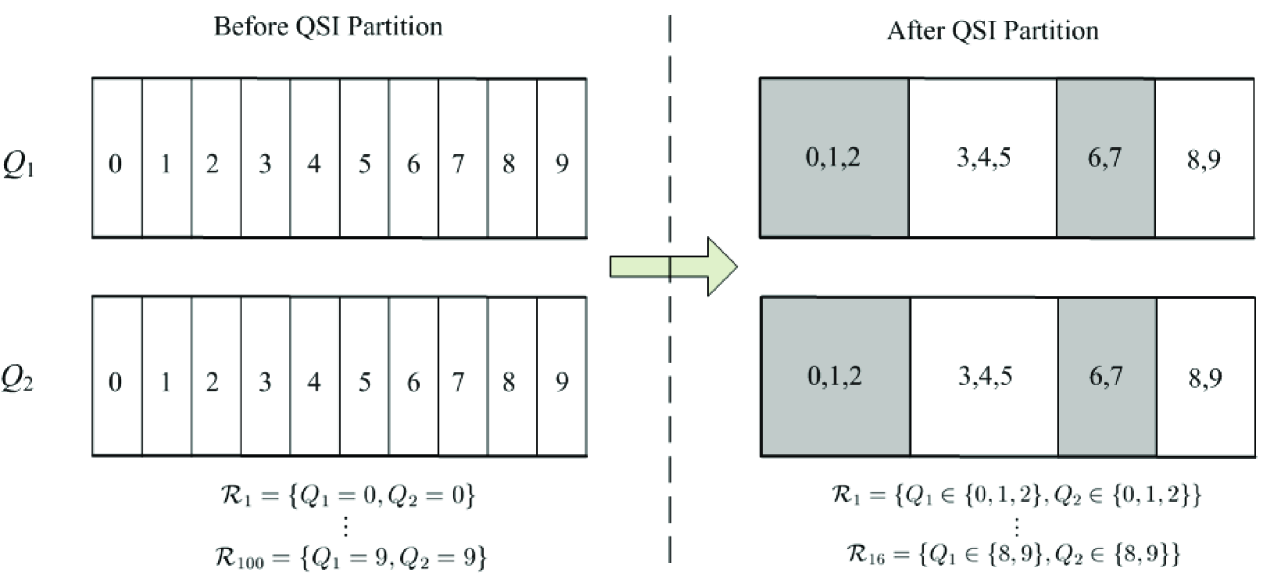
Figure 3: Illustration of one possible way of local QSI partition. There are $K=2$ users with buffer size $N_{Q}=9$, where each user's QSI is partitioned into 4 regions, given by $\big{\{}\{0,1,2\};\{3,4,5\};\{6,7\};\{8,9\}\big{\}}$. Note that the number of local QSI regions for one BS is largely reduced from $(N_{Q}+1)^{K}=100$ $\big{(}\mathcal{R}_{1}=\{Q_{1}=0,Q_{2}=0\},\cdots,\mathcal{R}_{100}=\{Q_{1}=9,Q_{2}=9\}\big{)}$ to $4^{K}=16$ $\big{(}\mathcal{R}_{1}=\{Q_{1}\in\{0,1,2\},Q_{2}\in\{0,1,2\}\},\cdots,\mathcal{R}_{16}=\{Q_{1}\in\{8,9\},Q_{2}\in\{8,9\}\}\big{)}$ after partition.

V-D Online Per-User Value Function and Per-User $\mathbb{Q}$-factor Learning Algorithm

The system procedure for distributive online learning is given below:

• Initialization: Each BS initiates the per-user value function and $\mathbb{Q}$-factor for its $K$ users, denoted as $\{\widetilde{V}_{(m,k)}^{0}\}$ and $\{\mathbb{Q}_{(m,k)}^{0}\}$, where $\widetilde{V}_{(m,k)}^{0}(Q^{\prime}_{(m,k)})>\widetilde{V}_{(m,k)}^{0}(Q_{(m,k)}),\forall Q^{\prime}_{(m,k)}>Q_{(m,k)}$.

• ICI Management Control: At the beginning of the $t$-th slot, the BSC updates the $\mathbb{Q}$-information $\mathbb{Q}_{m}^{t}(\mathbf{p})$ as (25) and determines the ICI management pattern as (24).

• User Scheduling: If $m\in\mathcal{M}_{\mathbf{p}^{t}}$, BS $m$ is selected to transmit. The user scheduling policy is determined according to (20).

• Local Per-user Value Function and Per-user $\mathbb{Q}$-factor Update: Based on the current observations, each of the $M$ BSs updates the per-user value function $\widetilde{V}_{(m,k)}$ and the per-user $\mathbb{Q}$-factor $\mathbb{Q}_{(m,k)}$ according to Algorithm 1.

Fig. 2 illustrates the above procedure by a flowchart. The algorithm for the per-user value function and per-user $\mathbb{Q}$-factor update is given below:

Algorithm 1 (Online Learning Algorithm)

Let $\widetilde{\mathbf{Q}}_{m}$ and $\mathbf{Q}_{m}$ be the current observation of post-decision and pre-decision states respectively, $\mathbf{A}_{m}$ be the current observation of new arrival, $\{\mathbf{H}_{(m,k)}\}_{k=1}^{K}$ be the current observation of the local CSI, and $\mathbf{p}$ is the realization of the ICI management control pattern. The online learning algorithm for user $k\in\mathcal{K}_{m}$ is given by

$$\begin{array}[]{l}\widetilde{V}_{(m,k)}^{t+1}(\widetilde{Q}_{(m,k)})=\\ \left\{\begin{array}[]{ll}\widetilde{V}_{(m,k)}^{t}(\widetilde{Q}_{(m,k)})+\gamma(t)\Bigl{[}\beta_{(m,k)}f(\widetilde{Q}_{(m,k)}+&\\ A_{(m,k)})+\widetilde{V}_{(m,k)}^{t}(\widetilde{Q}_{(m,k)}+A_{(m,k)}-U_{(m,k)})&\text{if }\mathbf{p}=\widetilde{\mathbf{p}}_{m}^{I}\\ \quad\quad-\widetilde{V}_{(m,k)}^{t}(\widetilde{Q}_{(m,k)}^{I})-\widetilde{V}_{(m,k)}^{t}(\widetilde{Q}_{(m,k)})\Bigr{]}&\\ \widetilde{V}_{(m,k)}^{t}(\widetilde{Q}_{(m,k)})&\text{otherwise}\end{array}\right.\end{array}$$ (26)

$$\begin{array}[]{l}\mathbb{Q}_{(m,k)}^{t+1}(Q_{(m,k)},\mathbf{p})=\mathbb{Q}_{(m,k)}^{t}(Q_{(m,k)},\mathbf{p})+\gamma(t)\Bigl{[}\beta_{(m,k)}\\ \cdot f(Q_{(m,k)})-\mathbb{Q}_{(m,k)}^{t}(Q_{(m,k)}^{I},\mathbf{p}_{m}^{I})-\mathbb{Q}_{(m,k)}^{t}(Q_{(m,k)},\mathbf{p})\\ +\min_{\mathbf{p}^{\prime}}\mathbb{Q}_{(m,k)}^{t}(Q_{(m,k)}-U_{(m,k)}+A_{(m,k)},\mathbf{p}^{\prime})\Bigr{]}\end{array}$$ (27)

where $U_{(m,k)}$ is the number of bits to be delivered for user $k$ (given in Corollary 1 and depends indirectly on the local CSI observations $\mathbf{H}_{(m,k)}$), $\{\widetilde{Q}_{(m,k)}^{I},\widetilde{\mathbf{p}}_{m}^{I}\}$ and $\{Q_{(m,k)}^{I},\mathbf{p}_{m}^{I}\}$ are the reference state and reference ICI management pattern for the value function $\widetilde{V}_{(m,k)}$ in (19) and $\mathbb{Q}$-factor $\mathbb{Q}_{(m,k)}$ in (23) respectively. $\gamma(n)$ is diminishing positive step size sequence satisfying $\sum_{n}\gamma(n)=\infty,\sum_{n}\gamma^{2}(n)<\infty$.   ∎

Remark 3 (Complexity of the Learning Algorithm)

The proposed learning scheme only requires the observations of the local QSI $\widetilde{\mathbf{Q}}_{m}$ and $\mathbf{Q}_{m}$. Furthermore, each users only need to feedback $U_{(m,k)}$ instead of the local CSI $\mathbf{H}_{m}$, which is of similar feedback loading compared with HSDPA systems.   ∎

V-E Convergence Analysis

In this section we will establish the convergence proof of the proposed per-user learning algorithm 1. We first define a mapping on the post-decision state $\widetilde{Q}_{(m,k)}$ as

$$\begin{array}[]{l}T_{(m,k)}(\widetilde{\mathbf{V}}_{(m,k)},\widetilde{Q}_{(m,k)})=\widetilde{g}_{(m,k)}(\widetilde{Q}_{(m,k)})+\\ \sum\limits_{\widetilde{Q}_{(m,k)}^{\prime}}\Pr\{\widetilde{Q}_{(m,k)}^{\prime}|\widetilde{Q}_{(m,k)},s_{(m,k)}=1,\widetilde{\mathbf{p}}_{m}^{I}\}\widetilde{V}_{(m,k)}(\widetilde{Q}_{(m,k)}^{\prime})\end{array}$$ (28)

where $Q_{(m,k)}=\widetilde{Q}_{(m,k)}+A_{(m,k)}$ is the pre-decision state, $\widetilde{g}_{(m,k)}(\widetilde{Q}_{(m,k)})=\mathbb{E}_{A_{(m,k)}}\big{[}\beta_{(m,k)}f(\widetilde{Q}_{(m,k)}+A_{(m,k)})\big{]}$, and $\Pr\{\widetilde{Q}_{(m,k)}^{\prime}|\widetilde{Q}_{(m,k)},s_{(m,k)}=1,\widetilde{\mathbf{p}}_{m}^{I}\}=\mathbb{E}_{\mathbf{H}_{(m,k)},A_{(m,k)}}[\Pr\{\widetilde{Q}_{(m,k)}^{\prime}|Q_{(m,k)},\mathbf{H}_{(m,k)},s_{(m,k)}=1,\widetilde{\mathbf{p}}_{m}^{I}\}]$. The vector form of the mapping is given by:

$$\mathbf{T}_{(m,k)}(\widetilde{\mathbf{V}}_{(m,k)})=\widetilde{\mathbf{g}}_{(m,k)}+\mathbf{P}_{(m,k)}\widetilde{\mathbf{V}}_{m}$$ (29)

where $\mathbf{P}_{(m,k)}$ is $(N_{Q}+1)\times(N_{Q}+1)$ transition matrix for the post-decision state queue of the user $k$. and $\widetilde{\mathbf{V}}_{(m,k)}$ are $(N_{Q}+1)\times 1$ vectors. Specifically, we have the following lemma for the per-user value function learning in (26).

Lemma 1 (Convergence of Per-User Value Function)

The update of the per-user value function $\widetilde{\mathbf{V}}_{(m,k)}^{t}$ will converge almost-surely in the proposed learning algorithm 1, i.e., $\lim_{t\rightarrow\infty}\widetilde{\mathbf{V}}_{(m,k)}^{t}=\widetilde{\mathbf{V}}_{(m,k)}^{\infty},\forall k,m$, and $\widetilde{V}_{(m,k)}^{\infty}(\widetilde{Q}_{(m,k)})$ is a monotonic increasing function satisfying:

$$\widetilde{\mathbf{V}}_{(m,k)}^{\infty}+\widetilde{V}_{(m,k)}^{\infty}(\widetilde{Q}_{(m,k)}^{I})\mathbf{e}=\mathbf{T}_{(m,k)}(\widetilde{\mathbf{V}}_{(m,k)}^{\infty})$$ (30)

Proof:

Please refer to Appendix C. ∎

Note that (30) is equivalent to the per-user fixed point equation in (19). This result illustrates that the proposed online distributive learning in (26) can converge to the target per-user fixed point solution in (19). We define a mapping for the per-user $\mathbb{Q}$-factor $\mathbb{Q}_{(m,k)}$ as

$$\begin{array}[]{l}T_{(m,k)}^{\mathbb{Q}}(\mathbb{Q}_{(m,k)},Q_{(m,k)},\mathbf{p})=\beta_{(m,k)}f(Q_{(m,k)})+\sum\limits_{Q_{(m,k)}^{\prime}}\\ \Big{[}\Pr\{Q_{(m,k)}^{\prime}|Q_{(m,k)},s_{(m,k)}=1,\mathbf{p}\}\min\limits_{\mathbf{p}^{\prime}}\mathbb{Q}_{(m,k)}(Q_{(m,k)}^{\prime},\mathbf{p}^{\prime})\Big{]}\end{array}$$ (31)

Specifically, we have following lemma for the $\mathbb{Q}$-factor online learning in (27).

Lemma 2 (Convergence of the Per-User $\mathbb{Q}$-factor)

The update of per-user $\mathbb{Q}$-factor $\mathbb{Q}_{(m,k)}$ will converge almost-surely in the proposed learning algorithm 1, i.e., $\lim_{t\rightarrow\infty}\mathbb{Q}_{(m,k)}^{t}=\mathbb{Q}_{(m,k)}^{\infty},\forall k,m$, where the steady state $\mathbb{Q}$-factor $\{\mathbb{Q}_{(m,k)}^{\infty}\}$ satisfy:

$$\begin{array}[]{l}\mathbb{Q}_{(m,k)}^{\infty}(Q_{(m,k)},\mathbf{p})=\\ \quad\quad T_{(m,k)}^{\mathbb{Q}}(\mathbb{Q}_{(m,k)}^{\infty},Q_{(m,k)},\mathbf{p})-\mathbb{Q}_{(m,k)}^{\infty}(Q_{(m,k)}^{I},\mathbf{p}^{I}_{m})\end{array}$$ (32)

Proof:

Please refer to Appendix D. ∎

Note that (32) is equivalent to the per-user fixed point equation for $\mathbb{Q}_{(m,k)}$ in (23). This result illustrates that the proposed online distributive learning in (27) can converge to the target per user fixed point solution in (23).

Lemma 1 and 2 only established the convergence of the proposed online learning algorithm. Strictly speaking, the converged result is not optimal due to the linear approximation of the value function $\widetilde{V}(\widetilde{\mathbf{Q}})$ and the $\mathbb{Q}$-factor $\mathbb{Q}(\mathbf{Q},\mathbf{p})$ in (18) and (22) respectively. The linear approximation is needed for distributive implementation. As illustrated in Fig. 4, the proposed distributive solution has close-to-optimal performance compared with brute-force centralized solution of the Bellman equation in (9).

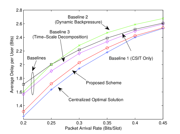
Figure 4: Average delay per user versus per user loading $\lambda_{(m,k)}$ in the Example 1 with the source arrival model is given by $\Pr\{A_{(m,k)}=1\}=\lambda_{(m,k)}$ and $\Pr\{A_{(m,k)}=0\}=1-\lambda_{(m,k)}$ for all $m,k$, and the buffer size $N_{Q}=3$. Centralized optimal solution refers to the brute-force centralized solution of the Bellman equation in (9). Baseline 1 refers to the CSIT only scheme, where the user scheduling are adaptive to the CSIT only. Baseline 2 refers to the Dynamic Backpressure scheme [20]. Baseline 3 refers to the time-scale decomposition scheme proposed in [2].

VI Simulation and Discussion

In this section, we shall compare the proposed distributive queue-aware intra-cell user scheduling and ICI management control scheme with three baselines. Baseline 1 refers to the CSIT only scheme, where the user scheduling are adaptive to the CSIT only so as to optimize the achievable data rate. Baseline 2 refers to a throughput optimal policy (in stability sense) for the user scheduling, namely the Dynamic Backpressure scheme [20]. In both baseline 1 and 2, the traditional frequency reuse scheme (frequency reuse factor equals 3) is used for inter-cell interference management. Baseline 3 refers to the time-scale decomposition scheme proposed in [2], where the sets of possible ICI management patterns $\mathcal{P}$ is the same as the proposed scheme. In the simulation, we consider a two-tier celluar network composed of 19 BSs as in [2], each has a coverage of 500m. Channel models are implemented according to the Urban Macrocell Model in 3GPP and Jakes' Rayleigh fading model. Specifically, the path loss model is given by $PL=34.5+35\log_{10}(r)$, where $r$ (in m) is the distance from the transmitter to the receiver. The total BW is 10MHz. We consider Poisson packet arrival with average arrival rate $\mathbb{E}[A_{(m,k)}]=\lambda_{(m,k)}$ (packets/slot) and exponentially distributed random packet size $\overline{N}_{(m,k)}$ with $\mathbb{E}[\overline{N}_{(m,k)}]=5$Mbits. The scheduling slot duration $\tau$ is 5ms. The maximum buffer size $N_{Q}$ is 9 (in packets), where each user's QSI is partitioned into 4 regions, given by $\big{\{}\{0,1,2\};\{3,4,5\};\{6,7\};\{8,9\}\big{\}}$. The cost function is given by $f(Q_{(m,k)})=\frac{Q_{(m,k)}}{\lambda_{(m,k)}}$ for all the users in the simulations.

VI-A Performance w.r.t. Transmit Power

Fig.5 and Fig.6 illustrate the performance of average delay and packet dropping probability (conditioned on packet arrival) per user versus transmit power $P_{\max}^{m}$ respectively. The number of users per BS $K=3$, and the average arrival rate $\lambda_{(m,k)}=1$. Note that the average delay and packet dropping probability of all the schemes decreases as the transmit power increases, and there is significant performance gain of the proposed scheme compared to all baselines. This gain is contributed by the QSI-aware user scheduling as well as ICI management control.

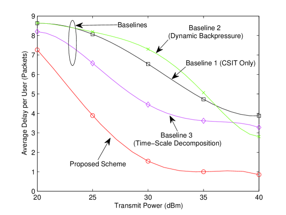
Figure 5: Average delay per user versus transmit power $P_{\max}^{m}$. The number of users per BS is $K=3$. The average arrival rate $\lambda_{(m,k)}=1$ (packets/slot). The maximum buffer size $N_{Q}$ is 9, where each user's QSI is partitioned into 4 regions, given by $\big{\{}\{0,1,2\};\{3,4,5\};\{6,7\};\{8,9\}\big{\}}$.

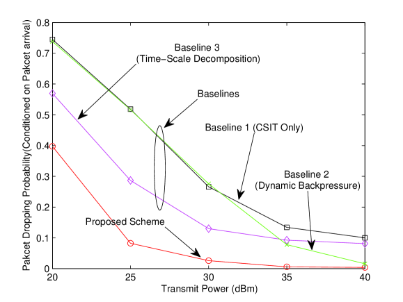
Figure 6: Packet dropping probability (conditioned on packet arrival) per user versus transmit power $P_{\max}^{m}$. The number of users per BS is $K=3$. The average arrival rate $\lambda_{(m,k)}=1$ (packets/slot). The maximum buffer size $N_{Q}$ is 9, where each user's QSI is partitioned into 4 regions, given by $\big{\{}\{0,1,2\};\{3,4,5\};\{6,7\};\{8,9\}\big{\}}$.

VI-B Performance w.r.t. Loading

Fig.7 illustrates the average delay versus per user loading (average arrival rate $\lambda_{(m,k)}$) at transmit power of $P_{\max}^{m}=30$dBm and the number of users per BS $K=3$. It can also be observed that the proposed scheme achieved significant gain over all the baselines across a wide range of input loading.

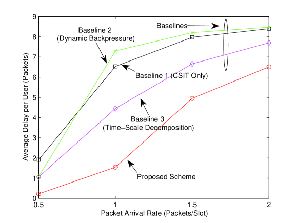
Figure 7: Average delay per user versus per user loading $\lambda_{(m,k)}$. The transmit power $P_{\max}^{m}=30$dBm. The number of users per BS is $K=3$. The maximum buffer size $N_{Q}$ is 9, where each user's QSI is partitioned into 4 regions, given by $\big{\{}\{0,1,2\};\{3,4,5\};\{6,7\};\{8,9\}\big{\}}$.

VI-C Cumulative Distribution Function (CDF) of the Queue Length

Fig.8 illustrates the Cumulative Distribution Function (CDF) of the queue length per user with transmit power $P_{\max}^{m}=25$dBm. The number of users per BS is $K=3$ and the average arrival rate $\lambda_{(m,k)}=1$. It can be also be verified that the proposed scheme achieves not only a smaller average delay but also a smaller delay percentile compared with the other baselines.

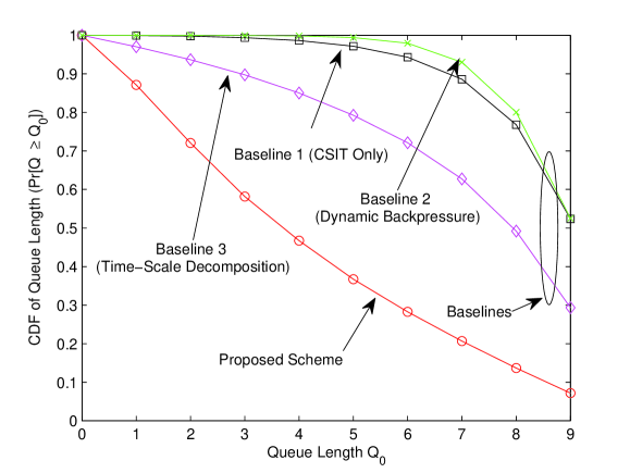
Figure 8: Cumulative Distribution Function (CDF) of the queue length per user with transmit power $P_{\max}^{m}=25$dBm. The number of users per BS is $K=3$. The average arrival rate $\lambda_{(m,k)}=1$. The maximum buffer size $N_{Q}$ is 9, where each user's QSI is partitioned into 4 regions, given by $\big{\{}\{0,1,2\};\{3,4,5\};\{6,7\};\{8,9\}\big{\}}$.

VI-D Convergence Performance

Fig.9 illustrates the average delay per user versus the scheduling slot index with transmit power $P_{\max}^{m}=35$dBm. The number of users per BS is $K=3$ and the average arrival rate $\lambda_{(m,k)}=1.5$. It can be observed that the convergence rate of the online algorithm is quite fast. For example, the delay performance of the proposed scheme already out-performs all the baselines at the $400$-th slot. Furthermore, the delay performance at $400$-th slot is already quite close to the converged average delay. Finally, unlike the conventional iterative NUM approach where the iterations are done offline within the coherence time of the CSI, the proposed iterative algorithm is updated over the same time scale of the CSI and QSI updates. Moreover, the iterative algorithm is online, meaning that useful payload are transmitted during the iterations.

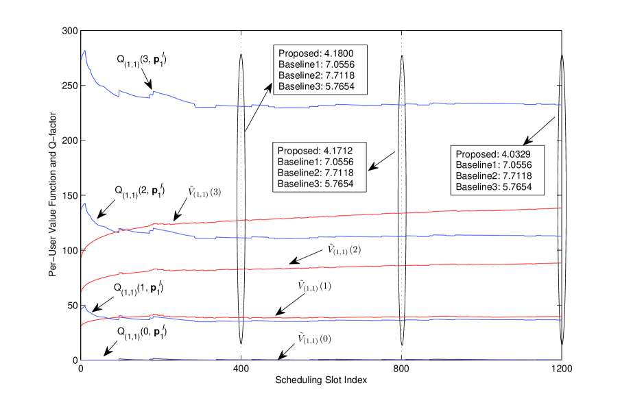
Figure 9: Convergence property of the proposed distributive stochastic learning algorithm via stochastic learning. The transmit power $P_{\max}^{m}=35$dBm. The number of users per BS is $K=3$. The average arrival rate $\lambda_{(m,k)}=1.5$. The maximum buffer size $N_{Q}$ is 9, where each user's QSI is partitioned into 4 regions, given by $\big{\{}\{0,1,2\};\{3,4,5\};\{6,7\};\{8,9\}\big{\}}$. The figure illustrates instantaneous per-user value function $\widetilde{V}_{(1,1)}(\widetilde{Q}_{(1,1)})$ and $\mathbb{Q}$-factor $\mathbb{Q}_{(1,1)}(Q_{(1,1)},\mathbf{p}_{1}^{I})$ versus instantaneous slot index. The boxes indicated the average delay of various schemes at three selected slot indices.

VII Summary

In this paper, we study the design of a distributive queue-aware intra-cell user scheduling and inter-cell interference management control design for a delay-optimal celluar downlink system. We first model the problem as an infinite horizon average reward POMDP, which is NP-hard in general. By exploiting special problem structure, we derive an equivalent Bellman equation to solve the POMDP problem. To address the distributive requirement and the issue of dimensionality and computation complexity, we derive a distributive online stochastic learning algorithm, which only requires local QSI and local CSI at each of the $M$ BSs. We show that the proposed learning algorithm converges almost-surely and has significant gain compared with various baselines. The proposed algorithm only has linear complexity order $O(MK)$.

Appendix A: Proof of Theorem 1

Based on the action partitioning, we can associate the MDP formulation in our delay-optimal control problem as follows:

• State Space: The system state of the MDP is global QSI $\mathbf{Q}\in\mathcal{Q}$.

• Action Space: The action on the system state $\mathbf{Q}$ is the partitioned action $\Omega(\mathbf{Q})$ given in Definition 3, and the action space is $\{\mathcal{P},\mathcal{S}\}$.

• Transition Kernel: The transition kernel is $\Pr\{\mathbf{Q}^{\prime}|\mathbf{Q},\Omega(\mathbf{Q})\}=\mathbb{E}_{\mathbf{H}}\left[\Pr\{\mathbf{Q}^{\prime}|\mathbf{Q},\mathbf{H},\Omega(\boldsymbol{\chi})\}\right]$, where $\Pr\{\mathbf{Q}^{\prime}|\mathbf{Q},\mathbf{H},\Omega(\boldsymbol{\chi})\}$ is given by (4).

• Per-Slot Cost: The per-slot cost function is $\hat{g}(\mathbf{Q},\Omega(\mathbf{Q}))=\mathbb{E}_{\mathbf{H}}[g(\mathbf{Q},\mathbf{H},\Omega(\boldsymbol{\chi}))]=\sum_{m,k}\beta_{(m,k)}f(Q_{(m,k)})$.

Therefore, the optimal partitioned action $\Omega^{*}(\mathbf{Q})$ can be determined from the equivalent Bellman equation in (9).

Next, we shall prove that $V(\mathbf{Q})$ is a monotonic increasing function w.r.t. its component. Given the $V^{l}(\mathbf{Q})$ is the result of $l$-th iteration, $V^{l+1}(\mathbf{Q})$ is given by:

$$V^{l+1}(\mathbf{Q})=T_{\Omega}(\mathbf{V}^{l},\mathbf{Q})-T_{\Omega}(\mathbf{V}^{l},\mathbf{Q}^{I})$$ (33)

where $T_{\Omega}(\mathbf{V}^{l},\mathbf{Q})=\min\limits_{\Omega(\mathbf{Q})}\big{[}\widetilde{g}(\mathbf{Q},\Omega(\mathbf{Q}))+\sum_{\mathbf{Q}^{\prime}}\Pr\{\mathbf{Q}^{\prime}|\mathbf{Q},\Omega(\mathbf{Q})\}V^{l}(\mathbf{Q}^{\prime})\big{]}$, and $\mathbf{Q}^{I}$ is a reference state. Because $\lim_{l\rightarrow\infty}V^{l}(\mathbf{Q})=V(\mathbf{Q})$ [7], it is sufficient to prove $V^{l}(\mathbf{Q}),\forall l$ is component-wise monotonic increasing. Using the induction method, we start from $V^{0}(\mathbf{Q})=0,\forall\mathbf{Q}$. In the induction step, we assume that $\forall\mathbf{Q}^{1}\succ\mathbf{Q}^{2},V^{l}(\mathbf{Q}^{1})>V^{l}(\mathbf{Q}^{2})$, we get

$$\begin{array}[]{ll}&V^{l+1}(\mathbf{Q}^{1})+T_{\Omega}(\mathbf{V}^{l},\mathbf{Q}^{I})\\ =&\min\limits_{\Omega(\mathbf{Q}^{1})}\left[\widetilde{g}(\mathbf{Q}^{1},\Omega(\mathbf{Q}^{1}))+\sum\limits_{\mathbf{Q}^{\prime}}\Pr\{\mathbf{Q}^{\prime}|\mathbf{Q}^{1},\Omega(\mathbf{Q}^{1})\}V^{l}(\mathbf{Q}^{\prime})\right]\\ >&\sum\limits_{m,k}\beta_{(m,k)}f(Q_{(m,k)}^{2})+\sum\limits_{\mathbf{A}}\Pr\{\mathbf{A}\}\mathbb{E}_{\mathbf{H}}[V(\mathbf{Q}^{2}-\mathbf{U}^{*}+\mathbf{A})]\\ \geq&\min\limits_{\Omega(\mathbf{Q}^{2})}\left[\widetilde{g}(\mathbf{Q}^{2},\Omega(\mathbf{Q}^{2}))+\sum\limits_{\mathbf{Q}^{\prime}}\Pr\{\mathbf{Q}^{\prime}|\mathbf{Q}^{2},\Omega(\mathbf{Q}^{2})\}V^{l}(\mathbf{Q}^{\prime})\right]\\ =&V^{l+1}(\mathbf{Q}^{2})+T_{\Omega}(\mathbf{V}^{l},\mathbf{Q}^{I})\end{array}$$ (34)

where $\mathbf{U}^{*}$ is the delivered bits under the conditional action $\Omega^{*}(\mathbf{Q}^{1})=\{\mathbf{p}^{*},\mathbf{s}^{*}\}$ for all users. Specifically, $U_{(m,k)}(t)=R_{(m,k)}(\mathbf{H},\mathbf{p}^{*},\mathbf{s}^{*})\tau$.

Appendix B: Proof of Corollary 1

Using the linear approximation in (18), and the given ICI management pattern $\mathbf{p}$, the optimal user scheduling action $\mathbf{s}$ (obtained by solving the RHS of Bellman equation (17)) is:

$$\begin{array}[]{ll}&\min_{\mathbf{s}(\mathbf{Q},\mathbf{H})\in\mathcal{S}}\Big{[}\widetilde{g}(\mathbf{Q},\mathbf{P},\mathbf{s}(\mathbf{Q},\mathbf{H}))+\\ &\quad\quad\sum_{\widetilde{\mathbf{Q}}^{\prime}}\Pr\{\widetilde{\mathbf{Q}}^{\prime}|\mathbf{Q},\mathbf{p},\mathbf{s}(\mathbf{Q},\mathbf{H})\}\widetilde{V}(\widetilde{\mathbf{Q}}^{\prime})\Big{]}\\ \Rightarrow&\min_{\mathbf{s}(\mathbf{Q},\mathbf{H})\in\mathcal{S}}\bigg{[}\sum_{m,k}\Big{(}\widetilde{V}_{(m,k)}(Q_{(m,k)})(1-s_{(m,k)})+\\ &\quad\quad\widetilde{V}_{(m,k)}((Q_{(m,k)}-U_{(m,k)})^{+})s_{(m,k)}\Big{)}\bigg{]}\\ \Rightarrow&\max_{\mathbf{s}_{m}\in\mathcal{S}_{m}}\sum_{k\in\mathcal{K}_{m}}\Big{(}\widetilde{V}_{(m,k)}(Q_{(m,k)})-\\ &\quad\quad\widetilde{V}_{(m,k)}((Q_{(m,k)}-U_{(m,k)})^{+})\Big{)}s_{(m,k)},\forall m\in\mathcal{M}_{\mathbf{p}}\end{array}$$ (35)

where $\mathcal{S}_{m}=\{\mathbf{s}_{m}:\sum_{k\in\mathcal{K}_{m}}s_{(m,k)}=1,s_{(m,k)}\in\{0,1\}\}$ is the set of all the possible user scheduling policy for BS $m$. As a result, Corollary 1 is obvious from the above equation.

Appendix C: Proof of Lemma 1

From the definition of mapping $T_{(m,k)}$ in (28), the convergence property of the per-user value function update algorithm in (26) is equivalent to the following update equation[21]:

$$\begin{array}[]{l}\widetilde{V}_{(m,k)}^{t+1}(\widetilde{Q}_{(m,k)})=\\ \quad\widetilde{V}_{(m,k)}^{t}(\widetilde{Q}_{(m,k)})+\gamma(t)\Bigl{[}T_{(m,k)}(\widetilde{V}_{(m,k)}^{t},\widetilde{Q}_{(m,k)})-\\ \quad\widetilde{V}_{(m,k)}^{t}(\widetilde{Q}_{(m,k)}^{I})-\widetilde{V}_{(m,k)}^{t}(\widetilde{Q}_{(m,k)})+Z^{t+1}_{(m,k)}(\widetilde{Q}_{(m,k)})\Bigr{]}\end{array}$$ (36)

where $\widetilde{Z}^{t+1}_{(m,k)}(\widetilde{Q}_{(m,k)})=\beta_{(m,k)}f(\widetilde{Q}_{(m,k)}+A_{(m,k)})+\widetilde{V}_{(m,k)}^{t}(Q_{(m,k)}^{\prime})-T_{(m,k)}(\widetilde{V}_{(m,k)}^{t},\widetilde{Q}_{(m,k)})$, and $Q_{(m,k)}^{\prime}=\widetilde{Q}_{(m,k)}+A_{(m,k)}-U_{(m,k)}$. $U_{(m,k)}$ is determined by the ICI management control pattern $\mathbf{\widetilde{p}}_{m}^{I}$ and local CSI $\mathbf{H}_{(m,k)}$. Let $\mathbb{F}_{t}=\sigma(\mathbf{\widetilde{V}}_{(m,k)}^{l},\mathbf{\widetilde{Z}}_{(m,k)}^{l},l\leq t)$ be the $\sigma$-algebra generated by $\{\mathbf{\widetilde{V}}_{(m,k)}^{l},\mathbf{\widetilde{Z}}_{(m,k)}^{l},l\leq t\}$, It can be verified that $\mathbb{E}_{\{\mathbf{H}_{(m,k)},A_{(m,k)}\}}[\mathbf{\widetilde{Z}}^{t+1}_{(m,k)}|\mathbb{F}_{t}]=0$, and $\mathbb{E}_{\{\mathbf{H}_{(m,k)},A_{(m,k)}\}}[||\mathbf{\widetilde{Z}}^{t+1}_{(m,k)}||^{2}|\mathbb{F}_{t}]\leq C_{1}(1+||\widetilde{\mathbf{V}}_{(m,k)}^{t}||^{2})$ for a suitable constant $C_{1}$. Therefore, the learning algorithm in (36) is a standard stochastic learning algorithm with the Martingale difference noise $\mathbf{\widetilde{Z}}^{t+1}_{(m,k)}$. We use the ordinary differential equation (ODE) to analyze the convergence probability. Specifically, the limiting ODE associated for (36) to track asymptotically is given by:

$$\begin{array}[]{l}\dot{\widetilde{\mathbf{V}}}_{(m,k)}(t)=\mathbf{T}_{(m,k)}(\widetilde{\mathbf{V}}_{(m,k)}(t))-\widetilde{\mathbf{V}}_{(m,k)}(t)-\\ \quad\quad\quad\quad\widetilde{V}_{(m,k)}(\widetilde{Q}_{(m,k)}^{I},t)\mathbf{e}=h(\widetilde{\mathbf{V}}_{(m,k)}(t))\end{array}$$ (37)

Note that there is a unique fixed point $\widetilde{\mathbf{V}}^{*}_{(m,k)}$ that satisfies the Bellman equation

$$\mathbf{T}_{(m,k)}(\widetilde{\mathbf{V}}^{*}_{(m,k)})-\widetilde{\mathbf{V}}^{*}_{(m,k)}-\widetilde{V}_{(m,k)}^{*}(\widetilde{Q}_{(m,k)}^{I})\mathbf{e}=0$$ (38)

and it is proved in [22] that $\widetilde{\mathbf{V}}^{*}_{(m,k)}$ is the globally asymptotically stable equilibrium for (37). Furthermore, define $h_{r}(\widetilde{\mathbf{V}}_{(m,k)})=h(r\widetilde{\mathbf{V}}_{(m,k)})/r,\forall r>0$ and $h_{\infty}(\widetilde{\mathbf{V}}_{(m,k)})=\lim_{r\rightarrow\infty}h_{r}(\widetilde{\mathbf{V}}_{(m,k)})=\mathbf{P}_{(m,k)}\widetilde{\mathbf{V}}_{(m,k)}-\widetilde{\mathbf{V}}_{(m,k)}-\widetilde{V}_{(m,k)}(\widetilde{Q}_{(m,k)}^{I})\mathbf{e}$. The origin is the globally asymptotically stable equilibrium point of the ODE $\dot{\widetilde{\mathbf{V}}}_{(m,k)}(t)=h_{\infty}(\widetilde{\mathbf{V}}_{(m,k)}(t))$ (This is merely a special case by setting $\widetilde{\mathbf{g}}_{(m,k)}=\mathbf{0}$ in the $\mathbf{T}_{(m,k)}(\widetilde{\mathbf{V}}_{(m,k)})$). By theorem 2.2 of [23], the iterates $\widetilde{\mathbf{V}}^{t}_{(m,k)}$ remains bounded almost-surely. By the ODE approach[21, Chap.2], we can conclude that the iterates of the update $\widetilde{\mathbf{V}}_{(m,k)}^{t}\rightarrow\widetilde{\mathbf{V}}_{(m,k)}^{*}$ almost-surely, i.e., converging to the globally asymptotically stable equilibrium of the associated ODE.

Finally the proof of $\widetilde{V}_{(m,k)}^{\infty}(\widetilde{Q}_{(m,k)})=\widetilde{V}_{(m,k)}^{*}(\widetilde{Q}_{(m,k)})$ being a monotonic increasing function can be derived in the same way as Theorem 1.

Appendix D: Proof of Lemma 2

From the definition of mapping $T_{(m,k)}^{\mathbb{Q}}(\mathbb{Q}_{(m,k)},Q_{(m,k)},\mathbf{p})$ in (31), defining the vector form mapping $\mathbf{T}_{(m,k)}^{\mathbb{Q}}(\mathbb{Q}_{(m,k)}):\mathbb{R}^{(1+N_{Q})\times|\mathcal{P}|}\rightarrow\mathbb{R}^{(1+N_{Q})\times|\mathcal{P}|}$ where each elements is given by $T_{(m,k)}^{\mathbb{Q}}(\mathbb{Q}_{(m,k)},Q_{(m,k)},\mathbf{p})$. The convergence property of the per-user $\mathbb{Q}$-factor update algorithm in (27) is equivalent to the following update equation[21]:

$$\begin{array}[]{l}\mathbb{Q}_{(m,k)}^{t+1}=\mathbb{Q}_{(m,k)}^{t}+\gamma(t)\Bigl{[}\mathbf{T}_{(m,k)}^{\mathbb{Q}}(\mathbb{Q}_{(m,k)}^{t})-\\ \quad\quad\mathbb{Q}_{(m,k)}^{t}(Q_{(m,k)}^{I},\mathbf{p}_{m}^{I})\mathbf{e}-\mathbb{Q}_{(m,k)}^{t}+\mathbf{Z}^{t+1}_{(m,k)}\Bigr{]}\end{array}$$ (41)

where $\mathbf{Z}^{t+1}_{(m,k)}$ is the vector form of $Z^{t+1}_{(m,k)}(Q_{(m,k)},\mathbf{p})$, $Z^{t+1}_{(m,k)}(Q_{(m,k)},\mathbf{p})=\beta_{(m,k)}f(Q_{(m,k)})+\mathbb{Q}_{(m,k)}^{t}(Q_{(m,k)}^{\prime})-T_{(m,k)}^{\mathbb{Q}}(\mathbb{Q}_{(m,k)}^{t},Q_{(m,k)},\mathbf{p})$, and $Q_{(m,k)}^{\prime}=Q_{(m,k)}-U_{(m,k)}+A_{(m,k)}$. $U_{(m,k)}$ is determined by the ICI management control pattern $\mathbf{p}$ and local CSI $\mathbf{H}_{(m,k)}$. Let $\mathbb{F}_{t}=\sigma(\mathbb{Q}_{(m,k)}^{l},\mathbf{Z}_{(m,k)}^{l},l\leq t)$ be the $\sigma$-algebra generated by $\{\mathbb{Q}_{(m,k)}^{l},\mathbf{Z}_{(m,k)}^{l},l\leq t\}$, It can be verified that $\mathbb{E}_{\{\mathbf{H}_{(m,k)},A_{(m,k)}\}}[\mathbf{Z}^{t+1}_{(m,k)}|\mathbb{F}_{t}]=0$, and $\mathbb{E}_{\{\mathbf{H}_{(m,k)},A_{(m,k)}\}}[||\mathbf{Z}^{t+1}_{(m,k)}||^{2}|\mathbb{F}_{t}]\leq C_{1}(1+||\mathbb{Q}_{(m,k)}^{t}||^{2})$ for a suitable constant $C_{1}$. Therefore, the learning algorithm in (41) is also a standard stochastic learning algorithm with the Martingale difference noise $\mathbf{Z}^{t+1}_{(m,k)}$. The limiting ODE associated to track asymptotically is given by:

$$\begin{array}[]{l}\dot{\mathbb{Q}}_{(m,k)}(t)=\mathbf{T}_{(m,k)}^{\mathbb{Q}}(\mathbb{Q}_{(m,k)}(t))-\\ \quad\quad\quad\mathbb{Q}_{(m,k)}(t)-\mathbb{Q}_{(m,k)}(Q_{(m,k)}^{I},\mathbf{p}_{m}^{I},t)\mathbf{e}\end{array}$$ (42)

Furthermore, there is a unique fixed point $\mathbb{Q}_{(m,k)}^{*}$ satisfying the following equation [24]:

$$\mathbf{T}_{(m,k)}^{\mathbb{Q}}(\mathbb{Q}_{(m,k)}^{*})-\mathbb{Q}_{(m,k)}^{*}-\mathbb{Q}_{(m,k)}^{*}(Q_{(m,k)}^{I},\mathbf{p}_{m}^{I})\mathbf{e}=0$$ (43)

and it is proved in [24] that $\mathbb{Q}^{*}_{(m,k)}$ is the globally asymptotically stable equilibrium for (42). As a result, following the same argument in the convergence proof of per-user value function in Lemma 1, we can conclude that the iterates of the update $\mathbb{Q}_{(m,k)}^{t}\rightarrow\mathbb{Q}_{(m,k)}^{*}$ almost-surely.

References

• [1] A. Gjendemsjo, D. Gesbert, G. E. Oien, and S. G. Kiani, ``Binary power control for sum rate maximization over multiple interfering links,'' IEEE Trans. Wireless Commun., vol. 7, pp. 3164–3173, Aug. 2008.
• [2] K. Son, Y. Yi, and S. Chong, ``Adaptive multi-pattern reuse in multi-cell networks,'' in Proc. WiOpt, June 2009.
• [3] B. L. Ng, J. S. Evans, S. V. Hanly, and D. Akatas, ``Distributed downlink beamforming with cooperative base stations,'' IEEE Trans. Inf. Theory, vol. 54, pp. 5491–5499, Dec. 2008.
• [4] I. Bettesh and S. Shamai, ``Optimal power and rate control for minimal average delay: The signal-user case,'' IEEE Trans. Inf. Theory, vol. 52, pp. 4115–4141, Sept. 2006.
• [5] V. K. N. Lau and Y. Chen, ``Delay-optimal power and precoder adaptation for multi-stream MIMO systems,'' IEEE Trans. Wireless Commun., vol. 8, pp. 3104–3111, June 2009.
• [6] V. Corvino, V. Tralli, and R. Verdone, ``Cross-layer radio resource allocation for multicarrier air interfaces in multicell multiuser environments,'' IEEE Trans. Veh. Technol., vol. 58, pp. 1864–1875, May 2009.
• [7] D. Bertsekas, Dynamic programming and optimal control.   Athena Scientific, 2007.
• [8] A. Gosavi, ``Reinforcement learning: a tutorial survey and recent advances,'' INFORMS Journal on Computing, pp. 1–15, Dec. 2008.
• [9] W. B. Powell, Approximate dynamic programming: solving the curses of dimensionality.   Wiley-Interscience, 2007.
• [10] J. Cho, J. Mo, and S. Chong, ``Joint network-wide opportunistic scheduling and power control in multi-cell networks,'' in Proc. IEEE WoWMoM, June 2007.
• [11] X. R. Cao, Stochastic Learning and Optimization: A Sensitivity-Based Approach.   New York: Springer, 2007.
• [12] D. P. Palomar and M. Chiang, ``A tutorial on decomposition methods for network utility maximization,'' IEEE J. Sel. Areas Commun., vol. 24, pp. 1439–1451, Aug. 2006.
• [13] D. V. Djonin and V. Krishnamurthy, ``Q-learning algorithms for constrained Markov decision processes with randomized monotone policies: Application to MIMO transmission control,'' IEEE Trans. Signal Process., vol. 55, pp. 2170–2181, May 2007.
• [14] S. M. Ross, Introduction to probability models.   8th edition, Amsterdam : Academic Press, 2003.
• [15] S. Boyd and L. Vandenberghe, Convex Optimization.   Cambridge, UK: Cambridge University Press, 2004.
• [16] N. Meuleau, K. E. Kim, L. P. Kaelbling, and A. R. Cassandra, ``Solving pomdps by searching the space of finite policies,'' in Proc. of the Fifteenth Conf. on Uncertainty in AI, 1999, pp. 417–426.
• [17] L. P. Kaelbling, M. L. Littman, and A. R. Cassandra, ``Planning and acting in partially observable stochastic domains,'' Artificial Intelligence, vol. 101, pp. 99–134, 1998.
• [18] D. Aberdeen, ``A (revised) survey of approximate methods for solving partially observed Markov decision processes,'' Tech. Rep. National ICT Australia, 2003.
• [19] N. Salodkar, ``Online Algorithms for Delay Constrained Scheduling over a Fading Channel,'' Ph.D. dissertation, Indian Institute of Technology, May 2008.
• [20] L. Georgiadis, M. J. Neely, and L. Tassiulas, ``Resource allocation and cross-layer control in wireless networks,'' Foundations and Trends in Networking, vol. 1, pp. 1–144, 2006.
• [21] V. S. Borkar, Stochastic Approximation: A Dynamical Systems Viewpoint .   Cambridge University Press, 2008.
• [22] ——, ``Recursive self-tuning control of finite Markov chains,'' Appl. Math., vol. 24, pp. 169–188, 1996.
• [23] V. S. Borkar and S. P. Meyn, ``The O.D.E method for convergence of stochastic approximation and reinforcement learning,'' SIAM J. Control Optim., vol. 38, pp. 447–469, 2000.
• [24] D. B. J. Abounadi and V. S. Borkar, ``Learning algorithms for Markov decision processes with average cost,'' SIAM J. Control Optim., vol. 40, pp. 681–698, 2001.