How reliable are Finite-Size Lyapunov Exponents for the assessment of ocean dynamics?

Abstract

Much of atmospheric and oceanic transport is associated with coherent structures. Lagrangian methods are emerging as optimal tools for their identification and analysis. An important Lagrangian technique which is starting to be widely used in oceanography is that of Finite-Size Lyapunov Exponents (FSLEs). Despite this growing relevance there are still many open questions concerning the reliability of the FSLEs in order to analyse the ocean dynamics. In particular, it is still unclear how robust they are when confronted with real data. In this paper we analyze the effect on this Lagrangian technique of the two most important effects when facing real data, namely noise and dynamics of unsolved scales. Our results, using as a benchmarch data from a primitive numerical model of the Mediterranean Sea, show that even when some dynamics is missed the FSLEs results still give an accurate picture of the oceanic transport properties.

Lagrangian viewpoint Griffa.1996 ; Buffoni.1997 ; Iudicone.2002 ; Mancho.2006 ; Molcard.2006 . Lagrangian diagnostics exploit the spatio-temporal variability of the velocity field by following fluid particle trajectories, in contrast with Eulerian diagnostics, which analyze only frozen snapshots of data. Among Lagrangian techniques the most used ones involve the computation of local Lyapunov exponents (LLE) which measure the relative dispersion of transported particles Artale.1997 ; Aurell.1997 ; Haller.1998 ; Haller.2000 ; Boffetta.2001 ; Iudicone.2002 . LLEs give information on dispersion processes but also, and even more importantly, can be used to detect and visualize Lagrangian Coherent Structures (LCSs) in the flow like vortices, barriers to transport, fronts, etc.Haller.2000b ; Joseph.2002 ; Koh.2002 ; Lapeyre.2002 ; Beron-Vera.2008 ; Chaos.2010 .

The standard definition of Lyapunov exponents Ott.1993 involves a double limit, in which infinitely-long times and infinitesimal initial separations are taken. These limits can not be practically implemented when dealing with realistic flows of geophysical origin. Over real data, LLEs are defined by relaxing some of the limit procedures. In finite-time Lyapunov exponents (FTLE) Ott.1993 ; Lapeyre.2002 trajectory separations are computed starting still at infinitesimal distance, but only for a finite time. In the case of finite-size Lyapunov exponents (FSLE), the key tool used in our work Aurell.1997 ; Boffetta.2001 , one computes the time which is taken for two trajectories, initially separated by a finite distance, to reach a larger final finite distance.

FSLEs are attracting the attention of the oceanographic community Artale.1997 ; Iudicone.2002 ; dOvidio.2004 ; Molcard.2006 ; Garcia-Olivares.2007 ; Haza.2008 ; dOvidio.2009 ; TewKai.2009 ; Poje.2010 . The main reasons for this interest, within the framework of their ability for studying LCSs and dispersion processes, are the following: a) they identify and display the dynamical structures in the flow that strongly organizes fluid motion (the above mentioned LCSs, which are defined as ridges of the FSLEs fields); b) they are relatively easy to compute; c) they provide extra information on characteristics time-scales for the dynamics; and d) they are able to reveal oceanic structures below the nominal resolution of the velocity field being analyzed. In addition, FSLEs are specially suited to analyze transport in closed areas Artale.1997 .

Despite the growing number of applications of FSLEs, a rigorous analysis of many of their properties is still lacking. There are two main concerns before applying FSLE to real data, namely the effect of noise and the role of observation scale. Concerning noise, real data are discretized and noisy, and this can affect the reliability of FSLE-based diagnostics (recent related studies for FTLE can be consulted in Chaos.2010 ). Concerning scale properties, FSLEs can be obtained over a grid finer than that of the data. This enables to study submesoscale processes under the typical mesoscales (below $10$ kilometers) that nowadays provide, for example, altimetry data dOvidio.2009 ; TewKai.2009 . But then the question is if finer-grid LCSs are meaningful or just an artifact. On the other side, we can have access to a limited-resolution velocity field, and then ask ourselves if any refinement in the velocity grid (by improved data acquisition, for instance) is going to modify our previous assessment of LCS at the rougher scale. The main objective of this paper is to address these questions, in particular with reference to their potential applications into ocean dynamics. A related study of the sensitivity of relative dispersion of particles statistics, when the spatial resolution of the velocity field changes, has appeared recently Poje.2010 .

The benchmark for the study of FSLEs properties used in this work is a the two-dimensional velocity field of the marine surface obtained from a numerical model of the Mediterranean Sea. The first half of the paper is devoted to study what we have just called scale properties of the FSLE field. By changing gradually the resolution of the grid on which they are computed, we will show that they have typical multifractal properties. This means, in particular, that FSLEs obtained for a finer resolution than that provided by the data provides non-artificial information. Subsequently, we will consider a somewhat opposite case, i.e., what happens to the FSLEs if the velocity-data grid is changed. Their robustness under data-resolution transformations will be discussed. The second half of the work will analyze the effect of noise. Again, two different scenarios are considered: a) uncertainties in the velocity data, and b) noise in the particle trajectories. FSLEs will be shown to be robust against these two sources of error, and the reasons for this will be discussed.

I Description of the data

We analyze a velocity dataset generated with the DieCast (Dietrich for Center Air Sea Technology) numerical ocean model adapted to the Mediterranean Sea Fernandez.2005 . The dataset has been already used in previous Lagrangian studies dOvidio.2004 ; Schneider.2005a ; Mancho.2008 . DieCast is a primitive-equation, z-level, finite difference ocean model which uses the hydrostatic, incompressible and rigid lid approximations. At each grid point, horizontal resolution is the same in both the longitudinal, $\phi$, and latitudinal, $\lambda$, directions, with resolutions $\Delta\phi=1/8^{o}$ and $\Delta\lambda=\Delta\phi\cos\lambda$. Vertical resolution is variable with 30 layers. Annual climatologic forcing is used, so that it is enough to keep a temporal resolution of one day. We will use velocity data corresponding to the second layer, which has its center at a depth of 16 meters. This sub-surface layer is representative of the marine surface circulation and is not directly driven by wind. We have recorded daily velocities for five years, and concentrate our work in the area of the Balearic Sea. In Figure 1 we show a snapshot of the velocity field from the DieCAST model.

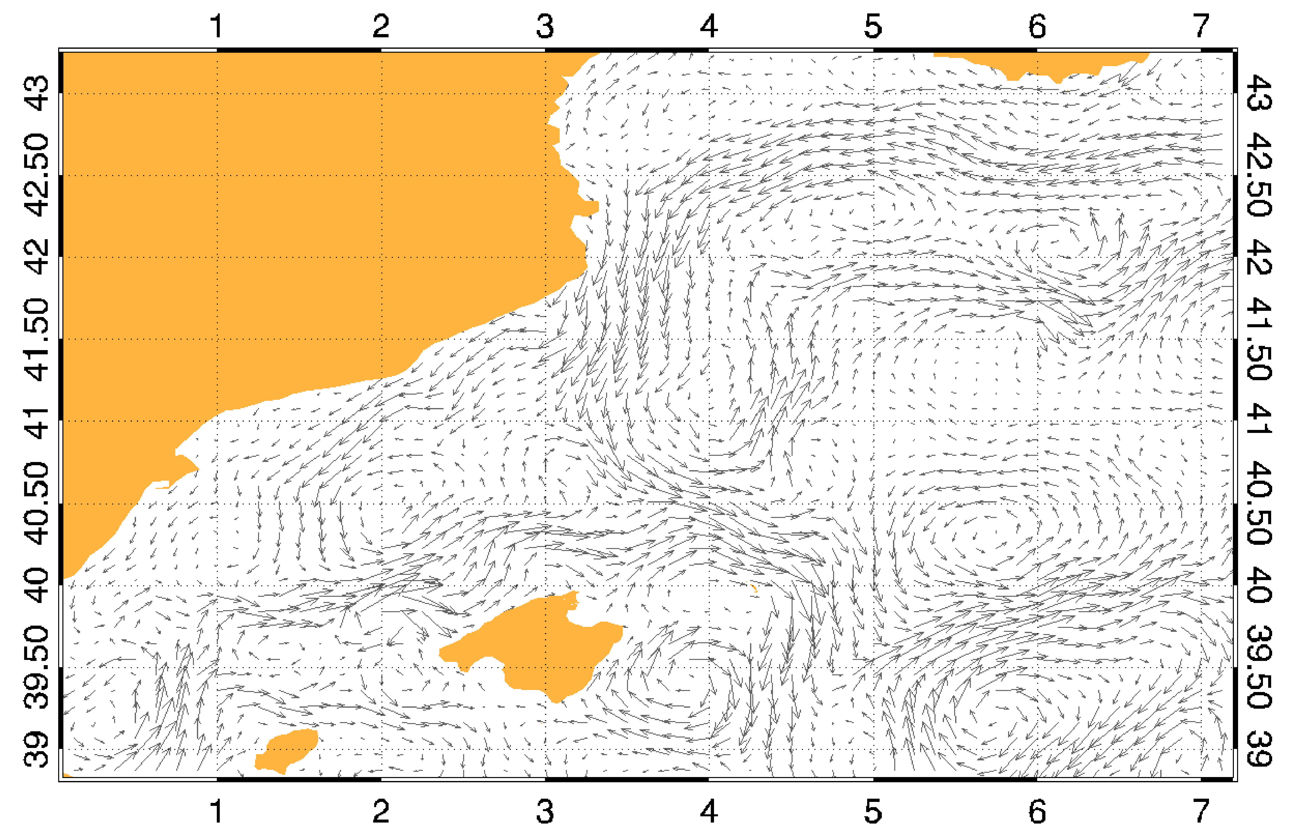
Figure 1: Snapshot of the surface velocity field of the Balearic Sea corresponding to day $640$ in the DieCAST simulation.

II Definition and implementation of FSLEs

FSLEs provide a measure of dispersion as a function of the spatial resolution, serving to isolate the different regimes corresponding to different length scales of oceanic flows, as well as identifying the LCSs present in the data. To calculate the FSLEs we have to know the trajectories of fluid particles, which are computed by integrating the equations of motion for which we need the velocity data $(u,v)$. FSLE are computed from $\tau$, the time required for two particles of fluid (one of them placed at $(x,y)$) to separate from an initial (at time $t$) distance of $\delta_{0}$ to a final distance of $\delta_{f}$ , as:

$$\Lambda(x,y,t,\delta_{0},\delta_{f})\;=\;\frac{1}{\tau}\log\frac{\delta_{f}}{\delta_{0}}.$$ (1)

In principle obtaining $\Lambda(x,y,t,\delta_{0},\delta_{f})$ would imply to consider all the trajectories starting from points at distance $\delta_{0}$ from our basis point; in practice, when confronted with regular, discretized grids, only the four closest neighbors are considered. It is convenient to choose $\delta_{0}$ to be the intergrid spacing among the points on which the FSLEs will be computed, i.e., it is the resolution of the “FSLE grid”. The details of the calculation of the FSLEs are in Appendix A.

III Effect of sampling scale on FSLEs

Notice that we distinguish two types of grids, namely the FSLE grid (in the following “F-grid”) and that where the velocity field is given (called velocity grid or “V-grid”). These two grids need not to coincide. We explore first the effect of changing the resolution of FSLE grid.

In Figure 2 we show an example of the FSLEs derived using four different F-grids with increasing resolutions. Visually, as the resolution of the F-grid is increased the structures already observed in the coarser version are kept, just increasing their detail level. In addition, when resolution is increased, new less active structures are appearing in areas previously regarded as almost inactive. Taking a F-grid finer than the associated V-grid would make no sense if FSLE was an Eulerian measure obtained from single snapshots of the velocity field. But FSLE is a Lagrangian measure, i.e. they are computed using trajectories which integrate information on the history of the velocity field. This allows capturing the effects of the large scales on scales smaller than the V-grid. This does not mean that we reconstruct all the effects taking place at the smaller scales, but only the ones that have been originated by the relatively large velocity features which are resolved on the V-grid.

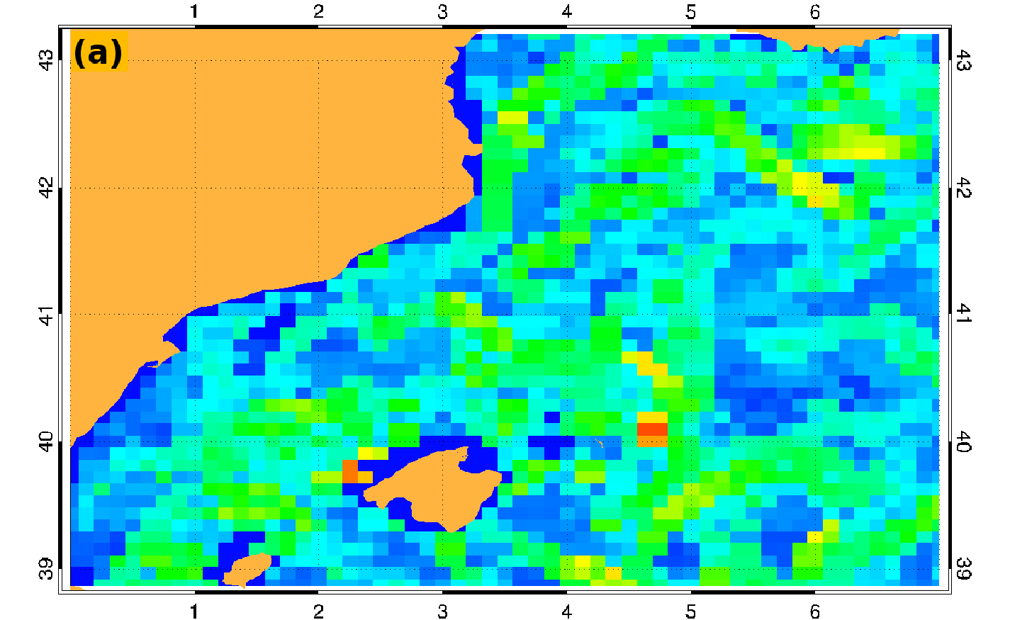
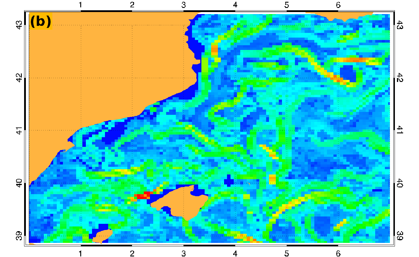
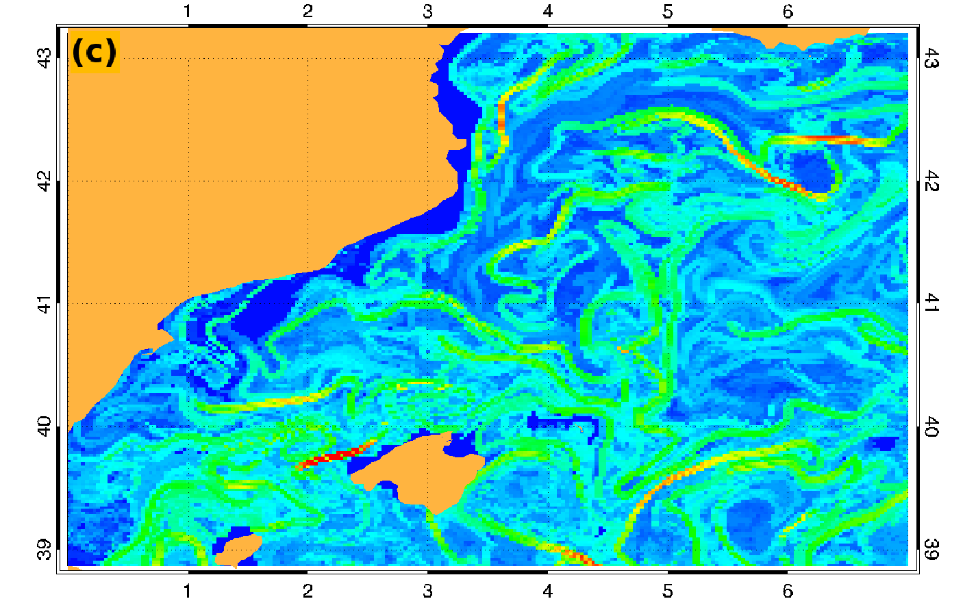
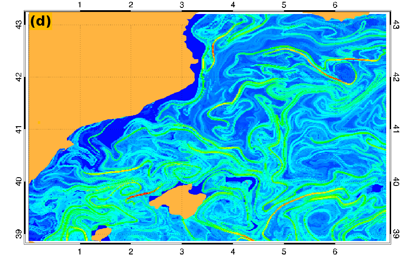
Figure 2: Snapshots of FSLEs backward in time starting from day $640$ at different F-grid resolutions: a) $\delta_{0}=1/8^{\circ}$, b) $\delta_{0}=1/16^{\circ}$, c) $\delta_{0}=1/32^{\circ}$, d) $\delta_{0}=1/64^{\circ}$. In all of them we take $\delta_{f}=1^{\circ}$. The values in the color bar have units of $day^{-1}$.

The main structures of the flow, which are essentially filaments, become finer as resolution is increased, behaving much like the geometrical persistence of a fractal interface Falconer.1990 . The question naturally rises about the possible multifractal character of FSLEs. Multifractality is a property characteristic to turbulent flows, and it is associated to the development of a complex hierarchy accross which energy is transmitted and utterly dissipated Frisch.1995 ; Turiel.2008 . The study of the scaling properties of the distribution of FSLEs at the different resolution scales reveal that they are multifractal (see Appendix B). This implies that changes in scale are accounted for by a well-defined transformation, namely a cascade multiplicative process Frisch.1995 ; Turiel.2008 . It also implies that information is hierarchized Turiel.2002 and so what is obtained first, at the coarsest scales, is the most relevant information. Due to multifractality, small-scale structures, as unveiled by the FSLEs, with typical sizes smaller than that of the velocity resolution, are determined by the larger ones and the multi-scale invariance properties. Thus, no artificiality is induced by this calculation and the robustness of FSLE analysis under changes in scale is confirmed.

A different question concerns the robustness of FSLEs when the V-grid is changed. For instance, when a diagnosis is obtained with a low-resolution velocity field, is this diagnosis compatible with a later improved observation of the velocity? The answer is yes. In Figure 3 we show the FSLEs obtained at a fixed F-grid resolution of $1/8^{\circ}$ for varying velocity resolutions (namely, $1/8^{\circ}$, $1/4^{\circ}$ and $1/2^{\circ}$). The change of resolution of the velocity grid is performed as indicated in Appendix C. We observe that the global features observed with the coarser resolution V-grid are kept when this is refined. Obviously, as the velocity field is described with enhanced resolution new details (with short-range effect on the flow structure and so no contradicting the large-scale picture) become apparent in the FSLEs. However, the effect of refining the V-grid is not only introducing new small-scale structures: there is a consistent increase in the values of the FSLEs as the V-grid is refined. The histograms of the FSLEs, $\Lambda_{f}$, for a given velocity resolution conditioned by the FSLEs, $\Lambda_{c}$, obtained from a coarser velocity field are shown in Figure 4. The modal line (the line of maximum conditioned probability) is close to a straight line. The best linear regression fits are $\Lambda_{1/8^{\circ}}=1.08\Lambda_{1/4^{\circ}}+0.05$ (correlation coefficient, $\rho=0.69$) and $\Lambda_{1/4^{\circ}}=0.99\Lambda_{1/2^{\circ}}+0.04$ ($\rho=0.69$). According to these results, we can approximate the finer FSLEs $\Lambda_{f}$ in terms of the coarser FSLEs $\Lambda_{c}$ as:

$$\Lambda_{f}(\vec{x})\;=\;\Lambda_{c}(\vec{x})\>+\>\Delta\Lambda_{fc},$$ (2)

where the quantity $\Delta\Lambda_{fc}$ determines the contribution to the FSLE by the small-scale variations in velocity not accounted for by the lower resolution version of this field. It is hence independent of $\Lambda_{c}$, so the intercept of the vertical axis with the linear regression equals the mean of this quantity.

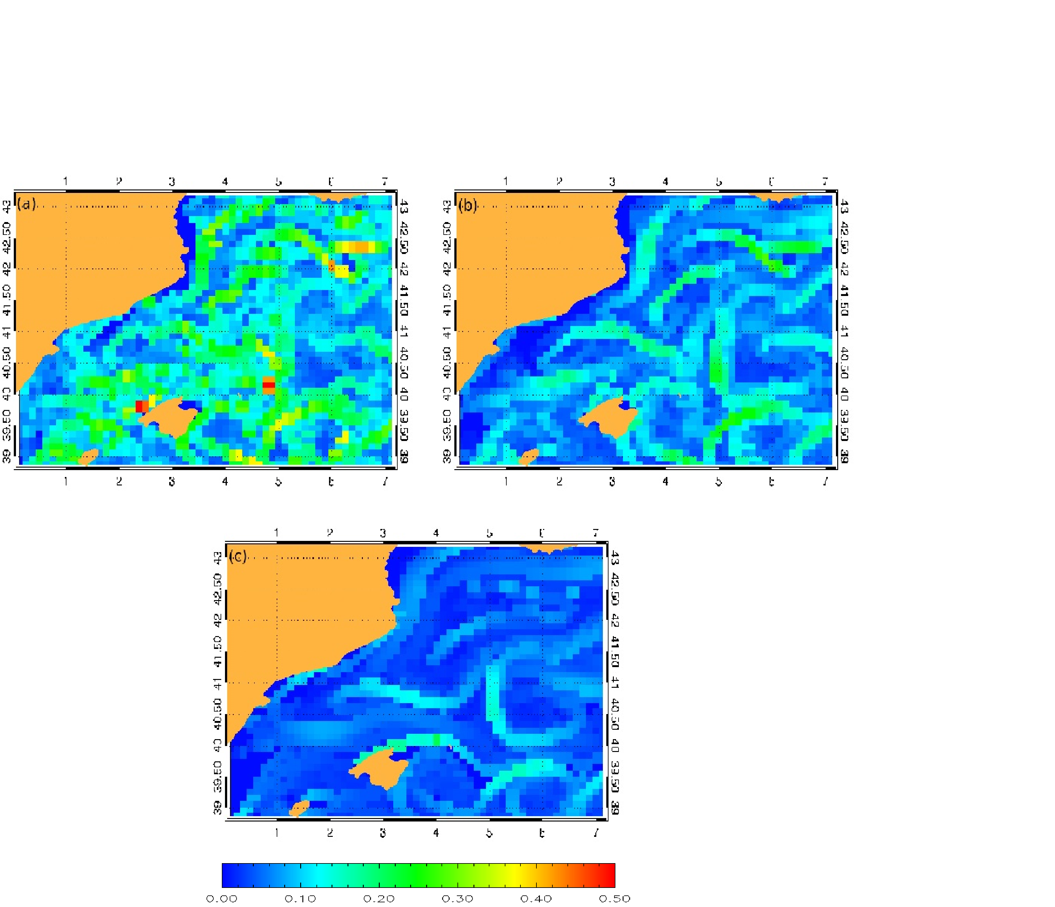
Figure 3: Snapshots of FSLEs backward in time starting from day $640$ at different initial V-grid resolutions: a)$\Delta_{0}=1/8^{\circ}$, b) $\Delta_{0}=1/4^{\circ}$, c) $\Delta_{0}=1/2^{\circ}$. In all of them we take the same F-grid resolution of $\delta_{0}=1/8^{\circ}$, and $\delta_{f}=1^{\circ}$. The color bar has units of day^-1.

A linear dependence of $\Lambda_{f}$ with $\Lambda_{c}$ when scale is changed implies that FSLEs follow a multiplicative cascade Turiel.2006 ; Turiel.2008 , an essential ingredient in multifractal systems which gives further confirmation to our previous results. We have hence shown that a) the dependence of FSLEs on both types of scale parameters reveals a multifractal structure; b) what is diagnosed at the coarser scales is still valid when scale is refined (although as V-grid resolution is increased the reference level of FSLEs is increased by a constant).

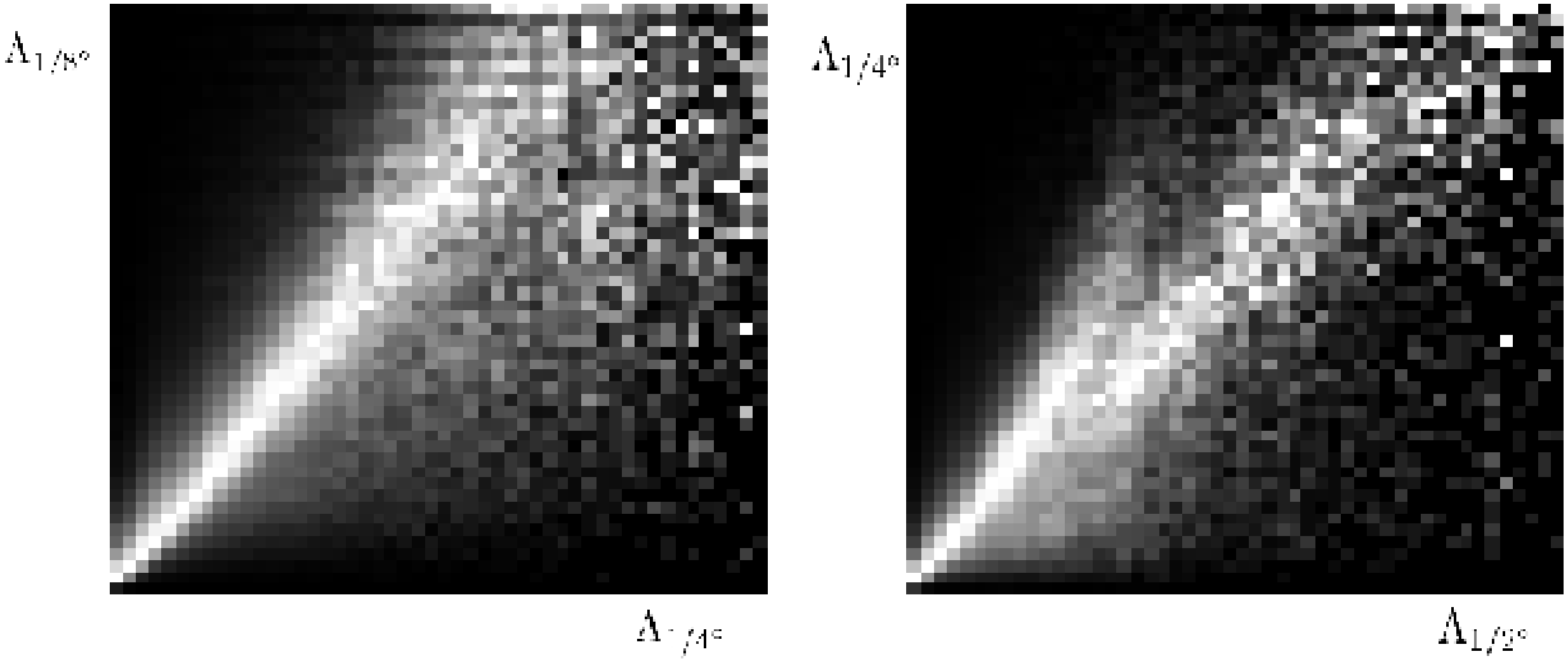
Figure 4: Probability distributions (coded as grey levels) of FSLEs derived at a coarse velocity resolution ($\Lambda_{c}$, vertical axis) conditioned by a finer velocity grid ($\Lambda_{f}$, horizontal axis). The range of values of both axes run linearly from $0$ to $0.5$ day^-1. To obtain a statistics large enough, we have considered $30$ FSLEs snapshots, starting form $t=640$ up to $t=1075$ days, in steps of $15$ days. The brightest color (pure white) corresponds to the maximum probability at each column; the darkest color (pure black) corresponds to zero. Left panel: FLSEs derived from $1/4^{\circ}$ velocities conditioned by FSLEs at original $1/8^{\circ}$ velocities. Right panel: FSLEs from $1/2^{\circ}$ velocities conditioned by FSLEs from $1/4^{\circ}$ velocities.

IV Effect of noise on FSLEs

We compute the FSLEs after applying a random perturbation to all components of the velocity field. The velocity is changed from $(u,v)$ to $(u^{\prime},v^{\prime})$, with $u^{\prime}(x,t)=u(\textbf{x},t)(1+\alpha\eta_{x}(\textbf{x},t))$ and $v^{\prime}(\textbf{x},t)=v(\textbf{x},t)(1+\alpha\eta_{y}(\textbf{x},t))$. $\{\eta_{x}(\textbf{x},t),\eta_{y}(\textbf{x},t)\}$ are sets of Gaussian random numbers of zero mean and unit variance. $\alpha$ measures the relative size of the perturbation (it gives the ratio of the mean amplitude of noise with respect to mean amplitude of the velocity). We introduce three different kinds of error: uncorrelated noise, i.e. different and uncorrelated values of $\{\eta_{x}(\textbf{x},t),\eta_{y}(\textbf{x},t)\}$ for each x and $t$; correlated in time and uncorrelated in space (uncorrelated for different x but the same values at given x for different $t$); and correlated in space and uncorrelated in time (uncorrelated values for different $t$, but the same values for different x at fixed $t$). Note that the perturbation is proportional to the original velocity. Figure 5 shows a snapshot of FSLEs for the velocity field perturbed by uncorrelated noise of a relative size $\alpha=10$, i.e., noise is $10$ times larger than the amplitude of the initial velocity field. The computed Lagrangian structures look rather the same, despite the large size of the perturbation introduced.

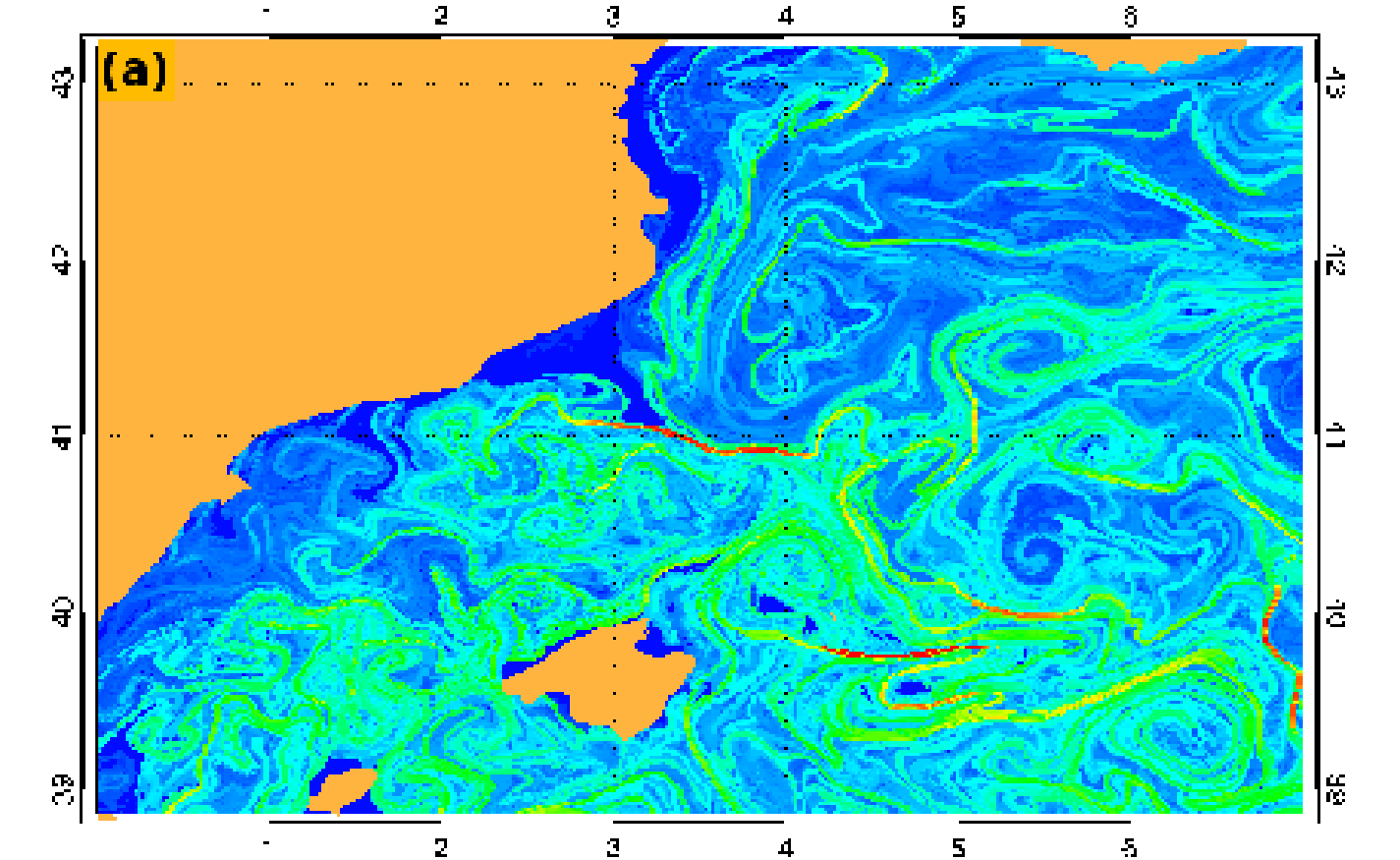
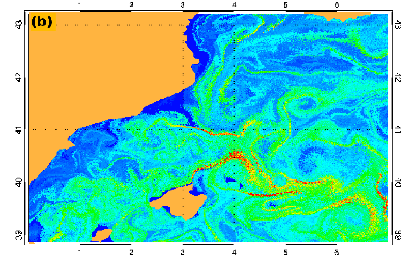
Figure 5: Snapshots of FSLEs calculated backwards in time starting from day $600$ at fixed spatial resolution ($\delta_{0}=1/64^{\circ}$), and at different $\alpha$: a)$\alpha=0$, b) $\alpha=10$. In both of them we take $\delta_{f}=1^{\circ}$. The color bar has units of $day^{-1}$. Initial conditions for which the separation $\delta_{f}$ has not been reached after $600$ days are assigned a value $\Lambda=0$.

In order to quantify the influence of the velocity perturbation in the FSLE calculation we compute the relative error (RE) of perturbed FSLEs with respect to unperturbed FSLEs, $<\epsilon(t)>$, at a given instant of time, and then averaging in time (we have $M=100$ snapshots $:t=t_{1},...,t_{M}$) as:

$$\epsilon(t_{i})=\sqrt{\frac{1}{N}\sum_{\textbf{x}}\dfrac{|\Lambda^{\alpha}(\textbf{x},t_{i})-\Lambda(\textbf{x},t_{i})|^{2}}{|\Lambda(\textbf{x},t_{i})|^{2}}},\ \ \ \hfill<\epsilon(t)>\equiv\frac{1}{M}\sum_{i=1}^{M}\epsilon(t_{i})\ .$$ (3)

$\Lambda(\textbf{x},t_{i})$ and $\Lambda^{\alpha}(\textbf{x},t_{i})$ are the FSLEs fields without and with inclusion of the perturbation in the velocity data, respectively. The sum over x runs over the $N=2679$ spatial points. Figure 6 shows the average RE as a function of $\alpha$. It must be remarked that the RE has always small values: even for $\alpha=10$ the RE remains smaller than $0.23$ for the three kinds of noise. To get an idea of how relevant these quantities are, we have computed the RE of shuffled FSLEs (permuting locations at random) with respect to the original ones, and obtained a value of $1.143$. FSLEs are thus robust against uncorrelated noise; the reason is the averaging effect produced when computing them by integrating over trajectories which extend in time and space, that tends to cancellate random, uncorrelated errors.

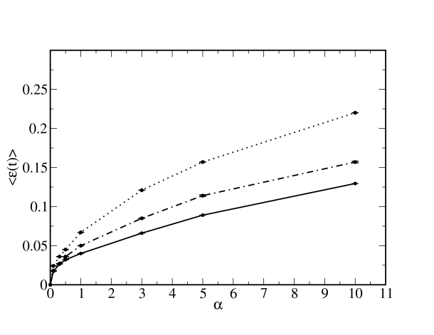
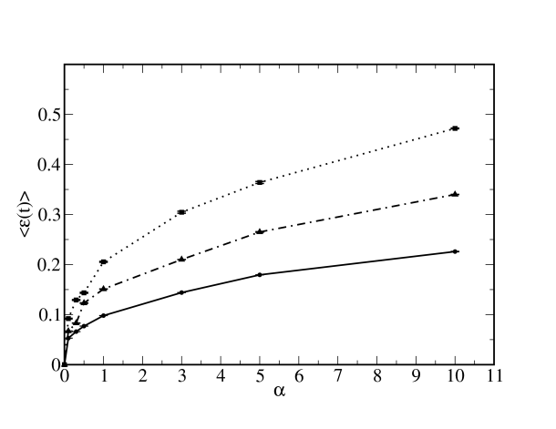
Figure 6: Relative error $<\epsilon(t)>$ of the FSLE fields for different perturbation intensity $\alpha$ in the velocity data. Solid line is for uncorrelated noise in space and time, dashed-dotted line is for uncorrelated noise in time and correlated in space, and dotted line is for uncorrelated noise in space and correlated in time. $<\epsilon(t)>$ is obtained by averaging the RE in $100$ snapshots (see Eq. (3)). The error bar is the statistical error of the temporal average $<\epsilon(t)>$. Left: spatial resolution $\delta_{0}=1/8^{\circ}$. Right: spatial resolution $\delta_{0}=1/64^{\circ}$. In all calculations we take $\delta_{f}=1^{\circ}$

Now we proceed by adding noise to the particle trajectories. This is a simplified way of including unresolved small scales in the Lagrangian computations Griffa.1996 . To be precise we solve numerically the system of Equations (13) and (14) (see Appendix D), where a stochastic term with a Gaussian random number and an effective eddy-diffusion, $D$, has been added. For the diffusivity we use Okubo’s empirical formula Okubo.1971 , which relates the effective eddy-diffusion, $D$ in $m^{2}/s$, with the spatial scale, $l$ in meters: $D(l)=2.055\ 10^{-4}\ l^{1.15}$. If we take $l=12\ km$, which is the approximate length corresponding to the $1/8^{\circ}$ DieCAST resolution at Mediterranean latitudes, we obtain $D\sim 10\ m^{2}s^{-1}\equiv D_{0}$.

In Figure 7 we show particle trajectories without (top panel) and with (bottom panel) eddy diffusion. As expected diffusion introduces small scale irregularities on the trajectories, and also substantial dispersion at large scales. In Figure 8, FSLEs with $\delta_{0}=1/64^{\circ}$ $D=0~{}m^{2}s^{-1}$ and $D=0.9~{}m^{2}s^{-1}$ (obtained for this scale by Okubo’s formula for spatial resolution) are shown. We can see that the main mesoscale structures are maintained, but small-scale filamental structures are lost since filaments become blurred. This is somehow expected a priory because diffusion introduces a new length scale $l_{D}$ proportional to $\sqrt{D}$. A pointwise comparison of noiseless and noise-affected FSLEs makes no sense, since the noise-induced blurring disperses FSLEs values specially at places with low values, see Figure 8. But for Lagrangian diagnostics high FSLE values are much more relevant, so we compute the error restricted to the places where $\Lambda>0.2$ for $D=0$. Left panel of Figure 9 shows the RE respect to the $D=0$ case (applying Equation (3)) for different values of $D$. The RE monotonously increases with $D$, but remains smaller than $0.6$ for the largest value of $D$ considered. Again, to get an idea of how relevant these relative errors are, we have to compare them with the RE of shuffled FSLEs, of value $1.143$.

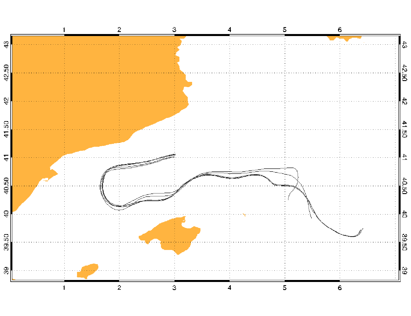
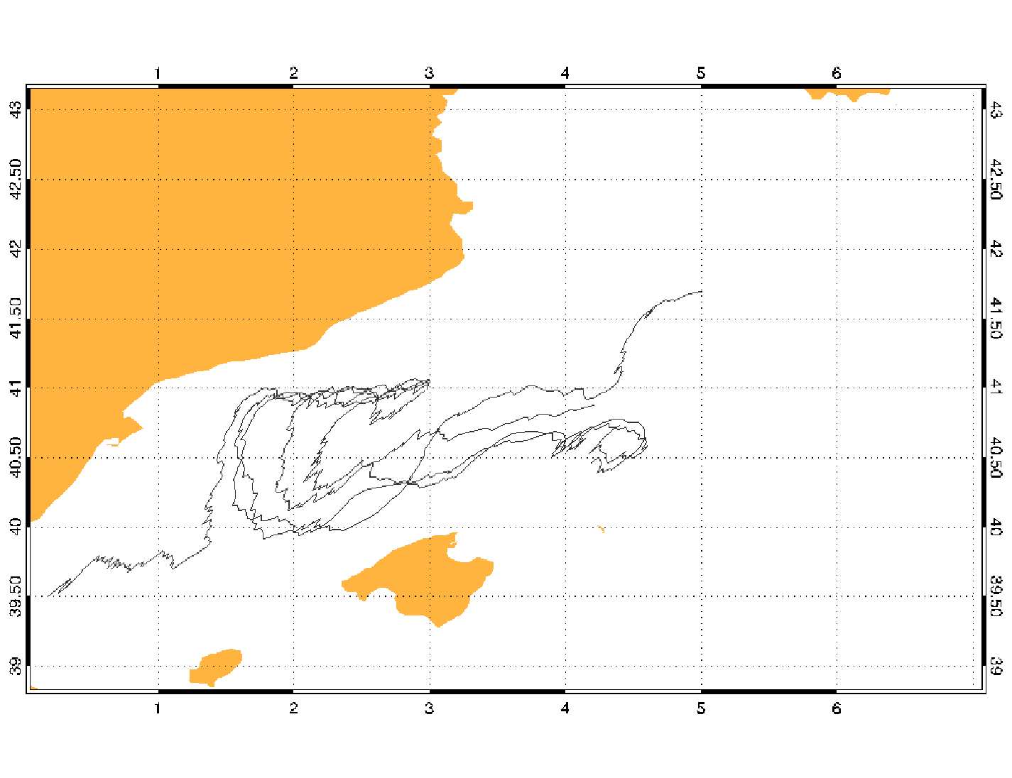
Figure 7: Trajectories of five particles without diffusion (top) and with diffusion (bottom). The difference in the initial positions of all five particles is about $0.06^{\circ}$, and we use these initial conditions in both computations. The trajectories were computed for $50$ days of integration. We used the eddy-diffusion $D_{0}\sim 10m^{2}s^{-1}$ assigned by the Okubo formula to the resolution of the DieCAST model at Mediterranean latitudes.

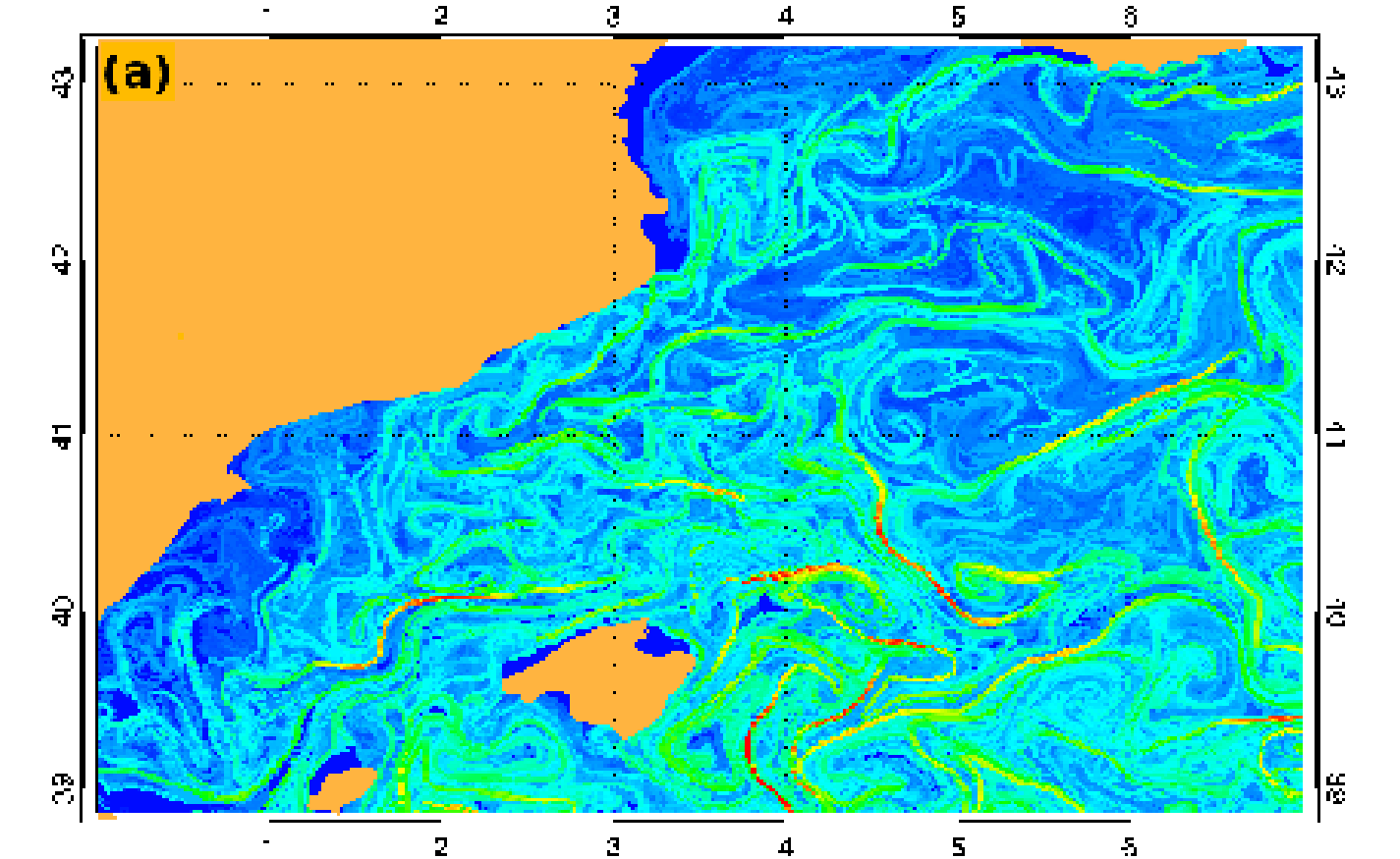
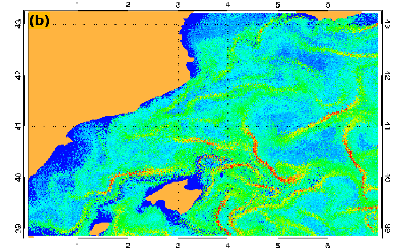
Figure 8: FSLEs computed backwards from day $500$ at the same spatial resolution ($\delta_{0}=1/64^{\circ}$), and for different eddy-diffusion values: a)$D=0~{}m^{2}s^{-1}$ b) $D=0.9~{}m^{2}s^{-1}$. We take $\delta_{f}=1^{\circ}$. The color bar has units of $day^{-1}$. Initial conditions for which the separation $\delta_{f}$ has not been reached after $500$ days are assigned a value $\Lambda=0$.

As a matter of fact, diffusion introduces an effective observation scale, and one should not go beyond that limit to obtain senseful results; this is illustrated in the right panel of Figure 9. As shown in the figure, for fixed eddy diffusivity (in the case of the figure, $D_{0}=10m^{2}s^{-1}$), when $\delta_{0}$ becomes greater the error diminishes. Hence, a fixed diffusion will eventually be negligible at a scale large enough, in this way determining an observation scale. A completely different situation is given when the eddy-diffusion depends on the scale according to Okubo’s formula (in our case, at $\delta_{0}=1/16^{\circ}$ $D=4,5m^{2}s^{-1}$; at $\delta_{0}=1/32^{\circ}$ $D=2m^{2}s^{-1}$; and at $\delta_{0}=1/64^{\circ}$, $D=0.9m^{2}s^{-1}$). Now $<\epsilon(t)>$ takes a constant value close to $0.45$, meaning that Okubo’s diffusion behaves the same at all scales. This is expected since Okubo’s law is based on the hypothesis that unsolved scales act as diffusers, like in turbulence Frisch.1995 . Our result is consistent with the ideas behind Okubo’s hypothesis.

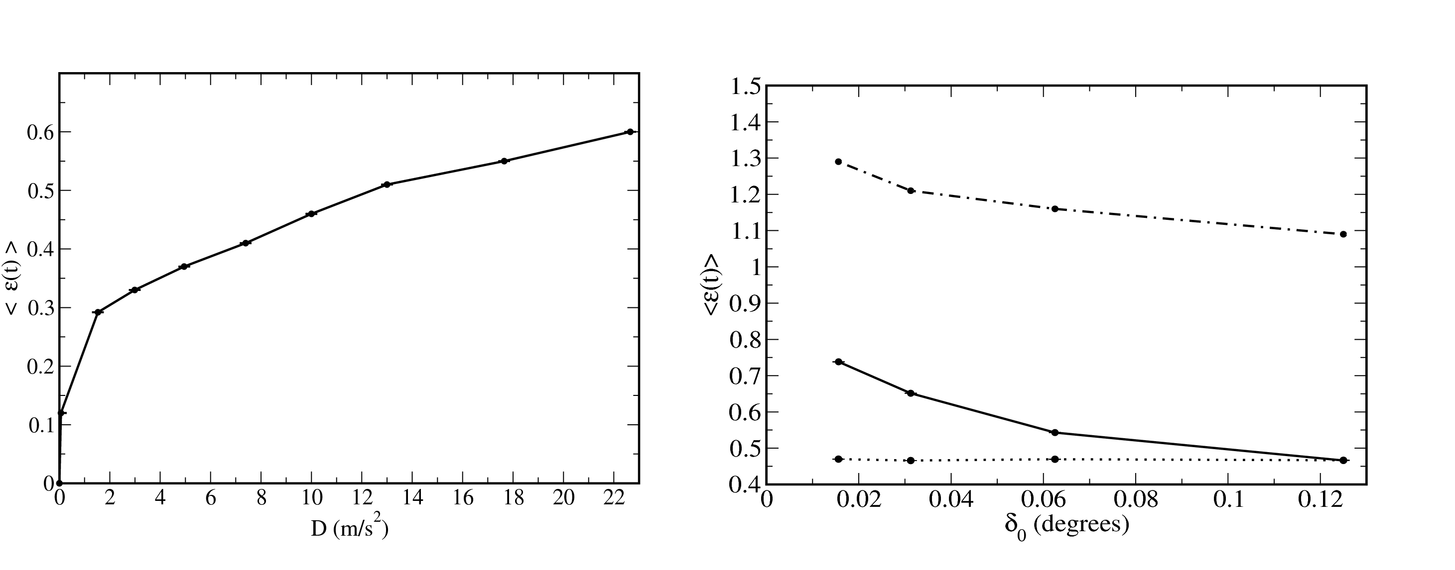
Figure 9: Left: Relative error $<\epsilon(t)>$ of the FSLE at the different values of $D$ in the particle trajectories, with respect to the $D=0$ case. Spatial resolution is $\delta_{0}=1/8^{\circ}$, and $\delta_{f}=1^{\circ}$. $<\epsilon(t)>$ is obtained by temporally averaging the relative errors in $100$ snapshots. The (small) error bars indicate the statistical error in the $<\epsilon(t)>$ average. Right: Dotted line is the RE $<\epsilon(t)>$ of the FSLE at different spatial resolution $\delta_{0}$ and at one assigned eddy-diffusion $D$ for every spatial resolution in the particle trajectories with respect to the $D=0$ case. Solid line is the RE $<\epsilon(t)>$ of the FSLE at different spatial resolution $\delta_{0}$, and at the same eddy-diffusion $D_{0}=10m^{2}s^{-1}$ in the particle trajectories with respect to the $D=0$ case. Dashed-dotted line is the RE of shuffled FSLE with respect to the original case ($D=0$) at different spatial resolution. $<\epsilon(t)>$ by temporally averaging the RE in $100$ snapshots. The (small) error bar indicates the statistical error in the $<\epsilon(t)>$ average. In all of them we take $\delta_{f}=1^{\circ}$.

We can characterize the effective diffusion scale from the properties of the histograms. In Figure 10 we present the histograms of FSLEs at different F-grid resolutions, and including or not eddy diffusion which takes always the same value $D_{0}=10m^{2}s^{-1}$. For $\delta_{0}=1/8^{\circ}$ the histograms with and without diffusion are almost coincident. This is due to the fact that the value of diffusion we are using is the one corresponding, by the Okubo’s formula, to $1/8^{\circ}$. i.e., we are parameterizing turbulence below $1/8^{\circ}$, and this has no effects on the FSLE computations if the minimum scale considered is also $1/8$. However, this behavior is different for smaller $\delta_{0}$ (always keeping $D_{0}=10m^{2}s^{-1}$). The histograms for $\delta_{0}=1/16,1/64^{\circ}$, with and without diffusion, are clearly different, those including diffusion becoming closer to the histogram for $\delta_{0}=1/8^{\circ}$.

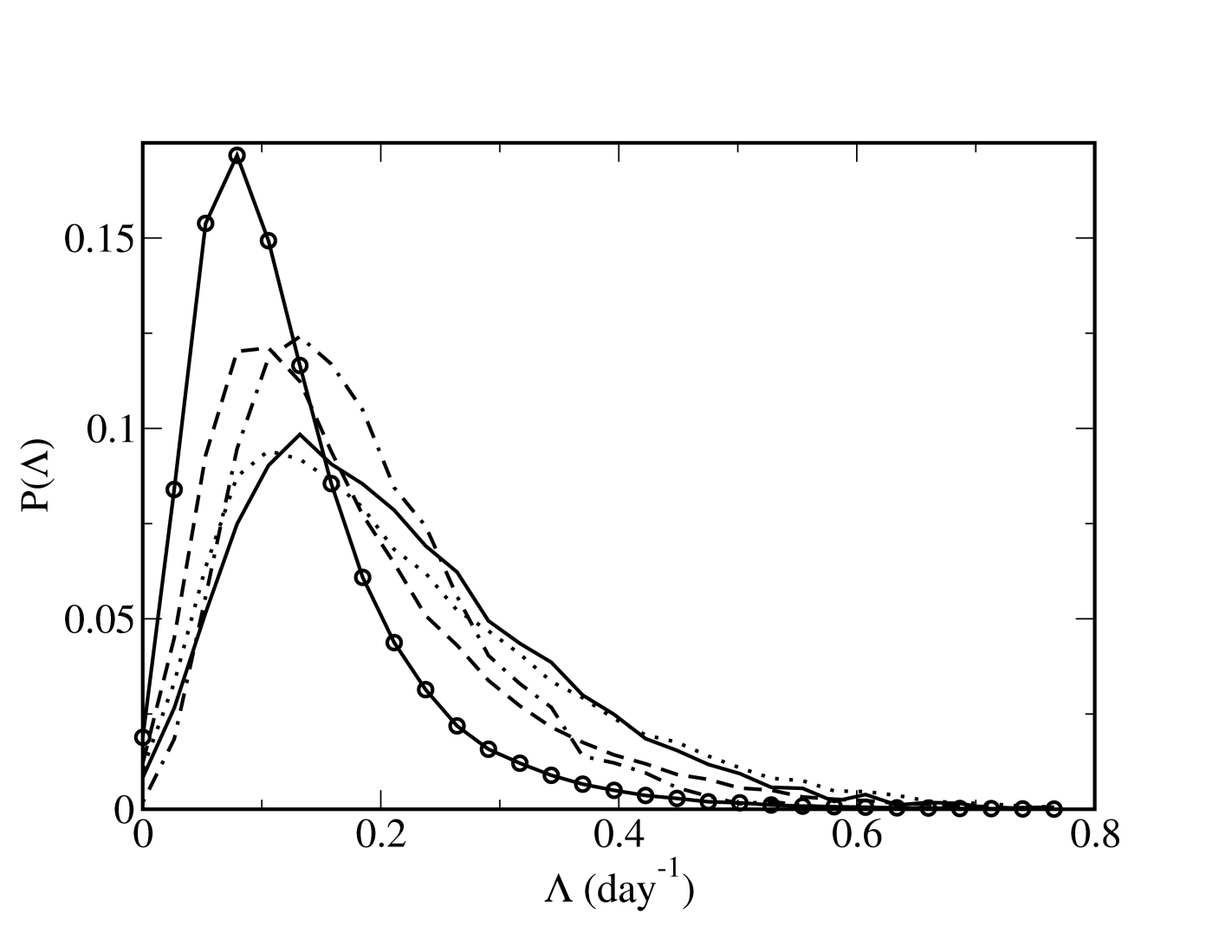
Figure 10: Comparison between probability density function for the FSLEs at different resolutions with different values of eddy-diffusion, and without diffusion. It is obtained from the temporal average ($30$ snapshots) of histograms. Solid line for $\delta_{0}=1/8^{\circ}$ with diffusion, dotted $\delta_{0}=1/8^{\circ}$ without diffusion, dashed $\delta_{0}=1/16^{\circ}$ without diffusion, dashed-dotted line for $\delta_{0}=1/64^{\circ}$ with diffusion, and circle-line for $\delta_{0}=1/64^{\circ}$ without diffusion.

V Conclusions

In this paper, we have analyzed the sensibility of FSLE-based analyses for the diagnostic of Lagrangian properties of the ocean (most notably, horizontal mixing and dispersion). Our sensibility tests include the two most important effects when facing real data, namely dynamics of unsolved scales and of noise. Our results show that even if some dynamics are missed (because of lack of sampling or inaccuracy of any kind in the measurements) FLSEs results would still give an accurate picture of Lagrangian properties, valid for the solved scales. This does not mean that scale and/or noise leave FSLEs unaffected, but the way in which they modify this Lagrangian diagnostics can be properly accounted.

Lagrangian methods provide answers to problems which have a deep impact on risk management (e.g. control of pollutant dispersion) as well as on ecosystem analysis (e.g. tracking nutrient mixing and transport, identifying the role of horizontal mixing in primary productivity). They utterly will give hints about energy exchanges in the upper ocean and will help in understanding processes driving global change in the oceans. The use of Lagrangian techniques for the assessment of the transport and mixing properties of the ocean has grown in importance in the latest years, with increasing efforts devoted to the implementation of appropriate techniques but few studies on the validity of the results when real data, affected by realistic constraints, are used. Our work will serve to unify and interpret the analyses provided by Lagrangian methods when real data are processed.

Appendix A Calculation of FSLE.

It is natural to choose the initial points $(x,y)$ on the nodes of a grid with lattice spacing coincident with the initial separation of fluid particles $\delta_{0}$. In this way one obtains maps of values of $\Lambda$ at a spatial resolution that will coincide with $\delta_{0}$. To compute $\Lambda$ we need to know the trajectories of the particles. The equations of motion that describe the horizontal evolution of particle trajectories in the velocity field are:

$$\frac{d\phi}{dt} = \frac{u(\phi,\lambda,t)}{R\cos{\lambda}},$$ (4)

$$\frac{d\lambda}{dt} = \frac{v(\phi,\lambda,t)}{R},$$ (5)

where $u$ and $v$ represent the zonal and meridional components of the surface velocity field coming from the simulations described above, $R$ is the radius of the Earth (6400 km in our computations). Numerically we proceed integrating Eqs. (4) and (5) using a standard fourth-order Runge-Kutta scheme with an integration time step $dt$ = 6 hours. Spatiotemporal interpolation of the velocity data is achieved by bilinear interpolation. Since this technique requires an equally spaced grid and this is not the case for the spherical coordinates $(\phi,\lambda)$, for which the grid is not uniformly spaced in the latitude coordinate, we first transform it to a new system $(\phi,\mu)$ where the grid turns out to be uniformly sampled Mancho.2008 . The latitude $\lambda$ is related to the new coordinate $\mu$ according to:

$$\mu\;=\;\log|\sec\lambda\>+\>\tan\lambda|$$ (6)

Using the new coordinate variables the equations of motion become:

$$\frac{d\phi}{dt} = \frac{u(\phi,\mu,t)}{R\cos{\lambda(\mu)}}$$ (7)

$$\frac{d\mu}{dt} = \frac{v(\phi,\mu,t)}{R\cos{\lambda(\mu)}},$$ (8)

and one can convert the $\mu$ values back to latitude $\lambda$ by inverting Eq. (6): $\lambda=\pi/2-2\arctan e^{-\mu}$. Once we integrate the equations of motion, Eqs. (7) and (8), we compute the FSLEs applying Eq. (1) for the points of a lattice with spacing $\delta_{0}$. We will only compute FSLEs integrating backwards-in-time the particle trajectories, since LCSs associated to this has a direct physical interpretation, but all our results are similar for forward-in-time dynamics.

Appendix B Multifractal character of FSLE.

To study if FSLEs behave like multifractal systems we have computed their probability density distribution, $P(\delta_{0},\Lambda)$, for different resolutions $\delta_{0}$. It must follow that for any resolution scale $\delta_{0}$ of FSLE grid we should observe:

$$P(\delta_{0},\Lambda)\propto\delta_{0}^{d-D(\Lambda)},$$ (9)

Notice that as $d-D(\Lambda)$ is a positive quantity, $P(\delta_{0},\Lambda)$ becomes smaller as $\delta_{0}$ is reduced. In fact, a characteristic signature of multifractal scaling is having a scale-dependent histogram which becomes more strongly peaked as the resolution scale becomes smaller. We know that there is a FSLE for each domain point, so we can normalize the FSLE distribution by its maximum (that will be attained for a value $\Lambda_{c}$) and then retrieve the associated singularity spectrum according to the following expression:

$$D(\Lambda)\;=\;d-\frac{\log{\frac{P(\delta_{0},\Lambda)}{P(\delta_{0},\Lambda_{c})}}}{\log{\delta_{0}}}.$$ (10)

In Figure 11, top, we show the histograms (averaged over $30$ snapshots distributed among $15$ months) normalized to have the same unitary are. One can see that when the resolution gets finer the $P(\delta_{0},\Lambda)$ narrows, and the peak height increases, in agreement with Equation (9). According to the definition of Microcanonical Multifractals Isern.2007 ; Turiel.2008 , the system will be multifractal if the curves $D(\Lambda)$ estimated at different resolutions $\delta_{0}$ using Equation (10) are all equal. This can be observed in Figure 11, bottom. The collapse of the four curves is not perfect due to the lost of translational invariance produced by the small size of the domain -the Balearic basin- that we analyze. Thus, the interfaces of constant $\Lambda$ values build an approximate multifractal hierarchy and generalized scale invariance is present in the FSLE field.

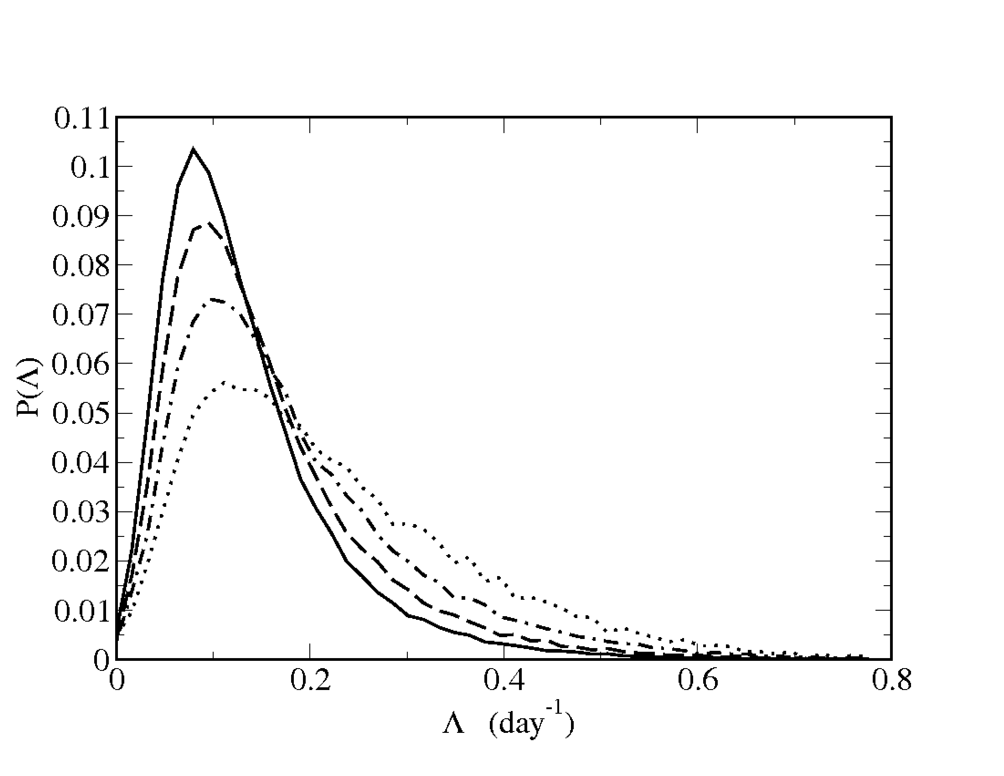
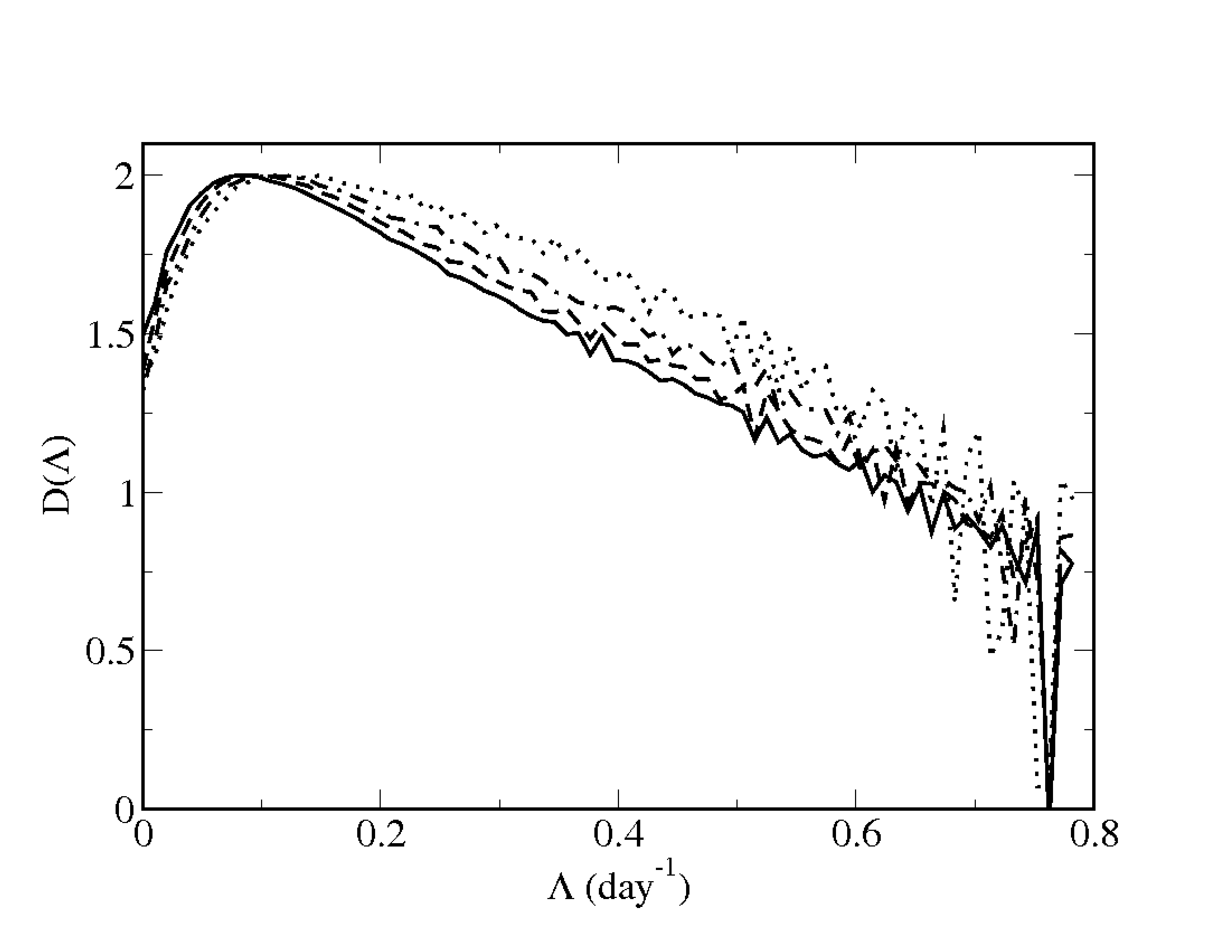
Figure 11: Top: Comparison of the probability density functions $P(\delta_{0},\Lambda)$ for the FSLEs at different resolutions. It is obtained from the temporal average ($30$ snapshots) of histograms. Dotted line is for $\delta_{0}=1/8^{\circ}$, dashed-dotted line $\delta_{0}=1/16^{\circ}$, dashed $\delta_{0}=1/32^{\circ}$, and solid line for $\delta_{0}=1/64^{\circ}$. Bottom: $D(\Lambda)$ for different values of $\delta_{0}$. Dotted for $\delta_{0}=1/8^{\circ}$, dashed-dotted line $\delta_{0}=1/16^{\circ}$, dashed $\delta_{0}=1/32^{\circ}$, and solid line line for $\delta_{0}=1/64^{\circ}$.

Appendix C Change of resolution of the velocity grid.

In order to reduce the resolution of a given velocity grid, the easiest way would be by subsampling the existing grid points or by block-averaging the values of the velocity and assign the result to the central grid point. However, in the case of a complex boundary such as the Mediterranean coast such a strategy is strongly inconvenient, as the coarsening of the grid would imply to change land circulation barriers (islands, straits). The disappearance of a land barrier or the creation of a new one as a consequence of the coarsening would imply a dramatic change in the value of FSLEs at all points affected by the modified circulation; if the circulation patterns are rather complex almost every point could be affected. We have thus preferred to smooth the velocity with a convolution kernel weighted with a local normalization factor, and keeping the original resolution for the data so land barriers are equally well described than in the original data.

We define the coarsening kernel of scale factor $s$, $\kappa_{s}$, as:

$$\kappa_{s}(x,y)\;=\;e^{-\frac{x^{2}+y^{2}}{2s^{2}}}$$ (11)

We disregard the introduction of a normalization factor at this point since we will need to normalize locally later. The coarsened version of the velocity vector would hence be given by the convolution of this kernel with the velocity, denoted by $\kappa_{s}\star\vec{v}$. A coarsening convolution kernel turns out to be convenient with almost horizontal fields, as the derivatives commute with the convolution operator so if $\nabla\vec{v}\approx 0$ hence $\kappa_{s}\star\nabla\vec{v}\approx 0$. However, this coarsening scheme needs to be improved. By convention, we take the velocity $\vec{v}$ as zero over land points. For that reason, a simple convolution does not produce a correct coarsened version of the velocity because points close to land would experience a loss of energy. The easiest way to correct this is to normalize by the weight of the sea points. Let us first define the sea mask $M(x,y)$ as $1$ over the sea and $0$ over the land. The normalization weight is given by $\kappa_{s}\star M$. For points very far from the land, this weight is just the normalization of $\kappa_{s}$. For points surrounded by land points the weight takes the contributions from sea points only. We thus define the coarsened version by a scale factor $s$ of the velocity, $\vec{v}_{s}$, as:

$$\vec{v}_{s}\;=\;\frac{\kappa_{s}\star\vec{v}}{\kappa_{s}\star M}$$ (12)

In Figure 12 we show two examples of coarsened velocities. We can see that typical circulation patterns are coarsened as $s$ increases, while land obstacles are preserved. In fact, if $\Delta_{0}$ is the velocity resolution scale, the effective resolution scale of $\vec{v}_{s}$ is $s\Delta_{0}$ (the nominal resolution, on the contrary, is the original one, $\Delta_{0}$).

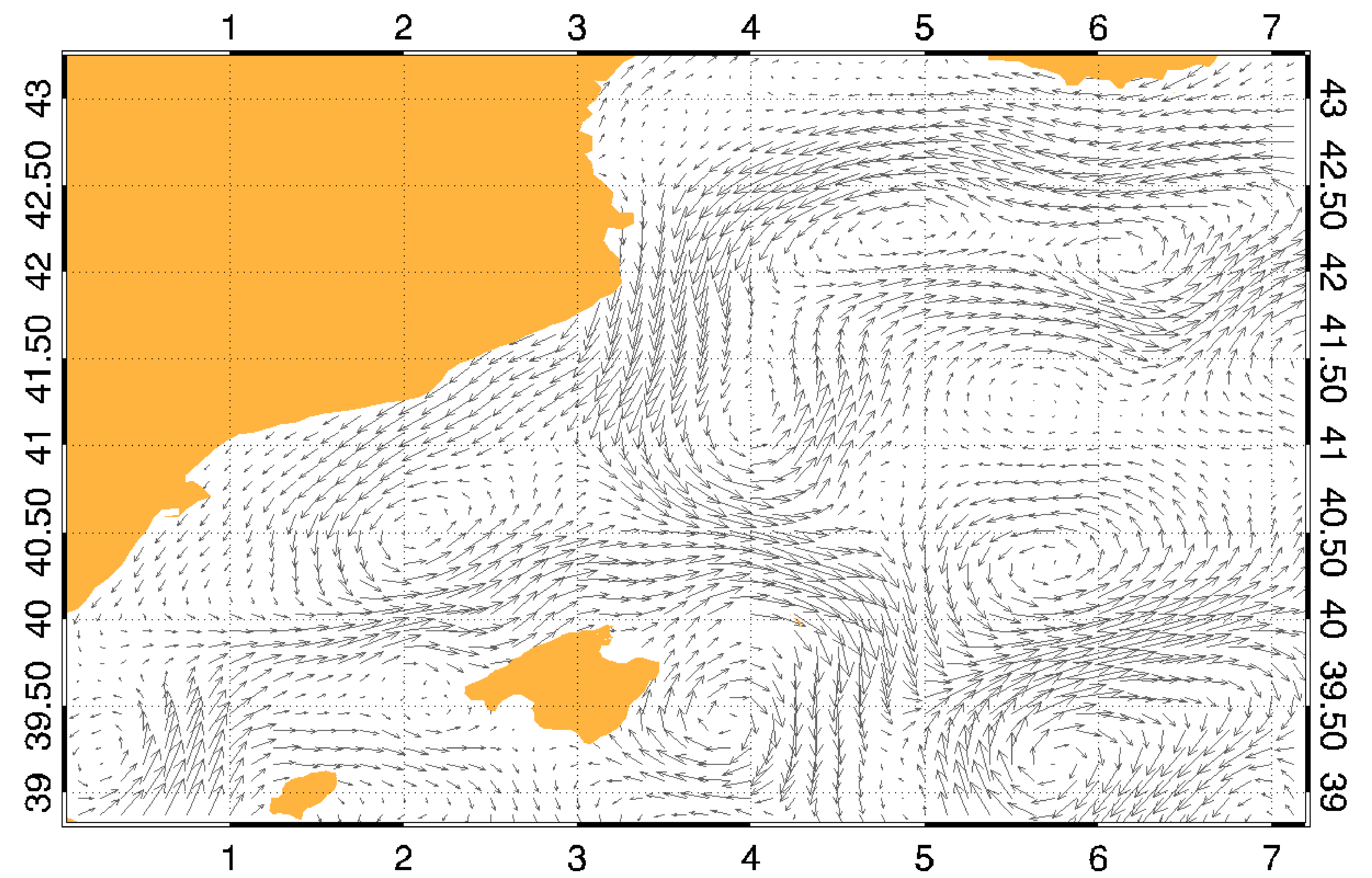
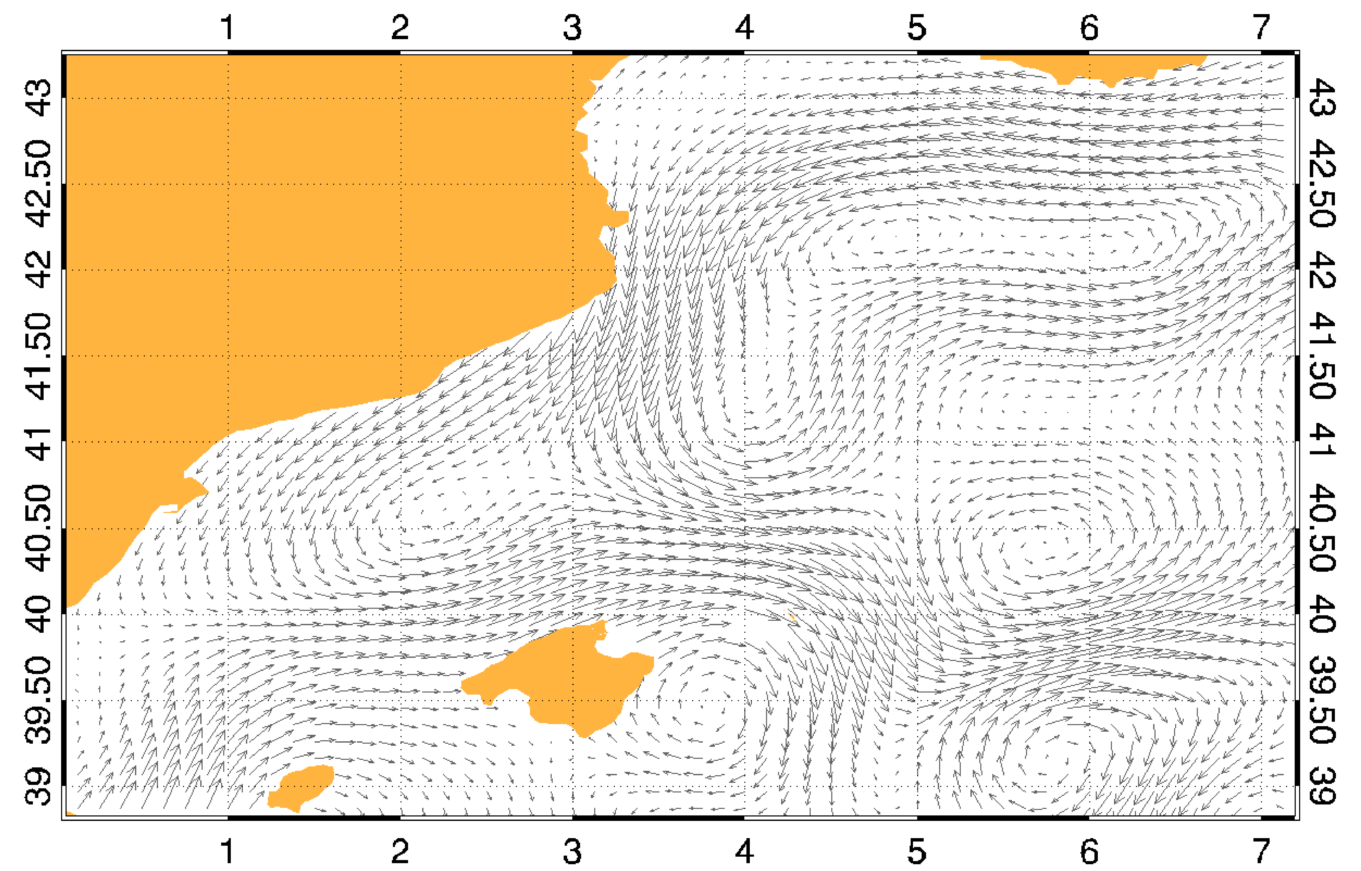
Figure 12: Top: Velocity field coarsened by a scale factor $s=2$, for a equivalent resolution $\delta_{0}=1/4^{\circ}$. Bottom: Velocity field coarsened by a scale factor $s=4$, for a equivalent resolution $\delta_{0}=1/2^{\circ}$.

Appendix D Introducing noise in the particle’s trajectories.

In order to introduce noise in the particle’s trajectories we resolve the following system of stochastic equations:

$$\frac{d\phi}{dt}=\frac{u(\phi,\lambda,t)}{R\cos(\lambda)}+\frac{\sqrt{2D}}{R\cos(\lambda)}\xi_{1}(t),$$ (13)

$$\frac{d\lambda}{dt}=\frac{v(\phi,\lambda,t)}{R}+\frac{\sqrt{2D}\xi_{2}(t)}{R}.$$ (14)

$\xi_{i}(t)\ \ i=1,2$ are the components of a two-dimensional Gaussian white noise with zero mean and correlations $<\xi_{i}(t)\xi_{j}(t^{\prime})>=\delta_{ij}\delta(t-t^{\prime})$.Eqs. (13 and 14) use a simple white noise added to the trajectories. A more realistic representation of small-scale Lagrangian dispersion in turbulent fields requires using other kinds of correlated noises Griffa.1996 but, as we are interested in examining influences of the missing scales, it is convenient to use white noise, since this would represent the extreme case of very irregular trajectories which gives an upper bound to the effects of more realistic smoother small scales. Thus the tests presented here are similar to the ones considered before (perturbation of the velocity) when adding uncorrelated perturbations to the velocity, but here the perturbation acts at arbitrarily small scales, as appropriate for a turbulent field, instead of being smooth below a cutoff scale, as appropriate for modelling observational errors.

References

- (1) V. Artale, G. Boffetta, A. Celani, M. Cencini, and A. Vulpiani. Dispersion of passive tracers in closed basins: Beyond the diffusion coefficient. Physics of Fluids, 9:3162–3171, 1997.
- (2) E. Aurell, G. Boffetta, A. Crisanti, G. Palading, and A. Vulpiani. Predictability in the large: an extension of the concept of Lyapunov exponent. Journal of Physics A, 30:1–26, 1997.
- (3) F.J. Beron-Vera, M.J. Olascoaga, and G.J. Goni. Oceanic mesoscale eddies as revealed by Lagrangian coherent structures. Geophysical Research Letters, 35:L12603, 2008.
- (4) G. Boffetta, G. Lacorata., G. Redaelli, and A. Vulpiani. Detecting barriers to transport: a review of different techniques. Physica D, 159:58–70, 2001.
- (5) G. Buffoni, P. Falco, A. Griffa, and E. Zambianchi. Dispersion processes and residence times in a semi-enclosed basin with recirculating gyres: An application to the Tyrrhenian sea. Journal of Geophysical Research - Oceans, 102:18699–18713, 1997.
- (6) F. d’Ovidio, V. Fernández, E. Hernández-García, and C. López. Mixing structures in the mediterranean sea from finite-size lyapunov exponents. Geophysical Research Letters, 31:L17203, 2004.
- (7) F. d’Ovidio, J. Isern-Fontanet, C. López, E. Hernández-García, and E. García-Ladona. Comparison between Eulerian diagnostics and Finite-Size Lyapunov Exponents computed from altimetry in the Algerian basin. Deep-Sea Research I, 56:15–31, 2009.
- (8) K. Falconer. Fractal Geometry: Mathematical Foundations and Applications. John Wiley and sons, Chichester, 1990.
- (9) V. Fernández, D.E. Dietrich, R.L. Haney, and J. Tintoré. Mesoscale, seasonal and interannual variability in the Mediterranean sea using a numerical ocean model. Progress in Oceanography, 66:321–340, 2005.
- (10) U. Frisch. Turbulence: The legacy of A.N. Kolmogorov. Cambridge Univ. Press, Cambridge MA, 1995.
- (11) A. Garcia-Olivares, J. Isern-Fontanet, and E. Garcia-Ladona. Dispersion of passive tracers and finite-scale Lyapunov exponents in the Western Mediterranean Sea. Deep Sea Research I, 54:253–268, 2007.
- (12) A. Griffa. Applications of stochastic particle models to oceanographic problems. In R. Adler, P. Muller, and B. Rozovskii, editors, Stochastic modelling in physical oceanography. Birkhauser, 1996.
- (13) G. Haller. Finding finite-time invariant manifolds in two-dimensional velocity fields. Chaos, 10(1):99–108, 2000.
- (14) G. Haller and A. Poje. Finite time transport in aperiodic flows. Physica D, 119:352–380, 1998.
- (15) G. Haller and G. Yuan. Lagrangian coherent structures and mixing in two-dimensional turbulence. Physica D, 147:352–370, 2000.
- (16) A. C. Haza, A. C. Poje, T. M. Özgökmena, and P. Martin. Relative dispersion from a high-resolution coastal model of the Adriatic Sea. Ocean Modelling, 22:48–65, 2008.
- (17) J. Isern-Fontanet, A. Turiel, E. Garcia-Ladona, and J. Font. Microcanonical multifractal formalism: application to the estimation of ocean surface velocities. Journal of Geophysical Research, 112:C05024, 2007.
- (18) D. Iudicone, G. Lacorata, V. Rupolo, R. Santoleri, and A. Vulpiani Sensitivity of numerical tracer trajectories to uncertainties in OGCM velocity fields. Ocean Modelling, 4:313-325, 2002.
- (19) B. Joseph and B. Legras. Relation between kinematic boundaries, stirring, and barriers for the antartic polar vortex. Journal of Atmospheric Sciences, 59:1198–1212, 2002.
- (20) T.-Y. Koh and B. Legras. Hyperbolic lines and the stratospheric polar vortex. Chaos, 12(2):382–394, 2002.
- (21) G. Lapeyre. Characterization of finite-time Lyapunov exponents and vectors in two-dimensional turbulence. Chaos, 12(2):688–698, 2002.
- (22) A.M. Mancho, D. Small, and S. Wiggins. A tutorial on dynamical systems concepts applied to lagrangian transport in oceanic flows defined as finite time data sets: theoretical and computational studies. Physics Reports, 437:55–124, 2006.
- (23) A.M. Mancho, E. Hernández-García, D. Small, S. Wiggins, and V. Fernández. Lagrangian transport through an ocean front in the North-Western Mediterranean Sea. Journal of Physical Oceanography, 38:1222–1237, 2008.
- (24) A. Molcard, A.C. Poje, and T. M. Ozgokmen. Directed drifter launch strategies for Lagrangian data assimilation using hyperbolic trajectories Ocean Modelling, 12: 268-289, 2006.
- (25) A. Okubo. Ocean diffusion diagramas. Deep Sea Research, 18:789–802, 1971.
- (26) E. Ott. Chaos in Dynamical Systems. Cambridge Univ. Press, Cambridge (UK), 1993.
- (27) T. Peacock and J. Dabiri. Introduction to focus issue: Lagrangian coherent structures. Chaos, 20:017501, 2010.
- (28) A.C. Poje, A. C. Haza, T. M. Ozgokme, M. G. Magaldi, and Z. D. Garraffo. Resolution dependent relative dispersion statistics in a hierarchy of ocean models. Ocean Modelling, 31:36–50, 2010.
- (29) J. Schneider, V. Fernández, and E. Hernández-García. Leaking method approach to surface transport in the Mediterranean Sea from a numerical ocean model. Journal of Marine Systems, 57:111–126, 2005.
- (30) E. Tew Kai, V. Rossi, J. Sudre, H Weimerskirch, C. López, E. Hernández-García, F. Marsac, and V. Garcon. Top marine predators track lagrangian coherent structures. Proceedings of the National Academy of Sciencies of the USA, 106:8245–8250, 2009.
- (31) A. Turiel and A. del Pozo. Reconstructing images from their most singular fractal manifold. IEEE Trans. Im. Proc., 11:345–350, 2002.
- (32) A. Turiel, C. Pérez-Vicente, and J. Grazzini. Numerical methods for the estimation of multifractal singularity spectra on sampled data: a comparative study. Journal of Computational Physics, 216(1):362–390, July 2006.
- (33) A. Turiel, H. Yahia, and C. Pérez-Vicente. Microcanonical multifractal formalism: a geometrical approach to multifractal systems. Part I: Singularity analysis. Journal of Physics A, 41:015501, 2008.