Fitting of $Z^{\prime}$ parameters

Abstract

The paper deals with an approach to the model-independent searching for the $Z^{\prime}$ gauge boson as a virtual state in scattering processes. The relations between the $Z^{\prime}$ couplings to fermions covering a wide class of models beyond the standard model are found and used. They reduce in an essential way the number of parameters to be fitted in experiments. Special observables which uniquely pick out the $Z^{\prime}$ at energies of LEP and ILC colliders in different leptonic processes are introduced and the data of LEP experiments are analyzed. The $Z^{\prime}$ couplings to leptons and quarks are estimated at 95% confidence level. At this level, the LEP data are compatible with the existence of the $Z^{\prime}$ with the mass $m_{Z^{\prime}}\sim 1-1.2$ TeV. These estimates may serve as a guide for experiments at the Tevatron and/or LHC. A comparison with other approaches and results is given.

1 Introduction

The precision test of the standard model (SM) at the LEP gave a possibility not only to determine all the parameters and particle masses at the level of radiative corrections but also afforded an opportunity for searching for signals of new heavy particles beyond the energy scale of it. On the base of the LEP2 experiments the low bounds on parameters of various models extending the SM have been estimated and the scale of new physics was obtained [1, 2, 3, 4, 5]. Although no new particles were discovered, a general believe is that the energy scale of new physics to be of order 1 TeV, that may serve as a guide for experiments at the Tevatron and LHC. In this situation, any information about new heavy particles obtained on the base of the present day data is desirable and important.

Numerous extended models include the $Z^{\prime}$ gauge boson – massive neutral vector particle associated with the extra $U(1)$ subgroup of an underlying group. Searching for this particle as a virtual state is widely discussed in the literature (see Ref. [6, 7] for review). In the content of searching for $Z^{\prime}$ at the LHC and the ILC an essential information and prospects for future investigations are given in lectures [8]. Such aspects as the mass of $Z^{\prime}$, couplings to the SM particles, $Z$–$Z^{\prime}$ mixing and its influence in various processes and particles parameters, distinctions between different models are discussed in details. We shall turn to these papers in what follows. As concerned a searching for $Z^{\prime}$ in the LEP experiments and the experiments at Tevatron [9], it was carried out mainly in a model-dependent way. Some popular models has been investigated and low bounds on the mass $m_{Z^{\prime}}$ were estimated (see Refs. [1, 2, 3, 4, 5], the recent results in Refs. [10, 11]). As it is occurred, the low masses are varying in a wide energy interval 400-1800 GeV dependently on a specific model. These bounds are a little bit different in the LEP and Tevatron experiments. In this situation a model-independent analysis is of interest.

In the papers [12, 13, 15, 16] of the present authors a new approach for the model-independent search for $Z^{\prime}$-boson was proposed. In contrast to other model-independent searches, it gives a possibility to pick out uniquely $Z^{\prime}$ virtual state proper for a wide class of models (listed below) beyond the SM. Our consideration is based on two constituents: 1) The relations between $Z^{\prime}$ couplings motivated by renormalizability of an unknown theory beyond the SM. Due to these relations, a number of unknown $Z^{\prime}$ parameters entering the amplitudes of different scattering processes considerably decreases. 2) When these relations are accounted for, some kinematics properties of the amplitude become uniquely correlated with this virtual state and the $Z^{\prime}$ signals exhibit themselves. The corresponding observables have also been introduced and applied to analyze the LEP2 experiment data. Comparing the mean values of the observables with the necessary specific values, one could arrive at a conclusion about the $Z^{\prime}$ existence. The confidence level (CL) of these values has been estimated and adduced in addition. Without taking into consideration the relations between coupling the determination of $Z^{\prime}$-boson requires a supplementary specification due to a larger number of different couplings contributing to the observables.

In Refs. [12, 15, 16] the one-parametric observables were introduced and the signals (hints in fact) of the $Z^{\prime}$ have been determined at the 1$\sigma$ CL in the $e^{+}e^{-}\to\mu^{+}\mu^{-}$ process, and at the 2$\sigma$ CL in the Bhabha process. The $Z^{\prime}$ mass was estimated to be 1–1.2 TeV. An increase in statistics could make these signals more pronounced. In Ref. [17] the updated results of the one-parameter fit and the complete many-parametric fit of the LEP2 data were performed with the goal to estimate a possible signal of the $Z^{\prime}$-boson with accounting for the final data of the LEP collaborations DELPHI and OPAL [2, 3, 4, 5]. Usually, in a many-parametric fit the uncertainty of the result increases drastically because of extra parameters. On the contrary, in our approach due to the relations between $Z^{\prime}$ couplings there are only 2-3 independent parameters for the investigated leptonic scattering processes. As it was showed in Ref. [17], an inevitable increase of confidence areas in the many-parametric space was compensated due to accounting for all accessible experimental information. Therefore, the uncertainty of the many-parametric fit was estimated as the comparable with previous one-parametric fits in Refs. [15, 16]. In this approach the combined data fit for all lepton processes is also possible. Note that the hints for the $Z^{\prime}$ have been determined in all the processes considered that increases the reliability of the signal. These results may serve as a good input into the LHC and future ILC experiments and used in various aspects. To underline the importance of them we mention that there are many tools at the LHC for the identification of $Z^{\prime}$. But many of them are only applicable if $Z^{\prime}$ is relatively light. The knowledge of the $Z^{\prime}$ couplings to SM fermions also have important consequences. As concerns the notion “model-independent search” used below, it refers to a class of models containing $Z^{\prime}$ and inspired by the grand-unified field theories. It does not mean all possible ones. But if one determines the signal of this state, further specification of the underlying theory could follow.

The paper is organized as follows. In sect. 2 we give a necessary information about the description of $Z^{\prime}$ at low energies and introduce the relations between the $Z^{\prime}$ couplings. In sect. 3 the cross sections and the observables to pick out uniquely the virtual $Z^{\prime}$ in the $e^{+}e^{-}\to\mu^{+}\mu^{-},\tau^{+}\tau^{-}$ processes are given. The fits of data are described and discussed. Then in sect. 4 the same is present for the Bhabha process $e^{+}e^{-}\to e^{+}e^{-}$. The one parametric and two parametric fits are discussed. In sect. 5 we discuss the role of the present model-independent analysis for the LHC experiments. The discussion and comparison with results of other approaches are given in sect. 6.

2 The Abelian $Z^{\prime}$ boson at low energies

Let us adduce a necessary information about the Abelian $Z^{\prime}$-boson. This particle is predicted by a number of grand unification models. Among them the $E_{6}$ and $SO(10)$ based models [18] (for instance, LR, $\chi-\psi$ and so on) are often discussed in the literature. In all the models, the Abelian $Z^{\prime}$-boson is described by a low-energy $\tilde{U}(1)$ gauge subgroup originated in some symmetry breaking pattern.

At low energies, the $Z^{\prime}$-boson can manifest itself by means of the couplings to the SM fermions and scalars as a virtual intermediate state. Moreover, the $Z$-boson couplings are also modified due to a $Z$–$Z^{\prime}$ mixing. In principle, arbitrary effective $Z^{\prime}$ interactions to the SM fields could be considered at low energies. However, the couplings of non-renormalizable types have to be suppressed by heavy mass scales because of decoupling. Therefore, significant signals beyond the SM can be inspired by the couplings of renormalizable types. Such couplings can be derived by adding new $\tilde{U}(1)$-terms to the electroweak covariant derivatives $D^{\mathrm{ew}}$ in the Lagrangian [19, 20] (review, Ref. [6, 7])

$$L_{\phi}=\left|\left(\partial_{\mu}-\frac{ig}{2}\sigma_{a}W^{a}_{\mu}-\frac{ig^{\prime}}{2}B_{\mu}Y_{\phi}-\frac{i\tilde{g}}{2}\tilde{B}_{\mu}\tilde{Y}_{\phi}\right)\phi\right|^{2},$$ (1)

$$L_{f} = i\sum\limits_{f_{L}}\bar{f}_{L}\gamma^{\mu}\left(\partial_{\mu}-\frac{ig}{2}\sigma_{a}W^{a}_{\mu}-\frac{ig^{\prime}}{2}B_{\mu}Y_{f_{L}}-\frac{i\tilde{g}}{2}\tilde{B}_{\mu}\tilde{Y}_{f_{L}}\right)f_{L}$$ (2)

$$+ i\sum\limits_{f_{R}}\bar{f}_{R}\gamma^{\mu}\left(\partial_{\mu}-ig^{\prime}B_{\mu}Q_{f}-\frac{i\tilde{g}}{2}\tilde{B}_{\mu}\tilde{Y}_{f_{R}}\right)f_{R},$$

where summation over all the SM left-handed fermion doublets, leptons and quarks, $f_{L}={(f_{u})_{L},(f_{d})_{L}}$, and the right-handed singlets, $f_{R}=(f_{u})_{R},(f_{d})_{R}$, is understood. In these formulas, $g,g^{\prime},\tilde{g}$ are the charges associated with the $SU(2)_{L},U(1)_{Y},$ and the $Z^{\prime}$ gauge groups, respectively, $\sigma_{a}$ are the Pauli matrices, $Q_{f}$ denotes the charge of $f$ in positron charge units, $Y_{\phi}$ is the $U(1)_{Y}$ hypercharge, and $Y_{f_{L}}=-1$ for leptons and 1/3 for quarks. In general, generators $\tilde{Y}_{f_{L}}=\mathrm{diag}(\tilde{Y}_{f_{u}},\tilde{Y}_{f_{d}})$ and $\tilde{Y}_{\phi}=\mathrm{diag}(\tilde{Y}_{\phi,{1}},\tilde{Y}_{\phi,{2}})$ are diagonal $2\times 2$ matrices. As for the scalar sector, the Lagrangian can be simply generalized for the case of the SM with two light Higgs doublets (THDM).

The Lagrangian (1) leads to the $Z$–$Z^{\prime}$ mixing. The $Z$–$Z^{\prime}$ mixing angle $\theta_{0}$ is determined by the coupling $\tilde{Y}_{\phi}$ as follows

$$\theta_{0}=\frac{\tilde{g}\sin\theta_{W}\cos\theta_{W}}{\sqrt{4\pi\alpha_{\mathrm{em}}}}\frac{m^{2}_{Z}}{m^{2}_{Z^{\prime}}}\tilde{Y}_{\phi}+O\left(\frac{m^{4}_{Z}}{m^{4}_{Z^{\prime}}}\right),$$ (3)

where $\theta_{W}$ is the SM Weinberg angle, and $\alpha_{\mathrm{em}}$ is the electromagnetic fine structure constant. Although the mixing angle is a small quantity of order $m^{-2}_{Z^{\prime}}$, it contributes to the $Z$-boson exchange amplitude and cannot be neglected at the LEP energies.

In what follows we will also use the $Z^{\prime}$ couplings to the vector and axial-vector fermion currents defined as

$$v_{f}=\tilde{g}\frac{\tilde{Y}_{L,f}+\tilde{Y}_{R,f}}{2},\qquad a_{f}=\tilde{g}\frac{\tilde{Y}_{R,f}-\tilde{Y}_{L,f}}{2}.$$ (4)

The Lagrangian (2) leads to the following interactions between the fermions and the $Z$ and $Z^{\prime}$ mass eigenstates:

$${\cal L}_{Z\bar{f}f} = \frac{1}{2}Z_{\mu}\bar{f}\gamma^{\mu}\left[(v^{\mathrm{SM}}_{fZ}+\gamma^{5}a^{\mathrm{SM}}_{fZ})\cos\theta_{0}+(v_{f}+\gamma^{5}a_{f})\sin\theta_{0}\right]f,$$

$${\cal L}_{Z^{\prime}\bar{f}f} = \frac{1}{2}Z^{\prime}_{\mu}\bar{f}\gamma^{\mu}\left[(v_{f}+\gamma^{5}a_{f})\cos\theta_{0}-(v^{\mathrm{SM}}_{fZ}+\gamma^{5}a^{\mathrm{SM}}_{fZ})\sin\theta_{0}\right]f,$$ (5)

where $f$ is an arbitrary SM fermion state; $v^{\mathrm{SM}}_{fZ}$, $a^{\mathrm{SM}}_{fZ}$ are the SM couplings of the $Z$-boson.

At low energies the $Z^{\prime}$ couplings enter the cross-section together with the inverse $Z^{\prime}$ mass, so it is convenient to introduce the dimensionless couplings

$$\bar{a}_{f}=\frac{m_{Z}}{\sqrt{4\pi}m_{Z^{\prime}}}a_{f},\quad\bar{v}_{f}=\frac{m_{Z}}{\sqrt{4\pi}m_{Z^{\prime}}}v_{f},$$ (6)

which can be constrained by experiments.

The low energy parameters $\tilde{Y}_{\phi}$, $\tilde{Y}_{L,f}$, $\tilde{Y}_{R,f}$ must be fitted in experiments. In most investigations they were considered as independent ones. In a particular model, the couplings $\tilde{Y}_{\phi}$, $\tilde{Y}_{L,f}$, $\tilde{Y}_{R,f}$ take some specific values. In case when the model is unknown, these parameters remain potentially arbitrary numbers. However, this is not the case if one assumes that the underlying extended model is a renormalizable one.

In Refs. [12, 13] it was shown that these parameters are correlated. This correlations follows if the underlying unknown theory is a renormalizable one. The following conditions were assumed to derive the relations between $Z^{\prime}$ couplings:

1. only one neutral vector boson exists at energy scale about 1-10 TeV,

2. the $Z^{\prime}$ boson can be phenomenologically described by the effective Lagrangian (2), (1) at low energies,

3. the $Z^{\prime}$ boson and other possible heavy particles are decoupled at considered energies, and the theory beyond the $Z^{\prime}$ decoupling scale is either one- or two-Higgs-doublet standard model,

4. the SM gauge group is a subgroup of possible extended gauge group of the underlying theory. So, the only origin of possible tree-level $Z^{\prime}$ interactions to the SM vector bosons is the $Z$–$Z^{\prime}$ mixing.

Under these conditions, we have obtained the relations between phenomenological parameters of the effective Lagrangian (2), (1):

$$\tilde{Y}_{\phi,1}=\tilde{Y}_{\phi,2}\equiv\tilde{Y}_{\phi},\qquad\tilde{Y}_{L,f}=\tilde{Y}_{L,f^{*}},\qquad\tilde{Y}_{R,f}=\tilde{Y}_{L,f}+2T_{3f}~{}\tilde{Y}_{\phi}.$$ (7)

Here $f$ and $f^{*}$ are the partners of the $SU(2)_{L}$ fermion doublet ($l^{*}=\nu_{l},\nu^{*}=l,q^{*}_{u}=q_{d}$ and $q^{*}_{d}=q_{u}$), $T_{3f}$ is the third component of weak isospin. They are key point for investigations reported below.

Introducing the $Z^{\prime}$ couplings to the vector and axial-vector fermion currents (4), the last formula in Eq. (7) yields

$$v_{f}-a_{f}=v_{f^{*}}-a_{f^{*}},\qquad a_{f}=T_{3f}\tilde{g}\tilde{Y}_{\phi}.$$ (8)

The couplings of the Abelian $Z^{\prime}$ to the axial-vector fermion current have a universal absolute value proportional to the $Z^{\prime}$ coupling to the scalar doublet. Then, the $Z$–$Z^{\prime}$ mixing angle (3) can be determined by the axial-vector coupling. As a result, the number of independent couplings is significantly reduced.

We assume no new light particles. The relations could change essentially if the SM has to be modified at energies below the $Z^{\prime}$ mass.

The derived relations are necessary but not exhaustive constraints on the $Z^{\prime}$ couplings. To derive exhaustive constraints one need to fix the complete particle content at high energies in order to ensure the cancelation of ultraviolet divergencies in arbitrary scattering process.

The relations (8) were derived for effective low-energy parameters accounting for radiation corections. Nevertheless, they also hold at tree-level in a wide class of known models containing the Abelian $Z^{\prime}$. In this case, it is possible to derive them by imposing the requirement that the SM Lagrangian (including Yukawa term) has to be invariant with respect to the extra $\tilde{U}(1)$ group associated with the $Z^{\prime}$ [14].

A lot widely discussed models are derived from the ${\rm E}_{6}$ group (the so called LR, $\chi$-$\psi$ models). The tree-level $Z^{\prime}$ couplings to the SM fermions in the models are shown in Table 1.

Table 1: The $Z^{\prime}$ couplings to the SM fermions in the most discussed ${\rm E}_{6}$-based models.

$f$	$\chi$-$\psi$		LR
	$a_{f}/\tilde{g}$	$v_{f}/\tilde{g}$	$a_{f}/\tilde{g}$	$v_{f}/\tilde{g}$
$\nu$	$-3\frac{\cos{\beta}}{\sqrt{40}}-\frac{\sin{\beta}}{\sqrt{24}}$	$3\frac{\cos{\beta}}{\sqrt{40}}+\frac{\sin{\beta}}{\sqrt{24}}$	$-\frac{1}{2\alpha}$	$\frac{1}{2\alpha}$
$e$	$-\frac{\cos{\beta}}{\sqrt{10}}-\frac{\sin{\beta}}{\sqrt{6}}$	$2\frac{\cos{\beta}}{\sqrt{10}}$	$-\frac{\alpha}{2}$	$\frac{1}{\alpha}-\frac{\alpha}{2}$
$q_{u}$	$\frac{\cos{\beta}}{\sqrt{10}}-\frac{\sin{\beta}}{\sqrt{6}}$	0	$\frac{\alpha}{2}$	$-\frac{1}{3\alpha}+\frac{\alpha}{2}$
$q_{d}$	$-\frac{\cos{\beta}}{\sqrt{10}}-\frac{\sin{\beta}}{\sqrt{6}}$	$-2\frac{\cos{\beta}}{\sqrt{10}}$	$-\frac{\alpha}{2}$	$-\frac{1}{3\alpha}-\frac{\alpha}{2}$

The ${\rm E}_{6}$-symmetry breaking scheme

$${\rm E}_{6}\to{\rm SO}(10)\times{\rm U}(1)_{\psi},\quad{\rm SO}(10)\to{\rm SU}(3)_{c}\times{\rm SU}(2)_{L}\times{\rm SU}(2)_{R}\times{\rm U}(1)_{B-L}.$$

leads to the so called left-right (LR) model. Another scheme,

$${\rm E}_{6}\to{\rm SO}(10)\times{\rm U}(1)_{\psi}\to{\rm SU}(5)\times{\rm U}(1)_{\chi}\times{\rm U}(1)_{\psi},$$

predicts the Abelian $Z^{\prime}$ which is a linear combination of the neutral vector bosons $\psi$ and $\chi$,

$$Z^{\prime}=\chi\cos{\beta}+\psi\sin{\beta}$$

with the mixing angle $\beta$. If we suppose only one $Z^{\prime}$ boson at low energies, the $\psi$ boson should be much heavier than the $\chi$ field. In this case the field $\psi$ is decoupled and $\beta\to 0$. As it is seen, both the LR and the $\chi$-$\psi$ models (with $\beta=0$ to avoid two $Z^{\prime}$ bosons with the same scale of masses) satisfy the relations (7) except for neutrinos. This fact is a consequence of the zero neutrino mass assumed already. Neutrinos are not detected in the discussed experiments, so the question about $Z^{\prime}$ interactions to neutrinos is inessential.

The relations (7) are valid not only for the $E_{6}$ based models in Table 1. For example, the relations also cover the Sequential SM (SSM) mentioned in reports of LEP Collaborations. Thus, they describe correlations between $Z^{\prime}$ couplings for a wide set of models beyond the SM. That is the reason to call the relations model-independent ones.

LEP collaborations have applied model dependent search for $Z^{\prime}$ and obtained the low bounds on the mass $m_{Z^{\prime}}\geq 400-800$ GeV dependently on a specific model [1, 2, 3, 4, 5]. In our analysis, the relations (7) give a possibility to reduce the number of fitted parameters, to determine kinematics of the processes, and to introduce observables which uniquely pick out the $Z^{\prime}$ signals. Therefore we are able to distinguish the particle instead of constraining its mass.

3 $Z^{\prime}$ search in $e^{+}e^{-}\to\mu^{+}\mu^{-},\tau^{+}\tau^{-}$ processes

3.1 The differential cross section

Let us consider the processes $e^{+}e^{-}\to l^{+}l^{-}$ ($l=\mu,\tau$) with the non-polarized initial and final state fermions. In order to introduce the observable which selects the signal of the Abelian $Z^{\prime}$ boson we need to compute the differential cross-sections of the processes up to the one-loop level. Two classes of Feynman diagrams are taken into account. The first one includes the pure SM graphs. The set of SM diagrams give the SM prediction for the process which is a background for observation of possible deviations due to $Z^{\prime}$ boson. Obviously, the SM has to be estimated as accurate as possible. So, the full set of radiative corrections must be taken into account. They are the mass operators, the vertex corrections, the boxes, and the effects of initial and final state radiation of soft photons. The kinematic region allowed by the detectors is also important. Fine cancelations of ultraviolet and infrared divergencies occur due to renormalizability of the SM giving the finite result. The resulting SM value is published by the Collaboration and have been checked.

The second class of diagrams includes heavy $Z^{\prime}$ boson as a virtual state. Such graphs lead to small corrections of order $s/m^{2}_{Z^{\prime}}$ to cross section. Since the effective low energy Lagrangian is used to describe $Z^{\prime}$ interactions to SM particles and the particle content of the underlying theory remains hidden, one has to consider the $Z^{\prime}$ contribution in the decoupling limit. Namely, we assume that $Z^{\prime}$ is not excited inside loops. The tree-level diagram $e^{+}e^{-}\to Z^{\prime}\to l^{+}l^{-}$ defines a leading contribution to the cross-section. It is enough to take into account this diagram to estimate possible $Z^{\prime}$ signals. The cross-section includes the interference of the $Z^{\prime}$-exchange amplitude with the SM amplitudes. Radiative corrections were incorporated with the $Z^{\prime}$-exchange diagram in the improved Born approximation.

In actual calculations and experimental data treating, the SM values of cross sections coincide with the results of the LEP Collaborations and the deviations due to the $Z^{\prime}$ boson have been computed in the improved Born approximation at one-loop level. The same approach is used for the Bhabha process which will be analyzed in next section. This is sufficient to analyze the present day experimental data.

In the lower order in $m^{-2}_{Z^{\prime}}$ the $Z^{\prime}$ contributions to the differential cross-section of the process $e^{+}e^{-}\to l^{+}l^{-}$ are expressed in terms of four-fermion contact couplings, only. If one takes into consideration the higher-order corrections in $m^{-2}_{Z^{\prime}}$, it becomes possible to estimate separately the $Z^{\prime}$-induced contact couplings and the $Z^{\prime}$ mass [21]. In the present analysis we keep the terms of order $O(m^{-4}_{Z^{\prime}})$ to fit both of these parameters.

Expanding the differential cross-section in the inverse $Z^{\prime}$ mass and neglecting the terms of order $O(m^{-6}_{Z^{\prime}})$, we have

$$\frac{d\sigma_{l}(s)}{dz} = \frac{d\sigma_{l}^{\rm SM}(s)}{dz}+\sum_{i=1}^{7}\sum_{j=1}^{i}\left[A_{ij}^{l}(s,z)+B_{ij}^{l}(s,z)\zeta\right]x_{i}x_{j}$$ (9)

$$+\sum_{i=1}^{7}\sum_{j=1}^{i}\sum_{k=1}^{j}\sum_{n=1}^{k}C_{ijkn}^{l}(s,z)x_{i}x_{j}x_{k}x_{n},$$

where the dimensionless quantities

$$\zeta=\frac{m^{2}_{Z}}{m^{2}_{Z^{\prime}}},\quad(x_{1},x_{2},x_{3},x_{4},x_{5},x_{6},x_{7})=(\bar{a},\bar{v}_{e},\bar{v}_{\mu},\bar{v}_{\tau},\bar{v}_{d},\bar{v}_{s},\bar{v}_{b})$$ (10)

are introduced. Since the axial-vector couplings of the Abelian $Z^{\prime}$ boson are universal, we use the shorthand notation $\bar{a}=\bar{a}_{e}$. In what follows the index $l=\mu,\tau$ denotes the final-state lepton.

The coefficients $A$, $B$, $C$ are determined by the SM couplings and masses. Each factor may include the tree-level contribution, the one-loop correction and the term describing the soft-photon emission. The factors $A$ describe the leading-order contribution, whereas others correspond to the higher order corrections in $m^{-2}_{Z^{\prime}}$.

3.2 The observable

To take into consideration the correlations (3) we introduce the observable $\sigma_{l}(z)$ defined as the difference of cross sections integrated in some ranges of the scattering angle $\theta$ [13, 15]:

$$\sigma_{l}(z) \equiv \int\nolimits_{z}^{1}\frac{d\sigma_{l}}{d\cos\theta}d\cos\theta-\int\nolimits_{-1}^{z}\frac{d\sigma_{l}}{d\cos\theta}d\cos\theta,$$ (11)

where $z$ stands for the cosine of the boundary angle. The idea of introducing the $z$-dependent observable (11) is to choose the value of the kinematic parameter $z$ in such a way that to pick up the characteristic features of the Abelian $Z^{\prime}$ signals.

The deviation of the observable from its SM value can be derived by the angular integration of the differential cross-section and has the form:

$$\Delta\sigma_{l}(z) = \sigma_{l}(z)-\sigma^{\rm SM}_{l}(z)=\sum_{i=1}^{7}\sum_{j=1}^{i}\left[\tilde{A}_{ij}^{l}(s,z)+\tilde{B}_{ij}^{l}(s,z)\zeta\right]x_{i}x_{j}$$ (12)

$$+\sum_{i=1}^{7}\sum_{j=1}^{i}\sum_{k=1}^{j}\sum_{n=1}^{k}\tilde{C}_{ijkn}^{l}(s,z)x_{i}x_{j}x_{k}x_{n}.$$

Then let us introduce the quantity $\Delta\sigma\left(z\right)\equiv\sigma\left(z\right)-{\sigma}_{SM}\left(z\right)$ which owing to the relations (7) can be written in the form

$$\Delta\sigma_{f}(z) = \frac{\alpha N_{f}}{8}\frac{g^{2}_{Z^{\prime}}}{m^{2}_{Z^{\prime}}}\left[F^{f}_{0}(z,s)\tilde{Y}^{2}_{\phi}+2F^{f}_{1}(z,s)T_{3f}\tilde{Y}_{L,f}\tilde{Y}_{L,e}\right.$$ (13)

$$+\left.2F^{f}_{2}(z,s)T_{3f}\tilde{Y}_{L,f}\tilde{Y}_{\phi}+F^{f}_{3}(z,s)\tilde{Y}_{L,e}\tilde{Y}_{\phi}\right].$$

The factor functions $F^{f}_{i}(z,s)$ depend on the fermion type through the $|Q_{f}|$, only. In Fig. 1 they are shown as the functions of $z$ for $\sqrt{s}=500$ GeV. The leading contributions to $F^{f}_{i}(z,s)$,

$$F^{f}_{0}(z,s) = -\frac{4}{3}\left|Q_{f}\right|\left(1-z-z^{2}-\frac{z^{3}}{3}\right)+O\left(\frac{m^{2}_{Z}}{s}\right),$$

$$F^{f}_{1}(z,s) = \frac{4}{3}\left[1-z^{2}-\left|Q_{f}\right|\left(3z+z^{3}\right)\right]+O\left(\frac{m^{2}_{Z}}{s}\right),$$

$$F^{f}_{2}(z,s) = -\frac{2}{3}\left(1-z^{2}\right)+\frac{2}{9}\left(3z+z^{3}\right)\left(4\left|Q_{f}\right|-1\right)+O\left(\frac{m^{2}_{Z}}{s}\right),$$

$$F^{f}_{3}(z,s) = \frac{2}{3}\left|Q_{f}\right|\left(1-3z-z^{2}-z^{3}\right)+O\left(\frac{m^{2}_{Z}}{s}\right),$$ (14)

are given by the $Z^{\prime}$ exchange diagram $e^{-}e^{+}\to Z^{\prime}\to\bar{f}f$, since the $Z$–$Z^{\prime}$ mixing contribution to the $Z$ exchange diagram is suppressed by the factor $m^{2}_{Z}/s$.

Figure 1: The leptonic functions $F^{l}_{0}$ (the solid curve), $F^{l}_{1}$ (the long-dashed curve), $F^{l}_{2}$ (the dashed curve), and $F^{l}_{3}$ (the dotted curve) at $\sqrt{s}=500$ GeV.

From Eqs. (3.2) one can see that the leading contributions to the leptonic factors $F^{l}_{1}$, $F^{l}_{2}$, $F^{l}_{3}$ are found to be proportional to the same polynomial in $z$. This is the characteristic feature of the leptonic functions $F^{l}_{i}$ originating due to the kinematic properties of fermionic currents and the specific values of the SM leptonic charges. Therefore, it is possible to choose the value of $z=z^{\ast}$ which switches off three leptonic factors $F^{l}_{1}$, $F^{l}_{2}$, $F^{l}_{3}$ simultaneously. Moreover, the quark function $F^{q}_{3}$ in the lower order is proportional to the leptonic one and therefore is switched off, too. As is seen from Fig. 1, the appropriate value of $z^{\ast}$ is about $\sim 0.3$. By choosing this value of $z^{\ast}$ one can simplify Eq. (13). It is also follows from Eq. (13) that neglecting the factors $F^{l}_{1}$, $F^{l}_{2}$, $F^{l}_{3}$ one obtains the sign definite quantity $\Delta\sigma_{l}(z^{\ast})\sim\tilde{Y}^{2}_{\phi}\sim\bar{a}^{2}$.

There is the interval of boundary angle values at which the factors $\tilde{A}^{l}_{11}$, $\tilde{B}^{l}_{11}$, and $\tilde{C}^{l}_{1111}$ at the sign-definite parameters $\bar{a}^{2}$, $\bar{a}^{2}\zeta$, and $\bar{a}^{4}$ contribute more than 95% of the observable value. It gives a possibility to construct the sign-definite observable $\Delta\sigma_{l}(z^{*})<0$ by specifying the proper value of $z^{*}$.

In general, one could choose the boundary angle $z^{*}$ in different schemes. If just a few number of tree-level four-fermion contact couplings are considered, one can specify $z^{*}$ in order to cancel the factor at the vector-vector coupling. However, if one-loop corrections are taken into account there is a large amount of additional contact couplings. So, we have to define some quantitative criterion $F(z)$ to estimate the contributions from sign-definite factors at a given value of the boundary angle $z$. Maximizing the criterion, one could derive the value $z^{*}$ corresponding to the sign-definite observable $\Delta\sigma_{l}(z^{*})$. Since the observable is linear in the coefficients $A$, $B$, and $C$, we introduce the following criterion,

$$F=\frac{|\tilde{A}_{11}|+\omega_{B}|\tilde{B}_{11}|+\omega_{C}|\tilde{C}_{1111}|}{\sum\limits_{{\rm all}~{}\tilde{A}}\left|\tilde{A}_{ij}\right|+\omega_{B}\sum\limits_{{\rm all}~{}\tilde{B}}\left|\tilde{B}_{ij}\right|+\omega_{C}\sum\limits_{{\rm all}~{}\tilde{C}}\left|\tilde{C}_{ijkn}\right|},$$ (15)

where the positive ‘weights’ $\omega_{B}\sim\zeta$ and $\omega_{C}\sim\epsilon$ take into account the order of each term in the inverse $Z^{\prime}$ mass.

The numeric values of the ‘weights’ $\omega_{B}$ and $\omega_{C}$ can be taken from the present day bounds on the contact couplings [1]. As the computation shows, the value of $z^{*}$ with the accuracy $10^{-3}$ depends on the order of the ‘weight’ magnitudes, only. So, in what follows we take $\omega_{B}\sim 4\times 10^{-3}$ and $\omega_{C}\sim 4\times 10^{-5}$.

The function $z^{\ast}(s)$ is the decreasing function of the center-of-mass energy. It is tabulated for the LEP2 energies in Table 2. The corresponding values of the maximized function $F$ are within the interval $0.95<F<0.96$.

Table 2: The boundary angle $z^{*}$ and the coefficients in the observable $\Delta\sigma_{l}(z^{*})$ for the scattering into $\mu$ and $\tau$ pairs at the one-loop level.

$\sqrt{s}$, GeV	$z^{*}$		$\tilde{A}_{11}$,$\times 10^{2}$
	$\mu^{+}\mu^{-}$	$\tau^{+}\tau^{-}$	$\mu^{+}\mu^{-}$	$\tau^{+}\tau^{-}$
130	0.450	0.460	-7.29	-6.87
136	0.439	0.442	-7.09	-6.88
161	0.400	0.400	-6.43	-6.25
172	0.390	0.391	-6.19	-6.01
183	0.383	0.385	-5.99	-5.71
189	0.380	0.380	-5.86	-5.68
192	0.380	0.380	-5.79	-5.62
196	0.380	0.379	-5.71	-5.54
200	0.378	0.378	-5.64	-5.47
202	0.376	0.377	-5.60	-5.43
205	0.374	0.374	-5.55	-5.48
207	0.372	0.372	-5.52	-5.44

Since $\tilde{A}^{l}_{11}(s,z^{*})<0$, $\tilde{B}^{l}_{11}(s,z^{*})<0$ and $\tilde{C}^{l}_{1111}(s,z^{*})<0$, the observable

$$\Delta\sigma_{l}(z^{*})=\left[\tilde{A}^{l}_{11}(s,z^{*})+\zeta\tilde{B}^{l}_{11}(s,z^{*})\right]\bar{a}^{2}+\tilde{C}^{l}_{1111}(s,z^{*})\bar{a}^{4}$$ (16)

is negative with the accuracy 4–5%. Since this property follows from the relations (8) for the Abelian $Z^{\prime}$ boson, the observable $\Delta\sigma_{l}(z^{*})$ selects the model-independent signal of this particle in the processes $e^{+}e^{-}\to l^{+}l^{-}$. It allows to use the data on scattering into $\mu\mu$ and $\tau\tau$ pairs in order to estimate the Abelian $Z^{\prime}$ coupling to the axial-vector lepton currents.

Although the observable can be computed from the differential cross-sections directly, it is also possible to recalculate it from the total cross-sections and the forward-backward asymmetries. The recalculation procedure has the proper theoretical accuracy. Nevertheless, it allows to reduce the experimental errors on the observable, since the published data on the total cross-sections and the forward-backward asymmetries are more precise than the data on the differential cross-sections.

The recalculation is based on the fact that the differential cross-section can be approximated with a good accuracy by the two-parametric polynomial in the cosine of the scattering angle $z$:

$$\frac{d\sigma_{l}(s)}{dz}=\frac{d\sigma_{l}^{\rm SM}(s)}{dz}+(1+z^{2})\beta_{l}+z\eta_{l}+\delta_{l}(z),$$ (17)

where $\delta_{l}(z)$ measures the difference between the exact and the approximated cross-sections. The approximated cross-section reproduces the exact one in the limit of the massless initial- and final-state leptons and if one neglects the contributions of the box diagrams. Detailed analysis of this point is given in [15] where it was showed that the the theoretical error is one order less than the corresponding statistical uncertainty for the observable. Thus, the proposed approximation is quite good and can be successfully used to obtain more accurate experimental values of the observable.

3.3 Data fit

To search for the model-independent signals of the Abelian $Z^{\prime}$-boson we will analyze the introduced observable $\Delta\sigma_{l}(z^{\ast})$ (16) on the base of the LEP2 data set. In the lower order in $m^{-2}_{Z^{\prime}}$ it depends on one flavor-independent parameter $\bar{a}^{2}$,

$$\Delta\sigma^{\rm th}_{l}(z^{*})=\tilde{A}^{l}_{11}(s,z^{*})\bar{a}^{2}+\tilde{C}^{l}_{1111}(s,z^{*})\bar{a}^{4},$$ (18)

which can be fitted from the experimental values of $\Delta\sigma_{\mu}(z^{\ast})$ and $\Delta\sigma_{\tau}(z^{\ast})$. As we axplained above, the sign of the fitted parameter ($\bar{a}^{2}>0$) is the characteristic feature of the Abelian $Z^{\prime}$ signal.

In what follows we will apply the usual fit method based on the likelihood function. The central value of $\bar{a}^{2}$ is obtained by the minimization of the $\chi^{2}$-function:

$$\chi^{2}(\bar{a}^{2})=\sum_{n}\frac{\left[\Delta\sigma^{\rm ex}_{\mu,n}(z^{*})-\Delta\sigma^{\rm th}_{\mu}(z^{*})\right]^{2}}{\delta\sigma^{\rm ex}_{\mu,n}(z^{*})^{2}},$$ (19)

where the sum runs over the experimental points entering a data set chosen. The $1\sigma$ CL interval $(b_{1},b_{2})$ for the fitted parameter is derived by means of the likelihood function ${\cal L}(\bar{a}^{2})\propto\exp[-\chi^{2}(\bar{a}^{2})/2]$. It is determined by the equations:

$$\int\nolimits_{b_{1}}^{b_{2}}{\cal L}(\epsilon^{\prime})d\epsilon^{\prime}=0.68,\quad{\cal L}(b_{1})={\cal L}(b_{2}).$$ (20)

To relate our results with those of Refs. [1] we introduce the contact interaction scale

$$\Lambda^{2}=4m^{2}_{Z}\bar{a}^{-2}.$$ (21)

This normalization of contact couplings is admitted in Refs. [1]. We use again the likelihood method to determine a one-sided lower limit on the scale $\Lambda$ at the 95% CL. It is derived by the integration of the likelihood function over the physically allowed region $\bar{a}^{2}>0$. The strict definition is

$$\Lambda=2m_{Z}(\epsilon^{*})^{-1/2},\quad\int_{0}^{\epsilon^{*}}{\cal L}(\epsilon^{\prime})d\epsilon^{\prime}=0.95\int_{0}^{\infty}{\cal L}(\epsilon^{\prime})d\epsilon^{\prime}.$$ (22)

We also introduce the probability of the Abelian $Z^{\prime}$ signal as the integral of the likelihood function over the positive values of $\bar{a}^{2}$:

$$P=\int\nolimits_{0}^{\infty}L(\epsilon^{\prime})d\epsilon^{\prime}.$$ (23)

Actually, the fitted value of the contact coupling $\bar{a}^{2}$ originates mainly from the leading-order term in the inverse $Z^{\prime}$ mass in Eq. (16). The analysis of the higher-order terms allows to estimate the constraints on the $Z^{\prime}$ mass alone. Substituting $\bar{a}^{2}$ in the observable (16) by its fitted central value, one obtains the expression

$$\Delta\sigma_{l}(z^{*})=\left[\tilde{A}^{l}_{11}(s,z^{*})+\zeta\tilde{B}^{l}_{11}(s,z^{*})\right]\bar{a}_{\mathrm{fitted}}^{2}+\tilde{C}^{l}_{1111}(s,z^{*})\bar{a}_{\mathrm{fitted}}^{4},$$ (24)

which depends on the parameter $\zeta=m^{2}_{Z}/m^{2}_{Z^{\prime}}$. Then, the central value of this parameter and the corresponding 1$\sigma$ CL interval are derived in the same way as those for $\bar{a}^{2}$.

To fit the parameters $\bar{a}^{2}$ and $\zeta$ we start with the LEP2 data on the total cross-sections and the forward-backward asymmetries [1]. The corresponding values of the observable $\Delta\sigma_{l}(z^{\ast})$ with their uncertainties $\delta\sigma_{l}(z^{\ast})$ are calculated from the data by means of the following relations:

$$\Delta\sigma_{l}(z^{\ast}) = \left[A_{l}^{\rm FB}\left(1-z^{\ast 2}\right)-\frac{z^{\ast}}{4}\left(3+z^{\ast 2}\right)\right]\Delta\sigma_{l}^{\rm T}+\left(1-z^{\ast 2}\right)\sigma_{l}^{\rm T,SM}\Delta A_{l}^{\rm FB},$$ (25)

$$\delta\sigma_{l}(z^{\ast})^{2} = {\left[A_{l}^{\rm FB}\left(1-z^{\ast 2}\right)-\frac{z^{\ast}}{4}\left(3+z^{\ast 2}\right)\right]}^{2}(\delta\sigma_{l}^{\rm T})^{2}+{\left[\left(1-z^{\ast 2}\right)\sigma_{l}^{\rm T,SM}\right]}^{2}(\delta A_{l}^{\rm FB})^{2}.$$

We perform the fits assuming several data sets, including the $\mu\mu$, $\tau\tau$, and the complete $\mu\mu$ and $\tau\tau$ data, respectively. The results are presented in Table 3.

Table 3: The contact coupling $\bar{a}^{2}$ with the 68% CL uncertainty, the 95% CL lower limit on the scale $\Lambda$, the probability of the $Z^{\prime}$ signal, $P$, and the value of $\zeta=m^{2}_{Z}/m^{2}_{Z^{\prime}}$ as a result of the fit of the observable recalculated from the total cross-sections and the forward-backward asymmetries.

Data set	$\bar{a}^{2}$, $\times 10^{-5}$	$\Lambda$, TeV	$P$	$\zeta$, $\times 10^{-2}$
$\mu\mu$	$3.66^{+4.89}_{-4.86}$	16.4	0.77	$0.9\pm 27.8$
$\tau\tau$	$-2.66^{+6.43}_{-6.39}$	17.4	0.34	$-0.1\pm 50.1$
$\mu\mu$ and $\tau\tau$	$1.33^{+3.89}_{-3.87}$	19.7	0.63	$1.7\pm 60.9$

As is seen, the more precise $\mu\mu$ data demonstrate the signal of about 1$\sigma$ level. It corresponds to the Abelian $Z^{\prime}$-boson with the mass of order 1.2–1.5 TeV if one assumes the value of $\tilde{\alpha}=\tilde{g}^{2}/4\pi$ to be in the interval 0.01–0.02. No signal is found by the analysis of the $\tau\tau$ cross-sections. The combined fit of the $\mu\mu$ and $\tau\tau$ data leads to the signal below the 1$\sigma$ CL.

Being governed by the next-to-leading contributions in $m^{-2}_{Z^{\prime}}$, the fitted values of $\zeta$ are characterized by significant errors. The $\mu\mu$ data set gives the central value which corresponds to $m_{Z^{\prime}}\simeq 1.1$ TeV.

We also perform a separate fit of the parameters based on the direct calculation of the observable from the differential cross-sections. The experimental uncertainties of the data on the differential cross-sections are of one order larger than the corresponding errors of the total cross-sections and the forward-backward asymmetries. These data also provide the larger values of the contact coupling $\bar{a}^{2}$. As for the more precise $\mu\mu$ data, three of the LEP2 Collaborations demonstrate positive values of $\bar{a}^{2}$. The combined $\bar{a}^{2}$ is also positive and remains practically unchanged by the incorporation of the $\tau\tau$ data.

4 Search for $Z^{\prime}$ in $e^{+}e^{-}\to e^{+}e^{-}$ process

4.1 The differential cross-section

In our analysis of the Bhabha process, as the SM values of the cross-sections we use the quantities calculated by the LEP2 collaborations [2, 3, 4, 5, 22, 23]. They account for either the one-loop radiative corrections or initial and final state radiation effects (together with the event selection rules, which are specific for each experiment). As it is reported by the DELPHI Collaboration, there is a theoretical error of the SM values of about 2%. In our analysis this error is added to the statistical and systematic ones for all the Collaborations. As it was checked, the fit results are practically insensitive to accounting for this error.

The deviation from the SM is computed in the improved Born approximation. This approximation is sufficient for our analysis leading to the systematic error of the fit results less than 5-10 per cents.

The deviation from the SM of the differential cross-section for the process $e^{+}e^{-}\to\ell^{+}\ell^{-}$ can be expressed through various quadratic combinations of couplings $a=a_{e}$, $v_{e}$, $v_{\mu}$, $v_{\tau}$. For the Bhabha process it reads

$$\frac{d\sigma}{dz}-\frac{d\sigma^{\mathrm{SM}}}{dz}=f^{ee}_{1}(z)\frac{a^{2}}{m_{Z^{\prime}}^{2}}+f^{ee}_{2}(z)\frac{v_{e}^{2}}{m_{Z^{\prime}}^{2}}+f^{ee}_{3}(z)\frac{av_{e}}{m_{Z^{\prime}}^{2}},$$ (26)

where the factors are known functions of the center-of-mass energy and the cosine of the electron scattering angle $z$ plotted in Fig. 2. The deviation of the cross-section for $e^{+}e^{-}\to\mu^{+}\mu^{-}$ ($\tau^{+}\tau^{-}$) processes has a similar form

$$\frac{d\sigma}{dz}-\frac{d\sigma^{\mathrm{SM}}}{dz} = f^{\mu\mu}_{1}(z)\frac{a^{2}}{m_{Z^{\prime}}^{2}}+f^{\mu\mu}_{2}(z)\frac{v_{e}v_{\mu}}{m_{Z^{\prime}}^{2}}+f^{\mu\mu}_{3}(z)\frac{av_{e}}{m_{Z^{\prime}}^{2}}+f^{\mu\mu}_{4}(z)\frac{av_{\mu}}{m_{Z^{\prime}}^{2}}.$$ (27)

Eqs. (26)–(27) are our definition of the $Z^{\prime}$ signal.

Note again that the cross-sections in Eqs. (26)–(27) account for the relations (7) through the functions $f_{1}(z)$, $f_{3}(z)$, $f_{4}(z)$, since the coupling $\tilde{Y}_{\phi}$ (the mixing angle $\theta_{0}$) is substituted by the axial coupling constant $a$. Usually, when a four-fermion effective Lagrangian is applied to describe physics beyond the SM [24], this dependence on the scalar field coupling is neglected at all. However, in our analysis when we are interested in searching for signals of the $Z^{\prime}$-boson on the base of the effective low-energy Lagrangian (2)–(1), these contributions to the cross-section are essential.

Figure 2: The factors at the $Z^{\prime}$ couplings in the differential cross-section of the Bhabha process.

Figure 3: Factors $F_{a}(\sqrt{s},z)$ (solid) and $F_{av}(\sqrt{s},z)$ (dashed) in the normalized deviation of the differential cross-section $d\tilde{\sigma}/dz$ for $\sqrt{s}=200$ and 500 GeV.

4.2 One-parameter fit

The factor $f^{ee}_{2}(z)$ is positive monotonic function of $z$ (see Fig. 2 for the center-of-mass energies $\sqrt{s}=200$ GeV. The same behavior is observed for higher energies). Such a property allows one to choose $f^{ee}_{2}(z)$ as a normalization factor for the differential cross section. Then the normalized deviation of the differential cross-section reads [16]

$$\frac{d\tilde{\sigma}}{dz} = \frac{m_{Z}^{2}}{{4\pi}f^{ee}_{2}(z)}\Delta\,\frac{d\sigma}{dz}=\bar{v}^{2}+F_{a}(\sqrt{s},z)\bar{a}^{2}+F_{av}(\sqrt{s},z)\bar{a}\bar{v}+\ldots,$$ (28)

and the normalized factors are shown in Fig 3 for energies of LEP and ILC experiments. Now these factors are finite at $z\to 1$. Each of them in a special way influences the differential cross-section.

1. The factor at $\bar{v}^{2}$ is just the unity. Hence, the four-fermion contact coupling between vector currents, $\bar{v}^{2}$, determines the level of the deviation from the SM value.

2. The factor at $\bar{a}^{2}$ depends on the scattering angle in a non-trivial way. It allows to recognize the Abelian $Z^{\prime}$ boson, if the experimental accuracy is sufficient.

3. The factor at $\bar{a}\bar{v}$ results in small corrections.

Thus, effectively, the obtained normalized differential cross-section is a two-parametric function. In the next sections we introduce the observables to fit separately each of these parameters.

4.3 Observables to pick out $\bar{v}^{2}$

The normalized deviation of the differential cross-section (28) is (effectively) the function of two parameters, $\bar{a}^{2}$ and $\bar{v}^{2}$. We are going to introduce the integrated observables which determine separately the four-fermion couplings $\bar{a}^{2}$ and $\bar{v}^{2}$ [16].

Let us first proceed with the observable for $\bar{v}^{2}$. After normalization the factor at the vector-vector four-fermion coupling becomes the unity. Whereas the factor at $\bar{a}^{2}$ is a sign-varying function of the cosine of the scattering angle. As it follows from Fig. 3, for the center-of-mass energy 200 GeV it is small over the backward scattering angles. So, to measure the value of $\bar{v}^{2}$ the normalized deviation of the differential cross-section has to be integrated over the backward angles. For the center-of-mass energy 500 GeV the factor at $\bar{a}^{2}$ is already a non-vanishing quantity for the backward scattering angles. The curves corresponding to intermediate energies are distributed in between two these curves. Since they are sign-varying ones at each energy point some interval of $z$ can be chosen to make the integral to be zero. Thus, to measure the $Z^{\prime}$ coupling to the electron vector current $\bar{v}^{2}$ we introduce the integrated cross-section (28)

$$\sigma_{V}=\int_{z_{0}}^{z_{0}+\Delta z}(d\tilde{\sigma}/dz)dz,$$ (29)

where at each energy the most effective interval $[z_{0},z_{0}+\Delta z]$ is determined by the following requirements:

1. The relative contribution of the coupling $\bar{v}^{2}$ is maximal. Equivalently, the contribution of the factor at $\bar{a}^{2}$ is suppressed.

2. The length $\Delta z$ of the interval is maximal. This condition ensures that the largest number of bins is taken into consideration.

 

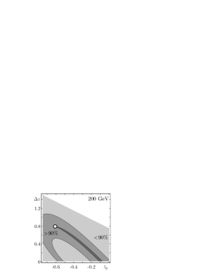
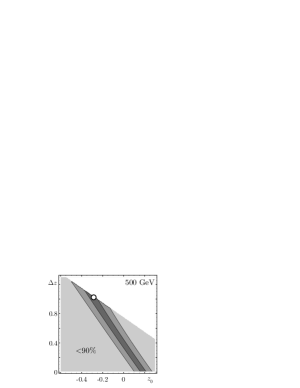
Figure 4: Relative contribution of the factor at $\bar{v}^{2}$ to the observable $\sigma_{V}$ as the function of the left boundary of the angle interval, $z_{0}$, and the interval length, $\Delta z$, at the center-of-mass energy 200 and 500 GeV. The shaded areas correspond to the contributions $>95\%$ (dark), from 90% to 95% (midtone), and $<90\%$ (light).

The relative contribution of the factor at $\bar{v}^{2}$ is defined as

$$\kappa_{V}=\frac{\Delta z}{\Delta z+\left|\int_{z_{0}}^{z_{0}+\Delta z}F_{a}\,dz\right|+\left|\int_{z_{0}}^{z_{0}+\Delta z}F_{av}\,dz\right|}$$ (30)

and shown in Fig. 4 as the function of the left boundary of the angle interval, $z_{0}$, and the interval length, $\Delta z$. In each plot the dark area corresponds to the observables which values are determined by the vector-vector coupling $\bar{v}^{2}$ with the accuracy $>95\%$. The area reflects the correlation of the width of the integration interval $\Delta z$ with the choice of the initial $z_{0}$ following from the mentioned requirements. Within this area we choose the observable which includes the largest number of bins (largest $\Delta z$). The corresponding values of $z_{0}$ and $\Delta z$ are marked by the white dot on the plots in Fig. 4. As the carried out analysis showed, the point $z_{0}$ is shifted to the right with increase in energy whereas $\Delta z$ remains approximately the same.

From the plots it follows that the most efficient intervals are

$$-0.6<z<0.2,\quad\sqrt{s}=200\mbox{ GeV},$$

$$-0.3<z<0.7,\quad\sqrt{s}=500\mbox{ GeV}.$$ (31)

Therefore the observable (29) allows to measure the $Z^{\prime}$ coupling to the electron vector current $\bar{v}^{2}$ with the efficiency $>95\%$.

Fitting the LEP2 final data with the one-parameter observable, we find the values of the $Z^{\prime}$ coupling to the electron vector current together with their 1$\sigma$ uncertainties:

$$\mathrm{ALEPH}: \bar{v}_{e}^{2}= -0.11\pm 6.53\times 10^{-4}$$

$$\mathrm{DELPHI}: \bar{v}_{e}^{2}= 1.60\pm 1.46\times 10^{-4}$$

$$\mathrm{L3}: \bar{v}_{e}^{2}= 5.42\pm 3.72\times 10^{-4}$$

$$\mathrm{OPAL}: \bar{v}_{e}^{2}= 2.42\pm 1.27\times 10^{-4}$$

$$\mathrm{Combined}: \bar{v}_{e}^{2}= 2.24\pm 0.92\times 10^{-4}.$$

As one can see, the most precise data of DELPHI and OPAL collaborations are resulted in the Abelian $Z^{\prime}$ hints at one and two standard deviation level, correspondingly. The combined value shows the 2$\sigma$ hint which corresponds to $0.006\leq|\bar{v}_{e}|\leq 0.020$.

4.4 Observables to pick out $\bar{a}^{2}$

In order to pick the axial-vector coupling $\bar{a}^{2}$ one needs to eliminate the dominant contribution coming from $\bar{v}^{2}$. Since the factor at $\bar{v}^{2}$ in the $d\tilde{\sigma}/dz$ equals unity, this can be done by summing up equal number of bins with positive and negative weights. In particular, the forward-backward normalized deviation of the differential cross-section appears to be sensitive mainly to $\bar{a}^{2}$,

$$\tilde{\sigma}_{\rm FB} = \int\nolimits_{0}^{z_{\rm max}}dz\,\frac{d\tilde{\sigma}}{dz}-\int\nolimits_{-z_{\rm max}}^{0}dz\,\frac{d\tilde{\sigma}}{dz}\tilde{F}_{a,\rm FB}\bar{a}^{2}+\tilde{F}_{av,\rm FB}\bar{a}\bar{v}.$$ (32)

The value $z_{\rm max}$ is determined by the number of bins included and, in fact, depends on the data set considered. The LEP2 experiment accepted $e^{+}e^{-}$ events with $|z|<0.72$. In what follows we take the angular cut $z_{\mathrm{max}}=0.7$ for definiteness.

The efficiency of the observable is determined as:

$$\kappa=\frac{|\tilde{F}_{a,\rm FB}|}{|\tilde{F}_{a,\rm FB}|+|\tilde{F}_{av,\rm FB}|}.$$ (33)

It can be estimated as $\kappa=0.9028$ for the center-of-mass energy 200 GeV and $\kappa=0.9587$ for 500 GeV. Thus, the observable

$$\tilde{\sigma}_{\rm FB}=0.224\bar{a}^{2}-0.024\bar{a}\bar{v},\quad\sqrt{s}=200\mbox{ GeV},$$

$$\tilde{\sigma}_{\rm FB}=0.472\bar{a}^{2}-0.020\bar{a}\bar{v},\quad\sqrt{s}=500\mbox{ GeV}$$ (34)

is mainly sensitive to the $Z^{\prime}$ coupling to the axial-vector current $\bar{a}^{2}$.

Consider a usual situation when experiment is not able to recognize the angular dependence of the differential cross-section deviation from its SM value with the proper accuracy because of loss of statistics. Nevertheless, a unique signal of the Abelian $Z^{\prime}$ boson can be determined. For this purpose the observables $\int_{z_{0}}^{z_{0}+\Delta z}(d\tilde{\sigma}/dz)dz$ and $\tilde{\sigma}_{\rm FB}$ must be measured. Actually, they are derived from the normalized deviation of the differential cross-section. If the deviation is inspired by the Abelian $Z^{\prime}$ boson both the observables are to be positive quantities simultaneously. This feature serves as the distinguishable signal of the Abelian $Z^{\prime}$ virtual state in the Bhabha process for the LEP2 energies as well as for the energies of future electron-positron collider ILC ($\geq 500$ GeV). The observables fix the unknown low energy vector and axial-vector $Z^{\prime}$ couplings to the electron current. Their values have to be correlated with the bounds on $\bar{a}^{2}$ and $\bar{v}^{2}$ derived by means of independent fits for other scattering processes.

We estimated the observable (4.4) related to the value of $\bar{a}^{2}$. Since in the Bhabha process the effects of the axial-vector coupling are suppressed with respect to those of the vector coupling, we expect much larger experimental uncertainties for $\bar{a}^{2}$. Indeed, the LEP2 data lead to the huge errors for $\bar{a}^{2}$ of order $10^{-3}-10^{-4}$. The mean values are negative numbers which are too large to be interpreted as a manifestation of some heavy virtual state beyond the energy scale of the SM.

Thus, the LEP2 data constrain the value of $\bar{v}^{2}$ at the $2\sigma$ CL which could correspond to the Abelian $Z^{\prime}$ boson with the mass of the order 1 TeV. In contrast, the value of $\bar{a}^{2}$ is a large negative number with a significant experimental uncertainty. This can not be interpreted as a manifestation of some heavy virtual state beyond the energy scale of the SM.

4.5 Many-parameter fits

To account for all the accessible data of LEP experiments, we address to many parameter fits [17]. As the basic observable to fit the LEP2 experiment data on the Bhabha process we propose the differential cross-section

$$\left.\frac{d\sigma^{\mathrm{Bhabha}}}{dz}-\frac{d\sigma^{\mathrm{Bhabha},SM}}{dz}\right|_{z=z_{i},\sqrt{s}=\sqrt{s_{i}}},$$ (35)

where $i$ runs over the bins at various center-of-mass energies $\sqrt{s}$. The final differential cross-sections measured by the ALEPH [22] (130-183 GeV), DELPHI [5] (189-207 GeV), L3 [23] (183-189 GeV), and OPAL [2, 3, 4] (130-207 GeV) collaborations are taken into consideration (299 bins).

As the observables for $e^{+}e^{-}\to\mu^{+}\mu^{-},\tau^{+}\tau^{-}$ processes, we consider the total cross-section and the forward-backward asymmetry

$$\sigma^{\ell^{+}\ell^{-}}_{T}-\sigma_{T}^{\ell^{+}\ell^{-},\mathrm{SM}},\quad\left.A^{\ell^{+}\ell^{-}}_{FB}-A_{FB}^{\ell^{+}\ell^{-},\mathrm{SM}}\right|_{\sqrt{s}=\sqrt{s_{i}}},$$ (36)

where $i$ runs over 12 center-of-mass energies $\sqrt{s}$ from 130 to 207 GeV. We consider the combined LEP2 data [1] for these observables (24 data entries for each process). These data are more precise as the corresponding differential cross-sections. Our analysis is based on the fact that the kinematics of $s$-channel processes is rather simple and the differential cross-section is effectively a two-parametric function of the scattering angle. The total cross-section and the forward-backward asymmetry incorporate complete information about the kinematics of the process and therefore are an adequate alternative for the differential cross-sections.

The data are analysed by means of the $\chi^{2}$ fit [17]. Denoting the observables (35)–(36) by $\sigma_{i}$, one can construct the $\chi^{2}$-function,

$$\chi^{2}(\bar{a},\bar{v}_{e},\bar{v}_{\mu},\bar{v}_{\tau})=\sum\limits_{i}\left[\frac{\sigma^{\mathrm{ex}}_{i}-\sigma^{\mathrm{th}}_{i}(\bar{a},\bar{v}_{e},\bar{v}_{\mu},\bar{v}_{\tau})}{\delta\sigma_{i}}\right]^{2},$$ (37)

where $\sigma^{\mathrm{ex}}$ and $\delta\sigma$ are the experimental values and the uncertainties of the observables, and $\sigma^{\mathrm{th}}$ are their theoretical expressions presented in Eqs. (26)–(27). The sum in Eq. (37) refers to either the data for one specific process or the combined data for several processes. By minimizing the $\chi^{2}$-function, the maximal-likelihood estimate for the $Z^{\prime}$ couplings can be derived. The $\chi^{2}$-function is also used to plot the confidence area in the space of parameters $\bar{a}$, $\bar{v}_{e}$, $\bar{v}_{\mu}$, and $\bar{v}_{\tau}$. Note that in this way of experimental data treating all the possible correlations are neglected. We believe that at the present stage of investigation this is reasonable, because the Collaborations have never reported on this possibility.

For all the considered processes, the theoretic predictions $\sigma^{\mathrm{th}}_{i}$ are linear combinations of products of two $Z^{\prime}$ couplings

$$\sigma^{\mathrm{th}}_{i}=\sum_{j=1}^{7}C_{ij}A_{j},\qquad A_{j}=\{\bar{a}^{2},\bar{v}_{e}^{2},\bar{a}\bar{v}_{e},\bar{v}_{e}\bar{v}_{\mu},\bar{v}_{e}\bar{v}_{\tau},\bar{a}\bar{v}_{\mu},\bar{a}\bar{v}_{\tau}\},$$

where $C_{ij}$ are known numbers.

In the Bhabha process, the $Z^{\prime}$ effects are determined by three linear-independent contributions coming from $\bar{a}^{2}$, $\bar{v}_{e}^{2}$, and $\bar{a}\bar{v}_{e}$ and the number degrees of freedom (d.o.f) $M=3$. As for the $e^{+}e^{-}\to\mu^{+}\mu^{-},\tau^{+}\tau^{-}$ processes, the observables depend on four linear-independent terms for each process: $\bar{a}^{2}$, $\bar{v}_{e}\bar{v}_{\mu}$, $\bar{v}_{e}\bar{a}$, $\bar{a}\bar{v}_{\mu}$ for $e^{+}e^{-}\to\mu^{+}\mu^{-}$; and $\bar{a}^{2}$, $\bar{v}_{e}\bar{v}_{\tau}$, $\bar{v}_{e}\bar{a}$, $\bar{a}\bar{v}_{\tau}$ for $e^{+}e^{-}\to\tau^{+}\tau^{-}$ ($M=4$). Note that some terms in the observables for different processes are the same. Therefore, the number of $\chi^{2}$ d.o.f. in the combined fits is less than the sum of d.o.f. for separate processes. Hence, the predictive power of the larger set of data is not drastically spoiled by the increased number of d.o.f. In fact, combining the data of the Bhabha and $e^{+}e^{-}\to\mu^{+}\mu^{-}$ ($\tau^{+}\tau^{-}$) processes together we have to treat five linear-independent terms. The complete data set for all the lepton processes is ruled by seven d.o.f. As a consequence, the combination of the data for all the lepton processes is possible.

The parametric space of couplings ($\bar{a}$, $\bar{v}_{e}$, $\bar{v}_{\mu}$, $\bar{v}_{\tau}$) is four-dimensional. However, for the Bhabha process it is reduced to the plane ($\bar{a}$, $\bar{v}_{e}$), and to the three-dimensional volumes ($\bar{a}$, $\bar{v}_{e}$, $\bar{v}_{\mu}$), ($\bar{a}$, $\bar{v}_{e}$, $\bar{v}_{\tau}$) for the $e^{+}e^{-}\to\mu^{+}\mu^{-}$ and $e^{+}e^{-}\to\tau^{+}\tau^{-}$ processes, correspondingly. The predictive power of data is distributed not uniformly over the parameters. The parameters $\bar{a}$ and $\bar{v}_{e}$ are present in all the considered processes and appear to be significantly constrained. The couplings $\bar{v}_{\mu}$ or $\bar{v}_{\tau}$ enter when the processes $e^{+}e^{-}\to\mu^{+}\mu^{-}$ or $e^{+}e^{-}\to\tau^{+}\tau^{-}$ are accounted for. So, in these processes, we also study the projection of the confidence area onto the plane ($\bar{a},\bar{v}_{e}$).

The origin of the parametric space, $\bar{a}=\bar{v}_{e}=0$, corresponds to the absence of the $Z^{\prime}$ signal. This is the SM value of the observables. This point could occur inside or outside of the confidence area at a fixed CL. When it lays out of the confidence area, this means the distinct signal of the Abelian $Z^{\prime}$. Then the signal probability can be defined as the probability that the data agree with the Abelian $Z^{\prime}$ boson existence and exclude the SM value. This probability corresponds to the most stringent CL (the largest $\chi^{2}_{\mathrm{CL}}$) at which the point $\bar{a}=\bar{v}_{e}=0$ is excluded. If the SM value is inside the confidence area, the $Z^{\prime}$ boson is indistinguishable from the SM. In this case, upper bounds on the $Z^{\prime}$ couplings can be determined.

The 95% CL areas in the ($\bar{a},\bar{v}_{e}$) plane for the separate processes are plotted in Fig. 6. As it is seen, the Bhabha process constrains both the axial-vector and vector couplings. As for the $e^{+}e^{-}\to\mu^{+}\mu^{-}$ and $e^{+}e^{-}\to\tau^{+}\tau^{-}$ processes, the axial-vector coupling is significantly constrained, only. The confidence areas include the SM point at the meaningful CLs, so the experiment could not pick out clearly the Abelian $Z^{\prime}$ signal from the SM. An important conclusion from these plots is that the experiment significantly constrains only the couplings entering sign-definite terms in the cross-sections.

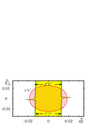
Figure 5: The 95% CL areas in the ($\bar{a},\bar{v}_{e}$) plane for the Bhabha, $e^{+}e^{-}\to\mu^{+}\mu^{-}$, and $e^{+}e^{-}\to\tau^{+}\tau^{-}$ processes.

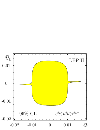
Figure 6: The projection of the 95% CL area onto the ($\bar{a},\bar{v}_{e}$) plane for the combination of the Bhabha, $e^{+}e^{-}\to\mu^{+}\mu^{-}$, and $e^{+}e^{-}\to\tau^{+}\tau^{-}$ processes.

The combination of all the lepton processes is presented in Fig. 6. There is no visible signal beyond the SM. The couplings to the vector and axial-vector electron currents are constrained by the many-parameter fit as $|\bar{v}_{e}|<0.013$, $|\bar{a}|<0.019$ at the 95% CL. If the charge corresponding to the $Z^{\prime}$ interactions is assumed to be of order of the electromagnetic one, then the $Z^{\prime}$ mass should be greater than 0.67 TeV. For the charge of order of the SM $SU(2)_{L}$ coupling constant $m_{Z^{\prime}}\geq 1.4$ TeV. One can see that the constraint is not too severe to exclude the $Z^{\prime}$ searches at the LHC.

Let us compare the obtained results with the one-parameter fits. As one can see, the most precise data of DELPHI and OPAL collaborations are resulted in the Abelian $Z^{\prime}$ hints at one and two standard deviation level, correspondingly. The combined value shows the 2$\sigma$ hint, which corresponds to $0.006\leq|\bar{v}_{e}|\leq 0.020$. On the other hand, our many-parameter fit constrains the $Z^{\prime}$ coupling to the electron vector current as $|\bar{v}_{e}|\leq 0.013$ with no evident signal. Why does the one-parameter fit of the Bhabha process show the 2$\sigma$ CL hint whereas there is no signal in the two-parameter one? Our one-parameter observable accounts mainly for the backward bins. This is in accordance with the kinematic features of the process: the backward bins depend mainly on the vector coupling $\bar{v}^{2}_{e}$, whereas the contributions of other couplings are kinematically suppressed (see Fig. 2). Therefore, the difference of the results can be inspired by the data sets used. To clarify this point, we perform the many-parameter fit with the 113 backward bins ($z\leq 0$), only. The $\chi^{2}$ minimum, $\chi^{2}_{\mathrm{min}}=93.0$, is found in the non-zero point $|\bar{a}|=0.0005$, $\bar{v}_{e}=0.015$. This value of the $Z^{\prime}$ coupling $\bar{v}_{e}$ is in an excellent agreement with the mean value obtained in the one-parameter fit. The 68% confidence area in the ($\bar{a},\bar{v}_{e}$) plane is plotted in Fig. 7. There is a visible hint of the Abelian $Z^{\prime}$ boson. The zero point $\bar{a}=\bar{v}_{e}=0$ (the absence of the $Z^{\prime}$ boson) corresponds to $\chi^{2}=97.7$. It is covered by the confidence area with $1.3\sigma$ CL. Thus, the backward bins show the $1.3\sigma$ hint of the Abelian $Z^{\prime}$ boson in the many-parameter fit. So, the many-parameter fit is less precise than the analysis of the one-parameter observables.

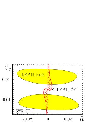
Figure 7: The 68% CL area in the ($\bar{a},\bar{v}_{e}$) plane from the backward bins of the Bhabha process in the LEP2 experiments (the shaded area). The hatched area is the 68% CL area from the LEP 1 data on the Bhabha process.

Table 4: The summary of the fits of the LEP data for the dimensionless contact couplings (6).

Data	$\bar{v}^{2}_{e}$, $\times 10^{-4}$	$\bar{a}^{2}$, $\times 10^{-5}$
LEP1
$e^{-}e^{+}$, 68% CL	-	$1.25\pm 1.25$
LEP2, one-parameter fits
$e^{-}e^{+}$, 68% CL	$2.24\pm 0.92$	-
$\mu\mu$, 68% CL	-	$3.66^{+4.89}_{-4.86}$
$\mu\mu$,$\tau\tau$, 68% CL	-	$1.33^{+3.89}_{-3.87}$
LEP2, many-parameter fits
$e^{-}e^{+},\mu\mu,\tau\tau$, 95% CL	$\leq 1.69$	$\leq 36.1$
$e^{-}e^{+}$ backward, 68% CL	$2.25^{+1.79}_{-2.07}$	$\leq 94.9$

At LEP1 experiments [26] the $Z$-boson couplings to the vector and axial-vector lepton currents ($g_{V}$, $g_{A}$) were precisely measured. The Bhabha process shows the 1$\sigma$ deviation from the SM values for Higgs boson masses $m_{H}\geq 114$ GeV (see Fig. 7.3 of Ref. [26]). This deviation could be considered as the effect of the $Z$–$Z^{\prime}$ mixing. It is interesting to estimate the bounds on the $Z^{\prime}$ couplings following from these experiments.

Due to relations (8), the $Z$–$Z^{\prime}$ mixing angle is completely determined by the axial-vector coupling $\bar{a}$. So, the deviations of $g_{V}$, $g_{A}$ from their SM values are governed by the couplings $\bar{a}$ and $\bar{v}_{e}$,

$$g_{V}-g_{V}^{\mathrm{SM}}=-49.06\bar{a}\bar{v}_{e},\quad g_{A}-g_{A}^{\mathrm{SM}}=49.06\bar{a}^{2}.$$ (38)

Let us assume that the total deviation of theory from experiments follows due to the $Z$–$Z^{\prime}$ mixing. This gives an upper bound on the $Z^{\prime}$ couplings. In this way one can estimate whether the $Z^{\prime}$ boson is excluded by the experiments or not.

The 1$\sigma$ CL area for the Bhabha process from Ref. [26] is converted into the ($\bar{a},\bar{v}_{e}$) plane in Fig. 7. The SM values of the couplings correspond to the top quark mass $m_{t}=178$ GeV and the Higgs scalar mass $m_{H}=114$ GeV. As it is seen, the LEP1 data on the Bhabha process is compatible with the Abelian $Z^{\prime}$ existence at the $1\sigma$ CL. The axial-vector coupling is constrained as $|\bar{a}|\leq 0.005$. This bound corresponds to $\bar{a}^{2}\leq 2.5\times 10^{-5}$, which agrees with the one-parameter fits of the LEP2 data for $e^{+}e^{-}\to\mu^{+}\mu^{-},\tau^{+}\tau^{-}$ processes ($\bar{a}^{2}=1.3\pm 3.89\times 10^{-5}$ at 68% CL). On the other hand, the vector coupling constant $\bar{v}_{e}$ is practically unconstrained by the LEP1 experiments.

For the convenience, in Table 4 we collect the summary of the fits of the LEP data in terms of dimensionless contact couplings (6). From the analysis carried out we come to conclusion that, in principle, the LEP experiments were able to detect the $Z^{\prime}$-boson signals if the statistics had been sufficient.

5 Model independent results and search for $Z^{\prime}$ at the LHC

In this section we discuss all the assumptions giving a possibility to pick out the $Z^{\prime}$ signal and determine its characteristics in a model independent way. We also note the role of the present results for the LHC and future ILC experiments.

As it was already noted, in searching for this particle at the LEP and Tevatron a model dependent analysis was applied. As the main motivation for this approach it was the different number of chiral fermions involved in different models (see, for example, Ref. [7]). In this way the low bounds on $m_{Z^{\prime}}$ have been estimated and the smallness of the $Z$–$Z^{\prime}$ mixing was also observed.

On the contrary, in our approach the relations (7) between the parameters of the effective low energy Lagrangians have been accounted for that gave a possibility to determine not only the bounds but also the mass and other parameters of the $Z^{\prime}$.

To be precise, let us note all the assumptions used in our investigations. We analyzed the four-fermion scattering amplitudes of order $\sim m_{Z^{\prime}}^{-2}$ generated by the $Z^{\prime}$ virtual states. The vertices linear in $Z^{\prime}$ were included into the effective low-energy Lagrangian. We also impose a number of natural conditions. The interactions of a renormalizable type are dominant at low energies $\sim m_{W}$. The non-renormalizable interactions generated at high energies due to radiation corrections are suppressed by the inverse heavy mass $\sim 1/m_{Z^{\prime}}$ and neglected. We also assumed that the $SU(2)_{L}\times U(1)_{Y}$ gauge group of the SM is a subgroup of the GUT group. As a consequence, all the structure constants connecting two SM gauge bosons with $Z^{\prime}$ have to be zero. Hence, the interactions of gauge fields of the types $Z^{\prime}W^{+}W^{-},Z^{\prime}ZZ$, and other are absent at a tree level. Our effective Lagrangian is also consistent with the absence of the tree-level flavor-changing neutral currents (FCNCs) in the fermion sector. The renormalizable interactions of fermions and scalars are described by the Yukawa Lagrangian that accounts for different possibilities of the Yukawa sector without the tree-level FCNCs. These assumptions are quite general and satisfied in a wide class of $E_{6}$ inspired models.

Within these constraints for the low energy effective Lagrangian the relations (7),(8) have been derived. Correspondingly, the model independent estimates of the mass $m_{Z^{\prime}}$ and other parameters are regulated by the noted requirements. Therefore, the extended underlying model has also to accept them.

In this regard, let us discuss the role of the obtained estimates for the LHC. As it is well known (see, for example, [7, 8]), there are many tools at the LHC for $Z^{\prime}$ identification. But many of them are only applicable if this particle is relatively light. Our results are in favor to this case.

Next important point is the determination of $Z^{\prime}$ couplings to the various SM fermions. As we have shown, the axial-vector couplings of the $Z^{\prime}$ to the SM fermions are universal and proportional to its coupling to the Higgs field. Hence we have obtained an estimate of the $a=a_{f}$ couplings for both leptons and quarks. This is an essential input because experimental analysis for the LHC have mainly concentrated on being able to distinguish models and not on actual couplings. The vector coupling $v_{e}$ was also estimated that, in particular, may help to distinguish the decay of the $Z^{\prime}$ resonance state to $e^{+}e^{-}$ pairs. Since the couplings $a_{e}$ and $v_{e}$ were estimated there is a possibility to distinguish this process from the decay of the $KK$ system. In the literature on searching for the $Z^{\prime}$ it is also mentioned [8, 27] that the determination of the $Z^{\prime}$ couplings to fermions could be fulfilled channel by channel, $a_{e},v_{e},v_{e,b},a_{e,b}$, …. In that considerations the relations between the parameters have not been taken into account. But this is very essential for treating of experimental data and introducing the relevant observables to measure. Our consideration could be useful in this problem.

Other parameter is the $Z$–$Z^{\prime}$ mixing which is responsible for the different decay processes and the effective interaction vertices generated at the LHC [7, 8]. It is also determined by the axial-vector coupling (see Eq. (8)) and estimated in a model independent way. Remind that in our analysis the mixing was systematically accounted for. Its value is of the same order of magnitude as the parameters that were fitted in experiments. It worth to note also that the existence of other heavy particles with masses $m_{X}\geq m_{Z^{\prime}}$ does not influence the RG relations.

An important role of the model independent results for searching for $Z^{\prime}$ at the Tevatron, LHC and ILC consists, in particular, in a possibility to determine the particle as a virtual state due to a large amount of relevant events. We mentioned already that, in principle, LEP2 experiments were able to determine it if the statistics was sufficiently large. Experiments at the ILC will increase in many times the data set of interest. In fact, the observables, introduced in sects. 6 and 7 for picking out uniquely $a_{f}^{2}$ and $v_{e}^{2}$ couplings in the leptonic scattering process, are also effective at energies $\sqrt{s}\geq 500$ GeV and could be applied in future experiments at ILC.

Other model independent methods of searching for the $Z^{\prime}$ as a resonance state are proposed in the literature (see Refs. [27, 28, 29]). We do not discuss them here because they take into consideration no relations between the parameters. As we mentioned already, the main goal of the present paper is to adduce model independent information about the $Z^{\prime}$ followed from experiments at low energies. Different aspects of $Z^{\prime}$ physics at the LHC are out of the scope of it.

6 Discussion

In this section we collect in a convenient form all the results obtained and make a comparison with other investigations on searching for $Z^{\prime}$ at low energies. In fact, this is a large area to discuss. References to numerous results obtained in either model dependent or model independent approaches can be found in Refs. [7, 8]. Further subdivision can be done into the considerations accounting for any type correlations between the parameters of the low energy effective interactions and that of assuming complete independence of them. Because of a large amount of fitting parameters the latter are less predictable.

Now, for a convenience of readers we present the results of fits of the $Z^{\prime}$ parameters in terms of the popular notations [6, 7]. The Lagrangian reads

$${\cal L}_{Z\bar{f}f} = \frac{1}{2}Z_{\mu}\bar{f}\gamma^{\mu}\left[(v^{\mathrm{SM}}_{f}+\Delta^{V}_{f})-\gamma^{5}(a^{\mathrm{SM}}_{f}+\Delta^{A}_{f})\right]f,$$

$${\cal L}_{Z^{\prime}\bar{f}f} = \frac{1}{2}Z^{\prime}_{\mu}\bar{f}\gamma^{\mu}\left[(v^{\prime}_{f}-\gamma^{5}a^{\prime}_{f})\right]f,$$ (39)

with the SM values of the $Z$ couplings

$$v^{\mathrm{SM}}_{f}=\frac{e\left(T_{3f}-2Q_{f}\sin^{2}\theta_{W}\right)}{\sin\theta_{W}\cos\theta_{W}},\qquad a^{\mathrm{SM}}_{f}=\frac{e\,T_{3f}}{\sin\theta_{W}\cos\theta_{W}},$$

where $e$ is the positron charge, $Q_{f}$ is the fermion charge in the units of $e$, $T_{3f}=1/2$ for the neutrinos and $u$-type quarks, and $T_{3f}=-1/2$ for the charged leptons and $d$-type quarks.

Table 5: The summary of the fits of the LEP data for the maximum likelihood values of the $Z^{\prime}$ couplings (6) to the SM fermions and of the $Z$–$Z^{\prime}$ mixing angle $\theta_{0}$. $M=\frac{m_{Z^{\prime}}}{1\,\mathrm{TeV}}$ denotes the unknown value of the $Z^{\prime}$ mass in TeV units.

Data	$|\theta_{0}|$, $\times 10^{-3}$	$|v^{\prime}_{e}|$, $\times 10^{-1}$	$|a^{\prime}_{f}|$, $\times 10^{-1}$	$\Delta^{A}_{e}$, $\times 10^{-3}$
LEP1
$e^{-}e^{+}$	${3.17}{M}^{-1}$	-	$1.38M$	0.437
LEP2, one-parameter fits
$e^{-}e^{+}$	-	$5.83M$	-	-
$\mu^{-}\mu^{+}$	$5.42{M}^{-1}$	-	$2.36M$	1.278
$\mu^{-}\mu^{+},\tau^{-}\tau^{+}$	$3.27{M}^{-1}$	-	$1.42M$	0.464
LEP2, many-parameter fits
$e^{-}e^{+}$, $z<0$	-	$5.84M$	-	-

Table 6: The summary of the fits of the LEP data for the confidence intervals for the $Z^{\prime}$ couplings (6) to the SM fermions and for the $Z$–$Z^{\prime}$ mixing angle $\theta_{0}$. $M=\frac{m_{Z^{\prime}}}{1\,\mathrm{TeV}}$ denotes the unknown value of the $Z^{\prime}$ mass in TeV units.

Data	CL	$|\theta_{0}|$, $\times 10^{-3}$	$|v^{\prime}_{e}|$, $\times 10^{-1}$	$|a^{\prime}_{f}|$, $\times 10^{-1}$	$\Delta^{A}_{e}$, $\times 10^{-3}$
LEP1
$e^{-}e^{+}$	68%	$(0;4.48){M}^{-1}$	-	$(0;1.95)M$	$(0;0.873)$
LEP2, one-parameter fits
$e^{-}e^{+}$	95%	-	$(2.46;7.87)M$	-	-
$\mu^{-}\mu^{+}$	95%	$(0;10.39){M}^{-1}$	-	$(0;4.52)M$	$(0;4.694)$
$\mu^{-}\mu^{+}$, $\tau^{-}\tau^{+}$	95%	$(0;8.64){M}^{-1}$	-	$(0;3.75)M$	$(0;3.244)$
LEP2, many-parameter fits
$e^{-}e^{+}$, $\mu^{-}\mu^{+}$, $\tau^{-}\tau^{+}$	95%	$(0;17.03){M}^{-1}$	$(0;5.06)M$	$(0;7.40)M$	$(0;12.607)$
$e^{-}e^{+}$, $z<0$	68%	$(0;27.61){M}^{-1}$	$(1.68;7.83)M$	$(0;12.00)M$	$(0;33.1288)$

The results of fits of the $Z^{\prime}$ couplings to the SM leptons obtained from the analysis of LEP experiments are adduced in the Tables 5-6. Remind that due to the universality of the axial-vector coupling $a_{f}$ the same estimates also hold for quarks. First of all, one parameter fits of LEP experiments as well as the many-parameter fit for the $e^{+}e^{-}$ backward bins show the hints of the $Z^{\prime}$ boson at the 1-2$\sigma$ CL. Due to this fact, the fits allow to determine the maximum likelihood values of $Z^{\prime}$ parameters. In spite of uncertainties, these values can be used as a guiding line for the estimation of possible $Z^{\prime}$ effects in the Tevatron and LHC experiments. The maximum likelihood values are given in Table 5. As it is seen, different fits obtained for different processes lead to the comparable values of the $Z^{\prime}$ parameters.

In Table 6 we present the confidence intervals for the fitted parameters. It gives a possibility to estimate the uncertainty of the $Z^{\prime}$ couplings as well as the lower bounds on the parameters. The results of fits are also shown in Figs. 8-9. To summarize them we note that the data of the LEP2 experiments are compatible at 1-2 $\sigma$ level with the existence of the not heavy $Z^{\prime}$ boson.

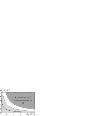
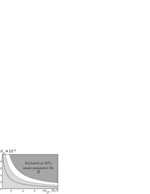
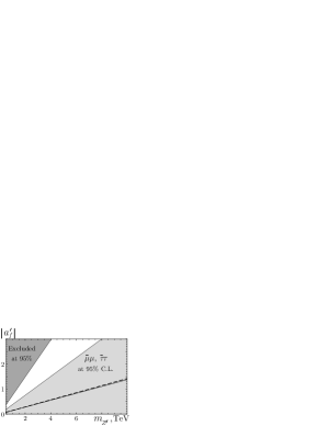
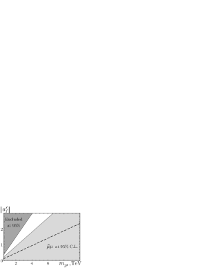
Figure 8: The maximum likelihood values and the confidence intervals for the $Z$–$Z^{\prime}$ mixing angle ($\theta_{0}$) and the axial-vector couplings to the SM fermions ($a^{\prime}_{f}$) by the LEP 2 data. The values excluded at 95% CL by the many-parameter fit of $e^{+}e^{-}\to l^{+}l^{-}$ are shown in dark gray. The results of fits based on the one-parameter observables are shown in light gray for $e^{+}e^{-}\to\mu^{+}\mu^{-},\tau^{+}\tau^{-}$ (left) and for $e^{+}e^{-}\to\mu^{+}\mu^{-}$ (right). The maximum likelihood value are plotted as the dashed lines. The dotted lines correspond to the maximum likelihood values obtained from the LEP1 data.

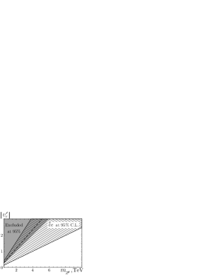
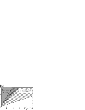
Figure 9: The maximum likelihood values and the confidence intervals for the vector coupling to electron current ($v^{\prime}_{e}$) by the LEP 2 data. The values excluded at 95% CL by the many-parameter fit of $e^{+}e^{-}\to l^{+}l^{-}$ are shown in dark gray. The left panel represents the results of fits based on the one-parameter observable for $e^{+}e^{-}\to e^{+}e^{-}$. The right panel shows the 1$\sigma$ CL area for the many-parameter fit of backward bins of $e^{+}e^{-}\to e^{+}e^{-}$. The maximum likelihood value are plotted as the dashed lines.

Now we compare the above results with the ones of other fits accounting for the $Z^{\prime}$ presence. As it was mentioned in Introduction, LEP collaborations have determined the model dependent low bounds on the $Z^{\prime}$ mass which vary in a wide energy interval dependently on a model. The same has also been done for Tevatron experiments. The modern low bound is $m_{Z^{\prime}}\geq 850$ GeV. It is also well known that though almost all the present day data are described by the SM [1, 2, 3, 4, 5, 26], the overall fit to the standard model is not very good. In Ref. [9] it was showed that the large difference in $\sin^{2}\theta^{\mathrm{lept}}_{\mathrm{eff}}$ from the forward-backward asymmetry $A^{b}_{fb}$ of the bottom quarks and the measurements from the SLAC SLD experiment can be explained for physically reasonable Higgs boson mass if one allows for one or more extra $U(1)$ fields, that is $Z^{\prime}$. A specific model to describe $Z^{\prime}$ physics of interest was proposed which introduces two type couplings to the hyper charge $Y$ and to the baryon-minus-lepton number $B-L$. Within this model by using a number of precision measurements from LEP1, LEP2, SLD and Tevatron experiments the parameters $a_{Y}$ and $a_{B-L}$ of the model were fitted. The presence of $Z^{\prime}$ was not excluded at 68% CL. The value of $a_{Y}$ was estimated to be of the same order of magnitude as in our analysis and is comparable with values of other parameters detected in the LEP experiments. The erroneous claim that $a_{Y}$ is two order less then the value derived from our Table 4 is, probably, a consequence of some missed factors. The upper limit on the mass was also obtained $m_{Z^{\prime}}\leq 2.6$ TeV .

These two analyzes are different but complementary. A common feature of them is an accounting for the $Z^{\prime}$ gauge boson as a necessary element of the data fits. The results are in accordance at 68-95% CL with the existence of the $Z^{\prime}$ which has a good chance to be discovered at Tevatron and/or LHC.

References

- [1] J. Alcaraz et al. , hep-ex/0612034 (2006).
- [2] OPAL Collab. (G. Abbiendi et al.), Eur. Phys. J. C 33, 173 (2004).
- [3] OPAL Collab. (G. Abbiendi et al.), Eur. Phys. J. C 6, 1 (1999).
- [4] OPAL Collab. (K. Ackerstaff et al.), Eur. Phys. J. C 2, 441 (1998).
- [5] DEPHI COllab. (J. Abdallah et al.), Eur. Phys. J. C 45, 589 (2006).
- [6] A. Leike, Phys. Rept. 317, 143 (1999).
- [7] P. Langacker , arXiv:0801.1345 (2008).
- [8] T. G. Rizzo , hep-ph/0610104 (2006).
- [9] A. Ferroglia, A. Lorca and J. J. van der Bij, Annalen Phys. 16, 563 (2007).
- [10] J. Erler, P. Langacker, S. Munir and E. R. Pena, JHEP 08, 017 (2009).
- [11] F. del Aguila, J. de Blas and M. Perez-Victoria , arXiv:1005.3998 (2010).
- [12] A. V. Gulov and V. V. Skalozub, Eur. Phys. J. C 17, 685 (2000).
- [13] A. V. Gulov and V. V. Skalozub, Phys. Rev. D 61, 055007 (2000).
- [14] A. V. Gulov and V. V. Skalozub, int. J. Mod. Phys. A 16, 179 (2001).
- [15] V. I. Demchik, A. V. Gulov, V. V. Skalozub and A. Y. Tischenko, Phys. Atom. Nucl. 67, 1312 (2004).
- [16] A. V. Gulov and V. V. Skalozub, Phys. Rev. D 70, 115010 (2004).
- [17] A. V. Gulov and V. V. Skalozub, Phys. Rev. D 76, 075008 (2007).
- [18] J. L. Hewett and T. G. Rizzo, Phys. Rept. 183, 193 (1989).
- [19] M. Cvetic and B. W. Lynn, Phys. Rev. D 35, 51 (1987).
- [20] G. Degrassi and A. Sirlin, Phys. Rev. D 40, 3066 (1989).
- [21] T. G. Rizzo, Phys. Rev. D 55, 5483 (1997).
- [22] ALEPH Collab. (R. Barate et al.), Eur. Phys. J. C 12, 183 (2000).
- [23] L3 Collab. (M. Acciarri et al.), Phys. Lett. B 479, 101 (2000).
- [24] A. A. Babich et al., Eur. Phys. J. C 29, 103 (2003).
- [25] W. Eadie, D. Dryard, F. James, M. Roos and B. Sadoulet (eds.), Statistical Methods in Experimental Physics (North-Holland, Amsterdam, 1971).
- [26] ALEPH Collab., DELPHI Collab., L3 Collab., OPAL Collab., SLD Collab., LEP Electroweak Working Group, SLD Electroweak Group and SLD Heavy Flavour Group, Phys. Rept. 427, 257 (2006).
- [27] M. Dittmar, A. S. Nicollerat and A. Djouadi, Phys. Lett. B 583, 111 (2004).
- [28] C. Coriano, A. E. Faraggi and M. Guzzi, Phys. Rev. D 78, 015012 (2008).
- [29] F. Petriello and S. Quackenbush, Phys. Rev. D 77, 115004 (2008).