Message Error Analysis of Loopy Belief Propagation for the Sum-Product Algorithm

Abstract

Belief propagation is known to perform extremely well in many practical statistical inference and learning problems using graphical models, even in the presence of multiple loops. The iterative use of belief propagation algorithm on loopy graphs is referred to as Loopy Belief Propagation (LBP). Various sufficient conditions for convergence of LBP have been presented; however, general necessary conditions for its convergence to a unique fixed point remain unknown. Because the approximation of beliefs to true marginal probabilities has been shown to relate to the convergence of LBP, several methods have been explored whose aim is to obtain distance bounds on beliefs when LBP fails to converge. In this paper, we derive uniform and non-uniform error bounds on messages, which are tighter than existing ones in literature, and use these bounds to derive sufficient conditions for the convergence of LBP in terms of the sum-product algorithm. We subsequently use these bounds to study the dynamic behavior of the sum-product algorithm, and analyze the relation between convergence of LBP and sparsity and walk-summability of graphical models. We finally use the bounds derived to investigate the accuracy of LBP, as well as the scheduling priority in asynchronous LBP.

Keywords: Graphical Model, Bayesian Networks, Markov Random Fields, Loopy Belief Propagation, Error Analysis.

1 Introduction

Probabilistic inference for large-scale multivariate random variables is very expensive computationally. Belief propagation (BP) algorithms are designed to reduce the computational burden by exploiting the factorization of joint density functions captured by the topological structure of graphical models [Bishop (2006); Jordan (1999); Kschischang et al. (2001); Wainwright and Jordan (2008)]. BP is known to converge to the exact inference on acyclic graphs (i.e. trees) or graphs that contain a single loop. In the case of graphs with multiple loops, BP results in an iterative method referred to as loopy belief propagation (LBP). The use of LBP generally provides remarkably good approximations in real-world applications; e.g., turbo decoding and stereo matching [Mceliece et al. (1998); Sun et al. (2003)].

Because LBP does not always converge, sufficient conditions for its convergence have been extensively investigated in the past using various approaches [Tatikonda and Jordan (2002); Heskes (2004); Ihler et al. (2005); Mooij and Kappen (2007)]. Necessary conditions for convergence of LBP, however, remain unknown.  Tatikonda and Jordan (2002) related convergence of LBP to the uniqueness of a sequence of Gibbs measures defined on the associated computation tree. He subsequently developed a testable sufficient condition for convergence of LBP by applying Simon’s condition [Georgii (1988)].  Heskes (2004) presented sufficient conditions for uniqueness of fixed points in LBP by relying on the uniqueness of minima of the Bethe free energy. He related the strength of the potentials with the convergence of the LBP algorithm, which leads to better sufficient conditions than those exclusively relying on the structure of the graph.

Recently, several papers have investigated the message updating functions of the LBP algorithm as contractive mappings.  Ihler et al. (2005) analyzed the contractive dynamics of message-error propagation in belief networks using dynamic-range measure as a metric, and obtained error bounds and sufficient conditions for convergence of LBP message passing.  Mooij and Kappen (2007) derived sufficient conditions for convergence of LBP based on quotient norms of contractive mappings, which are invariant to scaling and shown to be valid for potential functions containing zeros.

For Gaussian graphical models, Malioutov et al. (2006) related the convergence of means and variances to walk sums and defined walk-summability with respect to spectral radius of partial correlation coefficient matrix. For binary graphs, Watanabe and Fukumizu (2009) presented an edge zeta function based on weighted prime cycles, and related convexity of Bethe free energy with the determinant formula of edge zeta function. They showed similar walk-summability of binary graphs by relating the spectra of correlation coefficient matrix with Hessian of Bethe free energy. For general graphical models, Mooij and Kappen (2007) derived certain interaction coefficients between random variables based on strength of potential functions, and related the spectral radius of coefficient matrix with the convergence of LBP. Enlightened by those similar analysis, we defined walk-summable for general graphs and compared walk-summability with other existing convergence conditions.

Although the beliefs may not be true marginal probabilities when the LBP algorithm converges, they have been shown to provide good approximations by Weiss (2000). When the LBP algorithm does not converge, however, beliefs are not good approximations of true marginals because the Bethe free energy does not provide a good approximation of the Gibbs-Helmholtz free energy [Yedidia et al. (2004)]. Exactness and accuracy of the LBP algorithm has consequently gained interest in recent years.  Tatikonda (2003) derived bounds on exact marginals by relying on the girth of the graph (i.e. the number of edges in the shortest cycle in the graph) and the properties of Dobrushin’s interdependence matrix [Salas and Sokal (1997)].  Taga and Mase (2006a) used Dobrushin’s theorem to present a distance bound on the marginal probabilities.  Ihler (2007) introduced a distance bound on the error between beliefs and marginals based on recent results for computing marginal probabilities for pairwise Markov random fields using Self-Avoiding Walk (SAW) trees [Weitz (2006)].  Mooij and Kappen propagate bounds on marginal probabilities over a subtree or the SAW tree of the factor graph, and demonstrate that their bounds perform well in terms of accuracy and computation time of LBP.

Several investigators have explored the consequence of scheduling on the convergence of BP.  Taga and Mase (2006b) discussed the impatient and lazy belief propagation algorithms and showed that the former is expected to converge faster than the latter.  Elidan et al. (2006) proposed a residual belief propagation algorithm, which schedules messages in an informed manner thus significantly reducing the running time needed for convergence of LBP. Inspired by  Elidan et al. (2006)’s work,  Sutton and Mccallum (2007) further increased the rate of convergence by estimating the residual rather than computing it directly.

In this paper, we derive tight error bounds on LBP and use these bounds to study the dynamics—error, convergence, accuracy, and scheduling—of the sum-product algorithm. Specifically, in Section 2 and Section 3, we rely on the contractive mapping property of message errors to present novel uniform and non-uniform distance bounds between multiple fixed-point solutions. Several graphical networks are investigated and used to demonstrate that the proposed distance bounds are tighter than existing bounds. We subsequently use these bounds to derive uniform and non-uniform sufficient conditions for convergence of the sum-product algorithm. Moreover, in Section 4, we analyze the relation between convergence and sparsity of graphs, and extend the convergence perspective of walk-summability from Gaussian graphical models to general graphical models. In Section 5, we present bounds on the distance between beliefs and true marginals by applying SAW trees and show that the proposed bounds can be used to improve existing bounds. Furthermore, in Section 6, we explore the use of the upper-bound on message errors as a criterion to rank the priority of message passing for scheduling in asynchronous LBP. We then present a case study of LBP by studying its dynamics on completely uniform graphs and analyzing its true fixed points and message-error functions in Section 7. We conclude the paper in Section 8.

2 Message-Error Propagation for the Sum-Product Algorithm

Belief propagation originated from exact inference on tree structured graphical models, though for graphs with loops it shows remarkable performance of approximate inference. BP is synonymously called sum-product algorithm for marginalization of global distribution or max-product algorithm to compute Maximum-A-Posteriori (MAP). In this paper, we will mainly talk about sum-product algorithm for graphs with loops.

2.1 Loopy Belief Propagation Updates

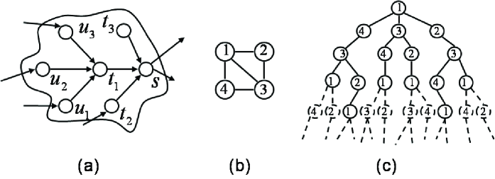
Figure 1: Graphical models: (a) message passing in a portion of a belief network; (b) a simple graph; and (c) Bethe tree (all nodes and edges) and Self-Avoiding Walk tree (black solid only) of (b).

Let us consider a general graphical model $\mathbb{G}=(\mathbb{V},\mathbb{E})$ whose distribution factors as follows:

$$p(X)=\frac{1}{Z}\prod_{(s,t)\in\mathbb{E}}\psi_{st}(x_{s},x_{t})\prod_{s\in\mathbb{V}}\psi_{s}(x_{s}),$$ (1)

where $Z$ is a normalization factor, $\psi_{st}(x_{s},x_{t})$ is the pairwise potential function between random variables $x_{s}$ and $x_{t}$, and $\psi_{s}(x_{s})$ is the single node potential function on $x_{s}$. $(s,t)$ denotes an undirected edge, $\mathbb{V}$ is the set of nodes, and $\mathbb{E}$ is the set of edges. We assume that all the potential functions are positive.

Fig. 1(a) illustrates the message passing mechanism used in BP. The updating rule of the sum-product algorithm for the message sent by node $t$ to its neighbor node $s$ at iteration $i$ is:

$$m_{ts}^{i}(x_{s})\propto\int\psi_{ts}(x_{t},x_{s})\psi_{t}(x_{t})\prod_{u\in\Gamma_{t}\backslash s}m_{ut}^{i-1}(x_{t})dx_{t},$$ (2)

where $\Gamma_{t}$ is the set of neighbors of node $t$. The belief, or pseudo-marginal probability of $x_{t}$, on node $t$ at iteration $i$, is:

$$B_{t}^{i}(x_{t})\propto\psi_{t}(x_{t})\prod_{u\in\Gamma_{t}}m_{ut}^{i}(x_{t}).$$ (3)

A stable fixed point has been reached if $m_{ts}^{i}(x_{s})=m_{ts}^{i+1}(x_{s})$, $\forall s\in\mathbb{V}$. The pairwise belief of random variables $x_{s},x_{t}$ at iteration $i$ is defined as:

$$B_{ts}^{i}(x_{t},x_{s})\propto\psi_{ts}(x_{t},x_{s})\psi_{t}(x_{t})\psi_{s}(x_{s})\prod_{u\in\Gamma_{t}\backslash s}m_{ut}^{i}(x_{t})\prod_{p\in\Gamma_{s}\backslash t}m_{ps}^{i}(x_{s}).$$ (4)

The computation tree first introduced in Wiberg (1996) is always applied in the analysis of LBP. Bethe tree and SAW tree are two types of computation trees used in Ihler (2007), which will also be used in the rest of the paper. Both Bethe tree and SAW tree are tree-structured unwrappings of a graph $\mathbb{G}$ from some node $v$. The Bethe tree, denoted as $T_{B}(\mathbb{G},v,n)$, contains all paths of length $n$ from $v$ that do not backtrack, while the SAW tree, denoted as $T_{SAW}(\mathbb{G},v,n)$, contains all paths of length $n\leq|\mathbb{V}|+1$ that do not backtrack and have all nodes on the path unique. The belief on node $v$ at iteration $n$ in synchronous LBP is equivalent to the exact marginal of the root $v$ in the $n$-level Bethe tree.

Figure 1(c) illustrates the Bethe tree and the SAW tree for the graphical model in Figure 1(b). For synchronous BP, each iteration of Equations (2), (3) and (4) corresponds to a level in the Bethe tree.

2.2 Approaches to Analyze Convergence of LBP

Various approaches have been presented to derive convergence conditions for the sum-product algorithm, including Gibbs measure [Tatikonda and Jordan (2002)], equivalent minimax problem [Heskes (2004)], and contraction property of LBP updates [Ihler et al. (2005); Mooij and Kappen (2007)]. Tatikonda and Jordan (2002) proved that, when the Gibbs measure on the corresponding computation tree is unique, LBP converges to a unique fixed point. Heskes (2004) proved that, when the minima of Bethe free energy is unique, there is a unique fixed point for LBP. Ihler et al. (2005) and Mooij and Kappen (2007) used similar methodology by applying $\ell_{\infty}$ measure on potential functions. They proved that when LBP updating is a contractive mapping, LBP will converge. They both compared their convergence results with those of Tatikonda and Jordan (2002) and Heskes (2004), and showed that their results are stronger. Mooij and Kappen (2007) further showed that they derived more general results than Ihler et al. (2005). Enlightened by the discussion in Ihler et al. (2005) and Mooij and Kappen (2007), and based on the framework of Ihler et al. (2005), we use a new measure on message errors of LBP, in order to obtain distance bound and accuracy bound.

Our contributions are as follows:

1. We present a tight upper- and lower- bound for multiplicative message error $e(x)$ in Section 2.5. Furthermore, based on the upper- and lower- bound, we derive tight uniform distance bound and non-uniform distance bound for beliefs $B(x)$ in Section 3, which help to tighten the accuracy bounds between beliefs and true marginals in Section 5 and correct the upper-bound on message residuals for residual scheduling in Section 6.

2. We investigate the relation between convergence of LBP with sparsity and walk-summability of graphical models in Section 4. We extend walk-summability for Gaussian graphical models to general graphical models and compare the tightness of existing convergence conditions.

3. We analyze the paramagnetic fixed point, ferromagnetic and antiferromagnetic fixed points for uniform binary graphs using message updating functions, and present true message error variation functions to show dynamics of sum-product algorithm in Section 7.

2.3 Message-Error Measures

Define message error as a multiplicative function $e_{ts}^{i}(x_{s})$ that perturbs the fixed-point message $m_{ts}(x_{s})$. The perturbed message at iteration $i$ is hence

$$\hat{m}_{ts}^{i}(x_{s})=m_{ts}(x_{s})e_{ts}^{i}(x_{s}).$$

Dealing with normalized messages, we define fixed-point incoming message products as

$$M_{ts}(x_{t})\propto\psi_{t}(x_{t})\prod_{u\in\Gamma_{t}\backslash s}m_{ut}(x_{t}),$$

and perturbed incoming message products as

$$M_{ts}^{i}(x_{t})\propto\psi_{t}(x_{t})\prod_{u\in\Gamma_{t}\backslash s}m_{ut}^{i}(x_{t}),$$

and incoming error products as

$$E_{ts}^{i}(x_{t})=\prod_{u\in\Gamma_{t}\backslash s}e_{ut}^{i}(x_{t}).$$

We have

$$M_{ts}^{i}(x_{t})\propto M_{ts}(x_{t})E_{ts}^{i}(x_{t}).$$

Thus, the outgoing message error from node $t$ to node $s$ at iteration $i+1$ is:

$$e_{ts}^{i+1}(x_{s})=\frac{\hat{m}_{ts}^{i+1}(x_{s})}{m_{ts}(x_{s})}=\frac{\int\psi_{ts}(x_{t},x_{s})M_{ts}(x_{t})E_{ts}^{i}(x_{t})dx_{t}}{\int\psi_{ts}(x_{t},x_{s})M_{ts}(x_{t})E_{ts}^{i}(x_{t})dx_{t}dx_{s}}\times\frac{\int\psi_{ts}(x_{t},x_{s})M_{ts}(x_{t})dx_{t}dx_{s}}{\int\psi_{ts}(x_{t},x_{s})M_{ts}(x_{t})dx_{t}}.$$

In the following, we will introduce two measures on message errors.

2.3.1 Dynamic-Range Measure

The dynamic-range measure of error introduced by Ihler et al. (2005) is defined as:

$$d(e^{i}_{ts})=\max_{a,b}\sqrt{\frac{e^{i}_{ts}(a)}{e^{i}_{ts}(b)}}.$$ (5)

We have $d(e^{i}_{ts})\to 1$ when $e^{i}_{ts}(x)\to 1$. In  Ihler et al. (2005) [Th.8] it was shown that when $d(\psi_{ts})=\max_{a,b,c,d}\sqrt{\frac{\psi_{ts}(a,b)}{\psi_{ts}(c,d)}}$ is finite, the dynamic-range measure satisfies the following contraction:

$$d(e_{ts}^{i+1})\leq\frac{d(\psi_{ts})^{2}d(E_{ts}^{i})+1}{d(\psi_{ts})^{2}+d(E_{ts}^{i})},$$ (6)

in other words, based on the dynamic-range measure, the outgoing message error is bounded by a non-linear function of the potential function and the incoming error product.

2.3.2 Maximum-Error Measure

To study the dynamics of message error propagation, dealing directly with errors is more interesting than dealing with dynamic range. Moreover, we target to tighten distance bounds of LBP results by using a new error measure. We thus introduce the following maximum multiplicative error function as an error measure:

$$\max_{x_{s}}e^{i+1}_{ts}(x_{s})=\max_{x_{s}}\frac{\int\psi_{ts}(x_{t},x_{s})M_{ts}(x_{t})E^{i}_{ts}(x_{t})dx_{t}}{\int\psi_{t\star}(x_{t})M_{ts}(x_{t})E^{i}_{ts}(x_{t})dx_{t}}\times\frac{\int\psi_{t\star}(x_{t})M_{ts}(x_{t})dx_{t}}{\int\psi_{ts}(x_{t},x_{s})M_{ts}(x_{t})dx_{t}},$$ (7)

where $\psi_{t\star}(x_{t})=\int\psi_{ts}(x_{t},x_{s})dx_{s}$. It is immediate that the maximum-error measure approaches one when multiplicative errors vanish. We will show later that this error measure satisfies the following contraction:

$$\max_{x_{s}}e_{ts}^{i+1}(x_{s})\leq\left(\frac{d(\psi_{ts})d(\psi_{t\star})d(E_{ts}^{i})+1}{d(\psi_{ts})d(\psi_{t\star})+d(E_{ts}^{i})}\right)^{2}.$$ (8)

Dynamic-range measure and maximum-error measure are equivalent when the maximum and minimum of an error function are reciprocal. By comparison, maximum-error measure gives an absolute error, while dynamic-range measure gives a relative error which is invariant to scaling. We will show in the following of the paper that maximum-error measure should be used, when we are interested in absolute errors. Furthermore, both defined in dynamic-range measure, $d(\psi_{ts})$ and $d(\psi_{t\star})$ correspond to two types of matrix norms on $\psi_{ts}$. $d(\psi_{t\star})$ in the RHS of Inequality (8) characterizes the effect of normalization factor on $\max_{x_{s}}e^{i+1}_{ts}(x_{s})$. We will discuss the influence of $d(\psi_{t\star})$ on error bounds in Section 2.5.

2.4 Strength of Potential Functions

Heskes (2004), Ihler et al. (2005) and Mooij and Kappen (2007) have defined measures of strength of potential functions respectively, which help to obtain better convergence conditions than those only related with topology of graphical models. In the following, we will show the relationship between beliefs and strength of pairwise potential functions.

2.4.1 Strength of Potential functions in Heskes (2004)

Heskes (2004) defined $\sigma_{t,s}$ as the strength of a pairwise potential function $\psi_{ts}(x_{t},x_{s})$ meeting the following equation:

$$\frac{1}{1-\sigma_{t,s}}=\max_{x_{t},x_{s},\hat{x}_{t},\hat{x}_{s}}\frac{\psi_{ts}(x_{t},x_{s})\psi_{ts}(\hat{x}_{t},\hat{x}_{s})}{\psi_{ts}(x_{t},\hat{x}_{s})\psi_{ts}(\hat{x}_{t},x_{s})}.$$

This strength is related with the correlation of LBP marginals as follows:

$$\frac{B_{ts}(x_{t},\hat{x}_{s})}{B_{t}(x_{t})B_{s}(\hat{x}_{s})}\leq\frac{1}{1-\sigma_{t,s}},$$

which was then utilized to give a better convergence condition than the one only depending on graph topology.

2.4.2 Strength of Potential functions in Ihler et al. (2005)

Ihler et al. (2005) proposed the dynamic-range measure $d(\psi_{ts})$ as the strength of potential functions $\psi_{ts}(x_{t},x_{s})$. Let us restate the definition of the strength of potential functions and its relationship with message errors in Section 2.3.1 as follows:

$$d(\psi_{ts})=\max_{x_{t},x_{s},\hat{x}_{t},\hat{x}_{s}}\sqrt{\frac{\psi_{ts}(x_{t},x_{s})}{\psi_{ts}(\hat{x}_{t},\hat{x}_{s})}},$$

$$d(e_{ts})\leq\frac{d(\psi_{ts})^{2}d(E_{ts})+1}{d(\psi_{ts})^{2}+d(E_{ts})}.$$

By considering single node potentials $\psi_{t}(x_{t})$ and $\psi_{s}(x_{s})$, Ihler et al. (2005) weakened the strength of pairwise potential functions by using the following dynamic range measure:

$$d(\psi_{ts})^{2}=\min_{\psi_{t},\psi_{s}}d(\frac{\psi_{ts}}{\psi_{t}\psi_{s}})^{2}=\sup_{x_{t},x_{s},\hat{x}_{t},\hat{x}_{s}}\sqrt{\frac{\psi_{ts}(x_{t},x_{s})\psi_{ts}(\hat{x}_{t},\hat{x}_{s})}{\psi_{ts}(\hat{x}_{t},x_{s})\psi_{ts}(x_{t},\hat{x}_{s})}}.$$ (9)

We will apply the strength of potential functions in Equation 9 in our following results.

2.4.3 Strength of Potential functions in Mooij and Kappen (2007)

Mooij and Kappen (2007) mentioned a measure of the strength of potential function $\psi_{ts}(x_{t},x_{s})$, which is defined as:

$$N(\psi_{ts})=\max_{x_{t}\neq\hat{x}_{t},x_{s}\neq\hat{x}_{s}}\frac{\sqrt{\frac{\psi_{ts}(x_{t},x_{s})\psi_{ts}(\hat{x}_{t},\hat{x}_{s})}{\psi_{ts}(\hat{x}_{t},x_{s})\psi_{ts}(x_{t},\hat{x}_{s})}}-1}{\sqrt{\frac{\psi_{ts}(x_{t},x_{s})\psi_{ts}(\hat{x}_{t},\hat{x}_{s})}{\psi_{ts}(\hat{x}_{t},x_{s})\psi_{ts}(x_{t},\hat{x}_{s})}}+1}=\frac{1-\sqrt{1-\sigma_{t,s}}}{1+\sqrt{1-\sigma_{t,s}}}.$$ (10)

They defined log dynamic range measure as metric of errors. Let $\lambda_{ts}$ be the log message reparameterization of message $m_{ts}$. That is,

$$\lambda_{ts}(x_{s})=\log m_{ts}(x_{s}).$$

Denote $\Delta\lambda$ as the difference of log messages. Thus, we have

$$\Delta\lambda_{ts}(x_{s})=\log\hat{m}_{ts}(x_{s})-\log m_{ts}(x_{s})=\log e_{ts}(x_{s}).$$

By the quotient norm and Equation (41) in Mooij and Kappen (2007), we have the following metric of error

$$\|\overline{\Delta\lambda_{ts}}\|=\frac{1}{2}\sup_{x_{s},x^{\prime}_{s}}|\Delta\lambda_{ts}(x_{s})-\Delta\lambda_{ts}(x^{\prime}_{s})|=\log d(e_{ts}).$$ (11)

Using the quotient mapping approach of parallel LBP update in Mooij and Kappen (2007), we will find the relationship between the strength of potential functions in Equation (10) and the metric of message errors in Equation (11) in the following.

Because $\|\overline{\Delta\lambda_{ts}}\|\leq\sum_{u\in\Gamma_{t}\backslash s}\|\overline{\frac{\partial\lambda_{ts}}{\partial\lambda_{ut}}}\|\|\overline{\Delta\lambda_{ut}}\|$ and $\|\overline{\frac{\partial\lambda_{ts}}{\partial\lambda_{ut}}}\|\leq N(\psi_{ts})$ by Equation (36-45) in Mooij and Kappen (2007), we have

$$\log d(e_{ts})\leq N(\psi_{ts})\sum_{u\in\Gamma_{t}\backslash s}\log d(e_{ut})\leq N(\psi_{ts})\log d(E_{ts}),$$

$$or,\quad d(e_{ts})\leq d(E_{ts})^{N(\psi_{ts})}.$$

We can observe that the smaller $N(\psi_{ts})$ is, the smaller is $d(e_{ts})$; therefore, the faster is the contraction of errors. The previous inequality reveals another result on contractive property of message errors beside the one in Equation (6).

In the following, we use the maximum-error measure in Equation (7) to explore upper and lower bounds on message errors, and upper bounds on the distances between beliefs.

2.5 Upper- and Lower-Bounds on Message Errors

We have the multiplicative error function as follows:

$$e^{i+1}_{ts}(x_{s})=\frac{\int\psi_{ts}(x_{t},x_{s})M_{ts}(x_{t})E^{i}_{ts}(x_{t})dx_{t}}{\int\psi_{t\star}(x_{t})M_{ts}(x_{t})E^{i}_{ts}(x_{t})dx_{t}}\times\frac{\int\psi_{t\star}(x_{t})M_{ts}(x_{t})dx_{t}}{\int\psi_{ts}(x_{t},x_{s})M_{ts}(x_{t})dx_{t}},$$

where $\psi_{t\star}(x_{t})=\int\psi_{ts}(x_{t},x_{s})dx_{s}$. We will show that the error function is upper- and lower- bounded.

Theorem 1

Multiplicative outgoing errors are bounded as:

$$\left(\frac{d(\psi_{ts})d(\psi_{t\star})+d(E_{ts})}{d(\psi_{ts})d(\psi_{t\star})d(E_{ts})+1}\right)^{2}\leq\min_{x_{s}}e_{ts}(x_{s})\leq e_{ts}(x_{s})\leq\max_{x_{s}}e_{ts}(x_{s})\leq\left(\frac{d(\psi_{ts})d(\psi_{t\star})d(E_{ts})+1}{d(\psi_{ts})d(\psi_{t\star})+d(E_{ts})}\right)^{2}.$$

The proof appears in Appendix A.

Let us use the following denotation for our upper-bound:

$$\Delta_{1}=\left(\frac{d(\psi_{ts})d(\psi_{t\star})d(E_{ts})+1}{d(\psi_{ts})d(\psi_{t\star})+d(E_{ts})}\right)^{2}.$$ (12)

From (Ihler et al., 2005, Th.2 and Th.8), we can derive their upper-bound for $\max_{x_{s}}e_{ts}(x_{s})$:

$$\max_{x_{s}}e_{ts}(x_{s})\leq d(e_{ts})^{2}\leq\left(\frac{d(\psi_{ts})^{2}d(E_{ts})+1}{d(\psi_{ts})^{2}+d(E_{ts})}\right)^{2}=\Delta_{2}.$$ (13)

Theorem 2

The upper bound $\Delta_{1}$ on the multiplicative error provided in Theorem 1 is tighter than the upper bound $\Delta_{2}$ from (Ihler et al., 2005, Th.2 and Th.8):

Proof  Because $\Delta_{1}$ in (12) is increasing in $d(\psi_{t\star})$ we conclude that (12) implies (13), i.e., $\Delta_{1}\leq\Delta_{2}$, because

$$d(\psi_{t\star})=\max_{a,b}\sqrt{\frac{\psi_{t\star}(a)}{\psi_{t\star}(b)}}=\max_{a,b}\sqrt{\frac{\int\psi_{ts}(a,x_{s})dx_{s}}{\int\psi_{ts}(b,x_{s})dx_{s}}}$$

$$\leq\max_{a,b}\sqrt{\max_{c,d}\frac{\psi_{ts}(a,c)}{\psi_{ts}(b,d)}}=\max_{a,b,c,d}\sqrt{\frac{\psi_{ts}(a,c)}{\psi_{ts}(b,d)}}=d(\psi_{ts}).$$

 

We can see how $d(\psi_{t\star})$ tightens the upper-bound by analyzing the log-distance between $\Delta_{1}$ and $\Delta_{2}$. Let $d(\psi_{t\star})=Kd(\psi_{ts})$, where $1/d(\psi_{ts})\leq K\leq 1$. Therefore, the log-distance between $\Delta_{1}$ and $\Delta_{2}$ is denoted as

$$D(K)=\log{\Delta_{1}}-\log{\Delta_{2}}=2\times\log{\{\frac{Kd(\psi_{ts})^{2}d(E_{ts})+1}{Kd(\psi_{ts})^{2}+d(E_{ts})}\times\frac{d(\psi_{ts})^{2}+d(E_{ts})}{d(\psi_{ts})^{2}d(E_{ts})+1}\}}.$$

We can easily find that the first gradient $D^{(1)}(K)>0$ when $d(E_{ts})>1$. Thus, the maximum log-distance between $\Delta_{1}$ and $\Delta_{2}$ is obtained at $K=1/d(\psi_{ts})$. In other words, when $d(\psi_{t\star})=1$, our upper-bound $\Delta_{1}$ is tighter than $\Delta_{2}$ at farthest.

3 Distance Bounds on Beliefs

In the study of convergence, we are interested to know how beliefs will vary at each iteration, when LBP fails to converge. We will show that beliefs are bounded given the strength of potential functions and the structure of the graph. In the following, we will present our uniform distance bound and non-uniform distance bound on beliefs. Based on those bounds, we further present uniform convergence condition and non-uniform convergence condition for synchronous LBP.

3.1 Uniform Distance Bound

Corollary 3

(Uniform Distance Bound)
The log-distance bound of fixed points on belief at node $s$ is

$$\sum_{t\in\Gamma_{s}}\log(\frac{d(\psi_{ts})d(\psi_{t\star})\varepsilon+1}{d(\psi_{ts})d(\psi_{t\star})+\varepsilon})^{2},$$

where $\varepsilon$ should satisfy

$$\log{\varepsilon}=\max_{(s,p)\in\mathbb{E}}\sum_{t\in\Gamma_{s}\backslash p}\log({\frac{d(\psi_{ts})d(\psi_{t\star})\varepsilon+1}{d(\psi_{ts})d(\psi_{t\star})+\varepsilon}})^{2}.$$

The proof appears in Appendix A.

Let us reintroduce the error bound-variation function used in the proof for Corollary 3:

$$G_{sp}^{O}(\log{\varepsilon})=\log{\prod_{t\in\Gamma_{s}\backslash p}(\frac{d(\psi_{ts})d(\psi_{t\star})\varepsilon+1}{d(\psi_{ts})d(\psi_{t\star})+\varepsilon}})^{2}-\log{\varepsilon},\varepsilon\geq 1.$$ (14)

Adopting the upper-bound $\Delta_{2}$ in (13), the error bound-variation function is:

$$G_{sp}^{I}(\log{\varepsilon})=\log{\prod_{t\in\Gamma_{s}\backslash p}(\frac{d(\psi_{ts})^{2}\varepsilon+1}{d(\psi_{ts})^{2}+\varepsilon}})^{2}-\log{\varepsilon},\varepsilon\geq 1.$$ (15)

Those error bound-variation functions describe the upper-bound on variation of maximal message errors throughout the belief networks. We can see that $G_{sp}^{O}(\log{\varepsilon})<G_{sp}^{I}(\log{\varepsilon})$. In other words, the error bound-variation function using our upper-bound $\Delta_{1}$ is tighter than that using Ihler et al. (2005)’s upper-bound $\Delta_{2}$, which is illustrated in Fig. 2. However, in Ihler et al. (2005), they used the following error bound-variation function:

$$G_{sp}^{II}(\log{\varepsilon^{\prime}})=\log{\prod_{t\in\Gamma_{s}\backslash p}(\frac{d(\psi_{ts})^{2}\varepsilon^{\prime}+1}{d(\psi_{ts})^{2}+\varepsilon^{\prime}}})-\log{\varepsilon^{\prime}},$$ (16)

where $\varepsilon^{\prime}$ is an upper-bound on dynamic range measure $d(E_{ts})$. Since our $\varepsilon$ is an upper-bound on maximum error measure $\max{E_{ts}}$, it’s hard to compare $G_{sp}^{O}(\log{\varepsilon})$ and $G_{sp}^{II}(\log{\varepsilon^{\prime}})$. In other words, we cannot say our Uniform Distance Bound in Corollary 3 is better than that in (Ihler et al., 2005, Theorem 13).

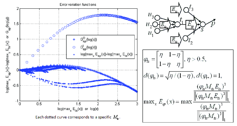
Figure 2: Error bound-variation functions versus true error-variation function for the local graph of node s. Potential functions on edges $(t_{1},s),(t_{2},s),(t_{3},s)$ are the same, where $\eta=0.7$. We also impose the same incoming error product $E_{ts}$ on nodes $t_{1},t_{2},t_{3}$. The dotted curves depict the true error variation functions, $\{\log{\max_{x}E_{sp}(x)}-\log{\max_{x}E_{ts}(x)},t\in\Gamma_{s}\backslash p\}$, which are enveloped by our error bound-variation function $G_{sp}^{O}(\log{\varepsilon})$.

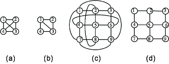
Figure 3: Four simple graphical models: (a) a four-node fully connected graph; (b) a partial graph that has one less edge than (a); (c) a nine-node graph with uniform degree; and (d) a $3\times 3$ grid that is a partial graph of (c).

When the error bound-variation function is always less than zero, the maximum of error bounds decreases after each iteration of LBP. In other words, LBP will converge. Therefore, our uniform distance bound in Corollary 3 will lead to a sufficient condition for convergence of LBP.

Theorem 4

(Uniform Convergence Condition)
Based on maximum-error measure, the sufficient condition for the sum-product algorithm to converge to a unique fixed point is

$$\max_{(s,p)\in\mathbb{E}}\sum_{t\in\Gamma_{s}\backslash p}\frac{d(\psi_{ts})d(\psi_{t\star})-1}{d(\psi_{ts})d(\psi_{t\star})+1}<\frac{1}{2}.$$

The proof appears in Appendix A.

Since we cannot compare $G_{sp}^{O}(\log{\varepsilon})$ and $G_{sp}^{II}(\log{\varepsilon^{\prime}})$ directly because $\varepsilon$ and $\varepsilon^{\prime}$ correspond to different measures, let us take the maximum of the two measures and deal with it as a new measure. Specifically, let $\tilde{\varepsilon}=\max\{\varepsilon,\varepsilon^{\prime}\}$. After some calculation, we can find that $G_{sp}^{O}(\log{\tilde{\varepsilon}})$ is greater than $G_{sp}^{II}(\log{\tilde{\varepsilon}})$. In other words, $G_{sp}^{II}(\log{\tilde{\varepsilon}})$ is tighter than $G_{sp}^{O}(\log{\tilde{\varepsilon}})$. Therefore, the convergence condition derived from $G_{sp}^{II}(\log{\tilde{\varepsilon}})$ will be better. The following lemma provides a proof for this observation.

Lemma 5

Our sufficient condition $\sum_{t\in\Gamma_{s}\backslash p}\frac{d(\psi_{ts})d(\psi_{t\star})-1}{d(\psi_{ts})d(\psi_{t\star})+1}<\frac{1}{2}$ is worse than the sufficient condition in Ihler et al. (2005), which is $\sum_{t\in\Gamma_{s}\backslash p}\frac{d(\psi_{ts})^{2}-1}{d(\psi_{ts})^{2}+1}<1$.

Proof  $2(\frac{d(\psi_{ts})d(\psi_{t\star})-1}{d(\psi_{ts})d(\psi_{t\star})+1})>\frac{d(\psi_{ts})^{2}-1}{d(\psi_{ts})^{2}+1}$.  

Our failure to improve the uniform convergence condition by using maximum-error measure shows that dynamic-range measure is better than maximum-error measure with respect to the sensitivity of the measure to convergence. Nevertheless, as for the upper bound on a multiplicative message error $e_{ts}(x)$, maximum-error measure gives a tighter result, which is shown in Theorem 2. Furthermore, the maximum-error measure may provide better distance bounds for beliefs.

Inspired by the sensitivity of dynamic-range measure to convergence, we present the following improved uniform distance bound, which first calculates the fixed-point values of error bounds in dynamic-range measure, and then computes the error bounds among beliefs in maximum-error measure.

Corollary 6

(Improved Uniform Distance Bound)
The log-distance bound of fixed points on belief at node $s$ is

$$\sum_{t\in\Gamma_{s}}\log(\frac{d(\psi_{ts})d(\psi_{t\star})\varepsilon+1}{d(\psi_{ts})d(\psi_{t\star})+\varepsilon})^{2},$$

where $\varepsilon$ should satisfy

$$\log{\varepsilon}=\max_{(s,p)\in\mathbb{E}}\sum_{t\in\Gamma_{s}\backslash p}\log{\frac{d(\psi_{ts})^{2}\varepsilon+1}{d(\psi_{ts})^{2}+\varepsilon}}.$$

Proof  Using the approach in (Ihler et al., 2005, Theorem 12) to obtain distance bounds on incoming error products in dynamic-range measure and applying our Theorem 1, we obtain our corollary.  

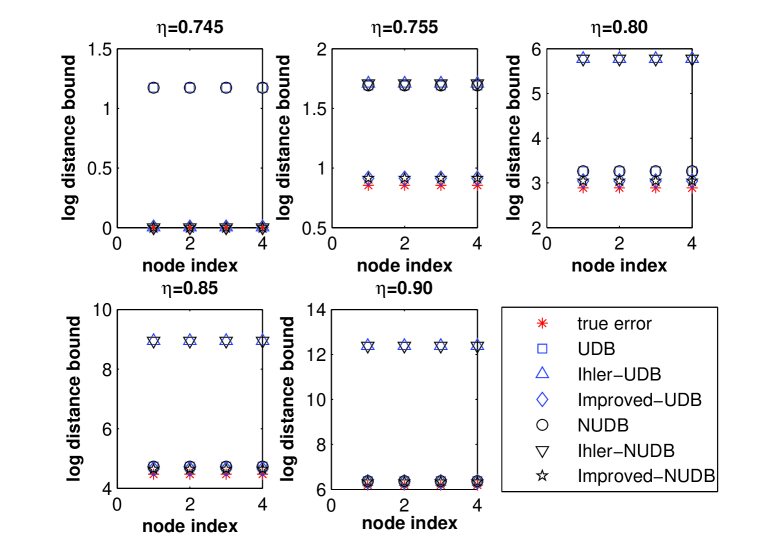
Figure 4: True distance, uniform distance bounds and non-uniform distance bounds for the graph in  3(a) with various $\eta$’s. The empirical critical value of $\eta$ for LBP to converge is $\eta<0.75$.

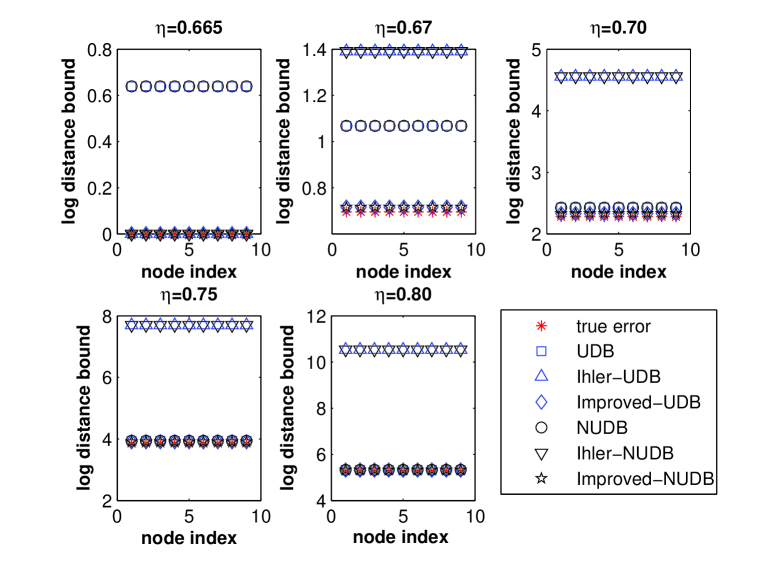
Figure 5: True distance, uniform distance bounds and non-uniform distance bounds for the graph in  3(c) with various $\eta$’s. The empirical critical value of $\eta$ for LBP to converge is $\eta<0.67$.

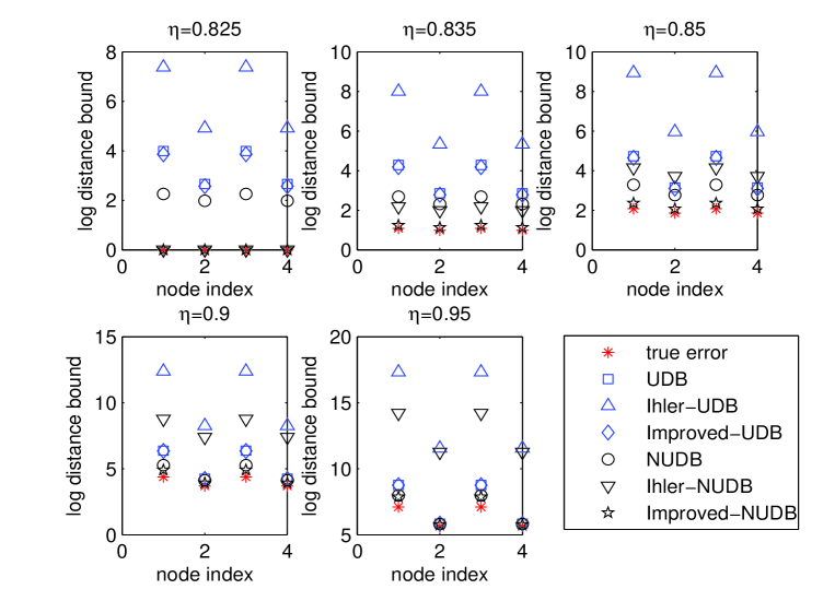
Figure 6: True distance, uniform distance bounds and non-uniform distance bounds for the graph in  3(b) with various $\eta$’s. The empirical critical value of $\eta$ for LBP to converge is $\eta<0.83$.

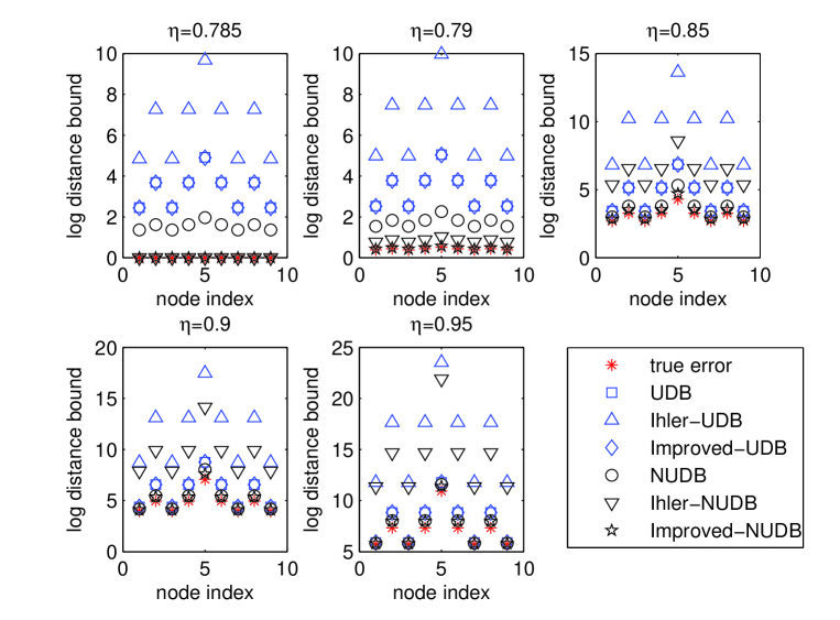
Figure 7: True distance, uniform distance bounds and non-uniform distance bounds for the graph in  3(d) with various $\eta$’s. The empirical critical value of $\eta$ for LBP to converge is $\eta<0.79$.

Let see how our uniform distance bound and improved uniform distance bound perform for graphical models in Fig. 3 by comparison to the Fixed-point distance bound in Ihler et al. (2005). Let all the pairwise potential functions be $\begin{pmatrix}\eta&1-\eta\\ 1-\eta&\eta\end{pmatrix}$ where $\eta>0.5$ and all the single node potentials be $\begin{pmatrix}1\\ 1\end{pmatrix}$. Therefore, $d(\psi_{ts})=\sqrt{\eta/(1-\eta)}$ and $d(\psi_{t\star})=1$ for $\forall~{}(t,s)\in\mathbb{E}$.

We compare the following bounds in our simulations: UDB, our uniform distance bound in Corollary 3; Improved-UDB, our improved uniform distance bound in Corollary 6; Ihler-UDB, Fixed-point distance bound in (Ihler et al., 2005, Theorem 13). Fig.4 - Fig. 7 illustrate the performances of those bounds for graphs in Figs. 3(a), (c), (b) and (d), respectively.

Graphs in Figs. 3(a) and (c) are uniform (uniform degrees, uniform potential functions). Given a specific $\eta$, all nodes have the same distance bound. The critical value of $\eta$ is the value beyond which LBP will not converge. For those two graphs, the empirical critical values of $\eta$ with respect to the convergence of LBP are $0.75$ and $0.67$ respectively. We can see that, for various $\eta$’s, our Improved-UDBs are very close to the true errors between beliefs. Our UDBs become tighter when $\eta$ increases, while Ihler-UDBs become looser. From Fig. 4 and Fig. 5, we can see that, compared to Ihler-UDB, our UDB requires stricter critical values of $\eta$ to ensure error bounds to be zeros. Specifically, for Fig. 4, when $\eta=0.745$, our UDBs are non-zeros and Ihler-UDBs are zeros; hence, our UDB requires $\eta<0.745$ for the convergence of LBP, while Ihler-UDB only requires $\eta<0.75$. Nevertheless, the critical values by our UDB are $0.735$ for Fig. 3(a) and $0.66$ for Fig. 3(c), which are close to the empirical critical values. Based on our UDB and Ihler-UDB, our Improved-UDBs will approximate zeros when $\eta$ approaches $0.75$ and give tightest distance bounds for any $\eta$.

3.2 Non-Uniform Distance Bound

Fig. 3(b) and Fig. 3 (d) are non-uniform graphs. Because uniform distance bounds are computed locally, beliefs on the nodes with different topologies will have different error bounds, which can be observed from Fig. 6 and Fig. 7. We can also find that when the true errors are zeros, uniform bounds are not all zeros. In other words, $\eta$ must be smaller than the empirical critical value to ensure the largest uniform distance bounds to be zero. Furthermore, in such cases, uniform convergence conditions derived from uniform distance bounds will not perform well as for uniform graphs. Therefore, when every loop contains potentials with various strengths and each node has different topology, we present the following non-uniform distance bound and improved non-uniform distance bound.

Corollary 7

(Non-uniform Distance Bound)
The non-uniform log-distance bound of fixed points on belief at node $s$ after $n\geq 1$ iterations is

$$\sum_{t\in\Gamma_{s}}\log(\frac{d(\psi_{ts})d(\psi_{t\star})\varepsilon^{n}_{ts}+1}{d(\psi_{ts})d(\psi_{t\star})+\varepsilon^{n}_{ts}})^{2},$$

where $\varepsilon^{i}_{ts}$ is updated by

$$\log{\varepsilon^{i}_{ts}}=\sum_{u\in\Gamma_{t}\backslash s}\log({\frac{d(\psi_{ut})d(\psi_{u\star})\varepsilon^{i-1}_{ut}+1}{d(\psi_{ut})d(\psi_{u\star})+\varepsilon^{i-1}_{ut}}})^{2}$$

with initial condition

$$\log\varepsilon^{1}_{ut}=\sum_{v\in\Gamma_{u}\backslash t}\log(d(\psi_{vu})d(\psi_{v\star}))^{2}.$$

Proof  The result can be easily proved from Corollary 3, by defining the error bound-variation function in (14) as follows:

$$G_{ts}(\log{\varepsilon_{ts}^{i}})=\log\prod_{u\in\Gamma_{t}\backslash s}\Delta_{ut}(\varepsilon_{ut}^{i-1})-\log{\varepsilon_{ts}^{i}}=\sum_{u\in\Gamma_{t}\backslash s}\log({\frac{d(\psi_{ut})d(\psi_{u\star})\varepsilon^{i-1}_{ut}+1}{d(\psi_{ut})d(\psi_{u\star})+\varepsilon^{i-1}_{ut}}})^{2}-\log{\varepsilon^{i}_{ts}}.$$

 
Similarly, based on the fact that the dynamic-range measure gives better convergence condition than the maximum-error measure, we improve the previous non-uniform distance bound in the following.

Corollary 8

(Improved Non-uniform Distance Bound)
The improved non-uniform log-distance bound of fixed points on belief at node $s$ after $n\geq 1$ iterations is

$$\sum_{t\in\Gamma_{s}}\log(\frac{d(\psi_{ts})d(\psi_{t\star})\varepsilon^{n}_{ts}+1}{d(\psi_{ts})d(\psi_{t\star})+\varepsilon^{n}_{ts}})^{2},$$

where $\varepsilon^{i}_{ts}$ is updated by

$$\log{\varepsilon^{i}_{ts}}=\sum_{u\in\Gamma_{t}\backslash s}\log{\frac{d(\psi_{ut})^{2}\varepsilon^{i-1}_{ut}+1}{d(\psi_{ut})^{2}+\varepsilon^{i-1}_{ut}}}$$

with initial condition $\log\varepsilon^{1}_{ut}=\sum_{v\in\Gamma_{u}\backslash t}\log d(\psi_{vu})^{2}$.

Proof  Using the approach in (Ihler et al., 2005, Theorem 14) to obtain distance bounds on incoming error products in dynamic-range measure and applying our Theorem 1, we obtain our corollary.  

Let see the performaces of our non-uniform distance bound and improved non-uniform distance bound for the graphs in Fig. 3 compared with the non-uniform distance bound in (Ihler et al., 2005, Thm. 14). We denote the bounds in our simulation as follows: NUDB, our non-uniform distance bound in Corollary 7; Improved-NUDB, our improved non-uniform distance bound in Corollary 8; Ihler-NUDB, non-uniform distance bound in (Ihler et al., 2005, Theorem 14).

For uniform graphs in Fig. 3(a) and (c), NUDB performs exactly the same as UDB. However, for non-uniform graphs in Fig. 3(b) and (d), because NUDB propagates error bounds throughout the whole graph rather than on a local neighborhood, NUDBs are tighter than UDBs, which can be observed from Fig. 6 and Fig. 7. For various $\eta$’s, our Improved-NUDBs always approach the true errors. Therefore, when our Improved-NUDB is zero, $\eta$ almost equals the empirical critical value to ensure convergence of LBP. Though worse than Improved-NUDB, our NUDB performs better than Ihler-NUDB when $\eta$ is far way from the area of convergence.

3.2.1 Non-Uniform Convergence

Based on our Improved-NUDB or Ihler-NUDB, a sufficient convergence condition of LBP can be derived, which is based on the dynamic-range measure of propagating errors.

For each cycle-involved vertex $v$, $T(\mathbb{G},v)$ is the corresponding computation tree. Let $\mathbb{V}$ be the set of vertices in the computation tree. For $w_{i}\in\mathbb{V},i=0,...,|\mathbb{V}|-1$, $l(w_{i})$ is the labelling function which maps $w_{i}$ to the original vertex in $\mathbb{G}$. Let $l(w_{0})=v$.

Theorem 9

(Non-Uniform Convergence Condition)
For a graphical model $\mathbb{G}(\mathbb{V},\mathbb{E})$, $\{T(\mathbb{G},v),v\in\mathbb{V}\}$ is the set of computation trees. Let $\mathbb{\bar{E}}$ denote the set of directed edges. For each $T(\mathbb{G},v),v\in\mathbb{V}$, given $vu\in\mathbb{\bar{E}}$, $\mathcal{H}_{vu}$ denotes an expression on edge $vu$:

$$\mathcal{H}_{vu}=\sum_{w_{i}\in\Gamma_{v}\backslash u}\frac{d(\psi_{l(w_{i})v})^{2}-1}{d(\psi_{l(w_{i})v})^{2}+1}\sum_{w_{j}\in\Gamma_{w_{i}}\backslash v}\frac{d(\psi_{l(w_{j})l(w_{i})})^{2}-1}{d(\psi_{l(w_{j})l(w_{i})})^{2}+1}...\sum_{w_{r}\in\Gamma_{w_{q}}\backslash w_{p}}\frac{d(\psi_{l(w_{r})l(w_{q})})^{2}-1}{d(\psi_{l(w_{r})l(w_{q})})^{2}+1},$$ (17)

where $\Gamma_{w_{i}}$ is the set of neighbors of $w_{i}$. The non-uniform sufficient condition for the sum-product algorithm to converge to a local stable fixed point is:

$$\max_{vu\in\mathbb{\bar{E}}}\mathcal{H}_{vu}<1.$$

The proof appears in Appendix A. Based on the type of computation tree, the non-uniform convergence condition will be called non-uniform convergence condition based on $N$-th level Bethe tree, or non-uniform convergence condition based on infinite Bethe tree, or non-uniform convergence condition based on SAW tree. Our non-uniform convergence condition based on infinite Bethe tree is equivalent to (Ihler et al., 2005, Theorem 14).

When a graph has uniform potential functions with strength $d(\psi)$, to ensure convergence, it is sufficient to have

$$\max_{vu\in\mathbb{\bar{E}}}\sum_{w_{i}\in\Gamma_{v}\backslash u}\frac{d(\psi)^{2}-1}{d(\psi)^{2}+1}\sum_{w_{j}\in\Gamma_{w_{i}}\backslash v}\frac{d(\psi)^{2}-1}{d(\psi)^{2}+1}...\sum_{w_{r}\in\Gamma_{w_{q}}\backslash w_{p}}\frac{d(\psi)^{2}-1}{d(\psi)^{2}+1}<1.$$ (18)

Let us apply our non-uniform convergence condition based on SAW tree to the graphs in Fig. 3(b) and (d) with uniform potential functions as in the previous simulations. For the graph in Fig. 3(b), we obtain the critical value $\eta<0.78$ for convergence of LBP, which is closer to the empirical value $\eta<0.83$, compared to $\eta<0.75$ obtained by uniform convergence condition. For the graph in Fig. 3(d), we obtain the critical value $\eta<0.77$, while the empirical value is $\eta<0.79$ and the critical value obtained by uniform convergence condition is $\eta<0.67$. Therefore, our non-uniform convergence condition is tighter than our uniform convergence condition. However, since our non-uniform convergence condition is derived from (Ihler et al., 2005, Theorem 14), we do not improve the convergence condition. Rather than in the form of distance bound in (Ihler et al., 2005, Theorem 14), we express the convergence condition explicitly, which will be used in our later analysis of walk-summability of graphical models. Furthermore, we improve distance bounds between beliefs in Corollary 6 and Corollary 8, which are useful in tightening accuracy bounds in Section 5.

4 Convergence of Loopy Belief Propagation

4.1 Sparsity and Convergence

It lacks theoretical verification that the more sparse a graph is, the less stricter is its convergence condition. Since the definition of sparse graphs is vague, to be confined, we would relate sparsity with partial graphs. In this section, we will show that when LBP converges on one graph in a partial graph set, convergence properties of other graphs can be deduced through our Theorem 9. Let us define partial graphs and introduce the convergence property of such graphs in the following.

Definition 10

(Walk)
In a graph G(V,E), a walk of length $l$ is a sequence of nodes $w=(v_{0},v_{1},...,v_{l})$, $v_{i}\in V$, such that each step of walk $(v_{i},v_{i}+1)$ corresponds to an edge in $E$.

Definition 11

(Prime Cycle)
A closed walk is called a prime cycle if it is not backtracking and not a repeated concatenation of a shorter closed walk.

Definition 12

(Reduction)
A walk composed of two edges $(v_{1},v_{2})$ and $(v_{2},v_{3})$ can be reduced to a walk composed of one edge $(v_{1},v_{3})$, where $\psi_{v_{1}v_{3}}(x_{v_{1}},x_{v_{3}})=\int_{x_{v_{2}}}\psi_{v_{1}v_{2}}(x_{v_{1}},x_{v_{2}})\psi_{v_{2}v_{3}}(x_{v_{2}},x_{v_{3}})dx_{v_{2}}$, when there is no branch on the walk.

Definition 13

(Extension)
A walk composed of one edge $(v_{1},v_{3})$ can be extended to a walk composed of two edges $(v_{1},v_{2})$ and $(v_{2},v_{3})$, where $\int_{x_{v_{2}}}\psi_{v_{1}v_{2}}(x_{v_{1}},x_{v_{2}})\psi_{v_{2}v_{3}}(x_{v_{2}},x_{v_{3}})dx_{v_{2}}=\psi_{v_{1}v_{3}}(x_{v_{1}},x_{v_{3}})$.

It is not hard to prove that Reduction and Extension do not change the convergence property of the original graph. Comparatively, Ruozzi and Tatikonda (2010) splitted some edges and reparameterized the original graphical model in order to obtain a convergent and correct message passing algorithm.

Definition 14

(Partial Graphs)
For two graphical models $\mathbb{G}_{1}(\mathbb{V}_{1},\mathbb{E}_{1})$ and $\mathbb{G}_{2}(\mathbb{V}_{2},\mathbb{E}_{2})$ after reduction and extension, there exists an isomorphism between graphs $\mathbb{G}_{1}(\mathbb{V}_{1},\mathbb{E}_{1})$ and $\mathbb{G}_{2}(\mathbb{V}_{2}^{\ast},\mathbb{E}_{2}^{\ast})$, when $\mathbb{V}_{2}^{\ast}\subseteq\mathbb{V}_{2}$ and $\mathbb{E}_{2}^{\ast}\subset\mathbb{E}_{2}$. When $\mathbb{E}_{2}-\mathbb{E}_{2}^{\ast}$ is cycle-involved, we call $\mathbb{G}_{1}$ a partial graph of $\mathbb{G}_{2}$ and denote it as $\mathbb{G}_{1}\subset\mathbb{G}_{2}$.

Theorem 15

(Strictness of Convergence Condition for Two Partial Graphs)
Given $\mathbb{G}_{1}$ and $\mathbb{G}_{2}$ as defined in Definition 14, assume that $\mathbb{G}_{1}\subset\mathbb{G}_{2}$. Assume the dynamic-range measures of potential functions for edges in $\mathbb{E}_{1}$ are not greater than those of potential functions for corresponding edges in $\mathbb{E}_{2}^{\ast}$. Then, when LBP for $\mathbb{G}_{2}(\mathbb{V}_{2},\mathbb{E}_{2})$ converges, LBP for $\mathbb{G}_{1}(\mathbb{V}_{1},\mathbb{E}_{1})$ must converge; however, the reverse implication is not true in general.

Proof  Because $\mathbb{G}_{1}\subset\mathbb{G}_{2}$ and $\mathbb{E}_{2}-\mathbb{E}_{2}^{\ast}$ are cycle-involved, $T_{B}(\mathbb{G}_{1},v,n)\subset T_{B}(\mathbb{G}_{2},v,n)$. Therefore, the expression in (17) for $\mathbb{G}_{2}$ has more summands than that for $\mathbb{G}_{1}$. When $\mathbb{G}_{2}$ satisfies the convergence condition in Theorem 9, $\mathbb{G}_{1}$ must satisfy it. However, when $\mathbb{G}_{1}$ satisfies the convergence condition, $\mathbb{G}_{2}$ may not satisfy it.  
When the potential functions of a graph are uniform, we have the following corollary.

Corollary 16

(Critical Values of Convergence for Two Partial Graphs)
Given $\mathbb{G}_{1}\subset\mathbb{G}_{2}$, $\mathbb{G}_{1}$ and $\mathbb{G}_{2}$ have uniform potential functions $\psi_{i}=\begin{pmatrix}\eta_{i}&1-\eta_{i}\\ 1-\eta_{i}&\eta_{i}\end{pmatrix},i=1,2$ on all edges. Then, the critical values for convergence of LBP satisfy $\eta_{2}<\eta_{1}$.

Proof  Because (18) for $\mathbb{G}_{2}$ has more summands than that for $\mathbb{G}_{1}$, we easily have $d(\psi_{2})<d(\psi_{1})$ to satisfy the inequality. Because $d(\psi_{i})=\sqrt{\eta_{i}/(1-\eta_{i})}$, we get $\eta_{2}<\eta_{1}$.  
Our Theorem 15 and Corollary 16 can be easily extended to strictness of convergence condition of LBP for a set of partial graphs, and for those with uniform potential functions.

Corollary 17

(Strictness of Convergence Condition for Set of Partial Graphs)
Given $\mathbb{G}_{1}\subset\mathbb{G}_{2}...\subset\mathbb{G}_{N}$, assuming the dynamic-range measures of potential functions on isomorphous edges of those graphs are correspondingly non-decreasing in the previous partial order, LBP convergence for $\mathbb{G}_{j}$ implies LBP convergence for $\mathbb{G}_{i}$, where $i<j$ and $i,j=1,...,N$. However, the reverse implication is not true in general.

Proof  For any $\mathbb{G}_{i}\subset\mathbb{G}_{j}$ in the set of $\{\mathbb{G}_{i},1\leq i\leq N\}$, according to Theorem 15, we have the convergence of $\mathbb{G}_{j}$ implies the convergence of $\mathbb{G}_{i}$.  

Corollary 18

(Critical Value of Convergence for Set of Partial Graphs)
Given $\mathbb{G}_{1}\subset\mathbb{G}_{2}...\subset\mathbb{G}_{k}$, $\mathbb{G}_{1}$,…, $\mathbb{G}_{k}$ have uniform potential functions $\begin{pmatrix}\eta_{i}&1-\eta_{i}\\ 1-\eta_{i}&\eta_{i}\end{pmatrix},1\leq i\leq k$ on all edges. Then, the critical values for convergence of LBP satisfy $\eta_{k}<\eta_{k-1}...<\eta_{1}$.

Proof  For any $\mathbb{G}_{i}\subset\mathbb{G}_{j}$ in the set of $\{\mathbb{G}_{i},1\leq i\leq N\}$, according to Corollary 16, we have the convergence of $\eta_{j}<\eta_{i}$.  

By our Corollary 17 on partially ordered graphs, we can conclude that graphs with less cycle-induced edges are more sparse and thus have weaker convergence condition. It is intuitively true that the strength of potential functions for Fig. 3(a) or Fig. 3(c) should be weaker than that for Fig. 3(b) or Fig. 3(d) to ensure convergence of LBP. This observation can be soundly verified by our previous corollaries.

4.2 Walk-Summability and Convergence

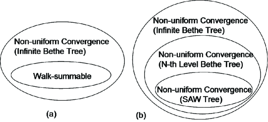
Figure 8: Diagram summarizing mildness of convergence conditions. The SAW tree is a partial tree of the $N$-level Bethe tree, therefore, convergence condition based on the SAW tree is stronger.

Malioutov et al. (2006) related the convergence of LBP with the spectral radius of partial correlation matrix of Gaussian graphical model, for which they introduced a concept called walk-summability. We observe similarity between walk-summability of Gaussian graphical model and our convergence condition for general graphcial model discussed in Section 3.2.1. Therefore, based on some existing works in literature, we extend the walk-summability defined in Malioutov et al. (2006) to that for general graphical models.

A Gaussian graphical model is defined by an undirected graph $G(V,E)$, where $V$ is the set of nodes and $E$ is the set of edges, and a set of jointly Gaussian random variables $\{x_{i},i\in V\}$. The joint density function is defined as follows:

$$p(X)\propto\exp\{-\frac{1}{2}\textsc{x}^{T}J\textsc{x}+h^{T}\textsc{x}\},$$

where $J$ is a symmetric and positive definite matrix called information matrix and $h$ is a potential vector. The partial correlation coefficient between random variable $x_{i}$ and $x_{j}$ is defined as follows:

$$r_{ij}\triangleq\frac{\textrm{cov}(x_{i},x_{j}|x_{V\backslash ij})}{\sqrt{\textrm{var}(x_{i}|x_{V\backslash ij})\textrm{var}(x_{j}|x_{V\backslash ij})}}=-\frac{J_{ij}}{\sqrt{J_{ii}J_{jj}}}.$$

A walk is defined in Definition 10. The weight $\phi(w)$ of a walk $w=(v_{0},v_{1},...,v_{l(w)})$ with length $l(w)$ is defined as:

$$\phi(w)=\prod_{k=1}^{l(w)}r_{v_{k-1}v_{k}}.$$ (19)

Definition 19

(Malioutov et al. (2006))(Walk-Summable)
A Gaussian distribution is walk-summable if for all $i,j\in V$ the unordered walk $w$ from $i$ to $j$, $\sum_{w:i\rightarrow j}\phi(w)$, is well defined.

Proposition 20

(Malioutov et al. (2006))(Walk-Summability)
Let $R$ be a partial correlation coefficient matrix of a Gaussian graphical model, of which diagonal entries are zeros. Each of the following conditions are equivalent to walk-summability:
(i) $\sum_{w:i\rightarrow j}|\phi(w)|$ converges for all $i,j\in V$,
(ii) $\sum_{l}\bar{R}^{l}$ converges, where $\bar{R}_{ij}=|R_{ij}|$ and $l$ is the length of walk,
(iii) $\rho(\bar{R})<1$, where $\rho(\bar{R})$ is the spectral radius of $\bar{R}$,
(iv) $I-\bar{R}\succ 0$.

The walk-summability of a Gaussian graphical model has been shown to be related with the convergence of LBP. Proposition 21 in Malioutov et al. (2006) states that “If a model on a (Gaussian) graph G is walk-summable, then LBP is well-posed, the means converge to the true means and the LBP variances converge to walk-sums over the backtracking self-return walks at each node”. Enlightened by the analysis for Gaussian graphical model, we extend the walk-summability perspective to general graphical models in the following.

For a Gaussian graphical model, the interaction between two random variables is the partial correlation coefficient. However, for a general graphical model, we have multi-dimensional potential functions between two random variables. We hope to find a scalar quantity to represent the interaction between them as well.

4.2.1 Walk-summability For Pairwise Binary Graphs

Watanabe and Fukumizu (2009) introduced weights on edges of an arbitrary binary graph, defined an edge zeta function based on those weights and related the convexity of Bethe free energy with the edge zeta function. Specifically, given $\mathcal{P}$ be the set of prime cycles $\{v_{k_{0}}v_{k_{1}}...v_{k_{i-1}}v_{k_{i}}...v_{k_{l}}v_{k_{0}}\}$ defined in Definition 11, for given weights u, the edge zeta function is defined in Watanabe and Fukumizu (2009) by

$$\zeta_{G}(\textbf{u}):=\prod_{w\in\mathcal{P}}(1-g(w))^{-1},g(w):=u_{v_{k_{0}}v_{k_{1}}}...u_{v_{k_{i-1}}v_{k_{i}}}...u_{v_{k_{l}}v_{k_{0}}}.$$

We find that $(1-g(w))^{-1}=\sum_{i=0}^{\infty}(g(w))^{i}$, which represents the walk sums of a prime cycle and its repeated concatenations.

They introduced an adjacency matrix of directed edges, which is defined as follows:

$$\mathcal{M}_{i\rightarrow j,p\rightarrow q}=\left\{\begin{array}[]{c}1,\quad\textrm{if}~{}p\in\Gamma_{i}\backslash j,\\ 0,\quad\textrm{otherwise}.\end{array}\right.$$

Here we use $i\rightarrow j$ rather than $ij$ to explicitly represent directed edge. They showed that

$$\zeta_{G}(\textbf{u})=det(I-\mathcal{U}\mathcal{M})^{-1}=\prod_{w\in\mathcal{P}}(1-g(w))^{-1},$$ (21)

where $\mathcal{U}$ is a diagonal matrix defined by $\mathcal{U}_{i\rightarrow j,p\rightarrow q}=u_{i\rightarrow j}\delta_{i\rightarrow j,p\rightarrow q}$. Let us define two directed edges $i\rightarrow j$ and $p\rightarrow q$ satisfying $p\in\Gamma_{i}\backslash j$ as adjacent edges, and call $\mathcal{U}\mathcal{M}$ an interaction coefficient matrix for adjacent edges. Therefore, Equation (21) relates summation of weighted prime cycles with interaction coefficient matrix.

Watanabe and Fukumizu (2009) further defined weights as follows:

$$u_{i\rightarrow j}:=\frac{\chi_{ij}-m_{i}m_{j}}{1-m_{j}^{2}},$$

where mean $m_{i}=E_{b_{i}}[x_{i}]$ and correlation $\chi_{ij}=E_{b_{ij}}[x_{i}x_{j}]$. Let $Spec(\mathcal{U}\mathcal{M})\subset\mathbb{C}$ denote the spectra. They presented the following theorem.

Theorem 21

(Theorem 4.,Watanabe and Fukumizu (2009))
Given $\mathcal{U}$,$\mathcal{M}$,$m_{i}$ and $\chi_{ij}$, $Spec(\mathcal{U}\mathcal{M})$$\subset\mathbb{C}\backslash\mathbb{R}_{\geq 1}$$\Longrightarrow$ Hessian of Bethe free energy is positive definite at $\{m_{i},\chi_{ij}\}$.

We can see that $\prod_{w\in\mathcal{P}}(1-g(w))^{-1}=\prod_{w\in\mathcal{P}}\sum_{i=0}^{\infty}(g(w))^{i}$ in Equation (21) is well defined, when $Spec(\mathcal{U}\mathcal{M})$$\subset\mathbb{C}\backslash\mathbb{R}_{\geq 1}$. Therefore, we can define $Spec(\mathcal{U}\mathcal{M})$$\subset\mathbb{C}\backslash\mathbb{R}_{\geq 1}$ as walk-summability condition for pairwise binary graphs. Since convexity of Bethe free energy implies the uniqueness of fixed point, the walk-summability condition is equivalent to convergence condition of LBP.

Unlike correlation coefficient between two nodes (random variables), interaction coefficient is between two edges. A symmetrization of $u_{i\rightarrow j}$ and $u_{j\rightarrow i}$ was defined in Watanabe and Fukumizu (2009) by

$$\beta_{ij}:=\frac{\chi_{ij}-m_{i}m_{j}}{\{(1-m_{i}^{2})(1-m_{j}^{2})\}^{1/2}}=\frac{\textrm{Cov}_{b_{ij}}[x_{i},x_{j}]}{\{\textrm{Var}_{b_{i}}[x_{i}]\textrm{Var}_{b_{j}}[x_{j}]\}^{1/2}}.$$

$\beta_{ij}$ is the correlation coefficient between $x_{i}$ and $x_{j}$. They showed $\mathrm{Spec}(\mathcal{U}\mathcal{M})=\mathrm{Spec}(\mathcal{B}\mathcal{M})$, where $(\mathcal{B})_{i\rightarrow j,p\rightarrow q}=\beta_{ij}\delta_{i\rightarrow j,p\rightarrow q}$. Therefore, similar to Gaussian graphical model, for an arbitrary binary graph, we can also use correlation coefficient $\beta_{ij}$ to characterize the interaction between two random variables and analyze the convergence of LBP.

We find another interaction coefficient matrix in Mooij and Kappen (2007). They proved that for pairwise binary graphs, LBP converges to a unique fixed point, if the spectral radius of $\mathcal{A}\mathcal{M}$ is strictly smaller than $1$, where $\mathcal{A}_{i\rightarrow j,p\rightarrow q}:=tanh|J_{ij}|\delta_{i\rightarrow j,p\rightarrow q}$. $\mathcal{A}\mathcal{M}$ is also an interaction coefficient matrix between neighboring edges. We can see $Spec(\mathcal{B}\mathcal{M})\subset\mathbb{C}\backslash\mathbb{R}_{\geq 1}$ or $Spec(\mathcal{A}\mathcal{M})\subset\mathbb{C}\backslash\mathbb{R}_{\geq 1}$ as a walk-summable condition for binary graphs. However, (Watanabe and Fukumizu, 2009, Lemma 3) showed that: given $\beta_{ij}$ at any fixed point of LBP, $|\beta_{ij}|\leq tanh|J_{ij}|$. In other words $\mathcal{B}\mathcal{M}$ is tighter than $\mathcal{A}\mathcal{M}$.

4.2.2 Walk-summability For General Pairwise Graphs

In the non-uniform convergence condition in Theorem 9, for a $N$-th level Bethe tree, we add up all the $N$-th step walks from a root node, where the weight on edge $(i,j)$ is the quantity $\frac{d(\psi_{ij})^{2}-1}{d(\psi_{ij})^{2}+1}$ and $d(\psi_{ij})^{2}=\sup_{x_{i},x_{j},\hat{x}_{i},\hat{x}_{j}}\sqrt{\frac{\psi_{ij}(x_{i},x_{j})\psi_{ij}(\hat{x}_{i},\hat{x}_{j})}{\psi_{ij}(\hat{x}_{i},x_{j})\psi_{ij}(x_{i},\hat{x}_{j})}}$. Let $\mathcal{W}$ be the interaction coefficient matrix with $(\mathcal{W})_{i\rightarrow j,p\rightarrow q}=w_{ij}\delta_{i\rightarrow j,p\rightarrow q}$ and $w_{ij}=\frac{d(\psi_{ij})^{2}-1}{d(\psi_{ij})^{2}+1}$. We define the walk-summability of a general graphical model as follows:

Definition 22

(Walk-summability of General Graphical Model)
Given $\mathcal{W}$, a general pairwise graphical model is walk-summable, when $\rho(\mathcal{W}\mathcal{M})<1$.

Like that for binary graphs, the convergence condition is equivalent to the walk-summability of a general graphical model with the interaction coefficient matrix $\mathcal{W}\mathcal{M}$, which is proved by the following theorem.

Theorem 23

(Theorem 4.,Mooij and Kappen (2007))
For general pairwise graphical model, LBP converges to a unique fixed point, when spectral radius $\rho(\mathcal{W}\mathcal{M})<1$.

Lemma 24

Our non-uniform convergence condition in Theorem 9 is better than Theorem 4 in Mooij and Kappen (2007), or walk-summable condition in Definition 22.

Proof  Let $A=\mathcal{W}\mathcal{M}$. $\rho(A)<1$ is equivalent to $\|A^{N}\|_{1}<1,N\rightarrow\infty$ ( Mooij and Kappen (2007)). $(A^{N})_{i\rightarrow j,k\rightarrow l}$ is the summation of $N$-step weighted walks from edge $k\rightarrow l$ to $i\rightarrow j$, including backtracking walks. However, the walk-sum in (17) for a $N$-level Bethe tree does not include backtracking walks; thus, it is smaller than $\|A^{N}\|_{1}$. Therefore, our non-uniform convergence condition in Theorem 9 is milder than $\rho(A)<1$, or walk-summable condition, which is illustrated in Fig. 8(a).  

By ”milder”, we mean the set satisfying the sufficient convergence condition is bigger. Since our non-uniform convergence condition is derived from (Ihler et al., 2005, Theorem 14) and they are equivalent for infinite Bethe tree, (Ihler et al., 2005, Theorem 14) is better than  (Mooij and Kappen, 2007, Theorem 4). When the convergence condition based on $N$-level Bethe tree is satisfied, the convergence condition based on infinite Bethe tree must be satisfied, because the error bounds are guaranteed to decrease after $N$ iterations of error propagation. Similarly, convergence condition based on $N$-level Bethe tree is milder than that based on SAW tree. Therefore, we obtain mildness of convergence conditions , which is shown in Fig. 8(b).

In the following, we will analyze the performance of LBP with respect to accuracy and convergence rate.

5 Accuracy Bounds for Loopy Belief Propagation

Recently, Ihler (2007) presented an accuracy bound for LBP which relates the belief of a random variable to its true marginal. He showed that there exists a configuration on some nodes of the SAW tree rooted at certain node $s$ of the original graph, such that the true maginal at node $s$ of the original graph is equal to the belief at root $s$ of the SAW tree. Therefore, given certain external force functions on a subset of nodes, he adopted the non-uniform distance bound in (Ihler et al., 2005, Thm. 14) to obtain an accuracy bound between beliefs and true marginals.

Given $d(p(x)/b(x))\leq\delta$, his accuracy bound is as follows:

$$\frac{b(x)}{\delta^{2}+(1-\delta^{2})b(x)}\leq p(x)\leq\frac{\delta^{2}b(x)}{1-(1-\delta^{2})b(x)},$$ (22)

where $\delta$ is an error bound in dynamic-range measure, $p(x)$ is the normalized true marginal and $b(x)$ is the normalized belief. Note that $\delta$ in (Ihler, 2007, Lemma 5) should be $\delta^{2}$.

Because our improved non-uniform distance bound has been shown tighter than his non-uniform bound, we can improve his accuracy bound between the belief and the true marginal. Let $\max_{x}|\log{p(x)/b(x)}|\leq\log{\varepsilon}$, where $\varepsilon$ is an error bound in maximum-error measure applying our Corollary 7, under certain external force functions on a subset of nodes of a SAW tree. Therefore, we have the accuracy bound as $b(x)/\varepsilon\leq p(x)\leq\varepsilon b(x)$, where $\varepsilon<\delta^{2}$. Combining our accuracy bound with the bound in (22), we have the improved bound

$$\max\{b(x)/\varepsilon,\frac{b(x)}{\delta^{2}+(1-\delta^{2})b(x)}\}\leq p(x)\leq\min\{\varepsilon b(x),\frac{\delta^{2}b(x)}{1-(1-\delta^{2})b(x)}\}.$$

6 Rate of Convergence and Residual Scheduling

For an iterative algorithm such as LBP, the rate of convergence is an important criteria of performance. We will analyze the convergence rate of LBP by looking into the gradient of error bounds on messages. The error bound-variation function $G_{sp}(\log{\varepsilon})$ in (14) is a measure of the variation of error bounds between successive iterations; on the other hand, it reflects how fast LBP converges, because the smaller $G_{sp}(\log{\varepsilon})$ is, the faster error bounds tighten. Because dynamic-range measure is better than maximum-error measure in terms of convergence of LBP, we will use the following error bound-variation function:

$$G_{sp}(\log{\varepsilon})=\log{\prod_{t\in\Gamma_{s}\backslash p}\frac{d(\psi_{ts})^{2}\varepsilon+1}{d(\psi_{ts})^{2}+\varepsilon}}-\log{\varepsilon},$$

where $\varepsilon$ is an error bound in dynamic-range measure on incoming error product. We will use the first derivative of the function as a metric on the rate of convergence:

$$G_{sp}^{(1)}(\log{\varepsilon})=\sum_{t\in\Gamma_{s}\backslash p}\frac{\varepsilon((d(\psi_{ts})^{4}-1)}{(d(\psi_{ts})^{2}\varepsilon+1)(d(\psi_{ts})^{2}+\varepsilon)}-1.$$

Recall that $G_{sp}^{(1)}(\log{\varepsilon})$ should be less than zero to ensure convergence. When we have infinitesimal error disturbance, $|G_{sp}^{(1)}(0)|$ will be used as a local rate of convergence. Because our rate of convergence varies on each direction of message passing, messages on the direction with the greatest rate will be updated prior to others in dynamic scheduling.

Some works have been done to utilize message residuals as a way of priority in dynamic scheduling by Elidan et al. (2006) and Sutton and Mccallum (2007). Rather than calculating future message residuals, Sutton and Mccallum (2007) utilized their upper-bounds as estimates of message residuals in their scheduling algorithm RBP0L. They adopted maximum-error measure as a metric of message residuals, which was defined by them as $r(m_{ts})=\max_{x_{s}}|\log{e_{ts}(x_{s})}|$. They showed that by the contraction property of maximum-error measure it can be upper-bounded as $r(m_{ts})\leq\sum_{u\in\Gamma_{t}\backslash s}r(m_{ut})$. However, their upper-bound is not theoretically sound, because they ignored the normalization factor in their proof. Therefore, we can modify their RBP0L by utilizing our upper-bound in (8).

7 Fixed Points and Message Errors for Uniform Binary Graphs

Mooij and Kappen (2005) analyzed the phase transition for binary graphs based on Hessian of Bethe free energy. They presented ferromagnetic interactions, antiferromagnetic interactions and spin-glass interactions, by analyzing stability of paramagnetic fixed point and other stable or unstable fixed points. Watanabe and Fukumizu (2009) obtained several interesting results on binary graphs based on edge zeta function and Bethe free energy. They stated that Bethe free energy is never convex for any connected graph with at least two linearly independent cycles. They also stated that the number of the fixed points of LBP is always odd for binary graphs. We will analyze the behavior of fixed points of LBP based on message updating function directly.

In Section 3, we discussed uniform and non-uniform distance bounds on beliefs. An error bound-variation function was introduced to study the variation of error bounds between successive iterations. However, to study the mechanism behind message passing, we are more interested to know the variation of true errors. Since it is usually hard to formulate the true error-variation function for general graphical models, in this section, we will only explore true error variation functions for binary graphs.

Let us first introduce a well-studied binary graph – Ising model. The probability measure of Ising model can be expressed as:

$$P(x)=\frac{1}{Z}\exp{(\sum_{(s,t)\in\mathbb{E}}J_{st}x_{s}x_{t}+\sum_{s\in\mathbb{V}}\theta_{s}x_{s})},$$ (23)

corresponding to $\psi_{st}(x_{s},x_{t})=\exp{(J_{st}x_{s}x_{t})}$ and $\psi_{s}(x_{s})=\exp{(\theta_{s}x_{s})}$ in (1). Because $\{x_{s}\}$ are $\pm 1$-valued, potential functions can also be expressed as $\begin{pmatrix}\exp{(J_{st})}&\exp{(-J_{st})}\\ \exp{(-J_{st})}&\exp{(J_{st})}\end{pmatrix}$ and $\begin{pmatrix}\exp{(\theta_{s})}\\ \exp{(-\theta_{s})}\end{pmatrix}$. However, rather than working on the Ising model, we will study a more simple model. We call it completely uniform model (uniform connectivity, uniform potential functions), which has the pairwise potential functions $\begin{pmatrix}a&b\\ b&a\end{pmatrix}$ and single-node potential functions $\begin{pmatrix}c\\ d\end{pmatrix}$, where $a,b,c,d$ are positive. Similar to (3), we will put single-node potential functions into beliefs and only discuss the influence of pairwise potential functions on message errors. We can easily find that a completely uniform graph has uniform messages.

Property 1

For a completely uniform graphical model, when synchronous LBP reaches a steady state, all messages are the same.

Proof  Completely uniform graphs are topologically invariant for each node. In other words, each message has the same LBP update equation. If some messages are different, for the symmetric network, LBP will not reach a steady state.  
Because all messages have the same LBP update equation, we can calculate the fixed-point messages exactly and discuss the distances between them.

7.1 Fixed Points and Quasi-Fixed Points

Let us first discuss fixed-point messages for completely uniform graphs. Assume the degree of each node is $k$. Let $m_{out}=\begin{pmatrix}y\\ 1-y\end{pmatrix}$ denote the outgoing message and $m_{in}=\begin{pmatrix}x\\ 1-x\end{pmatrix}$ denote each incoming message. Therefore, we have the following LBP updating function:

$$y=F(x)=\frac{ax^{k}+b(1-x)^{k}}{(a+b)(x^{k}+(1-x)^{k})}.$$ (24)

We can easily find that (24) is symmetric with respect to the point $(x=0.5,y=0.5)$. Synchronous LBP update corresponds to the fixed-point iteration function $x_{n+1}=F(x_{n})$, where $n$ is the iteration number. When $x_{n+1}=x_{n}$, LBP message reaches a fixed point. However, we sometimes have $x_{n+k}=x_{n}$ or $F^{k}(x)=x$, where $F^{k}(x)$ is the composition function of $F(x)$ with itself $k$ times, which shows $k$th-order periodicity. We define the solutions to $F^{k}(x)=x,k>1$ as quasi-fixed points, when a belief network will oscillate. In the following, we will show that LBP for completely uniform binary graphs will have at most second order periodicity.

Property 2

LBP updating function in (24) has at most three real fixed points.

Proof  The second derivative of $F(x)$ is as follows: when $a>b$

$$F^{(2)}(x)=((2x-k-1)x^{k}+(2x+k-1)(1-x)^{k})\times\frac{k(a-b)x^{k-2}(1-x)^{k-2}}{(a+b)(x^{k}+(1-x)^{k})^{3}}=\left\{\begin{array}[]{c}>0,x\in(0,0.5)\\ <0,x\in(0.5,1)\\ =0,x=0,1,0.5\end{array}\right..$$

We can see that $F(x)$ is strictly convex when $0<x<0.5$ and strictly concave when $0.5<x<1$. Similarly, for $a<b$, $F(x)$ is strictly concave when $0<x<0.5$ and strictly convex when $0.5<x<1$. When this function intersects with an arbitrary line, there must be at most three crossing points. As shown in Fig. 9(a), it must have at most three crossings with $y=x$; similarly with $y=1-x$ in Fig. 9(b).  

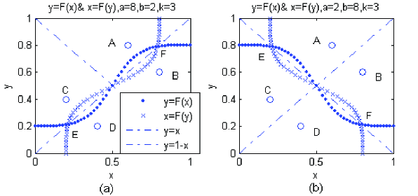
Figure 9: LBP updating function in (24) for $a>b$ and $a<b$.

This property conforms to the analysis of Mooij and Kappen (2005) and Watanabe and Fukumizu (2009). We will show the symmetry of fixed-point messages for uniform binary graphs as follows.

Property 3

For a completely uniform binary graph, synchronous LBP will either converge to the unique fixed point $\begin{pmatrix}0.5\\ 0.5\end{pmatrix}$ (paramagnetic fixed point), or converge to one of $\begin{pmatrix}x^{*}\\ 1-x^{*}\end{pmatrix}$ and $\begin{pmatrix}1-x^{*}\\ x^{*}\end{pmatrix}$ when $a>b$ (ferromagnetic), or oscillate between $\begin{pmatrix}x^{*}\\ 1-x^{*}\end{pmatrix}$ and $\begin{pmatrix}1-x^{*}\\ x^{*}\end{pmatrix}$ when $a<b$ (anti-ferromagnetic). When $a>b$, $x^{*}$ is the solution to $x^{*}=F(x^{*})$; otherwise, $x^{*}$ is the solution to $1-x^{*}=F(x^{*})$.

The proof appears in Appendix A.

From the previous property, we can conclude that completely uniform binary graphs will have at most second order periodicity. In other words, $F^{2n}(x)=x\Leftrightarrow F^{2}(x)=x$ and $F^{2n-1}(x)=x\Leftrightarrow F(x)=x$.

Let us calculate the fixed points and quasi-fixed points for the uniform graph in Fig. 3(c) with $a=\eta$ and $b=1-\eta$. Solving $x=\frac{\eta x^{3}+(1-\eta)(1-x)^{3}}{x^{3}+(1-x)^{3}}$ and $1-x=\frac{\eta x^{3}+(1-\eta)(1-x)^{3}}{x^{3}+(1-x)^{3}}$ yields the fixed points and quasi-fixed points respectively, for the graph in Fig. 3(c). Specifically, we can obtain four solutions of fixed points $\{\frac{1}{2},\frac{1}{2},\frac{-2+\eta-\sqrt{-4+8\eta-3\eta^{2}}}{2(-2+\eta)},\frac{-2+\eta+\sqrt{-4+8\eta-3\eta^{2}}}{2(-2+\eta)}\}$ and four solutions of quasi-fixed points $\{\frac{1}{2},\frac{1}{2},\frac{1+\eta-\sqrt{1-2\eta-3\eta^{2}}}{2(1+\eta)},\frac{1+\eta+\sqrt{1-2\eta-3\eta^{2}}}{2(1+\eta)}\}$. When $\eta>2/3$, the graph has two real fixed points except $0.5$; when $\eta<1/3$, the graph has two real quasi-fixed points except $0.5$; when $1/3<\eta<2/3$, the graph has one real fixed point $0.5$. For instance, when $\eta=0.7$, we have two stable fixed points $(0.9071,0.0929)$ and $(0.0929,0.9071)$; when $\eta=0.3$, we have two quasi-fixed points $(0.9071,0.0929)$ and $(0.0929,0.9071)$. We observe that both cases have the same strength of potential function $d(\psi)^{2}=0.7/0.3$, though their dynamic characteristics are different.

Based on Property 3, we find that for completely uniform graphs, the maximum multiplicative error and the minimum multiplicative error between two fixed-point messages are reciprocal. In other words, $d(e(x))=\max{e(x)}$. Therefore, compared to our uniform distance bound in Corollary 3, we have a tighter distance bound as follows.

Corollary 25

(Uniform Distance Bound for Completely Uniform Binary Graph)
$\mathbb{G}(\mathbb{V},\mathbb{E})$ is a completely uniform binary graphical model. The log-distance bound on beliefs at node $s$ is

$$\sum_{t\in\Gamma_{s}}\log\frac{d(\psi_{ts})^{2}\varepsilon+1}{d(\psi_{ts})^{2}+\varepsilon},$$

where $\varepsilon$ should satisfy

$$\log{\varepsilon}=\max_{(s,p)\in\mathbb{E}}\sum_{t\in\Gamma_{s}\backslash p}\log{\frac{d(\psi_{ts})^{2}\varepsilon+1}{d(\psi_{ts})^{2}+\varepsilon}}.$$

Proof  $\log\max E_{s}=\log d(E_{s})\leq\sum_{t\in\Gamma_{s}}\log d(e_{ts})\leq\sum_{t\in\Gamma_{s}}\log\frac{d(\psi_{ts})^{2}\varepsilon+1}{d(\psi_{ts})^{2}+\varepsilon}$.  
For the uniform graph in Fig. 3(c), when $\eta=0.7$, we have the true log-distance equal to $2.2785$, while our previous log-distance bound in Corollary 25 obtains $2.2785$, which is exactly equal to the true value, and our Improved-UDB in Corollary 7 obtains $2.3318$.

7.2 True Error-Variation Function

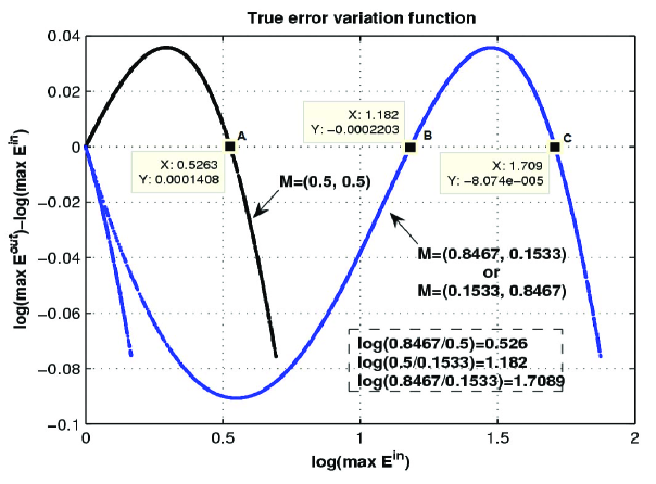
Figure 10: True error variation function when $M$s are fixed-point messages for the completely uniform graph in Fig. 3(c). $a=0.7$, $b=0.3$. The fixed-point messages are: $M=(0.8467,0.1533)$, $M=(0.1533,0.8467)$ and $M=(0.5,0.5)$.

In this section, we characterize the true error-variation function for a completely uniform binary graph. We have the following message updating equation:

$$\begin{pmatrix}me^{out}_{1}\\ (1-m)e^{out}_{2}\end{pmatrix}=\frac{1}{a+b}\begin{pmatrix}a&b\\ b&a\end{pmatrix}\begin{pmatrix}ME^{in}_{1}\\ (1-M)E^{in}_{2}\end{pmatrix},$$

where $M$ is the product of fixed-point incoming messages, $m$ is the fixed-point outgoing message, $E^{in}$ represents the product of incoming errors and $e^{out}$ represents the outgoing error. Assuming $E^{in}$ is the same for each node at a level on the Bethe tree, we have the following error equation:

$$\begin{pmatrix}E^{out}_{1}\\ E^{out}_{2}\end{pmatrix}=\frac{(aM+b(1-M))^{k}+(bM+a(1-M))^{k}}{(aME^{in}_{1}+b(1-M)E^{in}_{2})^{k}+(bME^{in}_{1}+a(1-M)E^{in}_{2})^{k}}\begin{pmatrix}\frac{(aME^{in}_{1}+b(1-M)E^{in}_{2})^{k}}{(aM+b(1-M))^{k}}\\ \frac{(bME^{in}_{1}+a(1-M)E^{in}_{2})^{k}}{(bM+a(1-M))^{k}}\end{pmatrix},$$

where $E^{out}$ is the product of outgoing errors flowing into a node at the upper level.

When $E^{in}_{1}>E^{in}_{2}$ and $a>b$, we have $E^{out}_{1}>E^{out}_{2}$. Therefore, letting $E$ denote $E^{in}_{1}$, we obtain the true error variation function:

$$G(log(E))=\log\max{E^{out}}-\log\max{E^{in}}$$

$$=\log{(\frac{(aME+b(1-ME))^{k}}{(aM+b(1-M))^{k}}\cdot\frac{(aM+b(1-M))^{k}+(bM+a(1-M))^{k}}{(aME+b(1-ME))^{k}+(bME+a(1-ME))^{k}})}-\log{E},$$ (25)

when $1<E<1/M$ and $a>b$.

An example of the true error variation function is illustrated in Fig. 10 for the graphical model in Fig. 3 (c). The curve of the error variation function $G(\log{E})$ in Equation (25) varies with the choice of $M$. The black curve corresponds to $G(\log{E})$ for $M=(0.5,0.5)$, while the blue curve corresponds to $G(\log{E})$ for $M=(0.8467,0.1533)$ or $M=(0.1533,0.8467)$. Since $G^{(1)}(\infty)=-1$, when $G(\log{E})$ does not cross the horizontal axis except the point at $\log{E}=0$, we have $G(\log{E})<0$ for $\log{E}>0$. In other words, $\log{E}$ will eventually decrease to zero and LBP converges to a unique fixed point. However, when $G(\log{E})$ crosses the horizontal axis besides $\log{E}=0$, $\log{E}$ will eventually stay at stable points, in which case, the product of the incoming errors at one level of Bethe tree equals the product of the incoming errors at its upper level. In other words, errors will not decrease after one LBP update. In Fig. 10, for the black curve, when $\log{E}$ leaves zero, it will eventually stay at $A$. For the blue curve in Fig. 10, when $\log{E}$ is between zero and the value at point $B$, it will decrease and finally stay at zero; when $\log{E}$ is bigger than the value at point $B$, it will increase and finally stay at point $C$. We can see that point $B$ is an unstable point.

From the example in Fig. 10, we can observe that the zero-crossing points of $\log{E}$ correspond to the exact log distances between two fixed-point messages. Specifically, the value at point $A$ is equal to the maximal log distance between $M=(0.8467,0.1533)$ and $M=(0.5,0.5)$, and the value at point $B$ is equal to the maximal log distance between $M=(0.5,0.5)$ and $M=(0.1533,0.8467)$, and the value at point $C$ is equal to the maximal log distance between $M=(0.8467,0.1533)$ and $M=(0.1533,0.8467)$. Therefore, our true error function in Equation (25) characterizes the true distance between fixed points, when LBP does not converge.

8 Conclusion

In this paper, we presented tighter error bounds on Loopy Belief Propagation (LBP) and used these bounds to study the dynamics—error, convergence, accuracy, and scheduling—of the sum-product algorithm. Specifically, we derived tight upper- and lower-bounds on error propagation in synchronous belief networks. We subsequently relied on these bounds to provide uniform and non-uniform distance bounds for the sum-product algorithm. We then used the distance bounds to obtain uniform and non-uniform sufficient conditions for convergence of the sum-product algorithm. We investigated the relation between convergence of LBP with sparsity and walk-summability of graphical models. We also showed that upper-bounds on message errors can be utilized to determine a priority for scheduling in sequential belief propagation. Moreover, we studied the accuracy of the bounds on the sum-product algorithm based on our error bounds. We also presented a case study of LBP by characterizing the dynamics of the sum-product algorithm for completely uniform graphs and analyzed its fixed and quasi-fixed (oscillatory) points.

Appendix A. Detailed Proofs

Proof of Theorem 1

Proof  We use maximum multiplicative error function as an error measure:

$$\max_{x_{s}}e^{i+1}_{ts}(x_{s})=\max_{x_{s}}\frac{\int\psi_{ts}(x_{t},x_{s})M_{ts}(x_{t})E^{i}_{ts}(x_{t})dx_{t}}{\int\psi_{t\star}(x_{t})M_{ts}(x_{t})E^{i}_{ts}(x_{t})dx_{t}}\times\frac{\int\psi_{t\star}(x_{t})M_{ts}(x_{t})dx_{t}}{\int\psi_{ts}(x_{t},x_{s})M_{ts}(x_{t})dx_{t}},$$

where $\psi_{t\star}(x_{t})=\int\psi_{ts}(x_{t},x_{s})dx_{s}$. The minimum multiplicative error function $\min_{x_{s}}e^{i+1}_{ts}(x_{s})$ is also used as an error measure in this theorem. Some assumptions throughout this proof are: $\psi_{ts}(x_{t},x_{s})$ is positive; message product $M_{ts}(x_{t})$ and polluted message product $M_{ts}(x_{t})E^{i}_{ts}(x_{t})$ are positive and normalized.

We use the same framework of proof as that in (Ihler et al., 2005, Thm. 8). Let us first introduce a lemma that will be used in our proof.

Lemma 26

For $f_{1},f_{2},g_{1},g_{2}$ all positive,

$$\frac{f_{1}+f_{2}}{g_{1}+g_{2}}\leq\max[\frac{f_{1}}{g_{1}},\frac{f_{2}}{g_{2}}],\quad\frac{f_{1}+f_{2}}{g_{1}+g_{2}}\geq\min[\frac{f_{1}}{g_{1}},\frac{f_{2}}{g_{2}}].$$

Proof  The left inequality is proved in Ihler et al. (2005). Let us restate it here. Assume without loss of generality that $f_{1}/g_{1}\geq f_{2}/g_{2}$ so that $f_{1}g_{2}\geq f_{2}g_{1}\Rightarrow f_{1}g_{2}+f_{1}g_{1}\geq f_{2}g_{1}+f_{1}g_{1}\Rightarrow\frac{f_{1}}{g_{1}}\geq\frac{f_{1}+f_{2}}{g_{1}+g_{2}}$. For the right inequality assume without loss of generality that $f_{1}/g_{1}\leq f_{2}/g_{2}$ so that $f_{1}g_{2}\leq f_{2}g_{1}\Rightarrow f_{1}g_{2}+f_{1}g_{1}\leq f_{2}g_{1}+f_{1}g_{1}\Rightarrow\frac{f_{1}}{g_{1}}\leq\frac{f_{1}+f_{2}}{g_{1}+g_{2}}$.  

Similar to the analysis in (Ihler et al., 2005, Lemma 26),we need the following lemma to assist our proof. In the following, we shall omit reference to the iteration number of the messages and errors for simplicity and clarity of the presentation.

Lemma 27

The maximum of $\max_{x_{s}}e_{ts}(x_{s})$ or the minimum of $\min_{x_{s}}e_{ts}(x_{s})$ is attained when

$$\psi_{ts}(x_{t},x_{s})=1+(d(\psi_{ts})^{2}-1)\chi_{\psi}(x_{t}),\quad\psi_{t\star}(x_{t})=1+(d(\psi_{t\star})^{2}-1)\chi_{\star}(x_{t})$$

$$E_{ts}(x_{t})=1+(d(E_{ts})^{2}-1)\chi_{E}(x_{t}),$$

where $\chi_{\psi}$, $\chi_{\star}$ and $\chi_{E}$ are indicator functions.

Proof  Let $\psi_{ts}(x_{t},x_{s})=\alpha_{1}\psi_{1}(x_{t},x_{s})+\alpha_{2}\psi_{2}(x_{t},x_{s})$,where $\alpha_{1}\geq 0$,$\alpha_{2}\geq 0$, $\alpha_{1}+\alpha_{2}=1$. In other words,$\psi_{ts}(x_{t},x_{s})$ is a convex combination of two arbitrary positive functions $\psi_{1}(x_{t},x_{s})$ and $\psi_{2}(x_{t},x_{s})$. Thus, by applying Lemma 26, we have:

$$\frac{\alpha_{1}\int\psi_{1}(x_{t},x_{s})M_{ts}(x_{t})E_{ts}(x_{t})dx_{t}+\alpha_{2}\int\psi_{2}(x_{t},x_{s})M_{ts}(x_{t})E_{ts}(x_{t})dx_{t}}{\alpha_{1}\int\psi_{1}(x_{t},x_{s})M_{ts}(x_{t})dx_{t}+\alpha_{2}\int\psi_{2}(x_{t},x_{s})M_{ts}(x_{t})dx_{t}}$$

$$\leq\max[\frac{\int\psi_{1}(x_{t},x_{s})M_{ts}(x_{t})E_{ts}(x_{t})dx_{t}}{\int\psi_{1}(x_{t},x_{s})M_{ts}(x_{t})dx_{t}},\frac{\int\psi_{2}(x_{t},x_{s})M_{ts}(x_{t})E_{ts}(x_{t})dx_{t}}{\int\psi_{2}(x_{t},x_{s})M_{ts}(x_{t})dx_{t}}].$$

We find that $\max_{x_{s}}e_{ts}(x_{s})$ is maximized when we take the maximum of the RHS expression in the previous inequality. Let us scale $\psi_{ts}(x_{t},x_{s})$ so that the minimal value of the function is $1$. Thus, $\psi_{ts}(x_{t},x_{s})$ can be composed by a convex combination of functions which have the form $1+(d(\psi_{ts})^{2}-1)\chi_{\psi}(x_{t})$, where $\chi_{\psi}(x_{t})$ is an indicator function. We can find that the $\max_{x_{s}}e_{ts}(x_{s})$ is maximized when $\psi_{ts}(x_{t},x_{s})=1+(d(\psi_{ts})^{2}-1)\chi_{\psi}(x_{t})$. Similar are the proofs for $\psi_{t\star}(x_{t})$ and $E_{ts}(x_{t})$.

To minimize the $\min_{x_{s}}e_{ts}(x_{s})$, by applying Lemma 26, we have:

$$\frac{\alpha_{1}\int\psi_{1}(x_{t},x_{s})M_{ts}(x_{t})E_{ts}(x_{t})dx_{t}+\alpha_{2}\int\psi_{2}(x_{t},x_{s})M_{ts}(x_{t})E_{ts}(x_{t})dx_{t}}{\alpha_{1}\int\psi_{1}(x_{t},x_{s})M_{ts}(x_{t})dx_{t}+\alpha_{2}\int\psi_{2}(x_{t},x_{s})M_{ts}(x_{t})dx_{t}}$$

$$\geq\min[\frac{\int\psi_{1}(x_{t},x_{s})M_{ts}(x_{t})E_{ts}(x_{t})dx_{t}}{\int\psi_{1}(x_{t},x_{s})M_{ts}(x_{t})dx_{t}},\frac{\int\psi_{2}(x_{t},x_{s})M_{ts}(x_{t})E_{ts}(x_{t})dx_{t}}{\int\psi_{2}(x_{t},x_{s})M_{ts}(x_{t})dx_{t}}].$$

Furthermore, by constructing the potential function $\psi_{ts}(x_{t},x_{s})$ as a convex combination of functions of the form $1+(d(\psi_{ts})^{2}-1)\chi_{\psi}(x_{t})$, where $\chi_{\psi}(x_{t})$ is an indicator function, we can find that $\min_{x_{s}}e_{ts}(x_{s})$ is minimized when $\psi_{ts}(x_{t},x_{s}))$ is one of these functions. Similar are the proofs for $\psi_{t\star}(x_{t})$ and $E_{ts}(x_{t})$.  
So we have $\max_{x_{s}}e_{ts}(x_{s})$ is bounded by

$$\frac{\int\psi_{ts}(x_{t},x_{s})M_{ts}(x_{t})E_{ts}(x_{t})dx_{t}}{\int\psi_{t\star}(x_{t})M_{ts}(x_{t})E_{ts}(x_{t})dx_{t}}\times\frac{\int\psi_{t\star}(x_{t})M_{ts}(x_{t})dx_{t}}{\int\psi_{ts}(x_{t},x_{s})M_{ts}(x_{t})dx_{t}}$$

$$=\frac{\int(1+(d(\psi_{ts})^{2}-1)\chi_{\psi}(x_{t}))M_{ts}(x_{t})(1+(d(E_{ts})^{2}-1)\chi_{E}(x_{t}))dx_{t}}{\int(1+(d(\psi_{t\star})^{2}-1)\chi_{\star}(x_{t}))M_{ts}(x_{t})(1+(d(E_{ts})^{2}-1)\chi_{E}(x_{t}))dx_{t}}$$

$$\times\frac{\int(1+(d(\psi_{t\star})^{2}-1)\chi_{\star}(x_{t}))M_{ts}(x_{t})dx_{t}}{\int(1+(d(\psi_{ts})^{2}-1)\chi_{\psi}(x_{t}))M_{ts}(x_{t})dx_{t}}.$$

Define the quantities:

$$M_{A}=\int M_{ts}(x_{t})\chi_{\psi}(x_{t})dx_{t},\quad M_{B}=\int M_{ts}(x_{t})\chi_{\star}(x_{t})dx_{t},\quad M_{E}=\int M_{ts}(x_{t})\chi_{E}(x_{t})dx_{t},$$

$$M_{AE}=\int M_{ts}(x_{t})\chi_{\psi}(x_{t})\chi_{E}(x_{t})dx_{t},\quad M_{BE}=\int M_{ts}(x_{t})\chi_{\star}(x_{t})\chi_{E}(x_{t})dx_{t},$$

$$\alpha_{1}=d(\psi_{ts})^{2}-1,\quad\alpha_{2}=d(\psi_{t\star})^{2}-1,\quad\beta=d(E_{ts})^{2}-1.$$

The maximum multiplicative error $\max_{x_{s}}e_{ts}(x_{s})$ is upper-bounded by $\Delta_{1}$ where

$$\Delta_{1}=\max_{M}\frac{1+\alpha_{1}M_{A}+\beta M_{E}+\alpha_{1}\beta M_{AE}}{1+\alpha_{2}M_{B}+\beta M_{E}+\alpha_{2}\beta M_{BE}}\,\frac{1+\alpha_{2}M_{B}}{1+\alpha_{1}M_{A}}.$$

The maximum is obtained when $M_{AE}=M_{A}=M_{E}=1-M_{B}$ and $M_{BE}=0$, which gives

$$\Delta_{1}=\max_{M_{E}}\frac{1+(\alpha_{1}+\beta+\alpha_{1}\beta)M_{E}}{1+\alpha_{2}+(\beta-\alpha_{2})M_{E}}\,\frac{1+\alpha_{2}-\alpha_{2}M_{E}}{1+\alpha_{1}M_{E}}.$$

Taking the derivative wrt $M_{E}$ and setting it to zero, we obtain

$$\max_{x_{s}}e_{ts}(x_{s})\leq\Delta_{1}=\left(\frac{d(\psi_{ts})d(\psi_{t\star})d(E_{ts})+1}{d(\psi_{ts})d(\psi_{t\star})+d(E_{ts})}\right)^{2}.$$

Similarly to what we have done so far, we can lower-bound $\min_{x_{s}}e_{ts}(x_{s})$ with respect to $\psi_{ts}(x_{t},x_{s})$, $\psi_{t\star}(x_{t})$ and $E_{ts}(x_{t})$, to obtain

$$\min_{x_{s}}e_{ts}(x_{s})\geq\left(\frac{d(\psi_{ts})d(\psi_{t\star})+d(E_{ts})}{d(\psi_{ts})d(\psi_{t\star})d(E_{ts})+1}\right)^{2}=\frac{1}{\Delta_{1}}.$$

 
Proof of Corollary 3

Proof  Let $\Delta_{ut}(x)=(\frac{d(\psi_{ut})d(\psi_{u\star})x+1}{d(\psi_{ut})d(\psi_{u\star})+x})^{2},x\geq 1,ut\in\mathbb{E}$. Therefore,

$$d(E_{ts}^{i})\leq\prod_{u\in\Gamma_{t}\backslash s}d(e_{ut}^{i})=\prod_{u\in\Gamma_{t}\backslash s}\frac{\max\sqrt{e_{ut}^{i}(x_{t})}}{\min\sqrt{e_{ut}^{i}(x_{t})}}\leq\varepsilon_{ts}^{i}=\prod_{u\in\Gamma_{t}\backslash s}\Delta_{ut}(d(E_{ut}^{i-1})).$$

Thus, we have

$$\max_{x_{s}}E_{sp}^{i+1}(x_{s})\leq\prod_{t\in\Gamma_{s}\backslash p}\max_{x_{s}}e_{ts}^{i+1}(x_{s})\leq\varepsilon_{sp}^{i+1}=\prod_{t\in\Gamma_{s}\backslash p}\Delta_{ts}(d(E_{ts}^{i}))$$

$$\leq\prod_{t\in\Gamma_{s}\backslash p}\Delta_{ts}(\varepsilon_{ts}^{i})\leq\prod_{t\in\Gamma_{s}\backslash p}\Delta_{ts}(\max_{t\in\Gamma_{s}\backslash p}\varepsilon_{ts}^{i})=\Delta_{3}(\max_{t\in\Gamma_{s}\backslash p}\varepsilon_{ts}^{i}).$$

The term $\varepsilon_{sp}^{i+1}$ is an upper-bound on the incoming error product $E_{sp}^{i+1}(x_{s})$ at iteration $i+1$, while $\max_{t\in\Gamma_{s}\backslash p}\varepsilon_{ts}^{i}$ is the maximum of the upper-bounds on the incoming error products $\{E_{ts}^{i}(x_{t}),t\in\Gamma_{s}\backslash p\}$ at iteration $i$. We hope to achieve that $\varepsilon_{sp}^{i+1}<\max_{t\in\Gamma_{s}\backslash p}\varepsilon_{ts}^{i}$. Denoting $\varepsilon=\max_{t\in\Gamma_{s}\backslash p}\varepsilon_{ts}^{i}$, let us introduce an error bound-variation function:

$$G_{sp}(\log{\varepsilon})=\log\Delta_{3}(\varepsilon)-\log{\varepsilon}\geq\log\varepsilon_{sp}^{i+1}-\log\max_{t\in\Gamma_{s}\backslash p}\varepsilon_{ts}^{i},\varepsilon\geq 1,$$

which describes variation of error bound after each iteration. When $G_{sp}(\log{\varepsilon})=0$, the log-distance bound $\log{\varepsilon}$ will reach a fixed point, which is the maximal distance between message products at various iterations. Because $G_{sp}^{(2)}(\log{\varepsilon})<0$ for $\log{\varepsilon}>0$ and $G_{sp}^{(1)}(\infty)=-1/2$, $G_{sp}^{(1)}(\log{\varepsilon})$ will decrease until it is equal to $-1/2$. Therefore, it only has one crossing point besides $\log{\varepsilon}=0$ (zero crossing point). This nonzero crossing point is a stable fixed point of function $G_{sp}(\log{\varepsilon})$. In other words, once $\log{\varepsilon}$ leaves the zero crossing point, it will stay at this stable crossing point, $\log{\varepsilon^{*}}$, which corresponds to the upper bound on error products.

Because the distance between fixed points of $B_{s}(x_{s})$ is

$$\log{E_{s}(x_{s})}=\log{\prod_{t\in\Gamma_{s}}e_{ts}(x_{s})}\leq\log{\prod_{t\in\Gamma_{s}}\Delta_{ts}(\varepsilon^{*})},$$

we can obtain the log-distance bound on $B_{s}(x_{s})$ by taking the maximum $\varepsilon^{*}$.  
Proof of Theorem 4

Proof  Let us revisit the error bound-variation function in Equation (14):

$$G_{sp}(\log{\varepsilon})=\log{\prod_{t\in\Gamma_{s}\backslash p}(\frac{d(\psi_{ts})d(\psi_{t\star})\varepsilon+1}{d(\psi_{ts})d(\psi_{t\star})+\varepsilon}})^{2}-\log{\varepsilon},$$

which describes the variation of the error bound after each iteration. To guarantee that LBP converges, it is sufficient to require $G_{sp}(\log{\varepsilon})<0,\forall\log{\varepsilon}>0$. Let $z=\log{\varepsilon}$. The second derivative of $G_{sp}(z)$ is

$$G_{sp}^{(2)}(z)=2\times\sum_{t\in\Gamma_{s}\backslash p}\frac{d(\psi_{ts})d(\psi_{t\star})e^{z}((d(\psi_{ts})d(\psi_{t\star}))^{2}-1)(1-e^{2z})}{(d(\psi_{ts})d(\psi_{t\star})e^{z}+1)^{2}(d(\psi_{ts})d(\psi_{t\star})+e^{z})^{2}}\leq 0,$$

when $d(\psi_{ts})d(\psi_{t\star})>1$ and $z\geq 0$. When $z>0$, $G_{sp}(z)$ is strictly concave.

The first derivation of $G_{sp}(z)$ is

$$G_{sp}^{(1)}(z)=2\times\sum_{t\in\Gamma_{s}\backslash p}\frac{e^{z}((d(\psi_{ts})d(\psi_{t\star}))^{2}-1)}{(d(\psi_{ts})d(\psi_{t\star})e^{z}+1)(d(\psi_{ts})d(\psi_{t\star})+e^{z})}-1.$$

Because $G_{sp}(z=0)=0$, if the first derivative $G_{sp}^{(1)}(z=0)<0$, we will have $G_{sp}(z>0)<0$. Therefore,

$$G_{sp}^{(1)}(0)=2\times\sum_{t\in\Gamma_{s}\backslash p}\frac{((d(\psi_{ts})d(\psi_{t\star}))^{2}-1)}{(d(\psi_{ts})d(\psi_{t\star})+1)(d(\psi_{ts})d(\psi_{t\star})+1)}-1<0$$

$$\Rightarrow\sum_{t\in\Gamma_{s}\backslash p}\frac{d(\psi_{ts})d(\psi_{t\star})-1}{d(\psi_{ts})d(\psi_{t\star})+1}<\frac{1}{2}.$$

 
Proof of Theorem 9

Proof  Recall that in the proof of uniform convergence condition, we use an error bound-variation function $G_{sp}(\log{\varepsilon})$, which is originally to describe $(\log{\varepsilon_{sp}^{i+1}}-\log{\varepsilon_{ts}^{i}})$, for $\forall(s,p)\in\mathbb{E}$. For each $T(\mathbb{G},v)$, given $vu\in\mathbb{\bar{E}}$, let us introduce the following error bound-variation function:

$$G_{vu}(\{\log{\varepsilon_{w_{i}v}}\},\log{\varepsilon})=\sum_{w_{i}\in\Gamma_{v}\backslash u}\log{\frac{d(\psi_{l(w_{i})v})^{2}\varepsilon_{w_{i}v}+1}{d(\psi_{l(w_{i})v})^{2}+\varepsilon_{w_{i}v}}}-\log{\varepsilon},$$

$$\log{\varepsilon_{w_{i}v}}=\sum_{w_{j}\in\Gamma_{w_{i}}\backslash v}\log{\frac{d(\psi_{l(w_{j})l(w_{i})})^{2}\varepsilon_{w_{j}w_{i}}+1}{d(\psi_{l(w_{j})l(w_{i})})^{2}+\varepsilon_{w_{j}w_{i}}}},$$

$$...$$

$$\log{\varepsilon_{w_{q}w_{p}}}=\sum_{w_{r}\in\Gamma_{w_{q}}\backslash w_{p}}\log{\frac{d(\psi_{l(w_{r})l(w_{q})})^{2}\varepsilon+1}{d(\psi_{l(w_{r})l(w_{q})})^{2}+\varepsilon}},$$

where $\{w_{r}\}$ is the set of leaf nodes of $T(\mathbb{G},v)$.

To guarantee LBP to converge, it is sufficient to have $G_{vu}(\log{\varepsilon})<0$ for $\forall\log{\varepsilon}>0$. Because $G_{vu}(\log{\varepsilon}=0)=0$, when $G_{vu}^{\prime}(\log{\varepsilon}=0)<0$, we will definitely have $G_{vu}(0<\log{\varepsilon}<\delta)<0$, where $\delta$ is a small positive value. When $G_{vu}(\log{\varepsilon})$ is concave, $\delta$ can be infinity so that the convergence of LBP is true for $\forall\log{\varepsilon}>0$. However, because $G_{vu}(\log{\varepsilon})$ is not guaranteed to be concave, we will only obtain local convergence for an infinitesimal $\delta$.

Define $f_{w_{j}w_{i}}(\varepsilon_{w_{j}w_{i}})=\log{\frac{d(\psi_{l(w_{j})l(w_{i})})^{2}\varepsilon_{w_{j}w_{i}}+1}{d(\psi_{l(w_{j})l(w_{i})})^{2}+\varepsilon_{w_{j}w_{i}}}}$. Thus, we have the first derivative of
$G_{vu}(\{\log{\varepsilon_{w_{i}v}}\},\log{\varepsilon})$ as follows:

$$\frac{\partial G_{vu}(\{\log{\varepsilon_{w_{i}v}}\},\log{\varepsilon})}{\partial\log{\varepsilon}}=\sum_{w_{i}\in\Gamma_{v}\backslash u}f_{w_{i}v}^{\prime}\sum_{w_{j}\in\Gamma_{w_{i}}\backslash v}f_{w_{j}w_{i}}^{\prime}....\sum_{w_{r}\in\Gamma_{w_{q}}\backslash w_{p}}f_{w_{r}w_{q}}^{\prime}-1,$$

where $f^{\prime}=\frac{\partial f(\log{\varepsilon})}{\partial\log{\varepsilon}}=\frac{(d(\psi)^{4}-1)\varepsilon}{(d(\psi)^{2}\varepsilon+1)(d(\psi)^{2}+\varepsilon)}$. Plugging $\log{\varepsilon}=0$ into the previous equation, we obtain our non-uniform convergence condition.  
Proof of Property 3

Proof  Let us analyze the fixed points by solving the set of equations

$$y=F(x)$$ (26a)

$$x=F(y)$$ (26b)

which corresponds to second order periodicity $x=F^{2}(x)$. The set of equations is depicted in Fig. 9 for $a>b$ and $a<b$ respectively. We can easily find that $F(x)$ and $F(y)$ are symmetric with respect to $y=x$. Moreover, because $F(x)$ is symmetric about the point $(0.5,0.5)$, we have $F(1-x)=1-F(x)$. Therefore, it is easy to see that $F(x)$ and $F(y)$ are also symmetric with respect to $y=1-x$. Let us check whether the two functions are symmetric with respect to other lines such as $y=\beta+\alpha x$. Substitute $y=\beta+\alpha x$ and $x=\frac{1}{\alpha}(y-\beta)$ in (26a). We have $\beta+\alpha x=\frac{a(y-\beta)^{k}+b(\alpha-(y-\beta))^{k}}{(a+b)((y-\beta)^{k}+(\alpha-(y-\beta))^{k})}$. For this equation to be always equivalent to (26b), we have $(\alpha=1,\beta=0)$ or $(\alpha=-1,\beta=1)$. Thus, the set of equations is only symmetric with respect to $y=x$ and $y=1-x$.

When $y=F(x)$ and $x=F(y)$ intersect, they must have crossing points on $y=x$ or $y=1-x$. In the following, we will show that they do not cross elsewhere. When $a>b$, let us assume these two functions have one crossing point A not on $y=x$ and $y=1-x$, which is illustrated in Fig. 9 (a). Due to the symmetry between $F(x)$ and $F(y)$, they must have the other three crossing points $B,C$ and $D$ shown in Fig. 9 (a) respectively. Both functions must go through those points. The first derivative of $F(x)$ is $F^{(1)}(x)=\frac{k(a-b)x^{k-1}(1-x)^{k-1}}{(a+b)((1-x)^{k}+x^{k})^{2}}=\left\{\begin{array}[]{c}>0,a>b\\ <0,a<b\end{array}\right.$, which shows that function $F(x)$ is either monotonic increasing or monotonic decreasing. Because $y_{B}<y_{A}$, when $x_{B}>x_{A}$, we arrive at a contradiction with the monotonic increasing property under the condition $a>b$. Similar result is for $a<b$. According to Property 2, $y=F(x)$ and $x=F(y)$ have at most three real crossings points with an arbitrary line. Therefore, we can see that the set of equations will have at most three crossing points with either $y=x$ or $y=1-x$.

The set of equations in (26a) and (26b) has a naive fixed point $(0.5,0.5)$. However, it is only stable when the set of equations crosses nowhere else on $y=x$ and $y=1-x$. When $a>b$ and $F^{(1)}(\frac{1}{2})=\frac{k(a-b)}{(a+b)}>1$, we can see that the belief network will either converge at fixed point E or at fixed point F on $y=x$ in Fig.9 (a). In this case, the fixed point at $x=0.5$ is an unstable point. When $a<b$ and $F^{(1)}(\frac{1}{2})<-1$, the belief network will eventually oscillate between E and F on $y=1-x$, which is shown in Fig. 9 (b). The fixed point at $x=0.5$ is again an unstable fixed point. Because $F(x)$ is symmetric with respect to $(x=0.5,y=0.5)$, points E and F are symmetric with respect to $(x=0.5,y=0.5)$.

References

- Bishop (2006) C.M. Bishop. Pattern Recognition and Machine Learning (Information Science and Statistics). Springer, 2006.
- Elidan et al. (2006) Gal Elidan, Ian Mcgraw, and Daphne Koller. Residual belief propagation: informed scheduling for asynchronous message passing. In Uncertainty in Artificial Intellignece, 2006.
- Georgii (1988) Hans-Otto Georgii. Gibbs Measures and Phase Transitions. Walter de Gruyter and Co., 1988.
- Heskes (2004) Tom Heskes. On the uniqueness of loopy belief propagation fixed points. Neural Computation, 16:2379–2413, 2004.
- Ihler et al. (2005) A. T. Ihler, J. W. Fisher III, and A. S. Willsky. Loopy belief propagation: Convergence and effects of message errors. Journal of Machine Learning Research, 6:905–936, May 2005.
- Ihler (2007) Alexander Ihler. Accuracy bounds for belief propagation. In Proceedings of UAI 2007, July 2007.
- Jordan (1999) M. I. Jordan. Learning in Graphical Models. Mit Press, Boston, 1999.
- Kschischang et al. (2001) Frank R. Kschischang, Brendan J. Frey, and Hans-Andrea Loeliger. Factor graphs and the sum-product algorithm. IEEE Transactions on Information Theory, 47:498–519, 2001.
- Malioutov et al. (2006) Dmitry M. Malioutov, Jason K. Johnson, and Alan S. Willsky. Walk-sums and belief propagation in gaussian graphical models. J. Mach. Learn. Res., 7:2031–2064, 2006.
- Mceliece et al. (1998) Robert J. Mceliece, David J. C. Mackay, and Jung-fu Cheng. Turbo decoding as an instance of Pearl’s belief propagation algorithm. IEEE Journal on Selected Areas in Communications, pages 140–152, 1998.
- Mooij and Kappen (2005) J. M. Mooij and H. J. Kappen. On the properties of the Bethe approximation and loopy belief propagation on binary networks. Journal of Statistical Mechanics: Theory and Experiment, 2005(11):P11012, 2005.
- Mooij and Kappen (2007) J. M. Mooij and H. J. Kappen. Sufficient conditions for convergence of the sum-product algorithm. IEEE Transactions on Information Theory, 53(12):4422–4437, December 2007.
- (13) Joris M Mooij and Hilbert J Kappen. Bounds on marginal probability distributions. In Advances in Neural Information Processing Systems 21 (NIPS*2008).
- Ruozzi and Tatikonda (2010) Nicholas Ruozzi and Sekhar Tatikonda. Convergent and correct message passing schemes for optimization problems over graphical models. In Proceedings of the Twenty-Sixth Conference Annual Conference on Uncertainty in Artificial Intelligence (UAI-10), pages 500–500, 2010.
- Salas and Sokal (1997) Jesus Salas and Alan Sokal. Absence of phase transition for antiferromagnetic potts models via the dobrushin uniqueness theorem. Journal of Statistical Physics, 86:551–579, 1997.
- Shi et al. (2010) Xiangqiong Shi, Dan Schonfeld, and Daniela Tuninetti. Message error propagation for belief propagation. In 2010 IEEE International Conference on Acoustics, Speech, and Signal Processing (ICASSP), 2010.
- Sun et al. (2003) Jian Sun, Heung yeung Shum, and Nan ning Zheng. Stereo matching using belief propagation. IEEE Transactions on Pattern Analysis and Machine Intelligence, 25:787–800, 2003.
- Sutton and Mccallum (2007) Charles Sutton and Andrew Mccallum. Improved dynamic schedules for belief propagation. In Conference on Uncertainty in Artificial Intelligence (UAI), 2007.
- Taga and Mase (2006a) Nobuyuki Taga and Shigeru Mase. Error bounds between marginal probabilities and beliefs of loopy belief propagation algorithm. In MICAI, pages 186–196, 2006a.
- Taga and Mase (2006b) Nobuyuki Taga and Shigeru Mase. On the convergence of loopy belief propagation algorithm for different update rules. IEICE Transactions, 89-A(2):575–582, 2006b.
- Tatikonda (2003) S.C. Tatikonda. Convergence of the sum-product algorithm. In Information Theory Workshop, 2003. Proceedings. 2003 IEEE, pages 222–225, March-4 April 2003.
- Tatikonda and Jordan (2002) Sekhar Tatikonda and Michael I. Jordan. Loopy belief propogation and gibbs measures. In UAI, pages 493–500, 2002.
- Wainwright and Jordan (2008) M. J. Wainwright and M. I. Jordan. Graphical models, exponential families, and variational inference. Foundations and Trends in Machine Learning, 1:1–305, 2008.