Annotation

Currently there is a common belief that the explanation of superconductivity phenomenon lies in understanding the mechanism of the formation of electron pairs. Paired electrons, however, cannot form a superconducting condensate spontaneously. These paired electrons perform disorderly zero-point oscillations and there are no force of attraction in their ensemble. In order to create a unified ensemble of particles, the pairs must order their zero-point fluctuations so that an attraction between the particles appears. As a result of this ordering of zero-point oscillations in the electron gas, superconductivity arises. This model of condensation of zero-point oscillations creates the possibility of being able to obtain estimates for the critical parameters of elementary superconductors, which are in satisfactory agreement with the measured data. On the another hand, the phenomenon of superfluidity in He-4 and He-3 can be similarly explained, due to the ordering of zero-point fluctuations. It is therefore established that both related phenomena are based on the same physical mechanism.

Boris V.Vasiliev

SUPERCONDUCTIVITY
and
SUPERFLUIDITY

1 Superconductivity and zero-point oscillations

1.1 Superconductivity as a consequence of ordering of zero-point oscillations in electron gas

1.1.1 Superconductivity and superfluidity

Superfluidity and superconductivity, which can be regarded as the superfluidity of the electron gas, are related phenomena. The main feature of these phenomena can be seen in a fact that a special condensate in superconductors as well as in superfluid helium is formed from particles interconnected by attraction. This mutual attraction does not allow a scattering of individual particles on defects and walls, if the energy of this scattering is less than the energy of attraction. Due to the lack of scattering condensate acquires ability to move without friction.

Superconductivity was discovered over a century ago, and the superfluidity about thirty years later.

However, despite the attention of many scientists to the study of these phenomena, they have been the great mysteries in condensed matter physics for a long time. This mystery attracted the best minds of the twentieth century.

The mystery of the superconductivity phenomenon has begun to drop in the middle of the last century when the effect of magnetic flux quantization in superconducting cylinders was discovered and investigated. This phenomenon was predicted even before the WWII by brothers F. London and H. London, but its quantitative study were performed only two decades later.

By these measurements it became clear that at the formation of the superconducting state, two free electrons are combined into a single boson with zero spin and zero pulse.

Around the same time, it was observed that the substitution of one isotope of the superconducting element to another leads to a changing of the critical temperature of superconductors: the phenomenon called an isotope-effect [1], [2]. This effect was interpreted as the direct proof of the key role of phonons in the formation of the superconducting state.

Following these understandings, L. Cooper proposed the phonon mechanism of electron pairing on which base the microscopic theory of superconductivity (so called BCS-theory) was built by N. Bogolyubov and J. Bardin, L. Cooper and J. Shriffer (probably it should be named better the Bogolyubov-BCS-theory).

However the B-BCS theory based on the phonon mechanism brokes a hypothetic link between superconductivity and superfluidity as in liquid helium there are no phonons for combining atoms.

Something similar happened with the description of superfluidity.

Soon after discovery of superfluidity, L.D. Landau in his first papers on the subject immediately demonstrated that this phenomenon should be considered as a result of condensate formation consisting of macroscopic number of atoms in the same quantum state and obeying quantum laws. It gave the possibility to describe the main features of this phenomenon: the temperature dependence of the superfluid phase density, the existence of the second sound, etc. But it does not gave an answer to the question which physical mechanism leads to the unification of the atoms in the superfluid condensate and what is the critical temperature of the condensate, i.e. why the ratio of the temperature of transition to the superfluid state to the boiling point of helium-4 is almost exactly equals to $1/2$, while for helium-3, it is about a thousand times smaller.

On the whole, the description of both super-phenomena, superconductivity and superfluidity, to the beginning of the twenty first century induced some feeling of dissatisfaction primarily due to the fact that a common mechanism of their occurrence has not been understood.

More than fifty years of a study of the B-BCS-theory has shown that this theory successfully describes the general features of the phenomenon, but it can not be developed in the theory of superconductors. It explains general laws such as the emergence of the energy gap, the behavior of specific heat capacity, the flux quantization, etc., but it can not predict the main parameters of the individual superconductors: their critical temperatures and critical magnetic fields. More precisely, in the B-BCS-theory, the expression for the critical temperature of superconductor obtains an exponential form which exponential factor is impossible to measure directly and this formula is of no practical interest.

Recent studies of the isotopic substitution showed that zero-point oscillations of the ions in the metal lattice are not harmonical. Consequently the isotopic substitution affects the interatomic distances in a lattice, and as the result, they directly change the Fermi energy of a metal [3].

Therefore, the assumption developed in the middle of the last century, that the electron-phonon interaction is the only possible mechanism of superconductivity was proved to be wrong. The direct effect of isotopic substitution on the Fermi energy gives a possibility to consider the superconductivity without the phonon mechanism.

Furthermore, a closer look at the problem reveals that the B-BCS-theory describes the mechanism of electron pairing, but in this theory there is no mechanism for combining pairs in the single super-ensemble. The necessary condition for the existence of superconductivity is formation of a unique ensemble of particles. By this mechanism, a very small amount of electrons are combined in super-ensemble, on the level 10 in minus fifth power from the full number of free electrons. This fact also can not be understood in the framework of the B-BCS theory.

At very low temperatures, that allow superfluidity in helium and superconductivity in metals, all movements of particles are freezed except for their zero-point oscillations. Therefore, as an alternative, we should consider the interaction of super-particles through electro-magnetic fields of zero-point oscillations. This approach was proved to be fruitful. At the consideration of super-phenomena as consequences of the zero-point oscillations ordering, one can construct theoretical mechanisms enabling to give estimations for the critical parameters of these phenomena which are in satisfactory agreement with measurements.

As result, one can see that as the critical temperatures of (type-I) superconductors are equal to about $10^{-6}$ from the Fermi temperature for superconducting metal, which is consistent with data of measurements. At this the destruction of superconductivity by application of critical magnetic field occurs when the field destroys the coherence of zero-point oscillations of electron pairs. This is in good agreement with measurements also.

A such-like mechanism works in superfluid liquid helium. The problem of the interaction of zero-point oscillations of the electronic shells of neutral atoms in the s-state, was considered yet before the WWII by F.London. He has shown that this interaction is responsible for the liquefaction of helium. The closer analysis of interactions of zero-point oscillations for helium atomic shells shows that at first at the temperature of about 4K only one of the oscillations mode becomes ordered. As a result, the forces of attraction appear between atoms which are need for helium liquefaction. To create a single quantum ensemble, it is necessary to reach the complete ordering of atomic oscillations. At the complete ordering of oscillations at about 2K, the additional energy of the mutual attraction appears and the system of helium-4 atoms transits in superfluid state. To form the superfluid quantum ensemble in Helium-3, not only the zero-point oscillations should be ordered, but the magnetic moments of the nuclei should be ordered too. For this reason, it is necessary to lower the temperature below 0.001K. This is also in agreement with experiment.

Thus it is possible to show that both related super-phenomena, superconductivity and superfluidity, are based on the single physical mechanism: the ordering of zero-point oscillations.

The roles of zero-point oscillations in formation of the superconducting state have been previously considered in papers [4]-[6].

1.1.2 The electron pairing

J.Bardeen was first who turned his attention toward a possible link between superconductivity and zero-point oscillations [7].

The special role of zero-point vibrations exists due to the fact that at low temperatures all movements of electrons in metals have been freezen except for these oscillations.

Superconducting condensate formation requires two mechanisms: first, the electrons must be united in boson pairs, and then the zero-point fluctuations must be ordered (see Fig.(1)).

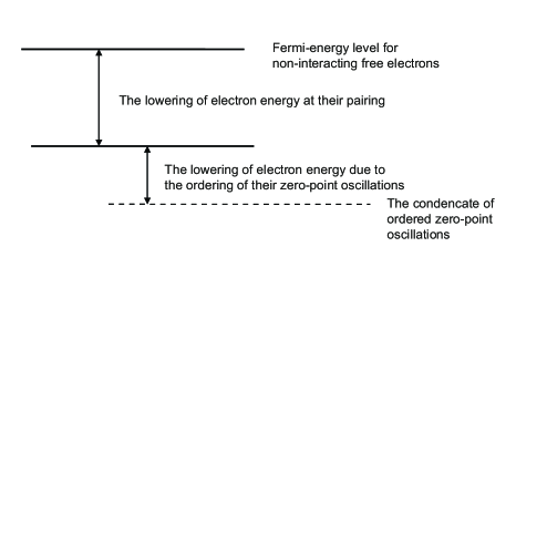
Figure 1: The schematic representation of the energy levels of conducting electrons in a superconducting metal

The energetically favorable pairing of electrons in the electron gas should occur above the critical temperature.

Possibly, the pairing of electrons can occur due to the magnetic dipole-dipole interaction.

For the magnetic dipole-dipole interaction, to merge two electrons into the singlet pair at the temperature of about 10K, the distance between these particles must be small enough:

$$r<(\mu_{B}^{2}/kT_{c})^{1/3}\approx a_{B},$$ (1)

where $a_{B}=\frac{\hbar^{2}}{m_{e}e^{2}}$ is the Bohr radius.

That is, two collectivized electrons must be localized in one lattice site volume. It is agreed that the superconductivity can occur only in metals with two collectivized electrons per atom, and cannot exist in the monovalent alkali and noble metals.

It is easy to see that the presence of magnetic moments on ion sites should interfere with the magnetic combination of electrons. This is confirmed by the experimental fact: as there are no strong magnetic substances among superconductors, so adding of iron, for example, to traditional superconducting alloys always leads to a lower critical temperature.

On the other hand, this magnetic coupling should not be destroyed at the critical temperature. The energy of interaction between two electrons, located near one lattice site, can be much greater. This is confirmed by experiments showing that throughout the period of the magnetic flux quantization, there is no change at the transition through the critical temperature of superconductor [8], [9].

The outcomes of these experiments are evidence that the existence of the mechanism of electron pairing is a necessary but not a sufficient condition for the existence of superconductivity.

The magnetic mechanism of electronic pairing proposed above can be seen as an assumption which is consistent with the measurement data and therefore needs a more detailed theoretic consideration and further refinement.

On the other hand, this issue is not very important in the grander scheme, because the nature of the mechanism that causes electron pairing is not of a significant importance. Instead, it is important that there is a mechanism which converts the electronic gas into an ensemble of charged bosons with zero spin in the considered temperature range (as well as in a some range of temperatures above $T_{c}$).

If the temperature is not low enough, the electronic pairs still exist but their zero-point oscillations are disordered. Upon reaching the $T_{c}$, the interaction between zero-point oscillations should cause their ordering and therefore a superconducting state is created.

1.1.3 The interaction of zero-point oscillations

The principal condition for the superconducting state formation is the ordering of zero-point oscillations. It is realized because the paired electrons obeying Bose-Einstein statistics attract each other.

The origin of this attraction can be explained as follows.

Let two ions A and B be located on the z axis at the distance L from each other. Two collectivized electrons create clouds with centers at points 1 and 2 in the vicinity of each ions (Figure2). Let $r_{1}$ be the radius-vector of the center of the first electronic cloud relative to the ion A and $r_{2}$ is the radius-vector of the second electron relative to the ion B.

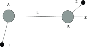
Figure 2: Two ions placed on the distance $L$ and centers of their electronic clouds.

Following the Born-Oppenheimer approximation, slowly oscillating ions are assumed fixed. Let the temperature be low enough $(T\rightarrow 0)$, so only zero-point fluctuations of electrons would be taken into consideration.

In this case, the Hamiltonian of the system can be written as:

$$H=H_{0}+H^{\prime}$$

$$H_{0}=-\frac{\hbar^{2}}{4m_{e}}\left(\nabla_{1}^{2}+\nabla_{2}^{2}\right)-\frac{4e^{2}}{r_{1}}-\frac{4e^{2}}{r_{2}}$$ (2)

$$H^{\prime}=\frac{4e^{2}}{L}+\frac{4e^{2}}{r_{12}}-\frac{4e^{2}}{r_{1B}}-\frac{4e^{2}}{r_{2A}}$$

Eigenfunctions of the unperturbed Hamiltonian describes two ions surrounded by electronic clouds without interactions between them. Due to the fact that the distance between the ions is large compared with the size of the electron clouds $L\gg r$ , the additional term $H^{\prime}$ characterizing the interaction can be regarded as a perturbation.

If we are interested in the leading term of the interaction energy for L, the function $H^{\prime}$ can be expanded in a series in powers of $1/L$ and we can write the first term:

$$\begin{array}[]{l}{H^{\prime}=\frac{4e^{2}}{L}\biggl{\{}1+}\\ +\left[1+\frac{2(z_{2}-z_{1})}{L}+\frac{(x_{2}-x_{1})^{2}+(y_{2}-y_{1})^{2}+(z_{2}-z_{1})^{2}}{L^{2}}\right]^{-1/2}-\\ \left.-\left(1-\frac{2z_{1}}{L}+\frac{r_{1}^{2}}{L^{2}}\right)^{-1/2}-\left(1+\frac{2z_{2}}{L}+\frac{r_{2}^{2}}{L^{2}}\right)^{-1/2}\right\}.\end{array}$$ (3)

After combining the terms in this expression, we get:

$$H^{\prime}\approx\frac{4e^{2}}{L^{3}}\left(x_{1}x_{2}+y_{1}y_{2}-2z_{1}z_{2}\right).$$ (4)

This expression describes the interaction of two dipoles $d_{1}$ and $d_{2}$, which are formed by fixed ions and electronic clouds of the corresponding instantaneous configuration.

Let us determine the displacements of electrons which lead to an attraction in the system .

Let zero-point fluctuations of the dipole moments formed by ions with their electronic clouds occur with the frequency $\Omega_{0}$, whereas each dipole moment can be decomposed into three orthogonal projection $d_{x}=ex,d_{y}=ey$ and $d_{z}=ez$, and fluctuations of the second clouds are shifted in phase on $\varphi_{x},\varphi_{y}$ and $\varphi_{z}$ relative to fluctuations of the first.

As can be seen from Eq.(4), the interaction of z-components is advantageous at in-phase zero-point oscillations of clouds, i.e., when $\varphi_{z}=2\pi$.

Since the interaction of oscillating electric dipoles is due to the occurrence of oscillating electric field generated by them, the phase shift on $2\pi$ means that attracting dipoles are placed along the z-axis on the wavelength $\Lambda_{0}$:

$$L_{z}=\Lambda_{0}=\frac{c}{2\pi\Omega_{0}}.$$ (5)

As follows from (4), the attraction of dipoles at the interaction of the x and y-component will occur if these oscillations are antiphase, i.e. if the dipoles are separated along these axes on the distance equals to half of the wavelength:

$$L_{x,y}=\frac{\Lambda_{0}}{2}=\frac{c}{4\pi\Omega_{0}}.$$ (6)

In this case

$$H^{\prime}=-{4e^{2}}\left(\frac{x_{1}x_{2}}{L_{x}^{3}}+\frac{y_{1}y_{2}}{L_{y}^{3}}+2\frac{z_{1}z_{2}}{L_{z}^{3}}\right).$$ (7)

Assuming that the electronic clouds have isotropic oscillations with amplitude $a_{0}$ for each axis

$$x_{1}=x_{2}=y_{1}=y_{2}=z_{1}=z_{2}=a_{0}$$ (8)

we obtain

$$H^{\prime}=576\pi^{3}\frac{e^{2}}{c^{3}}\Omega_{0}^{3}a_{0}^{2}.$$ (9)

1.1.4 The zero-point oscillations amplitude

The principal condition for the superconducting state formation, that is the ordering of zero-point oscillations, is realized due to the fact that the paired electrons, which obey Bose-Einstein statistics, interact with each other.

At they interact, their amplitudes, frequencies and phases of zero-point oscillations become ordered.

Let an electron gas has density $n_{e}$ and its Fermi-energy be $\mathcal{E}_{F}$. Each electron of this gas can be considered as fixed inside a cell with linear dimension $\lambda_{F}$:

$$\lambda_{F}^{3}=\frac{1}{n_{e}}$$ (10)

which corresponds to the de Broglie wavelength:

$$\lambda_{F}=\frac{2\pi\hbar}{p_{F}}.$$ (11)

Having taken into account (11), the Fermi energy of the electron gas can be written as

$$\mathcal{E}_{F}=\frac{p_{F}^{2}}{2m_{e}}=2\pi^{2}\frac{e^{2}a_{B}}{\lambda_{F}^{2}}.$$ (12)

However, a free electron interacts with the ion at its zero-point oscillations. If we consider the ions system as a positive background uniformly spread over the cells, the electron inside one cell has the potential energy:

$$\mathcal{E}_{p}\simeq-\frac{e^{2}}{\lambda_{F}}.$$ (13)

As zero-point oscillations of the electron pair are quantized by definition, their frequency and amplitude are related

$${m_{e}a_{0}^{2}\Omega_{0}}\simeq\frac{\hbar}{2}.$$ (14)

Therefore, the kinetic energy of electron undergoing zero-point oscillations in a limited region of space, can be written as:

$$\mathcal{E}_{k}\simeq\frac{\hbar^{2}}{2m_{e}a_{0}^{2}}.$$ (15)

In accordance with the virial theorem [10], if a particle executes a finite motion, its potential energy $\mathcal{E}_{p}$ should be associated with its kinetic energy $\mathcal{E}_{k}$ through the simple relation $|\mathcal{E}_{p}|=2\mathcal{E}_{k}$.

In this regard, we find that the amplitude of the zero-point oscillations of an electron in a cell is:

$$a_{0}\simeq\sqrt{2\lambda_{F}a_{B}}.$$ (16)

1.1.5 The condensation temperature

Hence the interaction energy, which unites particles into the condensate of ordered zero-point oscillations

$$\Delta_{0}\equiv H^{\prime}=18\pi^{3}\alpha^{3}\frac{e^{2}a_{B}}{\lambda_{F}^{2}},$$ (17)

where $\alpha=\frac{1}{137}$ is the fine structure constant.

Comparing this association energy with the Fermi energy (12), we obtain

$$\frac{\Delta_{0}}{\mathcal{E}_{F}}=9\pi\alpha^{3}\simeq 1.1\cdot 10^{-5}.$$ (18)

Assuming that the critical temperature below which the possible existence of such condensate is approximately equal

$$T_{c}\simeq\frac{1}{2}\frac{\Delta_{0}}{k}$$ (19)

(the coefficient approximately equal to 1/2 corresponds to the experimental data, discussed below in the subsection (1.2.6)).

After substituting obtained parameters, we have

$$T_{c}\simeq 5.5\cdot 10^{-6}{T}_{F}$$ (20)

The experimentally measured ratios $\frac{T_{c}}{T_{F}}$ for I-type superconductors are given in Table (1) and in Fig.(3).

The straight line on this figure is obtained from Eq.(20), which as seen defines an upper limit of critical temperatures of I-type superconductors.

1.2 The condensate of zero-point oscillations and type-I superconductors

1.2.1 The critical temperature of type-I superconductors

In order to compare the critical temperature of the condensate of zero-point oscillations with measured critical temperatures of superconductors, at first we should make an estimation on the Fermi energies of superconductors. For this we use the experimental data for the Sommerfeld‘s constant through which the Fermi energy can be expressed:

$$\gamma=\frac{\pi^{2}k^{2}n_{e}}{4\mathcal{E}_{F}}=\frac{1}{2}\cdot\left(\frac{\pi}{3}\right)^{2/3}\left(\frac{k}{\hbar}\right)^{2}m_{e}n_{e}^{1/3}$$ (21)

So on the basis of Eqs.(12) and (21), we get:

$$kT_{F}(\gamma)=\frac{p_{F}^{2}(\gamma)}{2m_{e}}\simeq\left(\frac{12}{k^{2}}\right)^{2}\left(\frac{\hbar^{2}}{2m_{e}}\right)^{3}\gamma^{2}.$$ (22)

On base of these calculations we obtain possibility to relate directly the critical temperature of a superconductor with the experimentally measurable parameter: with its electronic specific heat.

Taking into account Eq.(20), we have:

$$\Delta_{0}\simeq\Theta\gamma^{2},$$ (23)

where the constant

$$\Theta\simeq 31\frac{\pi^{2}}{k}\left[\frac{\alpha\hbar^{2}}{km_{e}}\right]^{3}\simeq 6.65\cdot 10^{-22}\frac{K^{4}cm^{6}}{erg}.$$ (24)

The comparison of the calculated parameters and measured data ([11],[12]) is given in Table (1)-(2) and in Fig.(3) and (8).

superconductor	$T_{c}$,K	$T_{F}$,K	$\frac{T_{c}}{T_{F}}$
		Eq(22)
Cd	0.51	$1.81\cdot 10^{5}$	$2.86\cdot 10^{-6}$
Zn	0.85	$3.30\cdot 10^{5}$	$2.58\cdot 10^{-6}$
Ga	1.09	$1.65\cdot 10^{5}$	$6.65\cdot 10^{-6}$
Tl	2.39	$4.67\cdot 10^{5}$	$5.09\cdot 10^{-6}$
In	3.41	$7.22\cdot 10^{5}$	$4.72\cdot 10^{-6}$
Sn	3.72	$7.33\cdot 10^{5}$	$5.08\cdot 10^{-6}$
Hg	4.15	$1.05\cdot 10^{6}$	$3.96\cdot 10^{-6}$
Pb	7.19	$1.85\cdot 10^{6}$	$3.90\cdot 10^{-6}$

Table 1: The comparison of the calculated values of superconductors critical temperatures with measured Fermi temperatures

Figure 3: The comparison of critical temperatures $T_{c}$ of type-I superconductors with their Fermi temperatures $T_{F}$. The straight line is obtained from Eq.(20).

super-	$T_{c}$(measur),	$\gamma,\frac{erg}{cm^{3}K^{2}}$	$T_{c}$(calc),K	$\frac{T_{c}(calc)}{T_{c}(meas)}$
conductors	K		Eq.(23)
Cd	$0.517$	532	$0.77$	1.49
Zn	$0.85$	718	$1.41$	1.65
Ga	$1.09$	508	$0.70$	0.65
Tl	$2.39$	855	$1.99$	0.84
In	$3.41$	1062	$3.08$	0.90
Sn	$3.72$	1070	$3.12$	0.84
Hg	$4.15$	1280	$4.48$	1.07
Pb	$7.19$	1699	$7.88$	1.09

Table 2: The comparison of the calculated values of superconductors critical temperatures with measurement data

1.2.2 The relation of critical parameters of type-I superconductors

The phenomenon of condensation of zero-point oscillations in the electron gas has its characteristic features.

There are several ways of destroying the zero-point oscillations condensate in electron gas:

Firstly, it can be evaporated by heating. In this case, evaporation of the condensate should possess the properties of an order-disorder transition.

Secondly, due to the fact that the oscillating electrons carry electric charge, the condensate can be destroyed by the application of a sufficiently strong magnetic field.

For this reason, the critical temperature and critical magnetic field of the condensate will be interconnected.

This interconnection should manifest itself through the relationship of the critical temperature and critical field of the superconductors, if superconductivity occurs as result of an ordering of zero-point fluctuations.

Let us assume that at a given temperature ${T<T_{c}}$ the system of vibrational levels of conducting electrons consists of only two levels:

firstly, basic level which is characterized by an anti-phase oscillations of the electron pairs at the distance $\Lambda_{0}/2$, and

secondly, an excited level characterized by in-phase oscillation of the pairs.

Let the population of the basic level be $N_{0}$ particles and the excited level has $N_{1}$ particles.

Two electron pairs at an in-phase oscillations have a high energy of interaction and therefore cannot form the condensate. The condensate can be formed only by the particles that make up the difference between the populations of levels $N_{0}-N_{1}$. In a dimensionless form, this difference defines the order parameter:

$$\Psi=\frac{N_{0}}{N_{0}+N_{1}}-\frac{N_{1}}{N_{0}+N_{1}}.$$ (25)

In the theory of superconductivity, by definition, the order parameter is determined by the value of the energy gap

$$\Psi=\Delta_{T}/\Delta_{0}.$$ (26)

When taking a counting of energy from the level $\varepsilon_{0}$, we obtain

$$\frac{\Delta_{T}}{\Delta_{0}}=\frac{N_{0}-N_{1}}{N_{0}+N_{1}}\simeq\frac{e^{2\Delta_{T}/kT}-1}{e^{2\Delta_{T}/kT}+1}=th(2\Delta_{T}/kT).$$ (27)

Passing to dimensionless variables $\delta\equiv\frac{\Delta_{T}}{\Delta_{0}}$ , $t\equiv\frac{kT}{kT_{c}}$ and $\beta\equiv\frac{2\Delta_{0}}{kT_{c}}$ we have

$$\delta=\frac{e^{\beta\delta/t}-1}{e^{\beta\delta/t}+1}=th(\beta\delta/t).$$ (28)

This equation describes the temperature dependence of the energy gap in the spectrum of zero-point oscillations. It is similar to other equations describing other physical phenomena, that are also characterized by the existence of the temperature dependence of order parameters [13],[14]. For example, this dependence is similar to temperature dependencies of the concentration of the superfluid component in liquid helium or the spontaneous magnetization of ferromagnetic materials. This equation is the same for all order-disorder transitions (the phase transitions of 2nd-type in the Landau classification).

The solution of this equation, obtained by the iteration method, is shown in Fig.(4).

Figure 4: The temperature dependence of the value of the gap in the energetic spectrum of zero-point oscillations calculated on Eq.(28).

This decision is in a agreement with the known transcendental equation of the BCS, which was obtained by the integration of the phonon spectrum, and is in a satisfactory agreement with the measurement data.

After numerical integrating we can obtain the averaging value of the gap:

$$\langle\Delta\rangle=\Delta_{0}\int_{0}^{1}\delta dt=0.852~{}\Delta_{0}~{}.$$ (29)

To convert the condensate into the normal state, we must raise half of its particles into the excited state (according to Eq.(27), the gap collapses under this condition). To do this, taking into account Eq.(29), the unit volume of condensate should have the energy:

$$\mathcal{E}_{T}\simeq\frac{1}{2}n_{0}\langle\Delta_{0}\rangle\approx\frac{0.85}{2}\left(\frac{m_{e}}{2\pi^{2}\alpha\hbar^{2}}\right)^{3/2}\Delta_{0}^{5/2},$$ (30)

On the other hand, we can obtain the normal state of an electrically charged condensate when applying a magnetic field of critical value $H_{c}$ with the density of energy:

$$\mathcal{E}_{H}=\frac{H_{c}^{2}}{8\pi}.$$ (31)

As a result, we acquire the condition:

$$\frac{1}{2}n_{0}\langle\Delta_{0}\rangle=\frac{H_{c}^{2}}{8\pi}.$$ (32)

This creates a relation of the critical temperature to the critical magnetic field of the zero-point oscillations condensate of the charged bosons.

The comparison of the critical energy densities $\mathcal{E}_{T}$ and $\mathcal{E}_{H}$ for type-I superconductors are shown in Fig.(5).

Figure 5: The comparison of the critical energy densities $\mathcal{E}_{T}$ (Eq.(30)) and $\mathcal{E}_{H}$ (Eq.(31)) for the type-I superconductors.

As shown, the obtained agreement between the energies $\mathcal{E_{T}}$ (Eq.(30)) and $\mathcal{E_{H}}$ (Eq.(31)) is quite satisfactory for type-I superconductors [11],[12]. A similar comparison for type-II superconductors shows results that differ by a factor two approximately. The reason for this will be considered below. The correction of this calculation, has not apparently made sense here. The purpose of these calculations was to show that the description of superconductivity as the effect of the condensation of ordered zero-point oscillations is in accordance with the available experimental data. This goal is considered reached in the simple case of type-I superconductors.

1.2.3 The critical magnetic field of superconductors

The direct influence of the external magnetic field of the critical value applied to the electron system is too weak to disrupt the dipole-dipole interaction of two paired electrons:

$$\mu_{B}H_{c}\ll kT_{c}.$$ (33)

In order to violate the superconductivity so as to destroy the ordering of the electron zero-point oscillations. For this the presence of relatively weak magnetic field is required.

At combing of Eqs.(32),(30) and (16), we can express the gap through the critical magnetic field and the magnitude of the oscillating dipole moment:

$$\Delta_{0}\approx\frac{1}{2}~{}e~{}a_{0}~{}H_{c}.$$ (34)

The properties of the zero-point oscillations of the electrons should not be dependent on the characteristics of the mechanism of association and also on the condition of the existence of electron pairs. Therefore, we should expect that this equation would also be valid for type-I superconductors, as well as for II-type superconductors (for II-type superconductor $H_{c}=H_{c1}$ is the first critical field)

An agreement with this condition is illustrated on the Fig.(6).

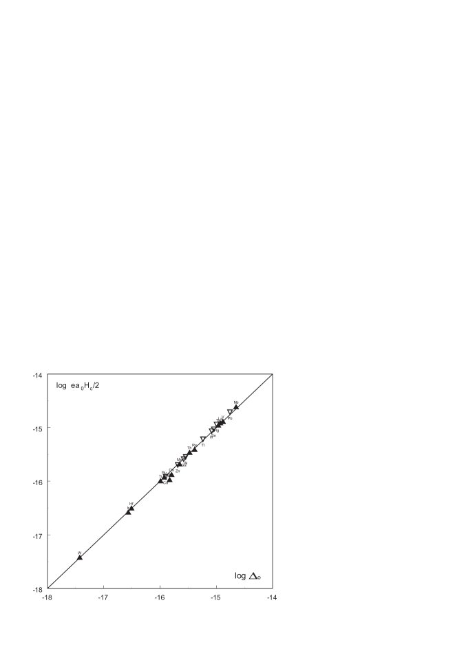
Figure 6: The comparison of the calculated energy of superconducting pairs in the critical magnetic field with the value of the superconducting gap. Here, the following key applies: filled triangles - type-II superconductors, empty triangles - type-I superconductors. On vertical axis - logarithm of the product of the calculated value of the oscillating dipole moment of an electron pair on the critical magnetic field is plotted.On horizontal axis - the value of the gap is shown.

1.2.4 The density of superconducting carriers

Let us consider the process of heating the electron gas in metal. When heating, the electrons from levels slightly below the Fermi-energy are raised to higher levels. As a result, the levels closest to the Fermi level, from which at low temperature electrons were forming bosons, become vacant.

At critical temperature $T_{c}$, all electrons from the levels of energy bands from $\mathcal{E}_{F}-\Delta$ to $\mathcal{E}_{F}$ move to higher levels (and the gap collapses). At this temperature superconductivity is therefore destroyed completely.

This band of energy can be filled by $N_{\Delta}$ particles:

$$N_{\Delta}=2\int_{\mathcal{E}_{F}-\Delta}^{\mathcal{E}_{F}}F(\mathcal{E})D(\mathcal{E})d\mathcal{E}.$$ (35)

Where $F(\mathcal{E})=\frac{1}{e^{\frac{\mathcal{E}-\mu}{\tau}}+1}$ is the Fermi-Dirac function and $D(\mathcal{E})$ is number of states per an unit energy interval, a deuce front of the integral arises from the fact that there are two electron at each energy level.

To find the density of states $D(\mathcal{E})$, one needs to find the difference in energy of the system at $T=0$ and finite temperature:

$$\Delta\mathcal{E}=\int_{0}^{\infty}F(\mathcal{E})\mathcal{E}D(\mathcal{E})d\mathcal{E}-\int_{0}^{\mathcal{E}_{F}}\mathcal{E}D(\mathcal{E})d\mathcal{E}.$$ (36)

For the calculation of the density of states $D(\mathcal{E})$, we must note that two electrons can be placed on each level. Thus, from the expression of the Fermi-energy Eq.(12) we obtain

$$D({E}_{F})=\frac{1}{2}\cdot\frac{dn_{e}}{d\mathcal{E}_{F}}=\frac{3n_{e}}{4\mathcal{E}_{F}}=\frac{3\gamma}{2k^{2}\pi^{2}},$$ (37)

where

$$\gamma=\frac{\pi^{2}k^{2}n_{e}}{4\mathcal{E}_{F}}=\frac{1}{2}\cdot\left(\frac{\pi}{3}\right)^{3/2}\left(\frac{k}{\hbar}\right)^{2}m_{e}n_{e}^{1/3}$$ (38)

is the Sommerfeld constant .

Using similar arguments, we can calculate the number of electrons, which populate the levels in the range from $\mathcal{E}_{F}-\Delta$ to $\mathcal{E}_{F}$. For an unit volume of material, Eq.(35) can be rewritten as:

$$n_{\Delta}=2kT\cdot D(\mathcal{E}_{F})\int_{-\frac{\Delta_{0}}{kT_{c}}}^{0}\frac{dx}{(e^{x}+1)}.$$ (39)

By supposing that for superconductors $\frac{\Delta_{0}}{kT_{c}}=1.76$, as a result of numerical integration we obtain

$$\int_{-\frac{\Delta_{0}}{kT_{c}}}^{0}\frac{dx}{(e^{x}+1)}=\left[x-ln(e^{x}+1)\right]_{-1.76}^{0}\approx 1.22.$$ (40)

Thus, the density of electrons, which throw up above the Fermi level in a metal at temperature $T=T_{c}$ is

$$n_{e}(T_{c})\approx 2.44\left(\frac{3\gamma}{k^{2}\pi^{2}}\right)kT_{c}.$$ (41)

Where the Sommerfeld constant $\gamma$ is related to the volume unit of the metal.

From Eq.(6) it follows

$$L_{0}\simeq\frac{\lambda_{F}}{\pi\alpha}$$ (42)

and this forms the ratio of the condensate particle density to the Fermi gas density:

$$\frac{n_{0}}{n_{e}}=\frac{\lambda_{F}^{3}}{L_{0}^{3}}\simeq\left(\pi\alpha\right)^{3}\simeq 10^{-5}.$$ (43)

When using these equations, we can find a linear dimension of localization for an electron pair:

$$L_{0}=\frac{\Lambda_{0}}{2}\simeq\frac{1}{\pi\alpha(n_{e})^{1/3}}.$$ (44)

or, taking into account Eq.(16), we can obtain the relation between the density of particles in the condensate and the value of the energy gap:

$$\Delta_{0}\simeq 2\pi^{2}\alpha\frac{\hbar^{2}}{m_{e}}n_{0}^{2/3}$$ (45)

or

$$n_{0}=\frac{1}{L_{0}^{3}}=\left(\frac{m_{e}}{2\pi^{2}\alpha\hbar^{2}}\Delta_{0}\right)^{3/2}.$$ (46)

It should be noted that the obtained ratios for the zero-point oscillations condensate (of bose-particles) differ from the corresponding expressions for the bose-condensate of particles, which can be obtained in many courses (see eg [13]). The expressions for the ordered condensate of zero-point oscillations have an additional coefficient $\alpha$ on the right side of Eq.(45).

The de Broglie wavelengths of Fermi electrons expressed through the Sommerfelds constant

$$\lambda_{F}=\frac{2\pi\hbar}{p_{F}(\gamma)}\simeq\frac{\pi}{3}\cdot\frac{k^{2}m_{e}}{\hbar^{2}\gamma}$$ (47)

are shown in Tab.3.

In accordance with Eq.(42), which was obtained at the zero-point oscillations consideration, the ratio $\frac{\lambda_{F}}{\Lambda_{0}}\simeq 2.3\cdot 10^{-2}$.

In connection with this ratio, the calculated ratio of the zero-point oscillations condensate density to the density of fermions in accordance with Eq.(43) should be near to $10^{-5}$.

It can be therefore be seen, that calculated estimations of the condensate parameters are in satisfactory agreement with experimental data of superconductors.

super-	$\lambda_{F}$,cm	$\Lambda_{0}$,cm	$\frac{\lambda_{F}}{\Lambda_{0}}$	$\frac{n_{0}}{n_{e}}=\left(\frac{\lambda_{F}}{\Lambda_{0}}\right)^{3}$
conductor	Eq(47)	Eq(6)
Cd	$3.1\cdot 10^{-8}$	$1.18\cdot 10^{-6}$	$2.6\cdot 10^{-2}$	$1.8\cdot 10^{-5}$
Zn	$2.3\cdot 10^{-8}$	$0.92\cdot 10^{-6}$	$2.5\cdot 10^{-2}$	$1.5\cdot 10^{-5}$
Ga	$3.2\cdot 10^{-8}$	$0.81\cdot 10^{-6}$	$3.9\cdot 10^{-2}$	$6.3\cdot 10^{-5}$
Tl	$1.9\cdot 10^{-8}$	$0.55\cdot 10^{-6}$	$3.4\cdot 10^{-2}$	$4.3\cdot 10^{-5}$
In	$1.5\cdot 10^{-8}$	$0.46\cdot 10^{-6}$	$3.2\cdot 10^{-2}$	$3.8\cdot 10^{-5}$
Sn	$1.5\cdot 10^{-8}$	$0.44\cdot 10^{-6}$	$3.4\cdot 10^{-2}$	$4.3\cdot 10^{-5}$
Hg	$1.3\cdot 10^{-8}$	$0.42\cdot 10^{-6}$	$3.1\cdot 10^{-2}$	$2.9\cdot 10^{-5}$
Pb	$1.0\cdot 10^{-8}$	$0.32\cdot 10^{-6}$	$3.1\cdot 10^{-2}$	$2.9\cdot 10^{-5}$

Table 3: The ratios $\frac{\lambda_{F}}{\Lambda_{0}}$ and $\frac{n_{0}}{n_{e}}$ for type-I superconductors

Based on these calculations, it is interesting to compare the density of superconducting carriers $n_{0}$ at $T=0$, which is described by Eq.(46), with the density of normal carriers $n_{e}(T_{c})$, which are evaporated on levels above $\mathcal{E}_{F}$ at $T=T_{c}$ and are described by Eq.(41).

Figure 7: The comparison of the number of superconducting carriers at $T=0$ with the number of thermally activated electrons at $T=T_{c}$.

This comparison is shown in Table (4) and Fig.7. (Data has been taken from the tables [11],[12]).

superconductor	$n_{0}$	$n_{e}({T_{c}})$	$2n_{0}/n_{e}(T_{c})$
Cd	$6.11\cdot 10^{17}$	$1.48\cdot 10^{18}$	0.83
Zn	$1.29\cdot 10^{18}$	$3.28\cdot 10^{18}$	0.78
Ga	$1.85\cdot 10^{18}$	$2.96\cdot 10^{18}$	1.25
Al	$2.09\cdot 10^{18}$	$8.53\cdot 10^{18}$	0.49
Tl	$6.03\cdot 10^{18}$	$1.09\cdot 10^{19}$	1.10
In	$1.03\cdot 10^{19}$	$1.94\cdot 10^{19}$	1.06
Sn	$1.18\cdot 10^{19}$	$2.14\cdot 10^{19}$	1.10
Hg	$1.39\cdot 10^{19}$	$2.86\cdot 10^{19}$	0.97
Pb	$3.17\cdot 10^{19}$	$6.58\cdot 10^{19}$	0.96

Table 4: The comparison of the superconducting carriers density at $T=0$ with the density of thermally activated electrons at $T=T_{c}$

From the data described above, we can obtain the condition of destruction of superconductivity, after heating for superconductors of type-I, as written in the equation:

$${n_{e}}{({T_{c}})}\simeq 2{n_{0}}$$ (48)

1.2.5 The sound velocity of the zero-point oscillations condensate

The wavelength of zero-point oscillations $\Lambda_{0}$ in this model is an analogue of the Pippard coherence length in the BCS. As usually accepted [11], the coherence length $\xi=\frac{\hbar v_{F}}{4\Delta_{0}}$. The ratio of these lengths, taking into account Eq.(20), is simply the constant:

$$\frac{\Lambda_{0}}{\xi}\approx 8\pi^{2}\alpha^{2}\approx\cdot 10^{-3}.$$ (49)

The attractive forces arising between the dipoles located at a distance $\frac{\Lambda_{0}}{2}$ from each other and vibrating in opposite phase, create pressure in the system:

$$P\simeq\frac{d\Delta_{0}}{dV}\simeq\frac{d_{\Omega}^{2}}{L_{0}^{6}}.$$ (50)

In this regard, sound into this condensation should propagate with the velocity:

$$c_{s}\simeq\sqrt{\frac{1}{2m_{e}}\frac{dP}{dn_{0}}}.$$ (51)

After the appropriate substitutions, the speed of sound in the condensate can be expressed through the Fermi velocity of electron gas

$$c_{s}\simeq\sqrt{2\pi^{2}\alpha^{3}}v_{F}\simeq 10^{-2}v_{F}.$$ (52)

The condensate particles moving with velocity $c_{S}$ have the kinetic energy:

$${2m_{e}c_{s}^{2}}\simeq\Delta_{0}.$$ (53)

Therefore, by either heating the condensate to the critical temperature when each of its volume obtains the energy $\mathcal{E}\approx n_{0}\Delta_{0}$, or initiating the current of its particles with a velocity exceeding $c_{S}$, can achieve the destruction of the condensate. (Because the condensate of charged particles oscillations is considered, destroying its coherence can be also obtained at the application of a sufficiently strong magnetic field. See below.)

1.2.6 The relationship $\Delta_{0}/kT_{c}$

From Eq.(48) and taking into account Eqs.(23),(41) and (46), which were obtained for condensate, we have:

$$\frac{\Delta_{0}}{kT_{c}}\simeq 1.86.$$ (54)

This estimation of the relationship $\Delta_{0}/kT_{c}$ obtained for condensate has a satisfactory agreement with the measured data [12], for type-I superconductors as listed in Table (5).

superconductor	$T_{c}$,K	$\Delta_{0}$,mev	$\frac{\Delta_{0}}{kT_{c}}$
Cd	0.51	0.072	1.64
Zn	0.85	0.13	1.77
Ga	1.09	0.169	1.80
Tl	2.39	0.369	1.79
In	3.41	0.541	1.84
Sn	3.72	0.593	1.85
Hg	4.15	0.824	2.29
Pb	7.19	1.38	2.22

Table 5: The value of ratio $\Delta_{0}/kT_{c}$ obtained experimentally for type-I superconductors

1.3 Another superconductors

1.3.1 About type-II superconductors

The estimation of properties of type-II superconductors

In the case of type-II superconductors the situation is more complicated.

In this case, measurements show that these metals have an electronic specific heat that has an order of value greater than those calculated on the base of free electron gas model.

The peculiarity of these metals is associated with the specific structure of their ions. They are transition metals with unfilled inner d-shell (see Table 6).

It can be assumed that the increase in the electronic specific heat of these metals should be associated with a characteristic interaction of free electrons with the electrons of the unfilled d-shell.

superconductors	electron shells
$Ti$	$3d^{2}~{}4s^{2}$
$V$	$3d^{3}~{}4s^{2}$
$Zr$	$4d^{2}~{}5s^{2}$
$Nb$	$4d^{3}~{}5s^{2}$
$Mo$	$4d^{4}~{}5s^{2}$
$Tc$	$4d^{5}~{}5s^{2}$
$Ru$	$4d^{6}~{}5s^{2}$
$La$	$5d^{1}~{}6s^{2}$
$Hf$	$5d^{2}~{}6s^{2}$
$Ta$	$5d^{3}~{}6s^{2}$
$W$	$5d^{4}~{}6s^{2}$
$Re$	$5d^{5}~{}6s^{2}$
$Os$	$5d^{6}~{}6s^{2}$
$Ir$	$5d^{7}~{}6s^{2}$

Table 6: The external electron shells of elementary type-II superconductors

Since the heat capacity of the ionic lattice of metals is negligible at low temperatures, only the electronic subsystem is thermally active .

At $T=0$ the superconducting careers populates the energetic level $\mathcal{E}_{F}-\Delta_{0}$. During the destruction of superconductivity through heating, an each heated career increases its thermal vibration. If the effective velocity of vibration is $v_{t}$, its kinetic energy:

$$\mathcal{E}_{k}=\frac{mv_{t}^{2}}{2}\simeq\Delta_{0}$$ (55)

Only a fraction of the heat energy transferred to the metal is consumed in order to increase the kinetic energy of the electron gas in the transition metals.

Another part of the energy will be spent on the magnetic interaction of a moving electron.

At contact with the d-shell electron, a freely moving electron induces onto it the magnetic field of the order of value:

$$H\approx\frac{e}{r_{c}^{2}}\frac{v}{c}.$$ (56)

The magnetic moment of d-electron is approximately equal to the Bohr magneton. Therefore the energy of the magnetic interaction between a moving electron of conductivity and a d-electron is approximately equal to:

$$\mathcal{E}_{\mu}\approx\frac{e^{2}}{2r_{c}}\frac{v}{c}.$$ (57)

This energy is not connected with the process of destruction of superconductivity.

Whereas, in metals with a filled d-shell (type-I superconductors), the whole heating energy increases the kinetic energy of the conductivity electrons and only a small part of the heating energy is spent on it in transition metals:

$$\frac{\mathcal{E}_{k}}{\mathcal{E}_{\mu}+\mathcal{E}_{k}}\simeq\frac{mv_{t}}{h}a_{B}.$$ (58)

So approximately

$$\frac{\mathcal{E}_{k}}{\mathcal{E}_{\mu}+\mathcal{E}_{k}}\simeq\frac{a_{B}}{L_{0}}.$$ (59)

Therefore, whereas the dependence of the gap in type-I superconductors from the heat capacity is defined by Eq.(23), it is necessary to take into account the relation Eq.(59) in type-II superconductors for the determination of this gap dependence. As a result of this estimation, we can obtain:

$$\Delta_{0}\simeq\Theta\gamma^{2}\left(\frac{\mathcal{E}_{k}}{\mathcal{E}_{\mu}+\mathcal{E}_{k}}\right)\simeq\Theta\gamma^{2}\left(\frac{a_{B}}{L_{0}}\right)\frac{1}{2},$$ (60)

where $1/2$ is the fitting parameter.

The comparison of the results of these calculations with the measurement data (Fig.(8)) shows that for the majority of type-II superconductors the estimation Eq.(60) can be considered quite satisfactory.

Figure 8: The comparison of the calculated values of critical temperatures of superconductors with measurement data. Circles relate to type-I superconductors, squares show type-II superconductors. On the abscissa, the measured values of critical temperatures are plotted, on ordinate, the calculated estimations are plotted. The calculations of critical temperatures for type-I superconductors were made by using Eq.(23) and the estimations for type-II superconductors was obtained by using Eq.(60).

1.3.2 Alloys and high-temperature superconductors

In order to understand the mechanism of high temperature superconductivity, it is important to establish whether the high-$T_{c}$ ceramics are the I or II-type superconductors, or whether they are a special class of superconductors.

In order to determine this, we need to look at the above established dependence of critical parameters from the electronic specific heat and also consider that the specific heat of superconductors I and II-types are differing considerably.

There are some difficulties by determining the answer this way: as we do not precisely know the density of the electron gas in high-temperature superconductors. However, the densities of atoms in metals do not differ too much and we can use Eq.(23) for the solution of the problem of the I- and II-types superconductors distinguishing.

If parameters of type-I superconductors are inserted into this equation, we obtain quite a satisfactory estimation of the critical temperature (as was done above, see Fig.8). For the type-II superconductors‘ values, this assessment gives an overestimated value due to the fact that type-II superconductors’ specific heat has additional term associated with the magnetization of d-electrons.

This analysis therefore, illustrates a possibility where we can divide all superconductors into two groups, as is evident from the Fig.(9).

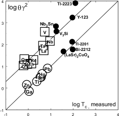
Figure 9: The comparison of the calculated parameter $\Theta\gamma^{2}$ with the measurement of the critical temperatures of elementary superconductors and some superconducting compounds.

It is generally assumed that we consider alloys $Nb_{3}Sn$ and $V_{3}Si$ as the type-II superconductors. This assumption seems quite normal because they are placed in close surroundings of Nb. Some excess of the calculated critical temperature over the experimentally measured value for ceramics $Ta_{2}Ba_{2}Ca_{2}Cu_{3}O_{10}$ can be attributed to the measured heat capacity that may have been created by not only conductive electrons, but also non-superconducting elements (layers) of ceramics. It is already known that it, as well as ceramics $YBa_{2}Cu_{3}O_{7}$, belongs to the type-II superconductors. However, ceramics (LaSr)₂Cu₄, Bi-2212 and Tl-2201, according to this figure should be regarded as type-I superconductors, which is unusual.

1.4 About the London penetration depth

1.4.1 The traditional approach to calculation of the London penetration depth

The consideration of the London penetration depth is commonly accepted (see, for example [11]) in several steps:

Step 1.

Firstly, the action of an external electric field on free electrons is considered. In accordance with Newton’s law, free electrons gain acceleration in an electric field $\mathbf{E}$:

$$\mathbf{a}=\frac{e{\mathbf{E}}}{m_{e}}.$$ (61)

The directional movement of the ”superconducting”  electron gas with the density $n_{s}$ creates the current with the density:

$$\mathbf{j}=en_{s}\mathbf{v},$$ (62)

where $\mathbf{v}$ is the carriers velocity.

After differentiating the time and substituting this in Eq.(61), we obtain the first London’s equation:

$$\frac{d}{dt}\mathbf{j}=en_{s}\mathbf{a}=\frac{n_{s}e^{2}}{m_{e}}\mathbf{E}.$$ (63)

Step 2.

After application of operations $rot$ to both sides of this equation and by using the Faraday’s law of electromagnetic induction $rot\mathbf{E}=-\frac{1}{c}\frac{d\mathbf{B}}{dt}$ we acquire the relationship between the current density and magnetic field:

$$\frac{d}{dt}\left(rot~{}\mathbf{j}+\frac{n_{s}e^{2}}{m_{e}c}\mathbf{B}\right)=0.$$ (64)

Step 3. By selecting the stationary solution of Eq.(64)

$$rot~{}\mathbf{j}+\frac{n_{s}e^{2}}{m_{e}c}\mathbf{B}=0,$$ (65)

and after some simple transformations, we can conclude that there is a so-called London penetration depth of the magnetic field in a superconductor:

$$\Lambda_{L}=\sqrt{\frac{m_{e}c^{2}}{4\pi e^{2}n_{s}}}.$$ (66)

1.4.2 The London penetration depth and the density of superconducting carriers

One of the measurable characteristics of superconductors is the London penetration depth, and for many of these superconductors it usually equals to a few hundred Angstroms [15]. In the Table (1.4.2) the measured values of $\lambda_{L}$ are given in the second column.

	$\lambda_{L}$,$10^{-6}$cm	$n_{s}$	$n_{e}$
super-	measured	according to	in accordance	$n_{s}/n_{e}$
conductors	[15]	Eq.(66)	with Eq.(47)
Tl	9.2	$3.3\cdot 10^{21}$	$1.4\cdot 10^{23}$	0.023
In	6.4	$6.9\cdot 10^{21}$	$3.0\cdot 10^{23}$	0.024
Sn	5.1	$1.1\cdot 10^{22}$	$3.0\cdot 10^{23}$	0.037
Hg	4.2	$1.6\cdot 10^{22}$	$4.5\cdot 10^{22}$	0.035
Pb	3.9	$1.9\cdot 10^{22}$	$1.0\cdot 10^{24}$	0.019

Table(1.4.2)

If we are to use this experimental data to calculate the density of superconducting carriers $n_{s}$ in accordance with the Eq.(66), the results be about two orders of magnitude larger (see the middle column of Tab.(1.4.2).

Only a small fraction of these free electrons can combine into the pairs. This is only applicable to the electrons that energies lie with in the thin strip of the energy spectrum near $\mathcal{E}_{F}$. We can therefore expect that the concentration of superconducting carriers among all free electrons of the metal should be at the level $\frac{n_{s}}{n_{e}}\approx 10^{-5}$ (see Eq.(43)). These concentrations, if calculated from Eq.(66), are seen to be about two orders of magnitude higher (see last column of the Table (1.4.2).

Apparently, the reason for this discrepancy is because of the use of a nonequivalent transformation. At the first stage in Eq.(61), the straight-line acceleration in a static electric field is considered. If this moves, there will be no current circulation. Therefore, the application of the operation rot in Eq.(64) in this case is not correct. It does not lead to the Eq.(65):

$$\frac{rot~{}\mathbf{j}}{\frac{n_{s}e^{2}}{m_{e}c}\mathbf{B}}=-1,$$ (67)

but instead, leads to a pair of equations:

$$\begin{array}[]{l}rot~{}\mathbf{j}=0\\ \frac{n_{s}e^{2}}{m_{e}c}\mathbf{B}=0\end{array}$$ (68)

and to the uncertainty:

$$\frac{rot~{}\mathbf{j}}{\frac{n_{s}e^{2}}{m_{e}c}\mathbf{B}}=\frac{0}{0}.$$ (69)

1.4.3 The magnetic energy of a moving electron

To avoid these incorrect results, let us consider a balance of magnetic energy in a superconductor within magnetic field. This magnetic energy is composed of energy from a penetrating external magnetic field and magnetic energy of moving electrons.

By using formulas [16], let us estimate the ratio of the magnetic and kinetic energy of an electron (the charge of $e$ and the mass $m_{e}$) when it moves rectilinearly with a velocity $v\ll c$.

The density of the electromagnetic field momentum is expressed by the equation:

$$\mathbf{g}=\frac{1}{4\pi c}[\mathbf{E}\mathbf{H}]$$ (70)

While moving with a velocity $\mathbf{v}$, the electric charge carrying the electric field with intensity $E$ creates a magnetic field

$$\mathbf{H}=\frac{1}{c}[\mathbf{E}\mathbf{v}]$$ (71)

with the density of the electromagnetic field momentum (at $v\ll c$)

$$\mathbf{g}=\frac{1}{4\pi c^{2}}[\mathbf{E}[\mathbf{v}\mathbf{E}]]=\frac{1}{4\pi c^{2}}\left(\mathbf{v}E^{2}-\mathbf{E}(\mathbf{v}\cdot\mathbf{E})\right)$$ (72)

As a result, the momentum of the electromagnetic field of a moving electron

$$\mathbf{G}=\int_{V}\mathbf{g}dV=\frac{1}{4\pi c^{2}}\left(\mathbf{v}\int_{V}E^{2}~{}dV-\int_{V}\mathbf{E}~{}E~{}v~{}cos\vartheta~{}dV\right)$$ (73)

The integrals are taken over the entire space, which is occupied by particle fields, and $\vartheta$ is the angle between the particle velocity and the radius vector of the observation point. By calculating the last integral in the condition of the axial symmetry with respect to $\mathbf{v}$, the contributions from the components of the vector $\mathbf{E}$, which is perpendicular to the velocity, cancel each other for all pairs of elements of the space (if they located diametrically opposite on the magnetic force line). Therefore, according to Eq.(73), the component of the field which is collinear to $\mathbf{v}$

$$\frac{E~{}cos\vartheta\cdot\mathbf{v}}{v}$$ (74)

can be taken instead of the vector $\mathbf{E}$. By taking this information into account, going over to the spherical coordinates and integrating over angles, we can obtain

$$\mathbf{G}=\frac{\mathbf{v}}{4\pi c^{2}}\int_{r}^{\infty}E^{2}\cdot 4\pi r^{2}~{}dr$$ (75)

If we limit the integration of the field by the Compton electron radius $r_{C}=\frac{\hbar}{m_{e}c}$,   then $v\ll c$, and we obtain:

$$\mathbf{G}=\frac{\mathbf{v}}{4\pi c^{2}}\int_{r_{C}}^{\infty}E^{2}\cdot 4\pi r^{2}~{}dr=\frac{\mathbf{v}}{c^{2}}\frac{e^{2}}{r_{C}}.$$ (76)

In this case by taking into account Eq.(71), the magnetic energy of a slowly moving electron pair is equal to:

$$\mathcal{E}=\frac{{v}{G}}{2}=\frac{{v^{2}}}{c^{2}}\frac{e^{2}}{2r_{C}}=\alpha\frac{m_{e}v^{2}}{2}.$$ (77)

1.4.4 The magnetic energy and the London penetration depth

The energy of external magnetic field into volume $dv$:

$$\mathcal{E}=\frac{H^{2}}{8\pi}dv.$$ (78)

At density of superconducting carriers $n_{s}$, their magnetic energy per unit volume in accordance with (77):

$$\mathcal{E}_{H}\simeq\alpha n_{s}\frac{m_{2}v^{2}}{2}=\alpha\frac{m_{e}j_{s}^{2}}{2n_{s}e},$$ (79)

where $j_{s}=2en_{s}v_{s}$ is the density of a current of superconducting carriers.

Taking into account the Maxwell equation

$$\mathbf{rotH}=\frac{4\pi}{c}\mathbf{j}_{s},$$ (80)

the magnetic energy of moving carriers can be written as

$$\mathcal{E}_{H}\simeq\frac{\widetilde{\Lambda}^{2}}{8\pi}(rotH)^{2},$$ (81)

where we introduce the notation

$$\widetilde{\Lambda}=\sqrt{\alpha\frac{m_{e}c^{2}}{4\pi n_{s}e^{2}}}=\sqrt{\alpha}\Lambda_{L}.$$ (82)

In this case, part of the free energy of the superconductor connected with the application of a magnetic field is equal to:

$$\mathcal{F}_{H}=\frac{1}{8\pi}\int_{V}\left(H^{2}+\widetilde{\Lambda}^{2}(rotH)^{2}\right)dv.$$ (83)

At the minimization of the free energy, after some simple transformations we obtain

$$\mathbf{H}+\widetilde{\Lambda}^{2}\mathbf{rotrotH}=0,$$ (84)

thus $\widetilde{\Lambda}$ is the depth of magnetic field penetration into the superconductor.

In view of Eq.(46) from Eq.(82) we can estimate the values of London penetration depth (see table (7)). The consent of the obtained values with the measurement data can be considered quite satisfactory.

super-	$\lambda_{L}$,$10^{-6}$cm	$\widetilde{\Lambda}$,$10^{-6}$cm
conductors	measured [15]	calculated	$\widetilde{\Lambda}/\lambda_{L}$
		Eq.(82)
Tl	9.2	11.0	1.2
In	6.4	8.4	1.3
Sn	5.1	7.9	1.5
Hg	4.2	7.2	1.7
Pb	3.9	4.8	1.2

Table 7: Corrected values of London penetration depth

The resulting refinement can be important for estimations within the frame of Ginzburg-Landau theory, where the London penetration depth is used as a comparison of calculations and specific parameters of superconductors.

1.5 Three words to experimenters

1.5.1 Why creation of room-temperature superconductors is very problematic?

The understanding of the mechanism of the superconducting state should open a way towards finding a solution to the technological problem. This problem was just a dream in the last century: the dream to create a superconductor that would be easily produced (in the sense of ductility) and had high critical temperature.

In order to move towards this goal, it is important firstly to understand the mechanism that limits the critical properties of superconductors.

Let us consider a superconductor with a large limiting current. The length of their localisation determines the limiting momentum of superconducting carriers:

$$p_{c}\simeq\frac{2\pi\hbar}{L_{0}}$$ (85)

Therefore, by using Eq.(53), we can compare the critical velocity of superconducting carriers with the sound velocity:

$$v_{c}=\frac{p_{c}}{2m_{e}}\simeq c_{s}$$ (86)

and these velocities are both about a hundred times smaller than the Fermi velocity.

The sound velocity in the crystal lattice of metal $v_{s}$, in accordance with the Bohm-Staver relation [18], has approximately the same value:

$$v_{s}\simeq\frac{kT_{D}}{E_{F}}v_{F}\simeq 10^{-2}{v_{F}}.$$ (87)

This therefore makes it possible to consider superconductivity being destroyed as a superconducting carrier overcomes the sound barrier. That is, if they moved without friction at a speed that was less than the speed of the sound, after they gained speed and the speed of sound was surpassed, then they acquire a mechanism of friction.

Therefore, it is conceivable that if the speed of sound in the metal lattice $v_{s}<c_{s}$, then it would create a restriction on the limiting current in superconductor.

If this is correct, then superconductors with high critical parameters should have not only a high Fermi energy of their electron gas, but also a high speed of sound in their lattice.

It is in agreement with the fact that ceramics have higher elastic moduli compared to metals and alloys, and also posses much higher critical temperatures (Fig.10).

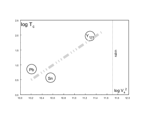
Figure 10: The schematic representation of the dependence of critical temperature on the speed of sound in superconductors. On the ordinate, the logarithm of the superconductor’s critical temperature is shown. On the abscissa, the logarithm of the square of the speed of sound is shown (for Sn and Pb - the transverse velocity of sound is shown, because it is smaller). The speed of sound in a film was used for yttrium-123 ceramics. The dashed line shows the value of the transverse velocity of sound in sapphire, as some estimation of the limit of its value. It can be seen that this estimation leads to the restriction on the critical temperature in the range about $0^{o}$C - the dot-dashed line.

The dependence of the critical temperature on the square of the speed of sound [19] is illustrated in Fig.(10).

This figure, which can be viewed only as a rough estimation due to the lack of necessary experimental data, shows that the elastic modulus of ceramics with a critical temperature close to the room temperature, should be close to the elastic modulus of sapphire, which is very difficult to achieve.

In addition, such ceramics would be deprived from another important quality: their adaptability. Indeed, in order to obtain a thin wire, we require a plastic superconductor.

A solution of this problem would be to find a material that possesses an acceptably high critical temperature (above 80K) and experiences a phase transition at even higher temperature of heat treatment. It would be possible to make a thin wire from a superconductor near the point of phase transition, as the elastic modules are typically not very strong at this stage.

1.5.2 Magnetic electron pairing

The described formation of mechanism for the superconducting state provides a possibility to obtain an estimations of the critical parameters of superconductors, which in most cases is in satisfactory agreement with measured data. For some superconductors, this agreement is stronger, and for other, such as Ir, Al, V (see Fig.(8)), it is expedient to carry out further theoretical and experimental studies due to causes of deviations.

The mechanism of magnetic electron pairing is also very important for further clarification of this phenomenon.

As it was found earlier, in the cylinders made from certain superconducting metals (Al[8] and Mg[9]), the observed magnetic flux quantization has exactly the same period above $T_{c}$ and that below $T_{c}$. The authors of these studies attributed this to the influence of a special effect. It seems more natural to assume that the stability of the period is a result of the pairing of electrons due to magnetic dipole-dipole interaction continuing to exist at temperatures above $T_{c}$, despite the disappearance of the material’s superconducting properties. At this temperature, the coherence of the zero-point fluctuations is destroyed, and with it the superconductivity is destroyed.

The pairing of electrons due to dipole-dipole interaction should be absent in the monovalent metals. In these metals, the conduction electrons are localized in the lattice at very large distances from each other.

It is therefore interesting to compare the period of quantization in these two cases. In a thin cylinder made from a superconductor, such as Mg, the quantization period above $T_{c}$ is equal to $\frac{2\pi\hbar c}{2e}$. In the same cylinder of a noble metal (such as gold), the sampling period should be twice as large.

1.5.3 The effect of isotopic substitution on the condensation of zero-point oscillations

The attention of experimentalists could be attracted to the isotope effect in superconductors, which served as a starting point of the B-BCS theory. In the 1950s, it had been experimentally established that there was a dependence of the critical temperature of superconductors due to the mass of the isotope. As the effect depends on the ionic mass, this is considered to be due to the fact that it is based on the vibrational (phonon) process.

The isotopic effect for a number of type-I superconductors such as $Zn,Sn,In,Hg,Pb$, can be described by the relationship:

$$\sqrt{M_{i}}T_{c}=const,$$ (88)

where $M_{i}$ is the mass of the isotope, $T_{c}$ is the critical temperature. The isotope effect in other superconductors can either be described by other dependencies, or be totally absent.

In recent decades, however, the effects associated with the replacement of isotopes in the metal lattice have been studied in detail. It was shown that for many metals the zero-point oscillations of ions in the lattice are non-harmonical. Therefore, the isotopic substitution can directly affect the lattice parameters, the density of the lattice and the density of the electron gas in the metal, on its Fermi energy and on other properties of the electronic subsystem.

The direct study of the effect of isotopic substitution on the lattice parameters of superconducting metals has not been carried out.

The results of measurements made on $Ge$, $Si$, diamond and light metals, such as $Li$ [20], [3] (researchers prefer to study crystals, where the isotope effects are large, and it is easier to carry out appropriate measurements), show that there is square-root dependence of the force constants on the isotope mass, which was required by Eq.(88). The same dependence of the force constants on the mass of the isotope has been found in tin [21].

Unfortunately, no direct experiments of the effect of isotopic substitution on the electronic properties (such as the electronic specific heat and the Fermi energy), exist for metals substantial for our consideration.

Let us consider what should be expected in such measurements. A convenient choice for the superconductor is mercury, as it has many isotopes and their isotopic effect has been carefully measured back in the 1950s as aforementioned.

The linear dependence of the critical temperature of a superconductor on its Fermi energy (Eq.(LABEL:TcE)) and the existence of the isotopic effect suggests the dependence of the density in the crystal lattice from the mass of the isotope.

Even then, it was found that the isotopic effect is described by Eq.(88) in only a few superconductors. In others, it displays different values, and therefore in a general case it can be described by introducing the parameter $\mathfrak{a}$:

$$M_{i}^{\mathfrak{a}}T_{c}=const$$ (89)

At taking into account Eq.(LABEL:TcE), we can write

$$T_{c}\sim\mathcal{E}_{F}\sim n_{e}^{2/3}$$ (90)

The parameter $l$ which characterizes the ion lattice obtains an increment $\Delta l$ with an isotope substitution:

$$\frac{\Delta l}{l}=-\frac{\mathfrak{a}}{2}\cdot\frac{\Delta M_{i}}{M_{i}},$$ (91)

where ${M_{i}}$ and $\Delta M_{i}$ are the mass of isotope and its increment.

It is generally accepted that in an accordance with the terms of the phonon mechanism, the parameter $\mathfrak{a}\approx\frac{1}{2}$ for mercury. However, the analysis of experimental data [1]-[2] (see Fig.(11)) shows that this parameter is actually closer to $1/3$. Accordingly, one can expect that the ratio of the mercury parameters is close to:

$$\frac{\left(\frac{\Delta l}{l}\right)}{\left(\frac{\Delta M_{i}}{M_{i}}\right)}\approx-\frac{1}{6}.$$ (92)

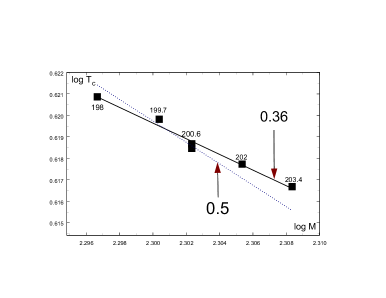
Figure 11: The isotope effect in mercury. The solid line is obtained by the sparse-squares technique. In accordance with the phonon mechanism, the coefficient $\mathfrak{a}$ must be about 1/2 (the dotted line). As it can be seen, this coefficient is in reality approximately equal to 1/3.

2 Superfluidity as a sequence of ordering of zero-point oscillations

2.1 Zero-point oscillation of He atoms and superfluidity

The main features of superfluidity of liquid helium became clear few decades ago [22], [23]. L.D.Landau explains this phenomenon as the manifestation of a quantum behavior of the macroscopic object.

However, the causes and mechanism of the formation of superfluidity are not clear till our days. There is no explanation why the $\lambda$-transition in helium-4 occurs at about 2 K, that is about twice less than its boiling point:

$$\frac{T_{boiling}}{T_{\lambda}}\approx 1.94,$$ (93)

while for helium-3, this transition is observed only at temperatures about a thousand times smaller.

The related phenomenon, superconductivity, can be regarded as superfluidity of a charged liquid. It can be quantitatively described considering it as the consequence of ordering of zero-point oscillations of electron gas. Therefore it seems appropriate to consider superfluidity from the same point of view.

Atoms in liquid helium-4 are electrically neutral, as they have no dipole moments and do not form molecules. Yet some electromagnetic mechanism should be responsible for phase transformations of liquid helium (as well as in other condensed substance where phase transformations are related to the changes of energy of the same scale).

F. London has demonstrated already in the 1930’s [24], that there is an interaction between atoms in the ground state, and this interaction is of a quantum nature. It can be considered as a kind of the Van-der-Waals interaction. Atoms in their ground state (T = 0) perform zero-point oscillations. F.London was considering vibrating atoms as three-dimensional oscillating dipoles which are connected to each other by the electromagnetic interaction. He proposed the name the dispersion interaction for this interaction of atoms in the ground state.

2.2 The dispersion effect in interaction of atoms in the ground state

Following F.London [24], let us consider two spherically symmetric atoms without non-zero average dipole moments. Let us suppose that at some time the charges of these atoms are fluctuationally displaced from the equilibrium states:

$$r_{1}=(x_{1},y_{1},z_{1})$$

$$r_{2}=(x_{2},y_{2},z_{2})$$

If atoms are located along the Z-axis at the distance $L$ of each other, their potential energy can be written as:

$$\mathcal{H}=\underbrace{\frac{e^{2}r_{1}^{2}}{2a}+\frac{e^{2}r_{2}^{2}}{2a}}_{elastic~{}dipoles~{}energy}+\underbrace{\frac{e^{2}}{L^{3}}(x_{1}x_{2}+y_{1}y_{2}-2z_{1}z_{2})}_{elastic~{}dipoles~{}interaction}.$$ (94)

where $a$ is the atom polarizability.

The Hamiltonian can be diagonalized by using the normal coordinates of symmetric and antisymmetric displacements:

$$r_{s}\equiv\left\{\begin{array}[]{ll}x_{s}=\frac{1}{\sqrt{2}}(x_{1}+x_{2})\\ y_{s}=\frac{1}{\sqrt{2}}(y_{1}+y_{2})\\ z_{s}=\frac{1}{\sqrt{2}}(z_{1}+z_{2})\\ \end{array}\right.$$

and

$$r_{a}\equiv\left\{\begin{array}[]{ll}x_{a}=\frac{1}{\sqrt{2}}(x_{1}-x_{2})\\ y_{a}=\frac{1}{\sqrt{2}}(y_{1}-y_{2})\\ z_{a}=\frac{1}{\sqrt{2}}(z_{1}-z_{2})\\ \end{array}\right.$$

This yields

$$\begin{array}[]{ll}x_{1}=\frac{1}{\sqrt{2}}(x_{s}+x_{a})\\ y_{1}=\frac{1}{\sqrt{2}}(y_{s}+y_{a})\\ z_{1}=\frac{1}{\sqrt{2}}(z_{s}+z_{a})\\ \end{array}$$

and

$$\begin{array}[]{ll}x_{2}=\frac{1}{\sqrt{2}}(x_{s}-x_{a})\\ y_{2}=\frac{1}{\sqrt{2}}(y_{s}-y_{a})\\ z_{2}=\frac{1}{\sqrt{2}}(z_{s}-z_{a})\\ \end{array}$$

As the result of this change of variables we obtain:

$$\mathcal{H}=\frac{e^{2}}{2a}(r_{s}^{2}+r_{a}^{2})+\frac{e^{2}}{2L^{3}}(x_{s}^{2}+y_{s}^{3}-2z_{s}^{2}-x_{a}^{2}-y_{a}^{2}+2z_{a}^{2})=$$

$$=\frac{e^{2}}{2a}\left[\left(1+\frac{a}{L^{3}}\right)(x_{s}^{2}+y_{s}^{2})+\left(1-\frac{a}{L^{3}}\right)(x_{a}^{2}+y_{a}^{2})+\right.$$ (95)

$$+\left(1-2\frac{a}{L^{3}}\right)z_{s}^{2}+\left.\left(1+2\frac{a}{L^{3}}\right)z_{a}^{2}\right].$$

Consequently, frequencies of oscillators depend on their orientation and they are determined by the equations:

$$\Omega_{0x}^{s\atop a}=\Omega_{0y}^{s\atop a}=\Omega_{0}\sqrt{1\pm\frac{a}{L^{3}}}\approx\Omega_{0}\left({1\pm\frac{a}{L^{3}}}-\frac{a^{2}}{8L^{6}}\pm...\right)$$ (96)

$$\Omega_{0z}^{s\atop a}=\Omega_{0}\sqrt{1\mp\frac{2a}{L^{3}}}\approx\Omega_{0}\left({1\mp\frac{a}{L^{3}}}-\frac{a^{2}}{2L^{6}}\mp...\right),$$ (97)

where

$$\Omega_{0}=\frac{2\pi e}{\sqrt{ma}}$$ (98)

is natural frequency of the electronic shell of the atom (at $L\rightarrow\infty$). The energy of zero-point oscillations is

$$\mathcal{E}=\frac{1}{2}\hbar(\Omega_{0}^{s}+\Omega_{0}^{a})$$ (99)

It is easy to see that the description of interactions between neutral atoms do not contain terms $\frac{1}{L^{3}}$, which are characteristics for the interaction of zero-point oscillations in the electron gas (Eq.(7)) and which are responsible for the occurrence of superconductivity.
The terms that are proportional to $\frac{1}{L^{6}}$ manifest themselves in interactions of neutral atoms.

It is important to emphasize that the energies of interaction are different for different orientations of zero-point oscillations. So the interaction of zero-point oscillations oriented along the direction connecting the atoms leads to their attraction with energy:

$$\mathcal{E}_{z}=-\frac{1}{2}\hbar\Omega_{0}\frac{A^{2}}{L^{6}},$$ (100)

while the summary energy of the attraction of the oscillators of the perpendicular directions (x and y) is equal to one half of it:

$$\mathcal{E}_{x+y}=-\frac{1}{4}\hbar\Omega_{0}\frac{A^{2}}{L^{6}}$$ (101)

(the minus sign is taken here because for this case the opposite direction of dipoles is energetically favorable).

2.3 The estimation of main characteristic parameters of superfluid helium

2.3.1 The main characteristic parameters of the zero-point oscillations of atoms in superfluid helium-4

There is no repulsion in a gas of neutral bosons. Therefore, due to attraction between the atoms at temperatures below

$$T_{boil}=\frac{2}{3k}\mathcal{E}_{z}$$ (102)

this gas collapses and a liquid forms.

At twice lower temperature

$$T_{\lambda}=\frac{2}{3k}\mathcal{E}_{x+y}$$ (103)

all zero-point oscillations become ordered. It creates an additional attraction and forms a single quantum ensemble.

A density of the boson condensate is limited by zero-point oscillations of its atoms. At condensation the distances between the atoms become approximately equal to amplitudes of zero-point oscillations.

Coming from it, we can calculate the basic properties of an ensemble of atoms with ordered zero-point oscillations, and compare them with measurement properties of superfluid helium.

We can assume that the radius of a helium atom is equal to the Bohr radius $a_{B}$, as it follows from quantum-mechanical calculations. Therefore, the energy of electrons on the s-shell of this atom can be considered to be equal:

$$\hbar\Omega_{0}=\frac{4e^{2}}{a_{B}}$$ (104)

As the polarizability of atom is approximately equal to its volume [25]

$$A\simeq a_{B}^{3},$$ (105)

the potential energy of dispersive interaction (101), which causes the ordering zero-point oscillations in the ensemble of atoms, we can represent by the equation:

$$\mathcal{E}_{x+y}=-\frac{e^{2}}{a_{B}}a_{B}^{6}n^{2},$$ (106)

where the density of helium atoms

$$n=\frac{1}{L^{3}}$$ (107)

2.3.2 The velocity of zero-point oscillations of helium atom

It is naturally to suppose that zero-point oscillations of atoms are harmonic and the equality of kinetic and potential energies are characteristic for them:

$$\frac{M_{4}\widehat{v_{0}}^{2}}{2}-\frac{e^{2}}{a_{B}}a_{B}^{6}n^{2}=0,$$ (108)

where $M_{4}$ is mass of helium atom, $\widehat{v_{0}}$ is their averaged velocity of harmonic zero-point oscillations.

Hence, after simple transformations we obtain:

$$\widehat{v_{0}}=c\alpha^{3}\left\{\frac{n}{n_{0}}\right\},$$ (109)

where the notation is introduced:

$$n_{0}=\frac{\alpha^{2}}{a_{B}^{3}}\sqrt{\frac{M_{4}}{2m_{e}}}.$$ (110)

If the expression in the curly brackets

$$\frac{n}{n_{0}}=1,$$ (111)

we obtain

$$\widehat{v_{0}}=c\alpha^{3}\cong 116.5~{}m/s.$$ (112)

2.3.3 The density of liquid helium

The condition (111) can be considered as the definition of the density of helium atoms in the superfluid state:

$$n=n_{0}=\frac{\alpha^{2}}{a_{B}^{3}}\sqrt{\frac{M_{4}}{2m_{e}}}\cong 2.172\cdot 10^{22}~{}atom/cm^{3}.$$ (113)

According to this definition, the density of liquid helium-4

$$\gamma_{4}=nM_{4}\cong 0.144~{}g/cm^{3}$$ (114)

that is in good agreement with the measured density of the liquid helium $0.145~{}g/cm^{3}$ for $T\simeq T_{\lambda}$.

Similar calculations for liquid helium-3 gives the density $0.094~{}g/cm^{3}$, which can be regarded as consistent with its density $0.082~{}g/cm^{3}$ experimentally measured near the boiling point.

2.3.4 The dielectric constant of liquid helium

To estimate the dielectric constant of helium we can use the Clausius-Mossotti equation [25]:

$$\frac{\varepsilon-1}{\varepsilon+2}=\frac{4\pi}{3}{n}{A}.$$ (115)

At taking into account Eq.(105), we obtain

$$\varepsilon\approx 1.040,$$ (116)

that differs slightly from the dielectric constant of the liquid helium, measured near the $\lambda$-point [28]:

$$\varepsilon\approx 1.057$$ (117)

2.3.5 The temperature of $\lambda$-point

The superfluidity is destroyed at the temperature $T_{\lambda}$, at which the energy of thermal motion is compared with the energy of the Van-der-Waals bond in superfluid condensate

$$\frac{3}{2}kT_{\lambda}-\frac{e^{2}}{a_{B}}a_{B}^{6}n^{2}=0.$$ (118)

With taking into account Eq.(113)

$$T_{\lambda}=\frac{1}{3k}\frac{M_{4}}{m_{e}}\frac{\alpha^{4}e^{2}}{a_{B}}$$ (119)

or after appropriate substitutions

$$T_{\lambda}=\frac{1}{3}\frac{M_{4}c^{2}\alpha^{6}}{k}=2.177K,$$ (120)

that is in very good agreement with the measured value $T_{\lambda}=2.172K$.

2.3.6 The boiling temperature of liquid helium

After comparison of Eq.(100) - Eq.(101), we have

$$T_{boil}=2T_{\lambda}=4.35K$$ (121)

This is the basis for the assumption that the liquefaction of helium is due to the attractive forces between the atoms with ordered lengthwise components of their oscillations.

2.3.7 The velocity of the first sound in liquid helium

It is known from the theory of the harmonic oscillator that the maximum value of its velocity is twice bigger than its average velocity. In this connection, at assumption that the first sound speed $c_{s1}$ is limited by this maximum speed oscillator, we obtain

$$c_{s1}=2\widehat{v_{0}}\simeq 233~{}m/s.$$ (122)

It is in consistent with the measured value of the velocity of the first sound in helium, which has the maximum value of $238.3~{}m/s$ at $T\rightarrow 0$ and decreases with increasing temperature up to about $220~{}m/s$ at $T=T_{\lambda}$.

The results obtained in this subsection are summarized for clarity in the Table.(8).

The measurement data in this table are mainly quoted by [27] and [28].

	defining	calculated	measured
parameter
	formula	value	value
the velocity of zero-point
oscillations of	$\widehat{v_{0}}=c\alpha^{3}$	$116.5$
helium atom		m/s
The density of atoms
in liquid	$n=\sqrt{\frac{M_{4}}{2m_{e}}}\frac{\alpha^{2}}{a_{B}^{3}}$	$2.172\cdot 10^{22}$
helium		$atom/cm^{3}$
The density
of liquid helium-4	$\gamma=M_{4}n$	$144.3$	$145_{T\simeq T_{\lambda}}$
$g/l$
The dielectric			$1.048_{T\simeq 4.2}$
constant	$\frac{\varepsilon-1}{\varepsilon+2}=\frac{4\pi}{3}{\alpha^{2}}{\sqrt{\frac{M_{4}}{2m_{e}}}}$	1.040
of liquid helium-4			$1.057_{T\simeq T_{\lambda}}$
The temperature
	$T_{\lambda}\simeq\frac{M_{4}c^{2}\alpha^{6}}{3}$	$2.177$	$2.172$
$\lambda$-point,K
The boiling
temperature	$T_{boil}\simeq 2T_{\lambda}$	$4.35$	$4.21$
of helium-4,K
The first sound
velocity,	$c_{s1}=2\widehat{v_{0}}$	$233$	$238.3_{T\rightarrow 0}$
$m/s$

Table 8: Comparison of the calculated values of liquid helium-4 with the measurement data

2.3.8 The estimation of characteristic properties of He-3

The results of similar calculations for the helium-3 properties are summarized in the Tab.(9).

	defining	calculated	measured
parameter
	formula	value	value
The velocity of zero-point
oscillations of	$\widehat{v_{0}}=c\alpha^{3}$	$116.5$
helium atom		m/s
The density of atoms
in liquid	$n_{3}=\sqrt{\frac{M_{3}}{2m_{e}}}\frac{\alpha^{2}}{a_{B}^{3}}$	$1.88\cdot 10^{22}$
helium-3		$atom/cm^{3}$
The density
of liquid	$\gamma=M_{3}n_{3}$	$93.7~{}$	$82.3~{}$
helium-3, g/l
The dielectric
constant	$\frac{\varepsilon-1}{\varepsilon+2}=\frac{4\pi}{3}{\alpha^{2}}{\sqrt{\frac{M_{3}}{2m_{e}}}}$	1.035
of liquid helium-3
The boiling
temperature	$T_{boil}\simeq\frac{4}{3}\frac{\mathcal{E}_{W}}{k}$	$3.27$	$3.19$
of helium-3,K
The sound velocity
in liquid	$c_{s}=2\widehat{v_{0}}$	233
helium-3		m/s

Table 9: The characteristic properties of liquid helium-3

There is a radical difference between mechanisms of transition to the superfluid state for He-3 and He-4. Superfluidity occurs if complete ordering exists in the atomic system. For superfluidity of He-3 electromagnetic interaction should order not only zero-point vibrations of atoms, but also the magnetic moments of the nuclei.

It is important to note that all characteristic dimensions of this task: the amplitude of the zero-point oscillations, the atomic radius, the distance between atoms in liquid helium - all equal to the Bohr radius $a_{B}$ by the order of magnitude. Due to this fact, we can estimate the oscillating magnetic field, which a fluctuating electronic shell creates on ”its”  nucleus:

$$H_{\Omega}\approx\frac{e}{a_{B}^{2}}\frac{a_{B}\Omega_{0}}{c}\approx\frac{\mu_{B}}{A_{3}},$$ (123)

where $\mu_{B}=\frac{e\hbar}{2m_{e}c}$ is the Bohr magneton, $A_{3}$ is the electric polarizability of helium-3 atom.

Because the value of magnetic moments for the nuclei He-3 is approximately equal to the nuclear Bohr magneton $\mu_{n_{B}}=\frac{e\hbar}{2m_{p}c}$, the ordering in their system must occur below the critical temperature

$$T_{c}=\frac{\mu_{n_{B}}H_{\Omega}}{k}\approx 10^{-3}K.$$ (124)

This finding is in agreement with the measurement data. The fact that the nuclear moments can be arranged in parallel or antiparallel to each other is consistent with the presence of the respective phases of superfluid helium-3.

Concluding this approach permits to explain the mechanism of superfluidity in liquid helium.

In this way, the apposite quantitative estimations of main parameters of the liquid helium and its transition to the superfluid state were obtained.

It was established that both related phenomena, superconductivity and superfluidity, are based on the same physical mechanism: they both are consequences of the ordering of zero-point oscillations.

3 Conclusion

Until now it has been commonly thought that the existence of the isotope effect in superconductors leaves only one way for explanation of the superconductivity phenomenon - the way based on the phonon mechanism.

Over fifty years of theory development based on the phonon mechanism, has not lead to success. All attempts to explain why some superconductors have certain critical temperatures (and critical magnetic fields) have failed.

This problem was further exacerbated with the discovery of high temperature superconductors. How can we move forward in HTSC understanding, if we cannot understand the mechanism that determines the critical temperature elementary superconductors?

In recent decades, experimenters have shown that isotopic substitution in metals leads to a change in the parameters of their crystal lattice and thereby affect the Fermi energy of the metal. As results, the superconductivity can be based on a nonphonon mechanism.

The theory proposed in this paper suggests that the specificity of the association mechanism of electrons pairing is not essential. It is merely important that such a mechanism was operational over the whole considered range of temperatures. The nature of the mechanism forming the electron pairs does not matter, because although the work of this mechanism is necessary it is still not a sufficient condition for the superconducting condensate’s existence. This is caused by the fact that after the electron pairing, they still remain as non-identical particles and cannot form the condensate, because the individual pairs differ from each other as they commit uncorrelated zero-point oscillations. Only after an ordering of these zero-point oscillations, an energetically favorable lowering of the energy can be reached and a condensate at the level of minimum energy can then be formed. Due to this reason the ordering of zero-point oscillations must be considered as the cause of the occurrence of superconductivity.

Therefore, the density of superconducting carriers and the critical temperature of a superconductor are determined by the Fermi energy of the metal, The critical magnetic field of a superconductor is given by the mechanism of destruction of the coherence of zero-point oscillations.

In conclusion, the consideration of zero-point oscillations allows us to construct the theory of superconductivity, which is characterized by the ability to give estimations for the critical parameters of elementary superconductors. These results are in satisfactory agreement with measured data.

This approach permit to explain the mechanism of superfluidity in liquid helium. For electron shells of atoms in S-states, the energy of interaction of zero-point oscillations can be considered as a manifestation of Van-der-Waals forces. In this way the apposite quantitative estimations of temperatures of the helium liquefaction and its transition to the superfluid state was obtained.

Thus it is established that both related phenomena, superconductivity and superfluidity, are based on the same physical mechanism - they both are consequences of the ordering of zero-point oscillations.

References

- [1] Maxwell E. : Phys.Rev.,,p 477(1950)
- [2] Serin et al : Phys.Rev.B,,p 813(1950)
- [3] Inyushkin A.V. : Section 12 in ”Isotops” (Editor Baranov V.Yu), PhysMathLit, 2005 (In Russian)
- [4] Vasiliev B.V. : Physica C, 471,277-284 (2011)
- [5] Vasiliev B.V. : Physica C, 471,277-284 (2012)
- [6] Vasiliev B.V. : ”Superconductivity, Superfluidity and Zero-Point Oscillations” in ”Recent Advances in Superconductivity Research” , pp.249-280, Nova Publisher,NY(2013)
- [7] Bardeen J.: Phys.Rev.,,p. 167-168(1950).
- [8] Shablo A.A. et al: Letters JETPh, v.19, 7,p.457-461 (1974)
- [9] Sharvin D.Iu. and Sharvin Iu.V.: Letters JETPh, v.34, 5, p.285-288 (1981)
- [10] Vasiliev B.V. and Luboshits V.L.: , 345, (1994)
- [11] Ketterson J.B. and Song S.N.: Superconductivity, Cambridge (1999)
- [12] Pool Ch.P.Jr : Handbook of Superconductivity, Academic Press, (2000)
- [13] Landau L.D. and Lifshits E.M.: Statistical Physics, 1, 3rd edition, Oxford:Pergamon, (1980)
- [14] Kittel Ch. : Introduction to Solid State Physics, Wiley (2005)
- [15] Linton E.A. : Superconductivity, London: Mathuen and Co.LTDA, NY: John Wiley and Sons Inc., (1964)
- [16] Abragam-Becker : Teorie der Elektizität, Band 1, Leupzig-Berlin, (1932)
- [17] Albert Messiah: Quantum Mechanics (Vol. II), North Holland, John Wiley and Sons. (1966)
- [18] Ashcroft N.W., Mermin N.D.: Solid state physics, v 2., Holt,Rinehart and Winston, (1976)
- [19] Golovashkin A.I. : Preprint PhIAN, 10, Moscou, 2005 (in Russiian).
- [20] Kogan V.S.: Physics-Uspekhi, 579 (1962)
- [21] Wang D.T. et al : Phys.Rev.B,,N 20,p. 13167(1997)
- [22] Landau L.D. : JETP, 11, 592 (1941)
- [23] Khalatnikov I.M.: Introduction into theory of superfluidity, Moscow, Nauka, (1965)
- [24] London F.: Trans. Faraday Soc. 33, p.8 (1937)
- [25] Fröhlich H. : Theory of dielectrics, Oxford, (1957)
- [26] Ilianok A.M: Eurasian patent № 003164, US patent 6,570,224B1, Korean patent N 10-0646267, China patent CN 1338120.
- [27] Kikoine I.K. a.o.: Physical Tables, Moscow, Atomizdat (1978) (in Russian).
- [28] Russel J.Donnelly and Carlo F.Barenghy: The Observed Properties of Liquid Helium, Journal of Physical and Chemical Data, , N1, pp.51-104, (1977)