Analytical thermodynamics of a strongly attractive three-component Fermi gas in one dimension

Abstract

Ultracold three-component atomic Fermi gases in one dimension are expected to exhibit rich physics due to the presence of trions and different pairing states. Quantum phase transitions from the trion state into a paired phase and a normal Fermi liquid occur at zero temperature. We derive the analytical thermodynamics of strongly attractive three-component one-dimensional fermions with $SU(3)$ symmetry via the thermodynamic Bethe ansatz method in unequal Zeeman splitting fields $H_{1}$ and $H_{2}$. We find explicitly that for low temperature the system acts like either a two-component or a three-component Tomonaga-Luttinger liquid dependent on the system parameters. The phase diagrams for the chemical potential and specific heat are presented for illustrative values of the Zeeman splitting. We also demonstrate that crossover between different Tomonaga-Luttinger liquid phases exhibit singular behaviour in specific heat and entropy as the temperature tends to zero. Beyond Tomonaga-Luttinger liquid physics, we obtain the equation of state which provides a precise description of universal thermodynamics and quantum criticality in three-component strongly attractive Fermi gases.

I Introduction

The ongoing experimental advances in realizing degenerate quantum gases in low dimensions TGexp ; Toshiya ; Moritz05 ; Druten ; Haller ; Hulet offer a new and compelling motivation for the further study of quantum many-body systems via exact schemes such as the Bethe Ansatz (BA) and low energy effective field theory Giamarchi-b . Reducing the dimensionality in a quantum system can have striking consequences. The one-dimensional (1D) many-body systems Giamarchi-b ; Takahashi possess unique many-body correlation effects which are different from their higher dimensional counterparts. These include the phenomena of spin-charge separation, universal thermodynamics and quantum criticality.

A recent scheme for mapping out physical properties of homogeneous systems by using the inhomogeneity of the trap Ho-Zhou has been successfully applied to experimental measurements on the thermodynamics of interacting fermions with a wide range of tunable interactions Salomon ; Horikoshi . Moreover, further experimental advances with ultracold atoms allow the exploration of three-component Fermi gases in the entire parameter space of trions, dimers and free atoms Li ; efimov-trimer ; Li2 . This provides a promising opportunity to experimentally explore universal thermodynamics and quantum critical behaviour of strongly interacting Fermi gases with high spin symmetries in 1D. In this context, the thermodynamics of 1D attractively interacting fermions Takahashi has been receiving growing interest Guan2007prb ; Mueller ; Bolech ; Erhai .

For spin-1/2 fermions with attractive interaction there are three quantum phases at zero temperature: the fully paired phase which is a quasi-condensate with zero polarization $p$, the fully polarized (normal) phase with $p=1$, and the partially polarized (1D FFLO) phase where $0<p<1$ at zero temperature Orso ; Hu ; Guan2007prb . This theoretical prediction of the phase diagram for 1D fermions was recently confirmed experimentally by R. Hulet’s group at Rice University Hulet . In addition, it was recently proved Erhai that at low temperatures, the physics of the gapless phase belongs to the universality class of a two-component Tomonaga-Luttinger liquid (TLL). However, from the theoretical point of view, understanding the thermodynamics of multi-component Fermi gases with higher spin symmetry imposes a number of challenges Ho ; Tsvelik ; Zhang ; Wang ; Guan .

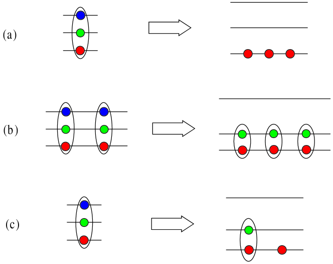
Figure 1: (Color online) Phase transitions from states of trions into (a) normal Fermi liquid, (b) fully-paired states and (c) the mixture of pairs and unpaired fermions. The transitions are induced by linear (a) and nonlinear ((b) and (c)) Zeeman splitting. Ellipses denote charge bound states.

For multi-component interacting Fermi gases, the phase diagrams become more complicated in the presence of magnetic fields due to the richer number of quantum phases. In contrast to the two-component Fermi gas, Orso ; Hu ; Guan2007prb three-component ultracold fermions give rise to quantum phase transitions from a three-body bound state of “trions” into the BCS pairing state and a normal Fermi liquid Rapp ; Lecheminant ; Demler ; Guan2008prl ; Thai ; Silva ; Errea ; AnnPhys ; Suga2009arXiv ; Angela . The zero temperature phase diagrams of the BA integrable 1D three-component Fermi gas with $SU(3)$ symmetry have been worked out from the dressed energy equations Guan2008prl ; Angela . It was found that Zeeman splittings can drive transitions between exotic phases of trions, bound pairs, a normal Fermi liquid and mixtures of these phases, see Fig. 1. It is thus very worthwhile to map out such zero temperature phase diagrams to the inhomogeneity of the trap at finite temperatures.

In this paper, we investigate the finite temperature thermodynamic properties of 1D three-component fermions with unequal Zeeman splitting by means of the exact thermodynamic Bethe ansatz (TBA) solution. We prove that at low temperatures the system behaves like either a two-component or a three-component TLL in certain regimes. Exact finite temperature phase diagrams are demonstrated for illustrative values of the Zeeman splitting parameters. Quantum criticality with respect to the specific heat and entropy as the temperature tends to zero is discussed. The equation of state obtained provides an exact description of the thermodynamics and quantum critical behaviour of three-component composite fermions which can possibly be tested in experiments with ultracold atoms.

This paper is set out as follows. In Section II, we present the model and the exact BA solution. We also derive the TBA equations for the thermodynamics. In Section III, we derive the low temperature thermodynamics by the Sommerfeld expansion method. The universal multi-component TLL phases are identified. In Section IV, we present the equation of state in terms of polylogarithm functions from which the quantum phase diagrams can be mapped out. Concluding remarks are given in Section V. Detailed working is given in the appendices. The derivation of the TBA equations is presented in detail in Appendix A. In Appendices B and C, the iteration method is used to derive relevant results for the TBA and the thermodynamics.

II The Model and the thermodynamic Bethe ansatz solution

We consider a 1D system of $N$ fermions of mass $m$ with spin independent $\delta$-function potential interaction and are constrained to a line of length $L$ with periodic boundary conditions. The fermions can occupy three possible hyperfine levels ($\left|1\right\rangle$, $\left|2\right\rangle$ and $\left|3\right\rangle$) with particle number $N^{1}$, $N^{2}$ and $N^{3}$, respectively. The system can be described by the Hamiltonian Sutherland ; Takahashi-2

$$\mathcal{H}_{0}=-\frac{\hbar^{2}}{2m}\sum_{i=1}^{N}\frac{\partial^{2}}{\partial x_{i}^{2}}+g_{1D}\sum_{1\leq i<j\leq N}\delta(x_{i}-x_{j})+E_{Z}$$ (1)

where we have included the Zeeman energy $E_{Z}=\sum_{i=1}^{3}N^{i}\epsilon^{i}_{Z}(\mu_{B}^{i},B)$. The spin-independent contact interaction $g_{\rm 1D}$ applies between fermions with different hyperfine states so that the number of fermions in each spin state is conserved. The inter-component interaction $g_{1D}$ is positive for repulsive interaction and negative for attractive interaction. For simplicity, we define the interaction strengths as $c=mg_{1D}/\hbar^{2}$ and the dimensionless parameter $\gamma=c/n$, where $n=N/L$ is the linear density, and set $\hbar=2m=1$. Although these conditions appear rather restrictive, it is possible to tune scattering lengths between atoms in different low sublevels to form nearly $SU(3)$ degeneracy Fermi gases via broad Feshbach resonances Li ; efimov-trimer ; Li2 .

In the above equation, the Zeeman energy levels $\epsilon^{i}_{Z}$ are determined by the magnetic moments $\mu_{B}^{i}$ and the magnetic field $B$. By convention, particle numbers in each of the hyperfine states satisfy the relation $N^{1}\geq N^{2}\geq N^{3}$. Thus the particle numbers of unpaired fermions, pairs, and trions are respectively given by $N_{1}=N^{1}-N^{2}$, $N_{2}=N^{2}-N^{3}$ and $N_{3}=N^{3}$ for the attractive regime.

In order to simplify calculations in the study of population imbalance, we rewrite the Zeeman energy as $E_{Z}=-H_{1}N_{1}-H_{2}N_{2}+N\bar{\epsilon}$ where the unequally spaced Zeeman splitting in three hyperfine levels can be characterized by two independent parameters $H_{1}=\bar{\epsilon}-\epsilon^{1}_{Z}(\mu_{B}^{1},B)$ and $H_{2}=\epsilon^{3}_{Z}(\mu_{B}^{3},B)-\bar{\epsilon}$, with $\bar{\epsilon}=\sum_{i=1}^{3}\epsilon^{i}_{Z}(\mu_{B}^{i},B)/3$ the average Zeeman energy. Pure Zeeman splitting (equally-spaced splitting), i.e. $H_{1}=H_{2}$, leads to a smooth phase transition from trions into the normal Fermi liquid. On the other hand, unequally-spaced Zeeman splitting can lead to quantum phase transitions from trions to the fully-paired phase and to a mixture of pairs and single atoms, see Fig. 1.

The Hamiltonian (1) exhibits a symmetry of $U(1)\times SU(3)$, where $U(1)$ and $SU(3)$ describe the charge and spin degrees of freedom. This model was solved long ago by means of the nested Bethe ansatz Sutherland ; Takahashi-2 . The energy eigenspectrum is given in terms of the quasimomenta $\left\{k_{j}\right\}$ of the $N$ fermions by

$$E=\sum_{j=1}^{N}k_{j}^{2}$$ (2)

which satisfy the BA equations Sutherland ; Takahashi-2

$$e^{\mathrm{i}k_{j}L} = \prod_{\ell=1}^{M_{1}}\frac{k_{j}-\Lambda_{\ell}+\mathrm{i}c/2}{k_{j}-\Lambda_{\ell}-\mathrm{i}c/2},$$

$$\prod_{j=1}^{N}\frac{\Lambda_{\ell}-k_{j}+\mathrm{i}c/2}{\Lambda_{\ell}-k_{j}-\mathrm{i}c/2} = -\prod_{\alpha=1}^{M_{1}}\frac{\Lambda_{\ell}-\Lambda_{\alpha}+\mathrm{i}c}{\Lambda_{\ell}-\Lambda_{\alpha}-\mathrm{i}c}$$

$$\times\prod_{m=1}^{M_{2}}\frac{\Lambda_{\ell}-\lambda_{m}-\mathrm{i}c/2}{\Lambda_{\ell}-\lambda_{m}+\mathrm{i}c/2},$$

$$\prod_{\ell=1}^{M_{1}}\frac{\lambda_{m}-\Lambda_{\ell}+\mathrm{i}c/2}{\lambda_{m}-\Lambda_{\ell}-\mathrm{i}c/2} = -\prod_{\beta=1}^{M_{2}}\frac{\lambda_{m}-\lambda_{\beta}+\mathrm{i}c}{\lambda_{m}-\lambda_{\beta}-\mathrm{i}c}.$$ (3)

Here $j=1,\ldots,N$, $\ell=1,\ldots,M_{1}$, $m=1,\ldots,M_{2}$ with quantum numbers $M_{1}=N^{2}+N^{3}$ and $M_{2}=N^{3}$. The parameters $\left\{\Lambda_{\ell},\lambda_{m}\right\}$ are the rapidities for the internal hyperfine spin degree of freedom.

In the thermodynamic limit, $N,L\rightarrow\infty$ with $n$ finite, the sets of solutions $\{k_{j}\}$, $\{\Lambda_{\ell}\}$ and $\{\lambda_{m}\}$ of the BA equations (3) are of certain forms, as discussed in Appendix A. For attractive interaction the quasimomenta $\{k_{j}\}$ can form two-body and three-body charge bound states, which give a natural description of composite fermions, and can also be real Takahashi-2 ; Guan2008prl . However, the rapidities $\{\Lambda_{\ell}\}$ and $\{\lambda_{m}\}$ can form complex spin-strings characterizing the spin wave fluctuations at finite temperatures.

In the thermodynamic limit, the grand partition function Yang1969 ; Takahashi $Z=\mathrm{tr}(\mathrm{e}^{-H/T})=\mathrm{e}^{-G/T}$ is given in terms of the Gibbs free energy

$$G = E-\mu N+E_{\rm Z}-TS$$ (4)

$$= E-\mu N-H_{1}N_{1}-H_{2}N_{2}-TS,$$

where the chemical potential $\mu$, the Zeeman energy $E_{\rm Z}$ and the entropy $S$ are given in terms of the densities of unpaired fermions, charge bound states, trions and spin-strings, which are all subject to the BA equations (3). The equilibrium states are determined by minimizing the Gibbs free energy, which gives rise to a set of coupled nonlinear integral equations – the TBA equations for the dressed energies $\varepsilon_{a}(a=1,2,3)$, which are derived for this model in Appendix A, with final result

$$\varepsilon_{1}(k) = k^{2}-\mu-H_{1}+\,Ta_{1}\ast\ln(1+e^{-{\varepsilon_{2}}/{T}})(k)$$

$$+\,Ta_{2}\ast\ln(1+e^{-\varepsilon_{3}/T})(k)$$

$$-\,T\sum_{n=1}^{\infty}a_{n}\ast\ln(1+\xi_{n}^{-1})(k),$$

$$\varepsilon_{2}(k) = 2k^{2}-\frac{1}{2}{c^{2}}-2\mu-H_{2}$$

$$+\,Ta_{1}\ast\ln(1+e^{-{\varepsilon_{1}}/{T}})(k)$$

$$+\,Ta_{2}\ast\ln(1+e^{-{\varepsilon_{2}}/T})(k)$$

$$+\,T(a_{1}+a_{3})\ast\ln(1+e^{-{\varepsilon_{3}}/T})(k)$$

$$-\,T\sum_{n=1}^{\infty}a_{n}\ast\ln(1+\zeta_{n}^{-1})(k),$$

$$\varepsilon_{3}(k) = 3k^{2}-2{c^{2}}-3\mu+Ta_{2}\ast\ln(1+e^{-\varepsilon_{1}/T})(k)$$ (5)

$$+\,T(a_{1}+a_{3})\ast\ln(1+e^{-{\varepsilon_{2}}/{T}})(k)$$

$$+\,T(a_{2}+a_{4})\ast\ln(1+e^{-{\varepsilon_{3}}/{T}})(k).$$

Here the quantity

$$a_{m}\left(x\right)=\frac{1}{2\pi}\frac{m\left|c\right|}{\left(mc/2\right)^{2}+x^{2}}$$ (6)

and $\ast$ denotes the convolution,

$$(a\ast b)(x)=\int a(x-y)b(y)dy.$$ (7)

The spin string parameters $\xi_{n}:=\sigma_{n}^{h}/\sigma_{n}$ and $\zeta_{n}:=\tau_{n}^{h}/\tau_{n}$ associated with particle and hole densities of string length $n$ in $\Lambda$ and $\lambda$ parameter spaces satisfy the string TBA equations

$$\ln\xi_{n}\left(\Lambda\right) = \frac{n(2H_{1}-H_{2})}{T}+a_{n}\ast\ln(1+e^{-{\varepsilon_{1}}/{T}})\left(\Lambda\right)$$

$$+\sum_{m}T_{mn}\ast\ln(1+\xi_{m}^{-1})\left(\Lambda\right)$$

$$-\sum_{m}S_{mn}\ast\ln(1+\zeta_{m}^{-1})\left(\Lambda\right),$$

$$\ln\zeta_{n}\left(\lambda\right) = \frac{n(2H_{2}-H_{1})}{T}+a_{n}\ast\ln(1+e^{-{\varepsilon_{2}}/{T}})\left(\lambda\right)$$ (8)

$$+\sum_{m}T_{mn}\ast\ln(1+\zeta_{m}^{-1})\left(\lambda\right)$$

$$-\sum_{m}S_{mn}\ast\ln(1+\xi_{m}^{-1})\left(\lambda\right).$$

The functions $T_{mn}$ and $S_{mn}$ are as defined in Appendix A.

In the thermodynamic limit, the pressure $p$ is defined in terms of the Gibbs energy (4) by $p\equiv-(\partial G/\partial L)$, which includes three parts, $p^{(1)}$, $p^{(2)}$ and $p^{(3)}$, for the pressure of unpaired fermions, pairs and trions, respectively, where

$$p^{(a)}=\frac{aT}{2\pi}\int dk\ln\left(1+e^{-\varepsilon_{a}\left(k\right)/{T}}\right).$$ (9)

Here we have set the Boltzmann constant $k_{B}=1$.

The TBA equations (5) are expressed in terms of the dressed energies $\varepsilon_{1}(k)$, $\varepsilon_{2}(k)$ and $\varepsilon_{3}(k)$ for unpaired fermions, pairs and trions, respectively. The dressed energies are seen to depend not only on the chemical potential $\mu$ and the external fields $H_{1}$ and $H_{2}$ but also on the interactions among themselves as well as the spin fluctuations characterized by the spin-strings (8). We clearly see that spin fluctuations are ferromagnetically coupled to the dressed energies for unpaired fermions and pairs. There is no such spin fluctuation coupled to the dressed energy of the spin neutral trion states. The TBA equations play the central role in the investigation of thermodynamic properties of exactly solvable models at finite temperature. They also provides a convenient formalism to analyze quantum phase transitions and magnetic effects in the presence of external fields at zero temperature review .

III Universal Tomonaga-Luttinger liquid phases

The TBA equations (5) and (8) involve an infinite number of coupled nonlinear integral equations which hinders access to the thermodynamics from both the analytical and numerical points of view. In the strong coupling regime, the dressed energies $\varepsilon_{a}(k)$ with $a=1,\,2,\,3$ marginally depend on each other. The spin string contributions to thermal fluctuations in the strong coupling regime and at low temperatures, i.e. $T\ll H_{1}$ and $T\ll H_{2}$, are negligible. In this temperature regime, the TBA equations (5) can be sorted as

$$\varepsilon_{a}(k) \approx a\,k^{2}-A^{(a)},\qquad a=1,\,2,\,3,$$ (10)

in terms of the dressed chemical potentials

$$A^{(1)} = \mu+H_{1}-\frac{2}{|c|}p^{(2)}-\frac{2}{3|c|}p^{(3)},$$

$$A^{(2)} = 2\mu+\frac{1}{2}{c^{2}}+H_{2}-\frac{4}{|c|}p^{(1)}-\frac{1}{|c|}p^{(2)}-\frac{16}{9|c|}p^{(3)},$$

$$A^{(3)} = 3\mu+2c^{2}-\frac{2}{|c|}p^{(1)}-\frac{8}{3|c|}p^{(2)}-\frac{1}{|c|}p^{(3)}.$$ (11)

In this case we can directly calculate the pressure through (9), with result

$$p^{(a)}=\frac{\sqrt{a}}{\pi}\int_{0}^{\infty}\frac{\sqrt{\varepsilon_{a}}d\varepsilon_{a}}{1+\mathrm{e}^{(\varepsilon_{a}-A^{(a)})/T}}$$ (12)

in terms of chemical potential $\mu$, temperature $T$ and external fields $H_{1}$ and $H_{2}$. Using Sommerfeld expansion, we obtain the pressure $p^{(a)}$ at low temperatures,

$$p^{(a)}\approx\frac{2}{3}\sqrt{\frac{a}{{\pi^{2}}}}\left(A^{(a)}\right)^{\frac{3}{2}}\left[1+\frac{\pi^{2}}{8}\left(\frac{T}{A^{(a)}}\right)^{2}\right].$$ (13)

The fields $H_{1}$ and $H_{2}$ may drive the system into a number of different phases. In order to extract the nature of the TLL physics from the low temperature thermodynamics, we first consider the phase in which trions, pairs and unpaired fermions coexist. In this coexisting phase, we can apply Sommerfeld expansion under the condition that the effective chemical potentials for trions, pairs and unpaired fermions are greater than the temperature scale. Iteration with the defining relations

$$n=\frac{\partial p}{\partial\mu},\,\,\,n_{1}=\frac{\partial p}{\partial H_{1}},\,\,\,n_{2}=\frac{\partial p}{\partial H_{2}},$$ (14)

leads to explicit forms for the pressure

$$p^{(1)} \approx \frac{2n_{1}^{3}\pi^{2}}{3}\left(1+\frac{12n_{2}}{|c|}+\frac{6n_{3}}{|c|}+\frac{\pi^{2}}{4}\left(\frac{T}{n_{1}^{2}{\pi^{2}}}\right)^{2}\left[1-\frac{4n_{2}}{|c|}-\frac{2n_{3}}{|c|}\right]\right),$$ (15)

$$p^{(2)} \approx \frac{n_{2}^{3}\pi^{2}}{3}\left(1+\frac{6n_{1}}{|c|}+\frac{3n_{2}}{|c|}+\frac{8n_{3}}{|c|}+\frac{\pi^{2}}{4}\left(\frac{T}{\frac{n_{2}^{2}}{2}\pi^{2}}\right)^{2}\left[1-\frac{2n_{1}}{|c|}-\frac{n_{2}}{|c|}-\frac{8n_{3}}{3|c|}\right]\right),$$ (16)

$$p^{(3)} \approx \frac{2n_{3}^{3}\pi^{2}}{9}\left(1+\frac{2n_{1}}{|c|}+\frac{16n_{2}}{3|c|}+\frac{3n_{3}}{|c|}+\frac{\pi^{2}}{4}\left(\frac{T}{\frac{n_{3}^{2}}{3}\pi^{2}}\right)^{2}\left[1-\frac{2n_{1}}{3|c|}-\frac{16n_{2}}{9|c|}-\frac{n_{3}}{|c|}\right]\right).$$ (17)

The detailed derivation is given in Appendix B. For the total number of particles fixed, i.e. $n=n_{1}+2n_{2}+3n_{3}$, the free energy can be written as

$$F = \mu n-p$$ (18)

$$= \mu^{(1)}n_{1}+2\mu^{(2)}n_{2}+3\mu^{(3)}n_{3}$$

$$-H_{1}n_{1}-H_{2}n_{2}-\frac{c^{2}}{2}n_{2}-2c^{2}n_{3}-p,$$

where effective chemical potentials $\mu^{(a)}$s are given by

$$\mu^{(1)} = \mu+H_{1},$$ (19)

$$\mu^{(2)} = \mu+\frac{1}{4}{c^{2}}+\frac{1}{2}{H_{2}},$$ (20)

$$\mu^{(3)} = \mu+\frac{2}{3}{c^{2}}.$$ (21)

In order to see universal TLL physics, we calculate the leading low temperature corrections to the free energy $F$. Substituting $\mu^{(a)}$ and $p^{(a)}$ into (18), after some lengthy calculation, we obtain the leading temperature correction to the free energy

$$F\approx E_{0}-\frac{\pi T^{2}}{6}\left(\frac{1}{v_{1}}+\frac{1}{v_{2}}+\frac{1}{v_{3}}\right),$$ (22)

where the ground state energy is given by

$$E_{0}=-H_{1}n_{1}-H_{2}n_{2}-\frac{1}{2}c^{2}n_{2}-2c^{2}n_{3}$$ (23)

and the velocities are

$$v_{1} \approx 2n_{1}\pi\left(1+\frac{8}{|c|}n_{2}+\frac{4}{|c|}n_{3}\right),$$

$$v_{2} \approx 4n_{2}\pi\left(1+\frac{4}{|c|}n_{1}+\frac{2}{|c|}n_{2}+\frac{16}{3|c|}n_{3}\right),$$

$$v_{3} \approx 6n_{3}\pi\left(1+\frac{4}{3|c|}n_{1}+\frac{32}{9|c|}n_{2}+\frac{2}{|c|}n_{3}\right).$$ (24)

The particle numbers $n_{1}$, $n_{2}$ and $n_{3}$ of different bound states can be obtained approximately by collecting terms up to order $1/|c|$ in the expressions for the effective chemical potentials $\mu^{(a)}$ in (19)-(21) at zero temperature,

$$\mu^{(1)} \approx n_{1}^{2}{\pi^{2}}\left(1+\frac{2}{3|c|}\frac{n_{2}^{3}}{n_{1}^{2}}+\frac{4}{27|c|}\frac{n_{3}^{3}}{n_{1}^{2}}+\frac{8}{|c|}n_{2}+\frac{4}{|c|}n_{3}\right),$$ (25)

$$\mu^{(2)} \approx \frac{n_{2}^{2}}{4}\pi^{2}\left(1+\frac{16}{3|c|}\frac{n_{1}^{3}}{n_{2}^{2}}+\frac{64}{81|c|}\frac{n_{3}^{3}}{n_{2}^{2}}+\frac{4}{|c|}n_{1}+\frac{8}{3|c|}n_{2}+\frac{16}{3|c|}n_{3}\right),$$ (26)

$$\mu^{(3)} \approx \frac{n_{3}^{2}}{9}\pi^{2}\left(1+\frac{4}{|c|}\frac{n_{1}^{3}}{n_{3}^{2}}+\frac{8}{3|c|}\frac{n_{2}^{3}}{n_{3}^{2}}+\frac{4}{3|c|}n_{1}+\frac{32}{9|c|}n_{2}+\frac{8}{3|c|}n_{3}\right).$$ (27)

with final result

$$n_{1} \approx \frac{\sqrt{\mu^{(1)}}}{\pi}\left(1-\frac{8}{3\pi|c|}\frac{\left(\mu^{(2)}\right)^{\frac{3}{2}}}{\mu^{(1)}}-\frac{2}{\pi|c|}\frac{\left(\mu^{(3)}\right)^{\frac{3}{2}}}{\mu^{(1)}}-\frac{8}{\pi|c|}\sqrt{\mu^{(2)}}-\frac{6}{\pi|c|}\sqrt{\mu^{(3)}}\right),$$ (28)

$$n_{2} \approx \frac{2\sqrt{\mu^{(2)}}}{\pi}\left(1-\frac{2}{3\pi|c|}\frac{\left(\mu^{(1)}\right)^{\frac{3}{2}}}{\mu^{(2)}}-\frac{8}{3\pi|c|}\frac{\left(\mu^{(3)}\right)^{\frac{3}{2}}}{\mu^{(2)}}-\frac{2}{\pi|c|}\sqrt{\mu^{(1)}}-\frac{8}{3\pi|c|}\sqrt{\mu^{(2)}}-\frac{8}{\pi|c|}\sqrt{\mu^{(3)}}\right),$$ (29)

$$n_{3} \approx \frac{3\sqrt{\mu^{(3)}}}{\pi}\left(1-\frac{2}{9\pi|c|}\frac{\left(\mu^{(1)}\right)^{\frac{3}{2}}}{\mu^{(3)}}-\frac{32}{27\pi|c|}\frac{\left(\mu^{(2)}\right)^{\frac{3}{2}}}{\mu^{(3)}}-\frac{2}{3\pi|c|}\sqrt{\mu^{(1)}}-\frac{32}{9\pi|c|}\sqrt{\mu^{(2)}}-\frac{4}{\pi|c|}\sqrt{\mu^{(3)}}\right).$$ (30)

This result shows that strongly attractive three-component fermions behave like a three-component TLL for the coexisting phase of trions, pairs and unpaired fermions at low temperatures. Similarly, we can extract the finite temperature corrections to the free energy in other quantum phases. For example, in the coexisting phase of trions and pairs, we have the same universal form

$$F\approx E_{0}-\frac{\pi T^{2}}{6}\left(\frac{1}{v_{2}}+\frac{1}{v_{3}}\right),$$ (31)

where the velocities $v_{2}$ and $v_{3}$ have the same expressions as that given in (24) with $n_{1}=0$. In the above equations, the free energy and the thermodynamics are given in terms of the chemical potential and the effective Zeeman fields $H_{1}$ and $H_{2}$. The chemical potential is convenient for practical purposes in experiments with cold atoms, where the chemical potential is replaced by the harmonic potential $\mu=\mu_{0}-\frac{1}{2}m\omega^{2}x^{2}$. The relation between $\mu$ and total particle number $n$ can be obtained from (14).

Although there is no quantum phase transition in 1D many-body systems at finite temperatures due to thermal fluctuations, we shall show that the TLL phases persist for non-zero temperatures, as noted in another context Maeda .

IV Thermodynamics at low temperatures

For strong attraction ($|\gamma|\gg 1$) three-atom and two-atom charge bound states can be stable under certain Zeeman fields. The corresponding binding energies of the trions and pairs are given by $\varepsilon_{\rm t}=\hbar^{2}c^{2}/m$ and $\varepsilon_{\rm b}=\hbar^{2}c^{2}/4m$, respectively. At high temperatures $T\sim\varepsilon_{\rm t},\varepsilon_{\rm b}$, thermal fluctuations can break the charge bound states while spin fluctuations cannot be ignored. However, such spin fluctuations coupled to the channels of unpaired fermions and the spin-$1$ charge bound pairs are suppressed by large fields $H_{1}$ and $H_{2}$ at low temperatures. In this regime, the spin string contributions to thermal fluctuations can be asymptotically calculated from the TBA equations (5) and (8), see Appendix C. We have

$$\varepsilon_{1}(k) \approx k^{2}-\mu-H_{1}+\frac{2}{|c|}p^{(2)}+\frac{2}{3|c|}p^{(3)}$$

$$-\,T\,\mathrm{e}^{-(2H_{1}-H_{2})/{T}}\mathrm{e}^{-{J_{1}}/{T}}I_{0}(\frac{J_{1}}{T}),$$

$$\varepsilon_{2}(k) \approx 2k^{2}-\frac{c^{2}}{2}-2\mu-H_{2}+\frac{4}{|c|}p^{(1)}+\frac{1}{|c|}p^{(2)}$$

$$+\,\frac{16}{9|c|}p^{(3)}-\,T\,\mathrm{e}^{-(2H_{2}-H_{1})/{T}}\mathrm{e}^{-{J_{2}}/{T}}I_{0}(\frac{J_{2}}{T}),$$

$$\varepsilon_{3}(k) \approx 3k^{2}-3\mu-2c^{2}+\frac{2}{|c|}p^{(1)}+\frac{8}{3|c|}p^{(2)}$$ (32)

$$+\,\frac{1}{|c|}p^{(3)},$$

where $J_{1}={2}p_{1}/{|c|}$ and $J_{2}=p_{2}/{|c|}$ effective spin-spin interactions and

$$I_{n}(z)=\frac{1}{\pi}\int_{0}^{\pi}e^{z\cos\theta}\cos(n\theta)d\theta.$$ (33)

We also see clearly that there is no such effective spin-spin interaction for the spin-neutral trion bound state.

Using the formula (12), we can write the pressure $p^{(a)}$ in terms of the polylogarithm function, i.e.

$$p^{(a)}=-\sqrt{\frac{a}{4\pi}}\,T^{{3}/{2}}\,\mathrm{{Li}}_{{3}/{2}}\left(-\mathrm{e}^{A^{(a)}/{T}}\right),$$ (34)

for $a=1,\,2,\,3$, where the polylogarithm function is defined as

$$\mathrm{Li}_{1+s}(-\mathrm{e}^{x})=-\frac{1}{\Gamma(s+1)}\int_{0}^{\infty}\frac{k^{s}dk}{e^{k-x}+1}.$$ (35)

To leading order, the functions $A^{(a)}$ are

$$A^{(1)} = \mu+H_{1}-\frac{2}{|c|}p^{(2)}-\frac{2}{3|c|}p^{(3)}$$

$$+\,T\,\mathrm{e}^{-(2H_{1}-H_{2})/{T}}\mathrm{e}^{-{J_{1}}/{T}}I_{0}(\frac{J_{1}}{T}),$$

$$A^{(2)} = 2\mu+\frac{c^{2}}{2}+H_{2}-\frac{4}{|c|}p^{(1)}-\frac{1}{|c|}p^{(2)}-\frac{16}{9|c|}p^{(3)}$$

$$+\,T\,\mathrm{e}^{-(2H_{2}-H_{1})/{T}}\mathrm{e}^{-{J_{2}}/{T}}I_{0}(\frac{J_{2}}{T}),$$

$$A^{(3)} = 3\mu+2c^{2}-\frac{2}{|c|}p^{(1)}-\frac{8}{3|c|}p^{(2)}-\frac{1}{|c|}p^{(3)}.$$ (36)

We emphasize that the pressure given by (34) provides the exact equation of state through iteration with (36). The thermodynamics and critical behaviour can thus be worked out in a straightforward manner in terms of a special polylogarithm function.

IV.1 Phase diagram in the $\mu-H$ plane

We first consider quantum phases in the $\mu-H$ plane at low temperatures. Although there is no quantum phase transition in 1D many-body systems at finite temperatures, the TLL leads to a crossover from relativistic dispersion to nonrelativistic dispersion between different regimes, which may persist at some non-zero temperatures Maeda ; Erhai . The zero temperature phase diagrams for fixed total number of particles have been explored earlier Guan2008prl ; Angela . The phase diagrams in the $\mu-H$ plane from which quantum criticality and the finite temperature phase diagrams can be mapped out are investigated here. At zero temperature, the $\mu-H$ phase diagrams can be worked out either from the dressed energy equations obtained from the TBA equations (5) in the limit $T\to 0$, or by converting the critical fields in the $H-n$ plane, which were found in Guan2008prl , into the $\mu-H$ plane or directly using the equation of state (34) with $T\to 0$.

We first work out the phase diagram for equally-spaced splitting ($H_{1}=H_{2}$) at $T=0$ through analyzing the band filling in the dressed energy equations Guan2008prl . Here we find that the critical field for the phase transition from the vacuum into the fully trionic phase is $\mu_{c}\geq-\frac{2}{3}c^{2}$. The critical field for the phase transition from the fully trionic phase into the mixture of trions and unpaired fermions is determined by the set of equations

$$\mu_{c} \geq -H_{1}-\frac{1}{2\pi}\int_{Q_{3}}^{Q_{3}}\frac{2|c|}{c^{2}+\lambda^{2}}\varepsilon_{3}(\lambda)d\lambda$$

$$\varepsilon_{3}(\lambda) = 3\lambda^{2}-2c^{2}-3\mu-\frac{1}{2\pi}\int_{-Q_{3}}^{Q_{3}}\left[\frac{2|c|}{c^{2}+(\lambda-\lambda^{\prime})^{2}}+\frac{4|c|}{4c^{2}+(\lambda-\lambda^{\prime})^{2}}\right]\varepsilon_{3}(\lambda^{\prime})d\lambda^{\prime},$$

$${Q_{3}}^{2} = \frac{2}{3}c^{2}+\mu+\frac{1}{6\pi}\int_{-Q_{3}}^{Q_{3}}\left[\frac{2|c|}{c^{2}+\lambda^{2}}+\frac{4|c|}{4c^{2}+\lambda^{2}}\right]\varepsilon_{3}(\lambda)d\lambda.$$ (37)

It seems to be very difficult to get a general expression for $\mu_{c}$ from the condition (37), except for in the strong and weak coupling regimes. Nevertheless, we can extract the phase boundary by numerical calculation for arbitrary strong interaction. The critical field for the phase transition from the vacuum into the fully polarized phase is given by $\mu_{c}\geq-H_{1}$. The critical field for the phase transition from the fully-polarized phase into the mixed phase of trions and unpaired fermions is

$$\mu_{c}\geq-\frac{2}{3}c^{2}+\frac{2|c|}{3\pi}\left[\frac{Q_{1}^{2}+c^{2}}{|c|}\arctan\frac{{Q_{1}}}{|c|}-{Q_{1}}\right],$$ (38)

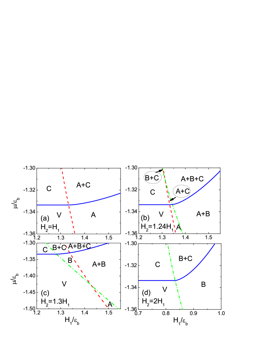
Figure 2: (Color online) The $\mu-H$ phase diagrams at the temperature $T=0.001\varepsilon_{b}$ for (a) pure Zeeman splitting and unequally-spaced Zeeman splitting (b), (c) and (d). $V$ denotes the vacuum phase, $A$ denotes the unpaired fermion phase, $B$ denotes the paired phase and $C$ denotes the trion phase. The phase boundaries are determined by the equation of state (34) which are consistent with the phase diagrams determined via the dressed energy equations, see the description in the text.

with $Q_{1}=\sqrt{\mu+H_{1}}$. This phase diagram is shown in Fig. 2(a).

The phase boundaries for nonlinear Zeeman splitting are obtained in a similar fashion. Indeed we find that all zero temperature phase diagrams are consistent with the $\mu$-$H$ phase diagrams which are directly plotted from the equation of state (34) with the temperature $T=0.001\varepsilon_{b}$, see Fig. 2. For simplicity, we used $A$, $B$ and $C$ to respectively denote the phases of unpaired fermions, pairs and trions. The phases $A$+$B$, $B$+$C$, $A$+$C$ and $A$+$B$+$C$ stand for a mixture of corresponding phases.

The quantum phase segments in an harmonic trapping potential can clearly be discerned from the phase diagrams in Fig. 2. The phase diagram in Fig. 2(a) is for pure Zeeman splitting ($H_{1}=H_{2}$). The multi-critical point in the phase diagram in Fig. 2(a) is located at $\left(\frac{4\varepsilon_{b}}{3},-\frac{4\varepsilon_{b}}{3}\right)$ at $T=0$. It may persist for some non-zero temperatures due to the existence of TLL phases. In an harmonic trapping potential, the mixture of trions and unpaired atoms is at the centre of the trap, whereas the unpaired fermions are at the outer wings when the external field $H>{4\varepsilon_{b}}/{3}$. However, for $H<{4\varepsilon_{b}}/{3}$ almost the whole cloud is the trion phase due to a large binding energy of trions. The mixture of trions and unpaired fermions might lie in a very narrow strip in the trapping centre.

Quantum phase diagrams for unequally-spaced splittings are very intriguing. In the phase diagram Fig. 2(d) the Zeeman splitting parameters are $H_{2}=2H_{1}$. In this case, the pair phase is energetically favoured. From the dressed energy equations we can find that the phase boundaries intersect at $\left(\frac{10\varepsilon_{b}}{12},-\frac{4\varepsilon_{b}}{3}\right)$ at $T=0$. In an harmonic trapping potential, when the external field $H>\frac{10\varepsilon_{b}}{12}$, the centre of trap is a mixture of trions and pairs whereas the outer wings are occupied by pairs. However, for $H<\frac{10\varepsilon_{b}}{12}$, the mixture of trions and paired fermions lie in a narrow strip in the trapping centre. The trions occupy the outer wings.

More subtle quantum phases can be tuned through nonlinear Zeeman splitting, see the phase diagrams in Fig. 2(b) and Fig. 2(c), where the phase diagrams for the chemical potential are shown for the illustrative field values $H_{2}=1.24H_{1}$ and $H_{2}=1.3H_{1}$. The mixture of trions, pairs and unpaired fermions can occur in a certain setting of Zeeman splitting among the three lowest energy levels. The intersection points in the phase diagrams can be easily determined through the equation of state (34) with such settings, but it seems to be more difficult to analytically determine the phase boundaries. These subtle quantum phases can be mapped out through the new scheme proposed in Ho-Zhou from experimental data in trapped 1D Fermi gases. In order to understand the nature of such quantum phases, we turn to the examination of the specific heat in the $T-H$ plane.

IV.2 Specific heat and entropy

The thermodynamics of the system (1) can be analytically calculated through the equation of state (34). All thermodynamic properties then follow analytically through the general thermodynamic relations. According to the formula for the specific heat $c_{v}=\left(\partial^{2}p/\partial T^{2}\right)_{v}$, the phase diagrams as revealed by $c_{v}$ in the $T-H$ plane can be easily explored for fixed total density. Here the specific heat $c_{v}$ is a function of $T$, $\mu$, $H_{1}$ and $H_{2}$. Thus the full $c_{v}$ phase diagram would be four dimensional. In order to observe the signatures of the TLL, we take two-dimensional contour plots for the $c_{v}$ phase diagrams for some illustrative values of Zeeman splitting associated with Fig. 2.

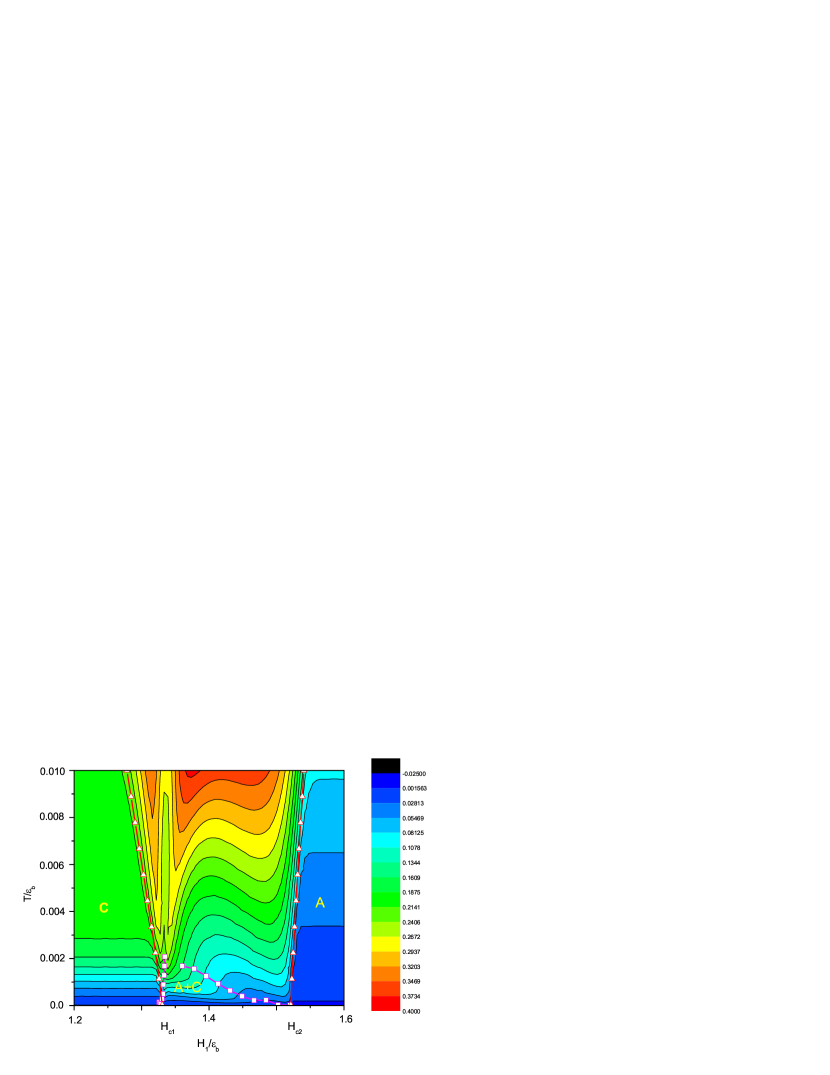
Figure 3: (Color online) The specific heat $c_{v}$ in the $T$-$H_{1}$ plane for pure Zeeman splitting with $H_{1}=H_{2}$ and total density $n$ fixed. An asymmetric two-component TLL remains within a regime below the line of squares between $H_{c1}<H<H_{c2}$. The TLL of spin-neutral trion states and the TLL of unpaired fermionic atoms lie below the left and right line of triangles, respectively.

For pure Zeeman splitting, the gapless phase is described by a two-component TLL phase under a crossover temperature (lines of squares in Fig. 3) which indicates a deviation from the linear temperature-dependent specific heat

$$c_{v}\approx\frac{\pi T}{3\hbar}\left(\frac{1}{v_{1}}+\frac{1}{v_{3}}\right).$$ (39)

The trions and unpaired fermions can form an asymmetric two-component TLL of composite fermions and single atoms for temperatures below the lines of squares. However, the trion phase $C$ and unpaired fermions phase $A$ form two different single-component TLLs which lie below the left and right lines of triangles, respectively. In the single-component TLL phase the other states are exponentially small and thus the system is strongly correlated.

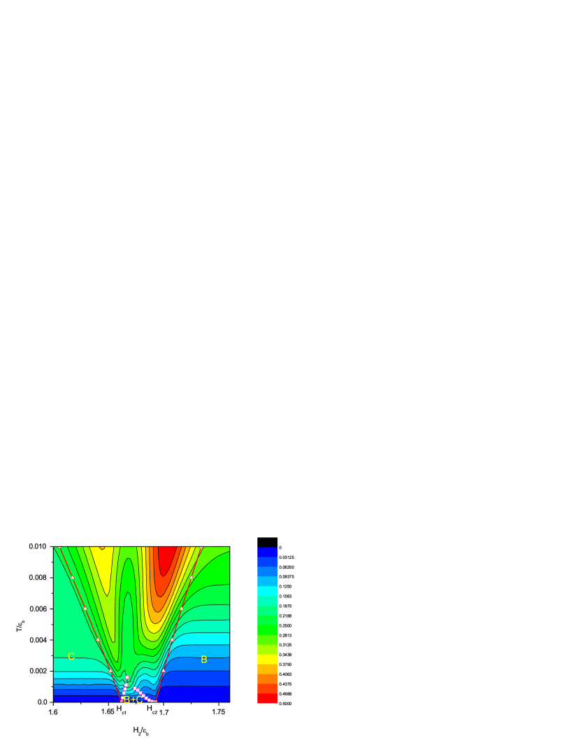
Figure 4: (Color online) The specific heat $c_{v}$ in the $T$-$H_{2}$ plane for $H_{2}=2H_{1}$ with total density $n$ fixed. An asymmetric two-component TLL remains within a regime below the line of squares between $H_{c1}<H<H_{c2}$. The TLL of spin-neutral trions and the TLL of the composite pairs lie below the left and right lines of triangles, respectively.

For unequally spaced Zeeman splitting ($H_{2}=2H_{1}$) the zero temperature phase diagram in Fig. 2(d) may persist for finite $T$ as long as the excitations are close to the Fermi points of each Fermi sea. From the low temperature phase diagram Fig. 4 we see clearly that a two-component TLL of trions and pairs remains in the regime $B+C$. The gapless phase is described by a two-component TLL phase under a crossover temperature delineated by a deviation from the linear temperature-dependent specific heat

$$c_{v}\approx\frac{\pi T}{3\hbar}\left(\frac{1}{v_{2}}+\frac{1}{v_{3}}\right).$$ (40)

In this case a TLL of hard-core bosons of composite fermions lies below the right line of triangles.

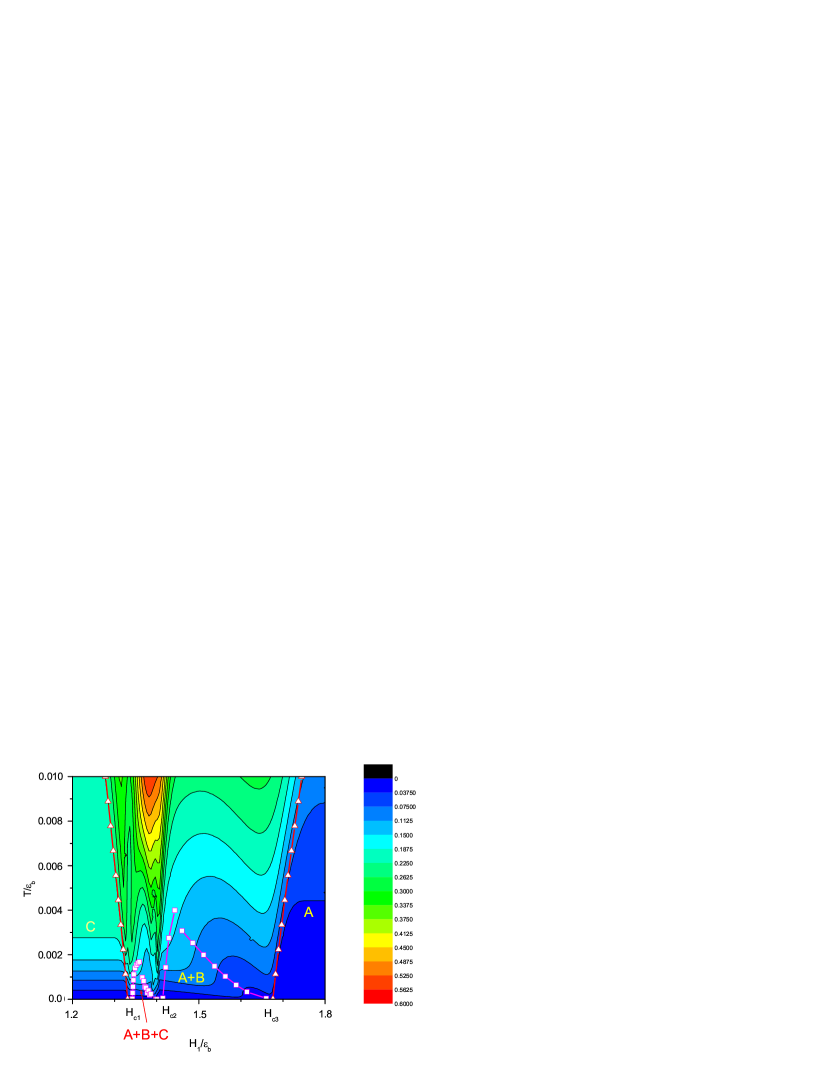
Figure 5: (Color online) The specific heat $c_{v}$ in the $T$-$H_{1}$ plane for $H_{2}=1.2H_{1}$ with total density $n$ fixed. An asymmetric three-component TLL remains within a regime below the line of squares between $H_{c1}<H<H_{c2}$. An asymmetric two-component TLL remains within a regime below the line of pink squares between $H_{c2}<H<H_{c3}$. A TLL of spin-neutral trion states and a TLL of unpaired fermionic atoms lie below the left and right lines of triangles, respectively.

For unequally spaced Zeeman splitting ($H_{2}=1.2H_{1}$) the three-component TLL ($A+B+C$) and two-component TLL ($A+B$) phases may persist within certain regimes in the $T-H$ plane, see the lines of squares in Fig. 5. Beyond the universal crossover temperatures one of the excitations among the states of trions, pairs and unpaired fermions exhibits nonrelativistic dispersion. In the three-component TLL phase, i.e. where trions, pairs and unpaired fermions coexist, the specific heat is given by the linear relation

$$c_{v}\approx\frac{\pi T}{3\hbar}\left(\frac{1}{v_{1}}+\frac{1}{v_{2}}+\frac{1}{v_{3}}\right).$$ (41)

We see clearly that the equation of state (34) provides a precise description of the thermodynamics and critical behaviour of composite fermions.

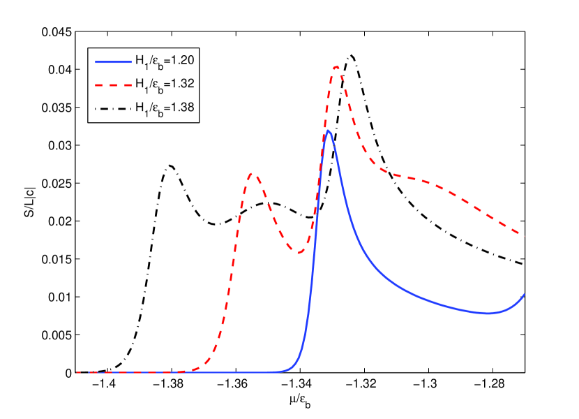
Figure 6: (Color online) Entropy per unit length vs chemical potential with $T/\varepsilon_{b}=0.005$ and $H_{2}=1.3H_{1}$ for different $H_{1}/\varepsilon_{b}$. The entropy exhibits peaks in the phases of higher density of states when the chemical potential passes the critical points, see text.

In Fig. 6, we demonstrate that the entropy exhibits a peak as the driving parameter chemical potential varies across a phase boundary in the $\mu-H$ plane, see Fig. 2(c). The entropy curves are shown in Fig. 6 for the indicative values $H_{1}=1.2\varepsilon_{b},\,1.32\varepsilon_{b}$ and $H_{1}=1.38\varepsilon_{b}$. In this example, the chemical potential thus varies across the different phase boundaries in Fig. 2(c) at which the quantum phase transitions occur. The entropy peaks in Fig. 6 are located in the phases with higher density of states.

V Conclusion

In conclusion, we have studied the thermodynamics of 1D strongly attractive three-component fermions in the presence of nonlinear Zeeman fields via the thermodynamic Bethe ansatz solution. The pressure and free energy have been analytically calculated in terms of the chemical potential $\mu$, temperature $T$ and Zeeman fields $H_{1}$ and $H_{2}$ for a parameter regime $T\ll\varepsilon_{b},\,\varepsilon_{t},\,H_{1},\,H_{2}$ and $\gamma\gg 1$. Here $\varepsilon_{b}$ and $\varepsilon_{t}$ are the binding energies for a bound pair and a trion, respectively. This physical regime covers the presently accessible experimental parameter regime Hulet . The universal thermodynamics of the asymmetric two-component and three-component TLLs has been identified at low temperatures. Beyond a certain crossover temperature, at least one of the underlying dispersion relations for the composite particles is no longer linear and exhibits rich thermal excitations.

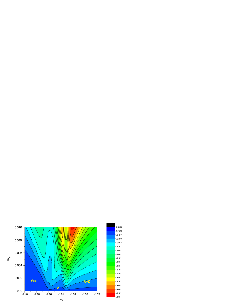
Figure 7: (Color online) Specific heat phase diagram in the $T-\mu$ plane for equally-spaced Zeeman splitting with $H_{1}=1.36\varepsilon_{b}$. The figure shows how the phase diagram extends out from the zero temperature phase diagram.

We have derived the equation of state (34) from which quantum criticality and quantum phase transitions can be mapped out. The equation of state provides the necessary information to describe the quantum regime near quantum critical points. The scaling functions and critical exponents can be obtained from the equation of state following the approach for the two-component model Guan-Ho . With regard to the harmonic trapping of three-component fermions, quantum criticality can be mapped out through the specific heat phase diagram in the $T-\mu$ plane. For example, for equally-spaced Zeeman splitting with $H_{1}=1.36\varepsilon_{b}$, the critical behaviour of the system can be conceived from the specific heat phase diagram in the $T-\mu$ plane, see Fig. 7. Our results thus open the way for further study of quantum criticality in 1D many-body systems via their exact Bethe ansatz solution. In this case for systems of three-component ultracold fermionic atoms.

Appendix A Derivation of the TBA equations

For the 1D three-component fermion system we consider, there are three kinds of states in the system, i.e., unpaired fermions, pairs and trions. In the thermodynamic limit and at zero temperature, there are three kinds of quasimomenta solutions to the BA equations (3). These are real $\left\{k_{i}\right\}$, with $i=1,\ldots,N_{1}$ for the unpaired fermions, complex roots $\left\{k_{l}=\Lambda_{\ell}\pm\frac{1}{2}\mathrm{i}|c|\right\}$ with $\ell=1,\ldots,N_{2}$ for bound pairs and three-body bound states $\left\{k_{m}=\lambda_{m}\pm\mathrm{i}|c|,\,\lambda_{m}\right\}$ with $m=1,\ldots,N_{3}$ for trions.

For finite temperatures, there are also spin strings for spin rapidities $\Lambda$ and $\lambda$, which are characterized by the string-hypothesis

$$\Lambda_{j}^{n,\beta} = \Lambda_{j}^{n}-\frac{1}{2}(n+1-2\beta)\mathrm{i},$$ (42)

$$\lambda_{j}^{n,\beta} = \lambda_{j}^{n}-\frac{1}{2}(n+1-2\beta)\mathrm{i}.$$ (43)

where $n$ is the length of the string, $j$ labels the number of strings of length $n$, and $\Lambda_{j}^{n}$ and $\lambda_{j}^{n}$ are the real parts of each $\Lambda$ and $\lambda$ string. At finite temperatures, there are $N_{1}^{\prime}$ real quasimomenta $k_{j}$, $N_{2}^{\prime}$ real $\Lambda_{j}$ and $N_{3}^{\prime}$ real $\lambda_{j}$. The number of $\Lambda^{(n)}$-strings is $M_{1n}$ and the number of the $\lambda^{(n)}$-strings is $M_{2n}$. These quantum numbers satisfy the conditions

$$M_{1} = N_{2}^{\prime}+2N_{3}^{\prime}+\sum_{n=1}^{\infty}nM_{1n},$$ (44)

$$M_{2} = N_{3}^{\prime}+\sum_{n=1}^{\infty}nM_{2n}.$$ (45)

Substituting these three sets of solutions into the BA equations (3) gives

$$\mathrm{e}^{\mathrm{i}k_{j}L} = \prod_{l=1}^{N_{2}^{\prime}}\frac{k_{j}-\Lambda_{l}+\mathrm{i}|c|/2}{k_{j}-\Lambda_{l}-\mathrm{i}|c|/2}\prod_{l=1}^{N_{3}^{\prime}}\frac{k_{j}-\lambda_{l}+{\mathrm{i}|c|}}{k_{j}-\lambda_{l}-{\mathrm{i}|c|}}\prod_{n=1}^{\infty}\prod_{l=1}^{M_{1n}}\frac{k_{j}-\Lambda_{l}^{n}+\mathrm{i}n|c|/2}{k_{j}-\Lambda_{l}^{n}-\mathrm{i}n|c|/2}$$ (46)

for unpaired fermions and

$$\mathrm{e}^{2\mathrm{i}\Lambda_{j}L} = \prod_{l=1,l\neq j}^{N_{2}^{\prime}}\frac{\Lambda_{j}-\Lambda_{l}+\mathrm{i}|c|}{\Lambda_{j}-\Lambda_{l}-\mathrm{i}|c|}\left(\frac{k_{j}^{(1)}-\Lambda_{j}+\mathrm{i}|c|/2}{k_{j}^{(1)}-\Lambda_{j}-\mathrm{i}|c|/2}\frac{k_{j}^{(2)}-\Lambda_{j}+\mathrm{i}|c|/2}{k_{j}^{(2)}-\Lambda_{j}-\mathrm{i}|c|/2}\right)\prod_{l=1}^{N_{3}^{\prime}}\frac{\Lambda_{j}-\lambda_{l}+3\mathrm{i}|c|/2}{\Lambda_{j}-\lambda_{l}-3\mathrm{i}|c|/2}\frac{\Lambda_{j}-\lambda_{l}+\mathrm{i}|c|/2}{\Lambda_{j}-\lambda_{l}-\mathrm{i}|c|/2}$$ (47)

$$\times\prod_{n=1}^{\infty}\prod_{l=1}^{M_{1n}}\prod_{\beta=1}^{n}\frac{\Lambda_{j}-\Lambda_{l}^{n,\beta}+\mathrm{i}|c|}{\Lambda_{j}-\Lambda_{l}^{n,\beta}-\mathrm{i}|c|}$$

for paired fermions. Notice that Eq. (47) has explicit singularities from the terms in the $()$ bracket. To overcome this, we write the second term of equation of (3) as

$$\prod_{l=1,l\neq j}^{N_{1}^{\prime}}\frac{\Lambda_{j}-k_{l}+\mathrm{i}|c|/2}{\Lambda_{j}-k_{l}-\mathrm{i}|c|/2}\left(\frac{k_{j}^{(1)}-\Lambda_{j}-\mathrm{i}|c|/2}{k_{j}^{(1)}-\Lambda_{j}+\mathrm{i}|c|/2}\frac{k_{j}^{(2)}-\Lambda_{j}-\mathrm{i}|c|/2}{k_{j}^{(2)}-\Lambda_{j}+\mathrm{i}|c|/2}\right)$$

$$\quad=\prod_{n=1}^{\infty}\prod_{m=1}^{M_{1n}}\prod_{\beta=1}^{n}\frac{\Lambda_{j}-\Lambda_{m}^{n,\beta}+\mathrm{i}|c|}{\Lambda_{j}-\Lambda_{m}^{n,\beta}-\mathrm{i}|c|}\prod_{n=1}^{\infty}\prod_{m^{\prime}=1}^{M_{2n}}\prod_{\alpha=1}^{n}\frac{\Lambda_{j}-\lambda_{m^{\prime}}^{n,\alpha}-\mathrm{i}|c|/2}{\Lambda_{j}-\lambda_{m^{\prime}}^{n,\alpha}+\mathrm{i}|c|/2}$$ (48)

which shows the spin flipping of $\Lambda^{n}$-strings. Substituting (48) back to (47) gives the revised form

$$\mathrm{e}^{2\mathrm{i}\Lambda_{j}L} = \prod_{l=1}^{N_{1}^{\prime}}\frac{\Lambda_{j}-k_{l}+\mathrm{i}|c|/2}{\Lambda_{j}-k_{l}-\mathrm{i}|c|/2}\prod_{l=1}^{N_{2}^{\prime}}\frac{\Lambda_{j}-\Lambda_{l}+\mathrm{i}|c|}{\Lambda_{j}-\Lambda_{l}-\mathrm{i}|c|}\prod_{l=1}^{N_{3}^{\prime}}\frac{\Lambda_{j}-\lambda_{l}+3\mathrm{i}|c|/2}{\Lambda_{j}-\lambda_{l}-3\mathrm{i}|c|/2}\frac{\Lambda_{j}-\lambda_{l}+\mathrm{i}|c|/2}{\Lambda_{j}-\lambda_{l}-\mathrm{i}|c|/2}$$ (49)

$$\times\prod_{n=1}^{\infty}\prod_{l=1}^{M_{2n}}\frac{\Lambda_{j}-\lambda_{l}^{n}+\mathrm{i}n|c|/2}{\Lambda_{j}-\lambda_{l}^{n}-\mathrm{i}n|c|/2}$$

for pairs without singularities. Similarly, the equation for trions is

$$\mathrm{e}^{3\mathrm{i}\lambda_{j}L} = \prod_{l=1}^{N_{1}^{\prime}}\frac{\lambda_{j}-k_{l}+\mathrm{i}|c|}{\lambda_{j}-k_{l}-\mathrm{i}|c|}\prod_{l=1}^{N_{2}^{\prime}}\frac{\lambda_{j}-\Lambda_{l}+\mathrm{i}|c|/2}{\lambda_{j}-\Lambda_{l}-\mathrm{i}|c|/2}\frac{\lambda_{j}-\Lambda_{l}+3\mathrm{i}|c|/2}{\lambda_{j}-\Lambda_{l}-3\mathrm{i}|c|/2}$$ (50)

$$\times\prod_{l=1}^{N_{3}^{\prime}}\frac{\lambda_{j}-\lambda_{l}+\mathrm{i}|c|}{\lambda_{j}-\lambda_{l}-\mathrm{i}|c|}\frac{\lambda_{j}-\lambda_{l}+2\mathrm{i}|c|}{\lambda_{j}-\lambda_{l}-2\mathrm{i}|c|}.$$

The BA equations for the spin parts are

$$\prod_{l=1}^{N_{1}^{\prime}}\frac{\Lambda_{j}^{m}-k_{l}-\mathrm{i}m|c|/2}{\Lambda_{j}^{m}-k_{l}+\mathrm{i}m|c|/2} = -\prod_{n=1}^{\infty}\prod_{l=1}^{M_{1n}}\prod_{\beta=1}^{n}\frac{\Lambda_{j}^{m}-\Lambda_{l}^{n}+(m+n+2-2\beta)\mathrm{i}|c|/2}{\Lambda_{j}^{m}-\Lambda_{l}^{n}-(m+n+2-2\beta)\mathrm{i}|c|/2}\,\,\frac{\Lambda_{j}^{m}-\Lambda_{l}^{n}+(m+n-2\beta)\mathrm{i}|c|/2}{\Lambda_{j}^{m}-\Lambda_{l}^{n}-(m+n-2\beta)\mathrm{i}|c|/2}$$ (51)

$$\times\prod_{n=1}^{\infty}\prod_{l=1}^{M_{2n}}\prod_{\beta=1}^{n}\frac{\Lambda_{j}^{m}-\lambda_{l}^{n}+(m+n+1-2\beta)\mathrm{i}|c|/2}{\Lambda_{j}^{m}-\lambda_{l}^{n}-(m+n+1-2\beta)\mathrm{i}|c|/2},$$

$$\prod_{l=1}^{N_{2}^{\prime}}\frac{\lambda_{j}^{m}-\Lambda_{l}+\mathrm{i}m|c|/2}{\lambda_{j}^{m}-\Lambda_{l}-\mathrm{i}m|c|/2} = -\prod_{n=1}^{\infty}\prod_{l=1}^{M_{2n}}\prod_{\beta=1}^{n}\frac{\lambda_{j}^{m}-\lambda_{l}^{n}+(m+n+2-2\beta)\mathrm{i}|c|/2}{\lambda_{j}^{m}-\lambda_{l}^{n}-(m+n+2-2\beta)\mathrm{i}|c|/2}\,\,\frac{\lambda_{j}^{m}-\lambda_{l}^{n}+(m+n-2\beta)\mathrm{i}|c|/2}{\lambda_{j}^{m}-\lambda_{l}^{n}-(m+n-2\beta)\mathrm{i}|c|/2}$$ (52)

$$\times\prod_{n=1}^{\infty}\prod_{l=1}^{M_{1n}}\prod_{\beta=1}^{n}\frac{\lambda_{j}^{m}-\Lambda_{l}^{n}+(m+n+1-2\beta)\mathrm{i}|c|/2}{\lambda_{j}^{m}-\Lambda_{l}^{n}-(m+n+1-2\beta)\mathrm{i}|c|/2}.$$

Defining the function $\theta(x)=2\arctan x$ and taking the logarithm on both sides of the above equations gives

$$k_{j}L = 2\pi I_{j}+\sum_{l=1}^{N_{2}^{\prime}}\theta(\frac{k_{j}-\Lambda_{l}}{|c^{\prime}|})+\sum_{l=1}^{N_{3}^{\prime}}\theta(\frac{k_{j}-\lambda_{l}}{2|c^{\prime}|})+\sum_{n=1}^{\infty}\sum_{l=1}^{M_{1n}}\theta(\frac{k_{j}-\Lambda_{l}^{n}}{n|c^{\prime}|}),$$ (53)

$$2\Lambda_{j}L = 2\pi J_{j}+\sum_{l=1}^{N_{1}^{\prime}}\theta(\frac{\Lambda_{j}-k_{l}}{|c^{\prime}|})+\sum_{l=1}^{N_{2}^{\prime}}\theta(\frac{\Lambda_{j}-\Lambda_{l}}{2|c^{\prime}|})+\sum_{l=1}^{N_{3}^{\prime}}\left[\theta(\frac{\Lambda_{j}-\lambda_{l}}{3|c^{\prime}|})+\theta(\frac{\Lambda_{j}-\lambda_{l}}{|c^{\prime}|})\right]$$ (54)

$$+\sum_{n=1}^{\infty}\sum_{l=1}^{M_{2n}}\theta(\frac{\Lambda_{j}-\lambda_{l}^{n}}{n|c^{\prime}|}),$$

$$3\lambda_{j}L = 2\pi K_{j}+\sum_{l=1}^{N_{1}^{\prime}}\theta(\frac{\lambda_{j}-k_{l}}{2|c^{\prime}|})+\sum_{l=1}^{N_{2}^{\prime}}\left[\theta(\frac{\lambda_{j}-\Lambda_{l}}{|c^{\prime}|})+\theta(\frac{\lambda_{j}-\Lambda_{l}}{3|c^{\prime}|})\right]$$ (55)

$$+\sum_{l=1}^{N_{3}^{\prime}}\left[\theta(\frac{\lambda_{j}-\lambda_{l}}{2|c^{\prime}|})+\theta(\frac{\lambda_{j}-\lambda_{l}}{4|c^{\prime}|})\right],$$

$$\sum_{l=1}^{N_{1}^{\prime}}\theta(\frac{\Lambda_{j}^{m}-k_{l}^{n}}{m|c^{\prime}|}) = 2\pi I_{j}^{(n)}+\sum_{n=1}^{\infty}\sum_{l=1}^{M_{1n}}\Theta_{mn}(\frac{\Lambda_{j}^{m}-\Lambda_{l}^{n}}{|c^{\prime}|})-\sum_{n=1}^{\infty}\sum_{l=1}^{M_{2n}}\Xi_{mn}(\frac{\Lambda_{j}^{m}-\lambda_{l}^{n}}{|c^{\prime}|}),$$ (56)

$$\sum_{l=1}^{N_{2}^{\prime}}\theta(\frac{\lambda_{j}^{m}-\Lambda_{l}^{n}}{m|c^{\prime}|}) = 2\pi J_{j}^{(n)}+\sum_{n=1}^{\infty}\sum_{l=1}^{M_{2n}}\Theta_{mn}(\frac{\lambda_{j}^{m}-\lambda_{l}^{n}}{|c^{\prime}|})-\sum_{n=1}^{\infty}\sum_{l=1}^{M_{1n}}\Xi_{mn}(\frac{\lambda_{j}^{m}-\Lambda_{l}^{n}}{|c^{\prime}|}).$$ (57)

Here $c^{\prime}=c/2$ with $I_{j}$, $J_{j}$, $K_{j}$, $I_{j}^{(n)}$, $J_{j}^{(n)}$ integers or half-odd-integers depending on the quantum numbers.

The functions $\Theta_{mn}$ and $\Xi_{mn}$ are defined by

$$\Theta_{mn} = \left\{\begin{array}[]{l}\theta_{m+n}+2\theta_{m+n-2}+\cdots 2\theta_{|m-n|+2}+\theta_{|m-n|},\quad\mathrm{for}\,\,m\neq n,\\ 2\theta_{2}+2\theta_{4}+\cdots+2\theta_{2n-2}+\theta_{2n},\quad\mathrm{for}\,\,m=n,\end{array}\right.$$ (59)

$$\Xi_{mn} = \left\{\begin{array}[]{l}\theta_{m+n-1}+\theta_{m+n-3}+\cdots\theta_{|m-n|+3}+\theta_{|m-n|+1},\quad\mathrm{for}\,\,m\neq n,\\ \theta_{1}+\theta_{3}+\cdots+\theta_{2n-3}+\theta_{2n-1},\quad\mathrm{for}\,\,m=n.\end{array}\right.$$ (61)

Finally we define the functions

$$h^{\prime}(k) = kL-\sum_{l=1}^{N_{2}^{\prime}}\theta(\frac{k-\Lambda_{l}}{|c^{\prime}|})-\sum_{l=1}^{N_{3}^{\prime}}\theta(\frac{k-\lambda_{l}}{2|c^{\prime}|})-\sum_{n=1}^{\infty}\sum_{l=1}^{M_{1n}}\theta(\frac{k-\Lambda_{l}^{n}}{n|c^{\prime}|}),$$ (62)

$$j^{\prime}(\Lambda) = 2\Lambda L-\sum_{l=1}^{N_{1}^{\prime}}\theta(\frac{\Lambda-k_{l}}{|c^{\prime}|})-\sum_{l=1}^{N_{2}^{\prime}}\theta(\frac{\Lambda-\Lambda_{l}}{2|c^{\prime}|})-\sum_{l=1}^{N_{3}^{\prime}}\left[\theta(\frac{\Lambda-\lambda_{l}}{3|c^{\prime}|})+\theta(\frac{\Lambda-\lambda_{l}}{|c^{\prime}|})\right]-\sum_{n=1}^{\infty}\sum_{l=1}^{M_{2n}}\theta(\frac{\Lambda-\lambda_{l}^{n}}{n|c^{\prime}|}),$$ (63)

$$k^{\prime}\left(\lambda\right) = 3\lambda L-\sum_{l=1}^{N_{1}^{\prime}}\theta(\frac{\lambda-k_{l}}{2|c^{\prime}|})-\sum_{l=1}^{N_{2}^{\prime}}\left[\theta(\frac{\lambda-\Lambda_{l}}{|c^{\prime}|})+\theta(\frac{\lambda-\Lambda_{l}}{3|c^{\prime}|})\right]-\sum_{l=1}^{N_{3}^{\prime}}\left[\theta(\frac{\lambda-\lambda_{l}}{2|c^{\prime}|})+\theta(\frac{\lambda-\lambda_{l}}{4|c^{\prime}|})\right],$$ (64)

and

$$j_{m}(\Lambda^{m}) = \sum_{l=1}^{N_{1}^{\prime}}\theta(\frac{\Lambda^{m}-k_{l}^{n}}{m|c^{\prime}|})-\sum_{n=1}^{\infty}\sum_{l=1}^{M_{1n}}\Theta_{mn}(\frac{\Lambda^{m}-\Lambda_{l}^{n}}{|c^{\prime}|})+\sum_{n=1}^{\infty}\sum_{l=1}^{M_{2n}}\Xi_{mn}(\frac{\Lambda^{m}-\lambda_{l}^{n}}{|c^{\prime}|}),$$ (65)

$$k_{m}(\lambda^{m}) = \sum_{l=1}^{N_{1}^{\prime}}\theta(\frac{\lambda^{m}-\Lambda_{l}^{n}}{m|c^{\prime}|})-\sum_{n=1}^{\infty}\sum_{l=1}^{M_{2n}}\Theta_{mn}(\frac{\lambda^{m}-\lambda_{l}^{n}}{|c^{\prime}|})+\sum_{n=1}^{\infty}\sum_{l=1}^{M_{1n}}\Xi_{mn}(\frac{\lambda^{m}-\Lambda_{l}^{n}}{|c^{\prime}|}).$$ (66)

In the thermodynamic limit, we then define

$$\frac{dh^{\prime}(k)}{dk} = 2\pi(\rho_{1}(k)+\rho_{1}^{h}(k)),$$ (67)

$$\frac{dj^{\prime}(\Lambda)}{d\Lambda} = 2\pi(\rho_{2}(\Lambda)+\rho_{2}^{h}(\Lambda)),$$ (68)

$$\frac{dk^{\prime}\left(\lambda\right)}{dk} = 2\pi(\rho_{3}\left(\lambda\right)+\rho_{3}^{h}\left(\lambda\right)),$$ (69)

$$\frac{dj_{n}(\Lambda^{n})}{d\Lambda^{n}} = 2\pi(\sigma_{n}(\Lambda^{n})+\sigma_{n}^{h}(\Lambda^{n})),$$ (70)

$$\frac{dk_{n}(\lambda^{n})}{d\lambda^{n}} = 2\pi(\tau_{n}(\lambda^{n})+\tau_{n}^{h}(\lambda^{n})).$$ (71)

where $\rho_{i}$ and $\rho_{i}^{h}$ for $i=1,2,3$ are particle and hole densities in $k$-space, and $\sigma_{n}$, $\sigma_{n}^{h}$ and $\tau_{n}$, $\tau_{n}^{h}$ are particle densities and hole densities for strings with length $n$ in $\Lambda$-space and $\lambda$-space.

Thus we have the integral equations

$$\frac{1}{2\pi} = \rho_{1}+\rho_{1}^{h}+a_{1}*\rho_{2}+a_{2}*\rho_{3}+\sum_{n}a_{n}*\sigma_{n},$$ (72)

$$\frac{1}{\pi} = \rho_{2}+\rho_{2}^{h}+a_{1}*\rho_{1}+a_{2}*\rho_{2}+\,(a_{1}+a_{3})*\rho_{3}+\sum_{n}a_{n}*\tau_{n},$$ (73)

$$\frac{3}{2\pi} = \rho_{3}+\rho_{3}^{h}+a_{2}*\rho_{1}+(a_{1}+a_{3})*\rho_{2}+\,(a_{2}+a_{4})*\rho_{3},$$ (74)

for the particle and hole densities and

$$a_{n}*\rho_{1} = \sigma_{n}+\sigma_{n}^{h}+\sum_{m}T_{mn}*\sigma_{m}-\,\sum_{m}S_{mn}*\tau_{m},$$ (75)

$$a_{n}*\rho_{2} = \tau_{n}+\tau_{n}^{h}+\sum_{m}T_{mn}*\tau_{m}-\,\sum_{m}S_{mn}*\sigma_{m}.$$ (76)

where the functions $T_{mn}$ and $S_{mn}$ are defined as

$$T_{mn} = \left\{\begin{array}[]{l}a_{m+n}+2a_{m+n-2}+\cdots 2a_{|m-n|+2}+a_{|m-n|},\quad\mathrm{for}\,\,m\neq n,\\ 2a_{2}+2a_{4}+\cdots+2a_{2n-2}+a_{2n},\quad\mathrm{for}\,\,m=n,\end{array}\right.$$ (78)

and

$$S_{mn} = \left\{\begin{array}[]{l}a_{m+n-1}+a_{m+n-3}+\cdots a_{|m-n|+3}+a_{|m-n|+1},\quad\mathrm{for}\,\,m\neq n,\\ a_{1}+a_{3}+\cdots+a_{2n-3}+a_{2n-1},\quad\mathrm{for}\,\,m=n.\end{array}\right.$$ (80)

The energy per unit length can now be written as

$$E/L = \int k^{2}\rho_{1}(k)dk+\int(2k^{2}-\frac{c^{2}}{2})\rho_{2}(k)dk+\int(3k^{2}-2c^{2})\rho_{3}(k)dk.$$ (81)

The total particle number and magnetic numbers are

$$N/L = \int(\rho_{1}(k)+2\rho_{2}(k)+3\rho_{3}(k))dk,$$ (82)

$$M_{1}/L = \int\rho_{2}(k)dk+2\int\rho_{3}(k)dk+\,\sum_{n}n\int\sigma_{n}(\Lambda^{n})d\Lambda^{n},$$ (83)

$$M_{2}/L = \int\rho_{3}(k)dk+\sum_{n}n\int\tau_{n}(\lambda^{n})d\lambda^{n}.$$ (84)

The entropy per unit length is

$$S/L = \int((\rho_{1}+\rho_{1}^{h})\ln(\rho_{1}+\rho_{1}^{h})-\rho_{1}\ln\rho_{1}-\rho_{1}^{h}\ln\rho_{1}^{h})dk+\int((\rho_{2}+\rho_{2}^{h})\ln(\rho_{2}+\rho_{2}^{h})-\rho_{2}\ln\rho_{2}-\rho_{2}^{h}\ln\rho_{2}^{h})dk$$ (85)

$$+\int((\rho_{3}+\rho_{3}^{h})\ln(\rho_{3}+\rho_{3}^{h})-\rho_{3}\ln\rho_{3}-\rho_{3}^{h}\ln\rho_{3}^{h})dk$$

$$+\sum_{n}\int((\sigma_{n}+\sigma_{n}^{h})\ln(\sigma_{n}+\sigma_{n}^{h})-\sigma_{n}\ln\rho_{1}\sigma_{n}-\,\sigma_{n}^{h}\ln\sigma_{n}^{h})dk$$

$$+\sum_{n}\int((\sigma_{n}+\sigma_{n}^{h})\ln(\sigma_{n}+\sigma_{n}^{h})-\sigma_{n}\ln\rho_{1}\sigma_{n}-\,\sigma_{n}^{h}\ln\sigma_{n}^{h})dk,$$

where $\ln n!\approx n\ln n$ has been used.

The Gibbs energy (4) per unit length is

$$G/L = \int k^{2}\rho_{1}dk+\int(2k^{2}-\frac{c^{2}}{2})\rho_{2}dk+\int(3k^{2}-2c^{2})\rho_{3}dk-\mu\int(\rho_{1}+2\rho_{2}+3\rho_{3})dk$$ (86)

$$-H_{1}\int(\rho_{1}-2\sum_{n}n\sigma_{n}+\sum_{n}n\tau_{n})dk-H_{2}\int(\rho_{2}+\sum_{n}n\sigma_{n}-2\sum_{n}n\tau_{n})dk-TS.$$

Finally, the TBA equations follow by taking the variation of equation (86) and setting it equal to zero, i.e. $\delta G/L=0$. In this way

$$\ln\eta_{1} = (k^{2}-\mu-H_{1})/{T}\,+a_{1}\ast\ln(1+\eta_{2}^{-1})+\,a_{2}\ast\ln(1+\eta_{3}^{-1})-\,\sum_{n=1}^{\infty}a_{n}\ast\ln(1+\xi_{n}^{-1}),$$ (87)

$$\ln\eta_{2} = ({2\Lambda^{2}-\frac{1}{2}{c^{2}}-2\mu-H_{2}})/{T}+a_{1}\ast\ln(1+\eta_{1}^{-1})+\,a_{2}\ast\ln(1+\eta_{2}^{-1})+(a_{1}+a_{3})\ast\ln(1+\eta_{3}^{-1})$$ (88)

$$-\,\sum_{n=1}^{\infty}a_{n}\ast\ln(1+\zeta_{n}^{-1}),$$

$$\ln\eta_{3} = \frac{3\lambda^{2}-2{c^{2}}-3\mu}{T}+a_{2}\ast\ln(1+\eta_{1}^{-1})+\,(a_{1}+a_{3})\ast\ln(1+\eta_{2}^{-1})+\,(a_{2}+a_{4})\ast\ln(1+\eta_{3}^{-1})$$ (89)

and

$$\ln\xi_{n} = {n(2H_{1}-H_{2})}/{T}\,+a_{n}\ast\ln(1+e^{-{\varepsilon_{1}}/{T}})+\,\sum_{m}T_{mn}\ast\ln(1+\xi_{m}^{-1})-\,\sum_{m}S_{mn}\ast\ln(1+\zeta_{m}^{-1}),$$ (90)

$$\ln\zeta_{n} = {n(2H_{2}-H_{1})}/{T}\,+a_{n}\ast\ln(1+e^{-{\varepsilon_{2}}/{T}})+\,\sum_{m}T_{mn}\ast\ln(1+\zeta_{m}^{-1})-\,\sum_{m}S_{mn}\ast\ln(1+\xi_{m}^{-1}),$$ (91)

in which we define $\eta_{i}=\rho_{i}^{h}/\rho_{i}$ ($i=1,2,3$), $\xi_{n}=\sigma_{n}^{h}/\sigma_{n}$ and $\zeta_{n}=\tau_{n}^{h}/\tau_{n}$. The TBA equations (87)-(91) can be written in the form (5) with $\varepsilon_{i}=T\ln\eta_{a}$ ($a=1,2,3$).

Appendix B Details of the Sommerfeld expansion

In this Appendix, we show that accurate expressions for $\mu$ and $p$ can be obtained by iteration after Sommerfeld expansion. We first use equation (11) to rewrite the pressure (13) in the form

$$p^{(1)}\approx\frac{2}{3\pi}(\mu^{(1)})^{{3}/{2}}\left(1+\frac{\pi^{2}}{8}\left(\frac{T}{A^{(1)}}\right)^{2}\right)\left(1-\frac{2p^{(2)}}{|c|\mu^{(1)}}-\frac{2p^{(3)}}{3|c|\mu^{(1)}}\right)^{{3}/{2}},$$ (92)

$$p^{(2)}\approx\frac{2\sqrt{2}}{3\pi}(2\mu^{(2)})^{{3}/{2}}\left(1+\frac{\pi^{2}}{8}\left(\frac{T}{A^{(2)}}\right)^{2}\right)\left(1-\frac{2p^{(1)}}{|c|\mu^{(2)}}-\frac{p^{(2)}}{2|c|\mu^{(2)}}-\frac{8p^{(3)}}{9|c|\mu^{(2)}}\right)^{{3}/{2}},$$ (93)

$$p^{(3)}\approx\frac{2\sqrt{3}}{3\pi}(3\mu^{(3)})^{{3}/{2}}\left(1+\frac{\pi^{2}}{8}\left(\frac{T}{A^{(3)}}\right)^{2}\right)\left(1-\frac{2p^{(1)}}{3|c|\mu^{(3)}}-\frac{8p^{(2)}}{9|c|\mu^{(3)}}-\frac{p^{(3)}}{3|c|\mu^{(3)}}\right)^{{3}/{2}}.$$ (94)

We can extract explicit analytic results appropriate for the strong coupling regime $|c|\gg 1$ from these equations by iteration and neglecting higher order terms. Making use of equations (14) and $n=n_{1}+2n_{2}+3n_{3}$, we obtain expressions for $n$, $n_{1}$, $n_{2}$ and $n_{3}$. After a lengthy calculation, we then obtain $\mu^{(1)}$, $\mu^{(2)}$ and $\mu^{(3)}$ in terms of $n_{1}$, $n_{2}$ and $n_{3}$, namely

$$\mu^{(1)} \approx n_{1}^{2}{\pi^{2}}\left[1+\frac{16}{3|c|\pi}\frac{(\mu^{(2)})^{{3}/{2}}}{\mu^{(1)}}\left(1+\frac{\pi^{2}}{8}\left(\frac{T}{A^{(2)}}\right)^{2}\right)+\frac{4}{|c|\pi}\frac{(\mu^{(3)})^{{3}/{2}}}{\mu^{(1)}}\left(1+\frac{\pi^{2}}{8}\left(\frac{T}{A^{(3)}}\right)^{2}\right)\right.$$ (95)

$$\left.+\frac{16}{|c|}\frac{\sqrt{\mu^{(2)}}}{\pi}\left(1-\frac{\pi^{2}}{24}\left(\frac{T}{A^{(2)}}\right)^{2}\right)+\frac{12}{|c|}\frac{\sqrt{\mu^{(3)}}}{\pi}\left(1-\frac{\pi^{2}}{24}\left(\frac{T}{A^{(3)}}\right)^{2}\right)\right]\left(1+\frac{\pi^{2}}{12}\left(\frac{T}{A^{(1)}}\right)^{2}\right),$$

$$\mu^{(2)} \approx \frac{n_{2}^{2}}{4}{\pi^{2}}\left[1+\frac{4}{3|c|\pi}\frac{(\mu^{(1)})^{{3}/{2}}}{\mu^{(2)}}\left(1+\frac{\pi^{2}}{8}\left(\frac{T}{A^{(1)}}\right)^{2}\right)+\frac{16}{3|c|\pi}\sqrt{\mu^{(2)}}\right.$$ (96)

$$\left.+\frac{16}{3|c|\pi}\frac{(\mu^{(3)})^{{3}/{2}}}{\mu^{(2)}}\left(1+\frac{\pi^{2}}{8}\left(\frac{T}{A^{(3)}}\right)^{2}\right)+\frac{4}{|c|}\frac{\sqrt{\mu^{(1)}}}{\pi}\left(1-\frac{\pi^{2}}{24}\left(\frac{T}{A^{(1)}}\right)^{2}\right)\right.$$

$$\left.+\frac{16}{|c|}\frac{\sqrt{\mu^{(3)}}}{\pi}\left(1-\frac{\pi^{2}}{24}\left(\frac{T}{A^{(3)}}\right)^{2}\right)\right]\left(1+\frac{\pi^{2}}{12}\left(\frac{T}{A^{(2)}}\right)^{2}\right),$$

$$\mu^{(3)} \approx \frac{n_{3}^{2}}{9}{\pi^{2}}\left[1+\frac{4}{9|c|\pi}\frac{(\mu^{(1)})^{{3}/{2}}}{\mu^{(3)}}\left(1+\frac{\pi^{2}}{8}\left(\frac{T}{A^{(1)}}\right)^{2}\right)+\frac{64}{27|c|\pi}\frac{(\mu^{(2)})^{{3}/{2}}}{\mu^{(3)}}\left(1+\frac{\pi^{2}}{8}\left(\frac{T}{A^{(2)}}\right)^{2}\right)\right.$$ (97)

$$\left.+\frac{8}{|c|\pi}\sqrt{\mu^{(3)}}+\frac{4}{3|c|}\frac{\sqrt{\mu^{(1)}}}{\pi}\left(1-\frac{\pi^{2}}{24}\left(\frac{T}{A^{(1)}}\right)^{2}\right)+\frac{64}{9|c|}\frac{\sqrt{\mu^{(2)}}}{\pi}\left(1-\frac{\pi^{2}}{24}\left(\frac{T}{A^{(2)}}\right)^{2}\right)\right]$$

$$\times\left(1+\frac{\pi^{2}}{12}\left(\frac{T}{A^{(2)}}\right)^{2}\right).$$

Substituting (95)-(97) and (13) into (11) and keeping terms to order ${1}/{|c|}$, gives the explicit form for $A^{(a)}$

$$A^{(1)} \approx n_{1}^{2}{\pi^{2}}\left(1+\frac{8}{|c|}n_{2}+\frac{4}{|c|}n_{3}\right),$$ (98)

$$A^{(2)} \approx \frac{n_{2}^{2}}{2}{\pi^{2}}\left(1+\frac{4}{|c|}n_{1}+\frac{2}{|c|}n_{2}+\frac{16}{3|c|}n_{3}\right),$$ (99)

$$A^{(3)} \approx \frac{n_{3}^{2}}{3}{\pi^{2}}\left(1+\frac{4}{3|c|}n_{1}+\frac{32}{9|c|}n_{2}+\frac{2}{|c|}n_{3}\right).$$ (100)

The explicit form for $\mu^{(a)}$ without $A^{(a)}$ terms can also be obtained as

$$\mu^{(1)} \approx n_{1}^{2}{\pi^{2}}\left\{\frac{\pi^{2}}{6}\left(\frac{T}{n_{1}^{2}{\pi^{2}}}\right)^{2}+\frac{2}{3|c|}\frac{n_{2}^{3}}{n_{1}^{2}}\left[1+\frac{\pi^{2}}{4}\left(\frac{T}{\frac{n_{2}^{2}}{2}\pi^{2}}\right)^{2}\right]+\frac{4}{27|c|}\frac{n_{3}^{3}}{n_{1}^{2}}\left[1+\frac{\pi^{2}}{4}\left(\frac{T}{\frac{n_{3}^{2}}{3}\pi^{2}}\right)^{2}\right]\right.$$ (101)

$$+\left.\left[1+\frac{8}{|c|}n_{2}+\frac{4}{|c|}n_{3}\right]\left[1-\frac{\pi^{2}}{12}\left(\frac{T}{n_{1}^{2}{\pi^{2}}}\right)^{2}\right]\right\},$$

$$\mu^{(2)} \approx \frac{n_{2}^{2}}{4}\pi^{2}\left\{\frac{\pi^{2}}{6}\left(\frac{T}{\frac{n_{2}^{2}}{2}}\right)^{2}+\frac{16}{3|c|}\frac{n_{1}^{3}}{n_{2}^{2}}\left[1+\frac{\pi^{2}}{4}\left(\frac{T}{n_{1}^{2}{\pi^{2}}}\right)^{2}\right]+\frac{64}{81|c|}\frac{n_{3}^{3}}{n_{2}^{2}}\left[1+\frac{\pi^{2}}{4}\left(\frac{T}{\frac{n_{3}^{2}}{3}}\right)^{2}\right]+\frac{8}{3|c|}n_{2}\right.$$ (102)

$$+\left.\left[1+\frac{4}{|c|}n_{1}+\frac{16}{3|c|}n_{3}\right]\left[1-\frac{\pi^{2}}{12}\left(\frac{T}{\frac{n_{2}^{2}}{2}}\right)^{2}\right]\right\},$$

$$\mu^{(3)} \approx \frac{n_{3}^{2}}{9}\pi^{2}\left\{\frac{\pi^{2}}{6}\left(\frac{T}{\frac{n_{3}^{2}}{3}{\pi^{2}}}\right)^{2}+\frac{4}{|c|}\frac{n_{1}^{3}}{n_{3}^{2}}\left[1+\frac{\pi^{2}}{4}\left(\frac{T}{n_{1}^{2}{\pi^{2}}}\right)^{2}\right]+\frac{8}{3|c|}\frac{n_{2}^{3}}{n_{3}^{2}}\left[1+\frac{\pi^{2}}{4}\left(\frac{T}{\frac{n_{2}^{2}}{2}}\right)^{2}\right]+\frac{8}{3|c|}n_{3}\right.$$ (103)

$$+\left.\left[1+\frac{4}{3|c|}n_{1}+\frac{32}{9|c|}n_{2}\right]\left[1+\frac{\pi^{2}}{12}\left(\frac{T}{\frac{n_{3}^{2}}{3}{\pi^{2}}}\right)^{2}\right]\right\}.$$

Substitute all of these equations back into (92)-(94) and neglecting higher order terms gives the pressure $p$ given in (17).

Appendix C Dressed energy equations at low temperature

For the strongly attractive regime, the TBA equations (5) can be expanded as

$$\varepsilon_{1}(k) \approx k^{2}-\mu-H_{1}+\frac{2}{|c|}p^{(2)}+\frac{2}{3|c|}p^{(3)}-\,T\sum_{n}\int a_{n}(\frac{2k}{c}-k^{\prime})\ln(1+\xi^{-1})dk^{\prime},$$ (104)

$$\varepsilon_{2}(k) \approx 2k^{2}-2\mu-\frac{c^{2}}{2}-H_{2}+\frac{4}{|c|}p^{(1)}+\frac{1}{|c|}p^{(2)}+\frac{16}{9|c|}p^{(3)}-\,T\sum_{n}\int a_{n}(\frac{2k}{c}-k^{\prime})\ln(1+\zeta^{-1})dk^{\prime},$$ (105)

$$\varepsilon_{3}(k) \approx 3k^{2}-3\mu-2c^{2}+\frac{2}{|c|}p^{(1)}+\frac{8}{3|c|}p^{(2)}+\frac{1}{|c|}p^{(3)},$$ (106)

with

$$\ln\xi_{n}(\Lambda) = \frac{n(2H_{1}-H_{2})}{T}+\frac{2\pi J_{1}}{T}a_{n}(\Lambda)+\,\sum_{m}T_{mn}\ast\ln(1+\xi_{m}^{-1})-\,\sum_{m}S_{mn}\ast\ln(1+\zeta_{m}^{-1}),$$ (107)

$$\ln\zeta_{n}(\lambda) = \frac{n(2H_{2}-H_{1})}{T}+\frac{2\pi J_{2}}{T}a_{n}(\Lambda)+\,\sum_{m}T_{mn}\ast\ln(1+\zeta_{m}^{-1})-\sum_{m}S_{mn}\ast\ln(1+\xi_{m}^{-1}).$$ (108)

Here $J_{1}=2p_{1}/|c|$, $J_{2}=p_{2}/|c|$ and the function $a_{n}(k)$ has the new form

$$a_{n}(k)=\frac{1}{2\pi}\frac{2n}{k^{2}+n^{2}}.$$ (109)

Compared with equation (10), the last terms of (104) and (105) are string terms for spin waves of unpaired fermions and pairs, respectively. From $\ln\xi$ and $\ln\zeta$, we have

$$\xi_{n}(\Lambda) \approx \mathrm{e}^{{n(2H_{1}-H_{2})}/{T}}\mathrm{e}^{{2\pi J_{1}a_{1}(\Lambda)}/{T}}\,\mathrm{e}^{\sum_{m}T_{mn}\ast\xi_{m}^{-1}}\mathrm{e}^{-\sum_{m}S_{mn}\ast\zeta_{m}^{-1}},$$ (110)

$$\zeta_{n}(\lambda) \approx \mathrm{e}^{{n(2H_{2}-H_{1})}/{T}}\mathrm{e}^{{2\pi J_{2}a_{2}(\lambda)}/{T}}\,\mathrm{e}^{\sum_{m}T_{mn}\ast\zeta_{m}^{-1}}\,\mathrm{e}^{-\sum_{m}S_{mn}\ast\xi_{m}^{-1}}.$$ (111)

Neglecting higher order correction terms we finally arrive at the dressed energy equations (32). The pressure can readily be written in terms of the polylogarithm function using (32) and (12).