The size of the longest filament in the Luminous Red Galaxy distribution

Abstract

Filaments are one of the most prominent features visible in the galaxy distribution. Considering the Luminous Red Galaxies (LRGs) in the Sloan Digital Sky Survey Data Release Seven (SDSS DR7), we have analyzed the filamentarity in $11$ nearly two dimensional (2D) sections through a volume limited subsample of this data. The galaxy distribution, we find, has excess filamentarity in comparison to a random distribution of points. We use a statistical technique “Shuffle” to determine $L_{\rm MAX}$, the largest length-scale at which we have statistically significant filaments. We find that $L_{\rm MAX}$ varies in the range $100-130\,h^{-1}{\rm Mpc}$ across the $11$ slices, with a mean value $L_{\rm MAX}=110\pm 12\,h^{-1}{\rm Mpc}$. Longer filaments, though possibly present in our data, are not statistically significant and are the outcome of chance alignments.

1 Introduction

One of the main goals of redshift surveys is to study the galaxy distribution. Various redshift surveys (e.g. CfA, Geller & Huchra 1989; LCRS, Shectman et al. 1996; 2dFGRS, Colles et al. 2001 and SDSS, Stoughton et al. 2002) all show that galaxies are distributed in an interconnected network of clusters, sheets and filaments encircling nearly empty voids. This complex network is often referred to as the “Cosmic Web”. Quantifying the cosmic web and understanding it’s origin is a challenging problem in cosmology.

The analysis of filamentary patterns in the galaxy distribution has a long history dating back to a few papers in the late-seventies and mid-eighties by Joeveer et al. (1978), Einasto et al. (1980), Zel’dovich , Einasto & Shandarin (1982), Shandarin & Zeldovich (1983) and Einasto et al. (1984). Filaments are the most striking visible patterns seen in the galaxy distribution (e.g. Geller & Huchra 1989, Shectman et al. 1996, Shandarin & Yess 1998, Bharadwaj et al. 2000, Müller et al. 2000, Basilakos, Plionis, & Rowan-Robinson 2001, Doroshkevich et al. 2004, Pimbblet, Drinkwater & Hawkrigg 2004, Pandey & Bharadwaj 2005).

Are the filaments statistically significant? This is a question that naturally arises when we embark on studying the filaments in the galaxy distribution. The possibility that the observed filaments are not genuine feature of the galaxy distribution and could arise out of chance alignments requires us to establish the statistical significance of the filaments.

The SDSS (York et al., 2000) is currently the largest galaxy redshift survey. Pandey & Bharadwaj (2005) (hereafter Paper I) have analyzed the filamentarity in the equatorial strips of this survey. These strips are nearly two dimensional (2D). They have projected the data onto a plane and analyzed the resulting 2D galaxy distribution. They find evidence for connectivity and filamentarity in excess of that of a random point distribution, indicating the existence of an interconnected network of filaments. The filaments are statistically significant upto a length scales of $80\,h^{-1}{\rm Mpc}$ and not beyond (Pandey & Bharadwaj, 2005). All the structures spanning length-scales greater than this length scale are the result of chance alignments. These results are consistent with the earlier findings from Las Campanas Redshift Survey (LCRS) where the filamentarity was found to be statistically significant on scales up to $70-80\,h^{-1}\,{\rm Mpc}$ in the $-3^{\circ}$ slice and $50-70\,h^{-1}\,{\rm Mpc}$ in the other 5 slices (Bharadwaj et al., 2004). The average filamentarity of the galaxy distribution was shown to depend on various physical galaxy properties such as the luminosity, colour, morphology and star formation rate (Pandey & Bharadwaj, 2006, 2008). Recently Pandey (2010) has studied if the statistically significant length scale of filaments depends on different galaxy properties and finds that it does not depend on the galaxy luminosity, colour and morphology. Analysis with mock galaxy samples from N-body simulations indicates that the length scale upto which filaments are statistically significant is also nearly independent of bias and weakly depends on the number density and size of the galaxy samples.

The measurement of the length scale upto which the filaments are statistically significant could be limited by the size of the survey, and it is possible that this has been underestimated in earlier studies with the LCRS and the SDSS MAIN galaxy sample. This issue can be addressed repeating the analysis with a bigger galaxy survey. Given a magnitude limit, Luminous Red Galaxies (LRGs) can be observed to greater distances as compared to normal $L_{\star}$ galaxies. Further their stable colors make them relatively easy to pick out from the rest of the galaxies using the SDSS multi-band photometry. The LRG sample extends to a much deeper region of the Universe as compared to the SDSS MAIN galaxy sample. The very large region covered by the SDSS LRG sample provides us the ideal opportunity to investigate the size of the longest filaments present in the Universe.

In this work we measure the largest lengthscale at which we have statistically significant filaments in the distribution of LRGs in the SDSS DR7. We discuss the data and method of analysis in Section 2, and the results and conclusions are presented in Section 3.

Throughout our work, we have used the flat $\Lambda$CDM cosmology with $\Omega_{m}=0.3,\;\Omega_{\Lambda}=0.7\mbox{ and }h=1$.

2 Data and Method of Analysis

2.1 SDSS data

The Sloan Digital Sky Survey (SDSS) (York et al., 2000) is a wide-field imaging and spectroscopic survey of the sky using a dedicated 2.5 m telescope (Gunn et al., 2006) with $3^{\circ}$ field of view at Apache Point Observatory in southern New Mexico. The SDSS has imaged the sky in 5 passbands, $u,\;g,\;r,\;i$ and $z$ covering $10^{4}$ square degrees and has so far made 7 data releases to the community. The SDSS galaxy sample can be roughly divided into two (i) the MAIN galaxy sample and (ii) the Luminous Red Galaxy (LRG) sample. For our work, we have used the spectroscopic sample of LRGs derived from the Data Release 7 of SDSS-II (Abazajian et al., 2009).

SDSS targets those galaxies for spectroscopy which have $r$ magnitude brighter than 17.77 ($r<17.77$). To select LRGs, additional galaxies are targeted using color-magnitude cuts in $g,\;r$ and $i$ which extends the magnitude limit for LRGs to $r<19.5$. The prominent feature for an early-type galaxy is the $4000\,A^{\circ}$ break in its SED. For $z\lesssim 0.4$ this feature lies in the $g$ passband while it shifts to the $r$ band for higher redshifts. Hence selection of LRGs involves different selection criteria below and above $z\lesssim 0.4$, the details of which are described in Eisenstein et.al. (2001) (hereafter E01).

The criteria for lower redshifts are collectively called Cut-I (eq. (4-9) in E01) while those for the higher redshifts are called Cut-II (eq. (9-13) in E01), with Cut-I accounting for $\approx 80\%$ of the targeted LRGs. A galaxy that passes either of these cuts is flagged for spectroscopy by the SDSS pipeline as TARGET_GALAXY_RED while a galaxy that passes only Cut II is flagged as TARGET_GALAXY_RED_II. Hence, while selecting the LRGs we require that the TARGET_GALAXY_RED and TARGET_GALAXY_RED_II flags both be set.

We obtain the $g$-band absolute magnitude from the $r$ band apparent magnitude accounting for the k-correction and passive evolution. We use the prescription for $K+e$ correction from the Table 1 in E01 (non-star forming model). The cuts defined above are designed to produce an approximately volume limited sample of LRGs upto $z\approx 0.4$. The comoving number density of LRGs falls sharply beyond $z\approx 0.4$. It is obviously necessary to include LRGs that come from the MAIN sample for $z\lesssim 0.3$. But E01 issue a strong advisory against selecting LRGs with $z\lesssim 0.15$ for a volume limited sample as the luminosity threshold is not preserved for low redshifts. We have restricted our LRG sample to the redshift range $0.16<z<0.38$ and $g$-band absolute magnitude range $-23<M_{g}<-21$. Figure 1 shows the LRG number density as a function of the radial distance $r$ for the $r$ range that we have used in our analysis. We see that the LRG density has a maximum variation of $\sim 30\%$ around the mean density. An earlier study (Pandey & Bharadwaj, 2006) indicates that a density variation of this order is not expected to produce a statistically significant effect on the average filamentarity. The earlier study also indicates that the length scale upto which the filaments are statistically significant has a very weak dependence on the density.

Figure 2 shows the geometry of the sky coverage of the region that we have analyzed in survey coordinates $\lambda$ and $\eta$ (Stoughton et al., 2002). For our analysis we have extracted $11$ strips that are described in the Table 1. Each strip spans $100^{\circ}$ in $\lambda$ ($-50<\lambda<50$) and $3^{\circ}$ in $\eta$ ($\eta$ ranges are shown in Table 1), and radially extends from $462h^{-1}{\rm Mpc}$ to $1037h^{-1}{\rm Mpc}$. Adjacent strips are separated by $3^{\circ}$. The physical thickness of each strip increases with radial distance. We have extracted strips of uniform thickness $24h^{-1}{\rm Mpc}$ which corresponds to $3^{\circ}$ at a radial distance of $462h^{-1}{\rm Mpc}$. The volume outside these uniform thickness strips was discarded from our analysis.

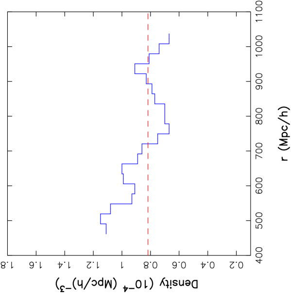
Figure 1: The density of LRGs as a function of radial distance $r$. The density has been computed using shells of uniform thickness $28.75h^{-1}{\rm Mpc}$ in the radial direction. The dashed line shows the mean density of our LRG sample.

Figure 2: The geometry of the 11 LRG strips extracted from SDSS DR7 plotted in survey coordinates.

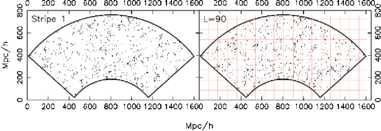
Figure 3: The left panel shows the projected 2D galaxy distribution in one of the LRG strips. The right panel shows a shuffled realization generated from the same data using $L=90h^{-1}{\rm Mpc}$. The corresponding $90h^{-1}{\rm Mpc}\,\times\,90h^{-1}{\rm Mpc}$ grid is overlaid. The blocks defined by this grid were randomly interchanged with a rotation. Only blocks that are entirely within the survey area are used in this process.

Table 1: Details of the LRG samples extracted from SDSS DR7

Strip name	$\eta_{min}$	$\eta_{max}$	$n$
S1	-33.5	-30.5	1211
S2	-27.5	-24.5	1332
S3	-21.5	-18.5	1477
S4	-15.5	-12.5	1513
S5	-9.50	-6.50	1590
S6	-3.50	-0.500	1568
S7	2.50	5.50	1677
S8	8.50	11.5	1601
S9	14.5	17.5	1422
S10	20.5	23.5	1169
S11	26.5	29.5	1356

2.2 Method of Analysis

The strips that we have analyzed extend $575\,h^{-1}{\rm Mpc}$ in the radial direction and $\sim 800\,h^{-1}{\rm Mpc}$ (or more) in the transverse direction, while the thickness is only $24\,h^{-1}{\rm Mpc}$. These strips can be treated as nearly two dimensional which makes the analysis relatively simpler. The strips were all collapsed along the thickness (the smallest dimension) to produce a 2D galaxy distributions (Figure 3). We use the 2D “Shapefinder” statistic (Bharadwaj et al., 2000) to quantify the filamentarity of the patterns in the resulting galaxy distribution. A detailed discussion is presented in Pandey & Bharadwaj (2006), and we present only the salient features here. The reader is referred to Sahni, Sathyaprakash,& Shandarin (1998) for a discussion of Shapefinders in three dimensions (3D).

The galaxy distribution was embedded in a 2D mesh $760\,h^{-1}{\rm Mpc}\times 1608\,h^{-1}{\rm Mpc}$ with cell size $2\,h^{-1}{\rm Mpc}\times 2\,h^{-1}{\rm Mpc}$. The entire galaxy distribution was represented as a set of 1s and 0s on the mesh. Cells containing a galaxy were assigned a value $1$, and the empty cells were assigned a value $0$. Note the difference in grid size from the Pandey & Bharadwaj (2005) where a $1\,{\rm Mpc\,}h^{-1}\times 1\,{\rm Mpc\,}h^{-1}$ cell was used. This takes into account the fact that our LRG strips have projected galaxy number density $\simeq 1.9\times 10^{-3}({\rm Mpc\,}h^{-1})^{-2}$which is considerably smaller than $\simeq 9\times 10^{-3}({\rm Mpc\,}h^{-1})^{-2}$ in the samples analyzed in Paper I.

We use the ‘Friends-of-Friend’ (FOF) algorithm to identify connected regions of filled cells which we refer to as clusters. The filamentarity of each cluster is quantified using the Shapefinder ${\cal F}$ which defined as

$${\cal F}=\frac{(P^{2}-16S)}{(P-4l)^{2}}$$ (1)

where $P$ and $S$ are respectively the perimeter and the area of the cluster, and $l$ is the grid spacing. The Shapefinder ${\cal F}$ has values $0$ and $1$ for a square and filament respectively, and it assumes intermediate values as a square is deformed to a filament. We use the average filamentarity

$$F_{2}={\sum_{i}{\cal S}_{i}^{2}{\cal F}_{i}\over\sum_{i}{\cal S}_{i}^{2}}\,.$$ (2)

to asses the overall filamentarity of the clusters in the galaxy distribution.

The distribution of 1s corresponding to the galaxies is sparse. Only $\lesssim 1\%$ of the cells contain galaxies and there are very few filled cells which are interconnected. As a consequence FOF fails to identify the large coherent structures which correspond to filaments in the galaxy distribution. We overcome this by successively coarse-graining the galaxy distribution. This is achieved by gradually making the filled cells fatter. In each iteration of coarse-graining all the empty cells adjacent to a filled cell (i.e. cells at the 4 sides and 4 corners of a filled cell) are assigned a value $1$ . This causes clusters to grow, first because of the growth of individual filled cells, and then by the merger of adjacent clusters as they overlap. Coherent structures extending across progressively larger length-scales are identified in consecutive iterations of coarse-graining. So as not to restrict our analysis to an arbitrarily chosen level of coarse-graining, we study the average filamentarity after each iteration of coarse-graining. The filling factor $FF$ quantifies the fraction of cells that are filled and its value increases from $\sim 0.01$ and approaches $1$ as the coarse-graining proceeds. We study the average filamentarity $F_{2}$ as a function of the filling factor $FF$ (Figure 4) as a quantitative measure of the filamentarity at different levels of coarse-graining. The values of $FF$ corresponding to a particular level of coarse-graining shows a slight variation from strip to strip. In order to combine and compare the results from different strips, for each strip we have interpolated $F_{2}$ to $7$ values of $FF$ at a uniform spacing of $0.1$ over the interval $0.05$ to $0.65$. Coarse-graining beyond $FF\sim 0.65$ washes away the filaments and hence we do not include this range for our analysis. For comparison we also consider a random reference sample generated by randomly distributing points over a 2D region with exactly the same geometry and number density as the projected LRG samples. We find that the filamentarity of the LRG data is in excess of that of the random samples (Figure 4). While this is reassuring that we are studying a genuine signal, it should be interpreted with some caution. It is possible that the enhanced filamentarity observed in the actual data would also arise if the observed two-point clustering were incorporated in the random samples even in the absence of higher order clustering. In this paper we use a statistical technique called Shuffle, which does not rely on externally generated random samples, to establish the length-scale upto which the observed filamentarity is statistically significant. Shuffle was first introduced and applied by Bhavsar & Ling (1988). Subsequent work (Bharadwaj et al., 2004; Pandey & Bharadwaj, 2005; Pandey, 2010) has extended this and applied it to the LCRS, the SDSS Main galaxy sample and N-body simulations.

A grid with squares blocks of side $L$ is superposed on the original data slice (Figure 3). The blocks which lie entirely within the survey area are then randomly interchanged, with rotation, repeatedly to form a new shuffled data. The shuffling process eliminates coherent features in the original data on length-scales larger than $L$, keeping structures at length-scales below $L$ intact. All the structures spanning length-scales greater than $L$ that exist in the shuffled slices are the result of chance alignments. At a fixed value of $L$, the average filamentarity in the original sample will be larger than in the shuffled data only if the actual data has more filaments spanning length-scales larger than $L$, than that expected from chance alignments. The largest value of $L$, $L_{\rm MAX}$, for which the average filamentarity of the shuffled slices is less than the average filamentarity of the actual data gives us the largest length-scale at which the filamentarity is statistically significant. Filaments spanning length-scales larger than $L_{\rm MAX}$ arise purely from chance alignments.

For each value of $L$ we have generated $24$ different realization of the shuffled slices. To ensure that the edges of the blocks which are shuffled around do not cut the actual filamentary pattern at exactly the same place in all the realizations of the shuffled data, we have randomly shifted the origin of the grid used to define the blocks. The values of FF and $F_{2}$ in the 24 realizations differ from one another and from the actual data at the same stage of coarse-graining. So as to be able to quantitatively compare the shuffled realizations with the actual data, results from the shuffled data were interpolated in the same way as actual data. The mean $\bar{F_{2}}[{\rm Shuffled}]$ and the variance $(\Delta F_{2}[{\rm Shuffled}])^{2}$ of the average filamentarity was determined for the shuffled data at each value of FF using the $24$ realizations. The difference between the filamentarity of the actual data and its shuffled counterparts was quantified using the reduced $\chi^{2}$ per degree of freedom

$$\frac{\chi^{2}}{\nu}=\frac{1}{N_{p}}\sum_{a=1}^{N_{p}}\frac{(F_{2}[{\rm Actual}]-\bar{F_{2}}[{\rm Shuffled}]))_{a}^{2}}{(\Delta F_{2}[{\rm Shuffled}])_{a}^{2}}$$ (3)

where the sum is over different values of the filling factor FF.

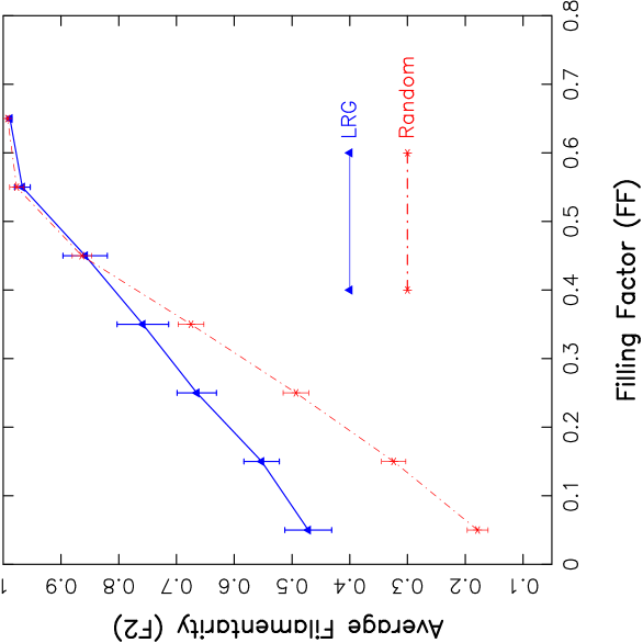
Figure 4: The Average Filamentarity ($F_{2}$) as a function of the Filling Factor ($FF$). The mean and $1-\sigma$ errors from $11$ strips are shown for both the LRG strips and the corresponding random realisations.

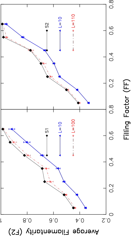
Figure 5: The Average Filamentarity ($F_{2}$) as a function of the Filling Factor ($FF$) for strips S1 (left) and S2 (right) of the LRG data. The effect of shuffling with $L=10h^{-1}\,{\rm Mpc}$ is shown for both strips. The other value of $L$ corresponds to $L_{\rm MAX}$ which is different for the two strips. Notice that at $L_{\rm MAX}$ the actual data points lie just outside the $1-\sigma$ error-bars of the shuffled data. For the shuffled data we have shown the mean and $1-\sigma$ errors from $24$ independent realizations of the shuffling process.

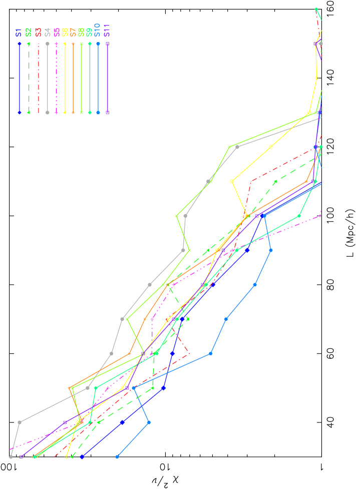
Figure 6: This shows $\chi^{2}/\nu$ as a function of $L$ for all the $11$ LRG strips that we have analyzed.

3 Results and Conclusions

Figure 5 shows the effect of shuffling the LRG data for $2$ of the $11$ strips. We see that shuffling with $L=10\,h^{-1}{\rm Mpc}$ causes $F_{2}$ to drop considerably relative to the unshuffled data. It is thus established that the filaments are statistically significant at this length-scale. We have varied $L$ in steps of $10\,h^{-1}{\rm Mpc}$ form $L=10\,h^{-1}{\rm Mpc}$ to $160\,h^{-1}{\rm Mpc}$. We find that the difference between the actual and the shuffled data is reduced (ie. $F_{2}$ increases) as $L$ is increased. The filamentarity in the actual data and its shuffled counterparts are consistent for $L=160\,h^{-1}{\rm Mpc}$ indicating that at this length-scale the filaments are not statistically significant but are the outcome of chance alignments. All the $11$ LRG strips analyzed here show a similar behaviour.

We consider $\chi^{2}/\nu$ to quantify the difference between the filamentarity of the actual data and its shuffled counterparts. This difference is not considered to be statistically significant if $\chi^{2}/\nu\sim 1$. For all the $11$ strips, Figure 6 shows $\chi^{2}/\nu$ for different values of $L$. The value of $\chi^{2}/\nu$ falls with increasing $L$. We define $L_{\rm MAX}$ as the largest $L$ value for which there is a statistically significant difference caused by shuffling. Increasing $L$ beyond $L_{\rm MAX}$ causes $\chi^{2}/\nu$ to fall such that $\chi^{2}/\nu\sim 1$. Considering the particular strip shown in the left panel of Figure 5, we see that $L_{MAX}=100\,h^{-1}{\rm Mpc}$ i.e. there is a statistically significant difference between the average filamentarity of the actual data and its shuffled counterparts for $L\leq L_{\rm MAX}=100\,h^{-1}{\rm Mpc}$ but not beyond. The value of $L_{MAX}$ varies in the range $100-130$ across the $11$ strips that we have analyzed. We have averaged the values of $L_{MAX}$ measured in the $11$ different strips to find that $L_{\rm MAX}=110\pm 12\,h^{-1}{\rm Mpc}$. This is the largest length-scale at which we have statistically significant filaments in our LRG strips. Filaments longer than this, though possibly present in the data, are the outcome of chance alignments.

The value of $L_{\rm MAX}$ estimated using the LRGs is somewhat larger than the values in the range $70-80\,h^{-1}{\rm Mpc}$ obtained in earlier studies using the LCRS (Bharadwaj et al., 2004) and the SDSS MAIN galaxy sample (Pandey & Bharadwaj, 2005). This is possibly a consequence of the fact that LRG strips cover a much larger area as compared to the ones analyzed earlier. For example, the SDSS strips analyzed in Pandey & Bharadwaj (2005) have an extent of $336$ and $373\,h^{-1}{\rm Mpc}$ in the radial and transverse directions respectively, in comparison to $575$ and $800h^{-1}{\rm Mpc}$ for the strips analyzed here. The larger area ensures a better mixing of the blocks in the shuffling process. This is particularly important at large $L$ where we had very few blocks in the smaller strips that had been analyzed earlier. The larger area also ensures that the present estimate of $L_{\rm MAX}$ is less likely to be influenced by local effects, and hence is more representative of the global value.

Finally we note that tests with controlled mock samples (Pandey, 2010) show that the 2D analysis adopted here tends to shorten the length of 3D filaments. Further, 3D sheets will appear as filaments in 2D. It is thus necessary to be cautious in interpreting the consequence of our finding in terms of the full 3D galaxy distribution. It is reasonable to interpret $L_{\rm MAX}=110\pm 12\,h^{-1}{\rm Mpc}$ as an order of magnitude estimate of the largest length-scale at which we have statistically significant structures (sheets and filaments) in the 3D LRG distribution.

4 Acknowledgment

Computations were carried out at the IUCAA HPC facility. GK acknowledges support through a postdoctoral position under the DST-Swarnajayanti fellowship grant of TS. GK acknowledges James Annis for his help in understanding the LRG data.

The SDSS DR7 data was downloaded from the SDSS skyserver http://cas.sdss.org/dr7/en/.

Funding for the creation and distribution of the SDSS Archive has been provided by the Alfred P. Sloan Foundation, the Participating Institutions, the National Aeronautics and Space Administration, the National Science Foundation, the U.S. Department of Energy, the Japanese Monbukagakusho, and the Max Planck Society. The SDSS Web site is http://www.sdss.org/.

The SDSS is managed by the Astrophysical Research Consortium (ARC) for the Participating Institutions. The Participating Institutions are The University of Chicago, Fermilab, the Institute for Advanced Study, the Japan Participation Group, The Johns Hopkins University, the Korean Scientist Group, Los Alamos National Laboratory, the Max-Planck-Institute for Astronomy (MPIA), the Max-Planck-Institute for Astrophysics (MPA), New Mexico State University, University of Pittsburgh, Princeton University, the United States Naval Observatory, and the University of Washington.

References

- Abazajian et al. (2009) Abazajian, K. N., et al. 2009, ApJS, 182, 543
- Basilakos, Plionis, & Rowan-Robinson (2001) Basilakos, S., Plionis, M., & Rowan-Robinson, M. 2001, MNRAS, 323, 47
- Bharadwaj et al. (2000) Bharadwaj, S., Sahni, V., Sathyaprakash, B. S., Shandarin, S. F., & Yess, C. 2000, ApJ, 528, 21
- Bharadwaj et al. (2004) Bharadwaj, S., Bhavsar, S. P., & Sheth, J. V. 2004, ApJ, 606, 25
- Bhavsar & Ling (1988) Bhavsar, S. P. & Ling, E. N. 1988, ApJL, 331, L63
- Colles et al. (2001) Colles, M. et al.(for 2dFGRS team) 2001,MNRAS,328,1039
- Doroshkevich et al. (2004) Doroshkevich, A., Tucker, D. L., Allam, S.,& Way, M. J. 2004, A&A, 418,7
- Einasto et al. (1980) Einasto, J., Joeveer, M., & Saar, E. 1980, MNRAS, 193, 353
- Einasto et al. (1984) Einasto, J., Klypin, A. A., Saar, E., & Shandarin, S. F. 1984, MNRAS, 206, 529
- Eisenstein et.al. (2001) Eisenstein, D. J., et al., 2001, AJ, 122, 2267
- Geller & Huchra (1989) Geller, M.J. & Huchra, J.P.1989, Science, 246, 897
- Gunn et al. (2006) Gunn, J. E., et al. 2006, AJ, 131, 2332
- Hogg et al. (2005) Hogg, D. W., Eisenstein, D. J., Blanton, M. R., Bahcall, N. A., Brinkmann, J., Gunn, J. E., & Schneider, D. P. 2005, ApJ, 624, 54
- Joeveer et al. (1978) Joeveer, M., Einasto, J., & Tago, E. 1978, MNRAS, 185, 357
- Müller et al. (2000) Müller, V., Arbabi-Bidgoli, S., Einasto, J., & Tucker, D. 2000, MNRAS, 318, 280
- Pandey & Bharadwaj (2005) Pandey, B. & Bharadwaj, S. 2005, MNRAS, 357, 1068
- Pandey & Bharadwaj (2006) Pandey, B. & Bharadwaj, S. 2006, MNRAS, 372, 827
- Pandey & Bharadwaj (2007) Pandey, B., & Bharadwaj, S. 2007, MNRAS, 377, L15
- Pandey & Bharadwaj (2008) Pandey, B., & Bharadwaj, S. 2008, MNRAS, 387, 767
- Pandey (2010) Pandey, B. 2010, MNRAS, 401, 2687
- Pimbblet, Drinkwater & Hawkrigg (2004) Pimbblet, K. A., Drinkwater, M. J., & Hawkrigg, M. C. 2004, MNRAS, 354, L61
- Sahni, Sathyaprakash,& Shandarin (1998) Sahni, V., Sathyaprakash, B. S., & Shandarin, S. F. 1998, ApJL, 495, L5
- Shandarin & Zeldovich (1983) Shandarin, S. F. & Zeldovich, I. B. 1983, Comments on Astrophysics, 10, 33
- Shandarin & Yess (1998) Shandarin, S. F. & Yess, C. 1998, ApJ, 505, 12
- Shectman et al. (1996) Shectman, S. A.,Landy, S. D., Oemler, A., Tucker, D. L., Lin, H., Kirshner, R. P., & Schechter, P. L. 1996, ApJ, 470, 172
- Stoughton et al. (2002) Stoughton, C., et al. 2002, AJ, 123, 485
- York et al. (2000) York, D. G., et al. 2000, AJ, 120, 1579
- Zel’dovich , Einasto & Shandarin (1982) Zel’dovich, I. B., Einasto, J., & Shandarin, S. F. 1982, Nature, 300, 407