The Nernst effect from fluctuating pairs in the pseudogap phase

Abstract

The observation of a large Nernst signal in cuprates above the superconducting transition temperature has attracted much attention. A potential explanation is that it originates from superconducting fluctuations. Although the Nernst signal is indeed consistent with gaussian fluctuations for overdoped cuprates, gaussian theory fails to describe the temperature dependence seen for underdoped cuprates. Here, we consider the vertex correction to gaussian theory resulting from the pseudogap. This yields a Nernst signal in good agreement with the data.

For most of the doping phase diagram, high temperature superconductivity in the cuprates emerges from a normal state where an energy gap is already present.Timusk The origin of this ‘pseudogap’ is the subject of much debate.Kallin One of the most interesting observations in the pseudogap phase is the existence of a large Nernst signal.Xu ; Wang The Nernst effect is the generation of a transverse electric field by a thermal gradient in the presence of a magnetic field perpendicular to both. Since vortices carry entropy, it is natural to attribute such a large Nernst signal in proximity to the superconducting transition temperature $T_{c}$ to vortex-like excitations.Xu ; Wang Moreover, invoking vortices is consistent with the Nernst signal smoothly going through $T_{c}$. On the other hand, it is not clear whether vortices give an adequate description of the physics of fluctuating superconductors except very near $T_{c}$.Uss04 The free vortex density above the Kosterlitz-Thouless temperature increases exponentially with temperature, a dependence which is inconsistent with the near power-law decrease of the actual Nernst signal above $T_{c}$. Moreover, the recent observation of a negative Nernst signal for underdoped YBa₂Cu₃O_6+y has further complicated the story.Louis This negative signal has been argued to be a consequence of density wave reconstruction of the Fermi surface.

Here, we take the point of view that the dominant contribution to the Nernst signal in the pseudogap phase is indeed due to fluctuating pairs. This is supported by the close correspondence of the Nernst signal with the fluctuational diagmagnetism.Li10 On the other hand, we note that although existing theories based on Ginzburg-Landau or diagrammatic approaches Dorsey ; Uss02 ; Serbyn give a good description of the Nernst data for overdoped cuprates, they do less well for underdoped cuprates. We attribute this to the presence of the pseudogap.

As discussed in Ref. Serbyn, , it is the direct contribution from fluctuating pairs - the Aslamazov-Larkin (AL) contribution AL - which governs the Nernst signal over a wide range of temperatures above $T_{c}$, so we focus on that. The AL contribution to the Nernst coefficient is obtained from the electric current-heat current Kubo response kernel $\Lambda_{xy}$.Uss02 ; Serbyn The latter can be expressed in terms of corresponding electric and heat vertex blocks (triangular graphs) connected by interaction lines (pair fluctuations). The vertex block can be expressed as $\mathrm{Tr}\{\gamma^{(e,h)}\mathbf{B}\}$ with $\mathbf{B}=\left\langle\mathbf{v}GGG\right\rangle$ where $\mathbf{v}$ is the Fermi velocity, and $\langle...\rangle$ indicates disorder averaging. The factor $\gamma$ differentiates the electric vertex ($\gamma^{(e)}=e$) from the heat vertex $\gamma^{(h)}$, which we will discuss below. Disorder averaging in $\mathbf{B}$ leads to the presence of two Cooperons and the renormalization of the free electron Greens function $G$ by impurity scattering. In order to account for the pseudogap, we replace this $G$ which was previously used to compute this block by the broadened BCS Greens function

$$G(k,\varepsilon)=-\frac{i\bar{\varepsilon}+\xi_{k}}{\bar{\varepsilon}^{2}+\xi_{k}^{2}+\Delta_{k}^{2}}$$ (1)

as this gives a good description of photoemission data in the pseudogap phase.Norm98 ; Tallon ; Norm07 In Eq. (1), $\Delta_{k}$ is the momentum dependent pseudogap and $\bar{\varepsilon}=\varepsilon+\Gamma\,\mathrm{sgn}(\varepsilon)$ with $\Gamma$ the scattering rate. By recomputing the electromagnetic vertex block with this $G$, we find that $\mathbf{B}$ is renormalized by a function of $\Delta/\Gamma$ where $\Delta$ is the maximum value of the pseudogap. Assuming a $T$ independent $\Delta$ and $\Gamma\sim T$ as observed in photoemission,Norm98 ; Kanigel this renormalization results in a fluctuation Nernst signal which drops off considerably faster with temperature than the gaussian result. As we show, this gives a good description of the Nernst data for underdoped cuprates.

We assume the standard expression for the pair propagator whose retarded component has the form book

$$L_{R}(q,\omega)=-\frac{1}{N_{0}}\frac{1}{\epsilon-i\pi\omega/8T+\eta q^{2}}$$ (2)

Here, $\epsilon=\ln(T/T_{c})$, $N_{0}$ is the density of states, and $\eta=\pi D/8T$ where $D$ is the diffusion constant. The Nernst coefficient can be expressed in terms of the electrical ($\hat{\sigma}$) and thermoelectric $(\hat{\alpha})$ tensors as $\nu=(\alpha_{xy}\sigma_{xx}-\alpha_{xx}\sigma_{xy})/H(\sigma_{xx}^{2}+\sigma_{xy}^{2})\approx\alpha_{xy}/H\sigma_{xx}$. The second (approximate) expression, which becomes exact if particle-hole symmetry is present, gives a good approximation to $\nu$ for the case of superconducting fluctuations since $\alpha_{xy}\gg\alpha_{xx}$ and $\sigma_{xx}\gg\sigma_{xy}$ (see Ref. book, for a corresponding discussion). The transverse thermoelectric coefficient, $\alpha_{xy}=\bar{\alpha}_{xy}+cM_{z}/T$, consists of two independent contributions: the response of the total current to the applied electric and magnetic fields ($\bar{\alpha}_{xy}$), and the magnetization currents as derived from the equilibrium magnetization $M_{z}$. Like Refs. Uss02, ; Serbyn, , we focus on the first contribution

$$\bar{\alpha}_{xy}=\frac{H}{cT}\lim_{Q,\Omega\to 0}\frac{1}{Q\Omega}\mathrm{Re}[\Lambda_{xy}^{R}(Q,\Omega)]$$ (3)

assuming here weak field limit. The electric current-heat current Kubo response kernel

$$\hskip-7.11317pt\Lambda_{xy}(Q,i\Omega_{m})=-4e^{2}T\sum_{q,\omega_{n}}B_{x}(q)B^{2}_{y}(q)(i\omega_{n}+i\Omega_{m}/2)$$

$$\left[L(q-Q_{x},i\omega_{n})L(q,i\omega_{n})L(q,i\omega_{n}+i\Omega_{m})\right.$$

$$+\left.L(q,i\omega_{n})L(q,i\omega_{n}+i\Omega_{m})L(q+Q_{x},i\omega_{n}+i\Omega_{m})\right]$$ (4)

is written in Matsubara representation, where we have assumed that the heat vertex is $-i\omega_{n}/(2e)$ times the electric vertex.heat In Eq. (The Nernst effect from fluctuating pairs in the pseudogap phase), the Greens function block $B$, whose renormalization is the subject of this paper, is assumed to be independent of frequency. This approximation is formally exact in the immediate vicinity of the transition temperature. Nevertheless, a rigorous extension of this approximation to a wider range of temperatures above $T_{c}$ demonstrates that the Ginzburg-Landau result, $\nu^{AL}\sim\left(T-T_{c}\right)^{-1}$, remains valid even far from $T_{c}$ if one substitutes $T-T_{c}$ by the more general expression $T\ln(T/T_{c})$. We note that in the gaussian approximation book

$$B_{i}^{G}(q)=-2N_{0}\eta q_{i}$$ (5)

For the following linear response calculation we expand the propagators in Eq. (The Nernst effect from fluctuating pairs in the pseudogap phase) to the leading order in $Q$, namely $L(q\pm Q_{x},i\omega_{n})\to\pm Q\partial_{q_{x}}L(q,i\omega_{n})$, and noting that

$$\frac{\partial L(q,i\omega_{n})}{\partial q_{x}}=-B_{x}^{G}(q)L^{2}(q,i\omega_{n})$$ (6)

we thus find from Eq. (The Nernst effect from fluctuating pairs in the pseudogap phase)

$$\hskip-14.22636pt\Lambda_{xy}(Q,i\Omega_{m})=$$ (7)

$$\hskip-14.22636pt-4e^{2}QT\sum_{q,\omega_{n}}B_{x}(q)B_{x}^{G}(q)B_{y}^{2}(q)(i\omega_{n}+i\Omega_{m}/2)$$

$$\hskip-14.22636pt\big{[}L^{3}(q,i\omega_{n})L(q,i\omega_{n}+i\Omega_{m})-L(q,i\omega_{n})L^{3}(q,i\omega_{n}+i\Omega_{m})\big{]}$$

Performing the summation over the Matsubara frequency $\omega_{n}$ by using contour integration, $T\sum_{\omega_{n}}f(i\omega_{n})=\frac{1}{4\pi i}\oint_{C}d\omega\coth\frac{\omega}{2T}f(\omega)$ with two branch-cuts at $\mathrm{Im}(\omega)=0$ and $\mathrm{Im}(\omega)=-\Omega_{m}$, followed by an analytic continuation $\Omega_{m}\rightarrow-i\Omega$, and keeping only the linear in $\Omega$ contribution from $\Lambda_{xy}^{R}(Q,\Omega)$, one finds for the transverse thermoelectric coefficient

$$\hskip-21.33955pt\bar{\alpha}_{xy}^{AL}=\frac{4e^{2}H}{\pi cT}\sum_{q}B_{x}^{G}(q)B_{x}(q)B_{y}^{2}(q)\int_{-\infty}^{+\infty}d\omega\coth\frac{\omega}{2T}$$

$$\hskip-21.33955pt\left\{\![\mathrm{Re}L_{R}(q,\omega)]^{3}\mathrm{Im}L_{R}(q,\omega)\!+\!\mathrm{Re}L_{R}(q,\omega)[\mathrm{Im}L_{R}(q,\omega)]^{3}\right\}$$ (8)

After the remaining momentum and energy integrations, we get the result (restoring $\hbar$)

$$\bar{\alpha}_{xy}^{AL}=\frac{e}{2\pi\hbar}\frac{\xi^{2}_{GL}}{\ell_{H}^{2}}(B/B^{G})^{3}$$ (9)

where $\ell_{H}=\sqrt{\hbar c/eH}$ is the magnetic length and $\xi^{2}_{GL}=\eta/\ln(T/T_{c})$. For $B=B^{G}$, this is the well known expression for the Nernst effect from fluctuating pairs.Uss02 ; Serbyn

At this point, all we have done is to rederive the gaussian expression. The reason we have done this is to demonstrate explicitly where the $B_{i}$ current vertices enter. We now discuss the renormalization of $B_{i}$ due to the pseudogap. The expression for the vertex is AL

$$B_{i}(q,\omega,\Omega)=T\sum_{p,\varepsilon}v_{i}(p)G(p,\varepsilon)G(p,\varepsilon+\Omega)G(q-p,\omega-\varepsilon)$$ (10)

where $\varepsilon$ is the fermionic loop frequency, $\omega$ the bosonic frequency that enters the fluctuation propagator, $\Omega$ the external field frequency (set to zero for the dc response), and $G$ the Greens function.cooperons We will now recalculate $B_{i}$ using the pseudogap Greens function. Substituting Eq. (1) in the previous equation, taking the dc limit, and approximating $G(q-p,\omega-\varepsilon)\approx G(q-p,-\varepsilon)$ we obtain

$$B_{i}(q)\simeq-T\sum_{p,\varepsilon}v_{i}\left(\frac{i\bar{\varepsilon}+\xi_{p}}{\bar{\varepsilon}^{2}+\xi_{p}^{2}+\Delta_{p}^{2}}\right)^{2}\frac{-i\bar{\varepsilon}+\xi_{q-p}}{\bar{\varepsilon}^{2}+\xi_{q-p}^{2}+\Delta_{p}^{2}}$$ (11)

Keeping the term to linear order in $q$,

$$B_{i}(q) \simeq \frac{1}{2}Tv_{F}^{2}q_{i}\sum_{p,\varepsilon}\left(\frac{i\bar{\varepsilon}+\xi_{p}}{\bar{\varepsilon}^{2}+\xi_{p}^{2}+\Delta_{p}^{2}}\right)^{2}$$ (12)

$$\left[\frac{1}{\bar{\varepsilon}^{2}+\xi_{p}^{2}+\Delta_{p}^{2}}-\frac{2\xi_{p}(-i\bar{\varepsilon}+\xi_{p})}{(\bar{\varepsilon}^{2}+\xi_{p}^{2}+\Delta_{p}^{2})^{2}}\right]$$

Converting the $p$ sum to an integral, we have

$$B_{i}(q) \simeq \frac{1}{2}N_{0}Tv_{F}^{2}q_{i}\sum_{\varepsilon}\int\frac{d\vartheta}{2\pi}\int_{-\infty}^{+\infty}d\xi$$ (13)

$$\left[\frac{\xi^{2}-\bar{\varepsilon}^{2}}{(\bar{\varepsilon}^{2}+\xi^{2}+\Delta_{\vartheta}^{2})^{3}}-\frac{2\xi^{2}(\xi^{2}+\bar{\varepsilon}^{2})}{(\bar{\varepsilon}^{2}+\xi^{2}+\Delta_{\vartheta}^{2})^{4}}\right]$$

where $\Delta_{\vartheta}=\Delta\cos 2\vartheta$ (i.e., we assume a d-wave pseudogap). Next we perform the $\xi$ integral by introducing $\xi=\mu x$ with $\mu=\sqrt{\bar{\varepsilon}^{2}+\Delta_{\vartheta}^{2}}$

$$B_{i}(q) \simeq \frac{1}{4\pi}N_{0}Tv_{F}^{2}q_{i}\sum_{\varepsilon}\int\frac{d\vartheta}{(\bar{\varepsilon}^{2}+\Delta_{\vartheta}^{2})^{5/2}}$$ (14)

$$\int_{-\infty}^{+\infty}\!\!dx\left[\frac{\mu^{2}x^{2}-\bar{\varepsilon}^{2}}{(1+x^{2})^{3}}-\frac{2x^{2}(\mu^{2}x^{2}+\bar{\varepsilon}^{2})}{(1+x^{2})^{4}}\right]$$

The $x$ integral is trivial, and we find

$$B_{i}(q)\simeq-\frac{1}{8}N_{0}Tv_{F}^{2}q_{i}\sum_{\varepsilon}\int\frac{\bar{\varepsilon}^{2}d\vartheta}{(\bar{\varepsilon}^{2}+\Delta_{\vartheta}^{2})^{5/2}}$$ (15)

The angular integral is easily performed, leading to

$$B_{i}(q) = -\frac{1}{3}N_{0}Tv_{F}^{2}q_{i}\sum_{n=0}^{\infty}\frac{1}{\bar{\varepsilon}^{2}}\frac{1}{(\bar{\varepsilon}^{2}+\Delta^{2})^{3/2}}$$ (16)

$$\left[(4\bar{\varepsilon}^{2}+2\Delta^{2})E(\lambda)-\bar{\varepsilon}^{2}K(\lambda)\right]$$

where $\lambda=\Delta/\sqrt{\bar{\varepsilon}^{2}+\Delta^{2}}$ and $K$ and $E$ are elliptic functions. As the sum converges at $n\gtrsim\Delta/T$, one can approximate the elliptic functions by their value at zero argument, which is $\pi/2$. We will also take the ‘zero T’ limit by converting the Matsubara sum to an integral, noting that the dominant $T$ dependence comes from the $T$ dependence of $\Gamma$. This gives

$$B_{i}(q)=-\frac{N_{0}v_{F}^{2}}{12}q_{i}\int_{0}^{\infty}\frac{d\varepsilon}{\bar{\varepsilon}^{2}}\frac{3\bar{\varepsilon}^{2}+2\Delta^{2}}{(\bar{\varepsilon}^{2}+\Delta^{2})^{3/2}}$$ (17)

and after the remaining integration results in

$$B_{i}(q)=-\frac{\pi^{2}}{12}N_{0}\xi_{0}^{2}q_{i}\left[\frac{(\Gamma/\Delta)^{2}+2}{(\Gamma/\Delta)\sqrt{(\Gamma/\Delta)^{2}+1}}-1\right]$$ (18)

where we have exploited the BCS relation $\xi_{0}=\hbar v_{F}/\pi\Delta$. Inserting the gaussian expression for $B$, we obtain

$$B/B^{G}=\frac{\pi^{2}}{24}\frac{\xi_{0}^{2}}{\eta}\left[\frac{(\Gamma/\Delta)^{2}+2}{(\Gamma/\Delta)\sqrt{(\Gamma/\Delta)^{2}+1}}-1\right]$$ (19)

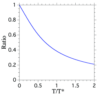
Figure 1: Ratio of the renormalized $B$ vertex to its small $\Gamma$ limit versus $T/T^{*}$ where $T^{*}$ is the pseudogap temperature, and $\Gamma/\Delta=\sqrt{3}T/T^{*}$ with the coefficient chosen so that the spectral gap disappears at $T^{*}$.

In the limit of small $\Gamma\ll\Delta$, the term in parenthesis reduces to $2\Delta/\Gamma$. Since $\Gamma\sim T$ and $\eta\sim 1/T$, then in this limit, the ratio is a constant, and one obtains the same functional form for the Nernst as in the gaussian approximation. On the other hand, as $\Gamma$ increases, the ratio decreases from unity as can be seen in Fig. 1. This leads to a Nernst signal which decays more rapidly than the gaussian result, since three renormalized $B$ vertices enter the expression for the Nernst:

$$\bar{\alpha}_{xy}=\bar{\alpha}_{xy}^{G}(B/B^{G})^{3}$$ (20)

We now consider the Nernst data for La_2-xSr_xCuO₄.Wang The advantage of these data is that after the normal carrier background has been subtracted, the Nernst signal is positive, and therefore complications due to density wave reconstruction can to first order be ignored. In Fig. 2, we show the Nernst signal, $\nu=-E_{y}/(H_{z}\nabla_{x}T)$, for four different dopings. For the overdoped compound, the gaussian expression for $\bar{\alpha}_{xy}$ fits the data quite well, but not for the three underdoped compounds where the pseudogap is present. Instead, we find that the corrected expression provides a good description of the data (with pseudogap temperatures $T^{*}$ ranging from about 200 to 300 K).

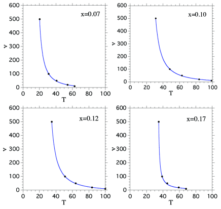
Figure 2: Nernst signal, $\nu$, versus $T$ for La_2-xSr_xCuO₄ for four different values of the doping, $x$.Wang The curve for x=0.17 is a fit to the gaussian expression for $\bar{\alpha}_{xy}$. The other curves include the vertex correction as described in this paper.

We now turn to a brief discussion of the bosonic contribution to the conductivity. As with the Nernst, the paraconductivity observed in underdoped cuprates well above $T_{c}$ falls off like $T^{-\delta}$ with $\delta\approx 3$.Leridon We recall that when extended to the higher temperature regime, gaussian theory (in 2D) predicts for the Aslamazov-Larkin RVV contribution to the conductivity $\sigma_{xx}^{AL}=e^{2}/8\pi^{2}\ln^{3}(T/T_{c})$ while for the Maki-Thompson AV-ARV contribution, $\sigma_{xx}^{MT}=\pi^{2}e^{2}\ln(1/\gamma_{\varphi})/192\ln^{2}(T/T_{c})$ where $\gamma_{\varphi}$ is the dephasing rate. In either case, the $\ln^{-n}(T/T_{c})$ decay is too slow to explain the experimental data. We now argue that the same vertex renormalization can account for the faster decay of the fluctuational conductivity. We start from the definition of the conductivity in the linear response regime $\sigma_{xx}^{AL}=-\mathrm{Im}[\Lambda_{xx}^{R}(\Omega)]/\Omega$ where the current-current response kernel is

$$\Lambda_{xx}(i\Omega_{m})=-4e^{2}T\sum_{q,\omega_{n}}B_{x}^{2}(q)L(q,i\omega_{n})L(q,i\omega_{n}+i\Omega_{m})$$ (21)

After Matsubara summation and analytic continuation, this reduces to

$$\Lambda_{xx}^{R}(\Omega) = -\frac{2e^{2}}{\pi}\sum_{q}B_{x}^{2}(q)\int_{-\infty}^{+\infty}d\omega\coth\frac{\omega}{2T}\mathrm{Im}L_{R}(q,\omega)$$ (22)

$$\times[L_{R}(q,\omega+\Omega)+L_{A}(q,\omega-\Omega)]\qquad$$

In the dc limit, we expand $L_{R}(q,\omega+\Omega)+L_{A}(q,\omega-\Omega)\simeq 2i\Omega\partial_{\omega}\mathrm{Im}L_{R}(q,\omega)$, integrate by parts over $\omega$, and as a result find for the AL contribution to the conductivity

$$\sigma_{xx}^{AL}=\frac{e^{2}}{\pi T}\sum_{q}B_{x}^{2}(q)\int_{-\infty}^{+\infty}\frac{d\omega}{\sinh^{2}\frac{\omega}{2T}}[\mathrm{Im}L_{R}(q,\omega)]^{2}$$ (23)

This is formally the same expression as in gaussian theory except for the vertex function now defined by Eq. (18). We thus find as a result (restoring $\hbar$)

$$\sigma_{xx}^{AL}=\frac{e^{2}}{16\hbar\ln(T/T_{c})}(B/B^{G})^{2}$$ (24)

where the renormalization factor $(B/B^{G})^{2}$ provides a faster power-law decay, consistent with the data.Leridon

We would like to conclude with the observation that although we assumed a ‘BCS’ expression for the pseudogap Greens function, $G$, any theory of the pseudogap with a $T$ independent d-wave like gap and a scattering rate proportional to $T$ will yield results equivalent to those derived here. Similar conclusions have been reached in regards to the fermionic contribution to various transport properties in the pseudogap phase.Alex10

In summary, we note that the Nernst signal and fluctuational conductivity for underdoped compounds drops more rapidly with temperature than predicted from a gaussian theory of fluctuating pairs. This discrepancy is nicely accounted for by a vertex correction to the fermionic current block due to the pseudogap.

This work was supported by the U. S. DOE, Office of Science, under contract DE-AC02-06CH11357. The authors acknowledge helpful discussions with M. N. Serbyn.

References

• (1) T. Timusk and B. Statt, Rep. Prog. Phys. 62, 61 (1999).
• (2) M. R. Norman, D. Pines and C. Kallin, Adv. Phys. 54, 715 (2005).
• (3) Z. A. Xu et al., Nature 406, 486 (2000).
• (4) Y. Wang et al., Phys. Rev. B 64, 224519 (2001) and Y. Wang, L. Li and N. P. Ong, Phys. Rev. B 73, 024510 (2006).
• (5) I. Ussishkin and S. L. Sondhi, Int. J. Mod. Phys. 18, 3315 (2004).
• (6) O. Cyr-Choiniere et al., Nature 458, 743 (2009); J. Chang et al., Phys. Rev. Lett. 104, 057005 (2010); R. Daou et al., Nature 463, 519 (2010).
• (7) L. Li et al., Phys. Rev. B 81, 054510 (2010).
• (8) S. Ullah and A. T. Dorsey, Phys. Rev. Lett. 65, 2066 (1990); Phys Rev. B 44, 262 (1991).
• (9) I. Ussishkin, S. L. Sondhi and D. A. Huse, Phys. Rev. Lett. 89, 287001 (2002); I. Ussishkin, Phys. Rev. B 68, 024517 (2003).
• (10) M. N. Serbyn, M. A. Skvortsov, A. A. Varlamov and V. Galitskii, Phys. Rev. Lett. 102, 0670021 (2009); K. Michaeli and A. M. Finkel’stein, Europhys. Lett. 86, 27007 (2009).
• (11) L. G. Aslamazov and A. I. Larkin, Sov. Phys. Solid State 10, 875 (1968).
• (12) M. R. Norman, M. Randeria, H. Ding and J. C. Campuzano, Phys. Rev. B 57, R11093 (1998).
• (13) J. G. Storey, J. L. Tallon, G. V. M. Williams and J. W. Loram, Phys. Rev. B 76, 060502(R) (2007).
• (14) M. R. Norman et al., Phys. Rev. B 76, 174501 (2007).
• (15) A. Kanigel et al., Nature Physics 2, 447 (2006).
• (16) A. I. Larkin and A. Varlamov, Theory of Fluctuations in Superconductors (Clarendon Press, Oxford, 2005).
• (17) Here, we have used the same heat vertex as Ussishkin et al.Uss02 so as reproduce the phenomenological Ginzburg-Landau result for the Nernst. The actual heat vertex should be twice as large as discussed by M. Yu. Reizer and A. V. Sergeev, Phys. Rev. B 50, 9344 (1994). The latter is supported by the detailed calculations of Ref. Serbyn, where the full frequency dependence of the heat vertex was kept.
• (18) In writing this expression, we have made use of the fact that since the characteristic scale of the bosonic momentum is $q\ll k_{F}$, we can set $q\rightarrow 0$ in the Cooperons, $C$, thus approximating $C(q,\varepsilon+\Omega,\omega-\varepsilon)C(q,\varepsilon,\omega-\varepsilon)\approx C^{2}(0,\varepsilon,-\varepsilon)\approx 1$.
• (19) B. Leridon et al., Phys. Rev. Lett. 87, 197007 (2001) and Phys. Rev. B 76, 012503 (2007).
• (20) L. Reggiani, R. Vaglio and A. A. Varlamov, Phys. Rev. B 44, 9541 (1991).
• (21) L. G. Aslamazov and A. A. Varlamov, J. Low Temp. Phys. 38, 223 (1980); B. L. Altshuler, M. Yu. Reizer and A. A. Varlamov, Sov. Phys. JETP 57, 1329 (1983).
• (22) A. Levchenko, T. Micklitz, M. R. Norman and I. Paul, Phys. Rev. B 82, 060502(R) (2010).