Interplay between Superconductivity and Antiferromagnetism in a Multi-layered System

Abstract

Based on a microscopic model, we study the interplay between superconductivity and antiferromagnetism in a multi-layered system, where two superconductors are separated by an antiferromagnetic region. Within a self-consistent mean-field theory, this system is solved numerically. We find that the antiferromagnetism in the middle layers profoundly affects the supercurrent flowing across the junction, while the phase difference across the junction influences the development of antiferromagnetism in the middle layers. This study may not only shed new light on material design and material engineering, but also bring important insights to building Josephson-junction-based quantum devices, such as SQUID and superconducting qubit.

I Introduction

As a remarkable aspect of high-$T_{c}$ superconductivity, its unique characteristics may result from the competition between more than one type of order parameter. PWAnderson:97 ; PALee:06 ; SChakravarty:04 Historically, the typical antagonistic relationship between superconductivity and magnetism has led researchers to avoid using magnetic elements, such as iron, as potential building blocks of superconducting (SC) material. However, it is now well accepted that the unconventional superconductivity emerging upon doping is closely related to the antiferromagnetism (AFM) in parent compounds JZaanen:89 ; KMachida:89 ; SAKivelson:03 ; EDemler:04 . Recent research theme in high-$T_{c}$ cuprate community centers on how to establish the connection between antiferromagnetic (AF) and $d$-wave SC (DSC) orderings orenstein00 , i.e., whether they compete with each other or coexist microscopically. This issue is a subject of current discussions. Depending on material details, some compounds show the coexistence of DSC and AFM YSLee:99 while others exhibit microscopic separation of these two phases SHPan:01 . Engineered heterogeneous systems and multilayered high-$T_{c}$ cuprates offer a unique setting to study the interplay between DSC and AFM. In these systems, the disorder effect can be minimized significantly with atomically smooth interfaces. Experimentally, no mixing of DSC and AFM was reported in the heterostructure artificially grown by stacking integer number of $\mathrm{La_{1.85}Sr_{0.15}CuO_{4}}$ and $\mathrm{La_{2}CuO_{4}}$ layers bozovic . Meanwhile microscopic evidence for the uniform mixed phase of AFM and DSC in outer $\mathrm{CuO_{2}}$ planes was reported mukuda on a Hg-based five-layered cuprate. Theoretically, Demler et al. phenomenalogical have studied the proximity effect and Josephson coupling in the SO(5) theory of high-$T_{c}$ superconductors. Depending on the thickness, the middle antiferromagnetic region could behave like a superconductor, metal or insulator. On the other hand, it was shown in the perturbation theory perturbative that the spin exchange coupling in the insulating AF layer can allow the tunneling of Cooper pairs.

In this article, we study microscopically a multi-layered system with two superconductors separated by AF layers. Through self-consistent mean-field theory and numerical diagonalization, we are able to solve the Hamiltonian, which allows us to study the interplay between DSC and AFM in detail. Varying some external parameters, such as the SC phase difference across the system $\delta\varphi$ and Coulomb interaction $U$ in the AF layers leads to interesting results about the interplay.

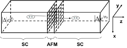
Figure 1: Schematic drawing of a multi-layered system. The middle region consists of AF layers (in X-Y plane) and the two sides are SC layers with $d$-wave pairing symmetry. The phases of the SC order parameter (or the pairing potential) in the first (far left) and the last (far right) layer are fixed at $\varphi_{L}$ and $\varphi_{R}$, respectively.

II Model and setup

The model system under consideration is schematically presented in Fig. 1, for which the Hamiltonian can be written as:

$$H = -\sum_{i,j,\sigma}t_{i,j}c_{i,\sigma}^{\dagger}c_{j,\sigma}+\sum_{i}U_{i}(n_{i,\uparrow}-\frac{1}{2})(n_{i,\downarrow}-\frac{1}{2})$$ (1)

$$-\frac{1}{2}\sum_{i,j}V_{ij}n_{i}n_{j}-\mu\sum_{i}n_{i}\;,$$

where $t_{i,j}$ denotes the hopping integral between the nearest neighbor sites. For in-plane (X-Y plane) hopping, $t_{i,j}=t$, and for inter-layer (Z direction) hopping, $t_{i,j}=t_{\perp}$. $c_{i,\sigma}$ ($c_{i,\sigma}^{\dagger}$) is the annihilation (creation) operator of electrons on the $i$th lattice site with spin $\sigma$ ($\sigma=\uparrow,\downarrow$). The quantity $n_{i,\sigma}=c_{i,\sigma}^{\dagger}c_{i,\sigma}$ is the number operator on the $i$th lattice site. Both $U_{i}$ and $V_{ij}$ are positive. $U_{i}$ indicates the on-site repulsive Coulomb interaction, which is nonzero only in the middle layers, and $V_{ij}$ describes the in-plane nearest neighbor attractive interaction, which is nonzero only in the SC layers. We are going to fix the phase of the SC order parameter in the first (far left) and the last (far right) layer at $\varphi_{L}$ and $\varphi_{R}$, respectively, which can be introduced by a gauge flux.

When there is no inter-layer coupling, $t_{\perp}=0$, the system is decomposed into individual two-dimensional (2D) systems. It is known that in a 2D SC layer, the in-plane nearest neighbor attractive interaction $V_{ij}$ leads to a nonzero energy gap $\Delta$ with $d$-wave symmetry, and in a 2D AF layer the on-site repulsive interaction $U_{i}$ leads to a nonzero $(\pi,\pi)$ spin density wave (SDW) order. In a genuine cuprate compound, there exists the inter-layer coupling, which is usually weaker than the in-plane hopping. Because of the inter-layer coupling, there arises interesting interplay between SC layers and AF layers (see Fig. 1).

The strategy of solving the Hamiltonian is briefly summarized as follows: Due to the translational symmetry in the 2D X-Y plane, the 3D problem can be decomposed into a 2D (X-Y) plus 1D (Z) problem. In the X-Y plane, $\vec{k}=(k_{x},k_{y})$ is a good quantum number, where $k_{x}=\frac{1}{2}(\frac{n_{x}}{N_{x}}-\frac{n_{y}}{N_{y}})\pi$, $k_{y}=\frac{1}{2}(\frac{n_{x}}{N_{x}}+\frac{n_{y}}{N_{y}})\pi$, and $n_{x}=-\frac{1}{2}N_{x}$, $-\frac{1}{2}N_{x}+1$, $\cdots$, $\frac{1}{2}N_{x}-1$, $n_{y}=-\frac{1}{2}N_{y}$, $-\frac{1}{2}N_{y}+1$, $\cdots$, $\frac{1}{2}N_{y}-1$. In order to simplify the Hamiltonian, we adopt the mean-field approximation, which leads to the following Bogoliubov-de Gennes equation PGdeGennes:1965 :

$$\sum_{m}\left[\begin{array}[]{cccc}\xi_{\vec{k}n}\delta_{nm}+t_{nm}&-\frac{U_{n}}{2}M_{n}\delta_{nm}&\Delta_{\vec{k},n}\delta_{nm}&0\\ -\frac{U_{n}}{2}M_{n}\delta_{nm}&\xi_{\vec{k}+\vec{Q},n}\delta_{nm}+t_{nm}&0&\Delta_{\vec{k}+\vec{Q},n}\delta_{nm}\\ \Delta_{\vec{k},n}^{\ast}\delta_{nm}&0&-\xi_{-\vec{k}n}\delta_{nm}-t_{nm}^{\ast}&-\frac{U_{n}}{2}M_{n}\delta_{nm}\\ 0&\Delta_{\vec{k}+\vec{Q},n}^{\ast}\delta_{nm}&-\frac{U_{n}}{2}M_{n}\delta_{nm}&-\xi_{-(\vec{k}+\vec{Q})n}\delta_{nm}-t_{nm}^{\ast}\\ \end{array}\right]\left[\begin{array}[]{c}u_{\vec{k},m,\uparrow}^{\alpha}\\ u_{\vec{k}+\vec{Q},m,\uparrow}^{\alpha}\\ v_{\vec{k},m,\downarrow}^{\alpha}\\ v_{\vec{k}+\vec{Q},m,\downarrow}^{\alpha}\end{array}\right]=E_{\alpha}\left[\begin{array}[]{c}u_{\vec{k},n,\uparrow}^{\alpha}\\ u_{\vec{k}+\vec{Q},n,\uparrow}^{\alpha}\\ v_{\vec{k},n,\downarrow}^{\alpha}\\ v_{\vec{k}+\vec{Q},n,\downarrow}^{\alpha}\end{array}\right]\;,$$ (2)

where $m$ and $n$ label the layer number; $\vec{k}$ and $\vec{k}+\vec{Q}$ with $\vec{Q}=(\pi,\pi)$ denote the wave vectors in the first Brillouin zone of the X-Y plane, $t_{mn}=t_{\perp}(\delta_{n,m+1}+\delta_{n,m-1})$ describes the nearest neighbor inter-plane hopping, $\xi_{\vec{k}n}=-2t(\cos k_{x}+\cos k_{y})-\mu$ is the normal metal dispersion relation, $\mu$ is the chemical potential, the variables $U_{n}$ is equal to $U$ in the AF layers and zero otherwise while $V_{n}$ is equal to $V$ in the SC layers and zero otherwise. The superconducting pairing potential $\Delta_{\vec{k},n}=V_{n}\Psi_{n}(\cos k_{x}-\cos k_{y})/2$, where $\Psi_{n}$ is the superconducting pairing wavefunction. Obviously, the superconducting pairing potential, which is the SC order parameter has the same phase as that of the superconducting pairing wavefunction. $M_{n}=\left\langle n_{n,\uparrow}\right\rangle-\left\langle n_{n,\downarrow}\right\rangle$ describes the SDW in the $n$-th layer. The average electron number $\left\langle n_{n,\uparrow}\right\rangle$, $\left\langle n_{n,\downarrow}\right\rangle$ and the SC pairing wavefunction $\Psi_{n}$ can be determined self-consistently through iteration over the following relation:

$$\Psi_{n}=\frac{2}{N}\sum_{\vec{k},\alpha}\frac{(\cos k_{x}-\cos k_{y})}{2}g(u,v)\tanh{\frac{\beta E_{\alpha}}{2}}\;,$$ (3a)

$$\left\langle n_{n,\uparrow}\right\rangle=\frac{1}{N}\sum_{\vec{k},\alpha}\left|u_{\vec{k},n,\uparrow}^{\alpha}+u_{\vec{k}+\vec{Q},n,\uparrow}^{\alpha}\right|^{2}f(E_{\alpha})\;,$$ (3b)

$$\left\langle n_{n,\downarrow}\right\rangle=\frac{1}{N}\sum_{\vec{k},\alpha}\left|v_{\vec{k},n,\downarrow}^{\alpha}+v_{\vec{k}+\vec{Q},n,\downarrow}^{\alpha}\right|^{2}f(-E_{\alpha})\;,$$ (3c)

where $N=N_{x}\times N_{y}$ is the sites number in a 2D plane. $\vec{k}$ samples half of the first Brillouin zone. $g(u,v)=u_{\vec{k},n,\uparrow}^{\alpha}v_{\vec{k},n,\downarrow}^{\alpha,\ast}-u_{\vec{k}+\vec{Q},n,\uparrow}^{\alpha}v_{\vec{k}+\vec{Q},n,\downarrow}^{\alpha,\ast}$, and $f(E_{\alpha})=1/(1+e^{\beta E_{\alpha}})$ is the Fermi distribution. Through this simplification, the multi-layered system is then solved numerically. We are especially interested in the interplay between the DSC and the AFM, which is characterized by the SDW $M_{n}$ and the SC pairing wavefunction $\Psi_{n}$. We will focus on zero temperature $T=0$. The size of X-Y plane is $N_{x}=N_{y}=40$. The total layer number is $N_{z}=22$. The two middle layers are AF layers ($U_{n}=U$, $V_{n}=0$, for $n=11$, $12$), and the rest are SC layers ($U_{n}=0$, $V_{n}=V$, for $n=1$, $2$, $\cdots$, $10$, and $n=13$, $\cdots$, $22$). For simplicity, we choose $t=1$, $t_{\perp}=0.1$, $V=1.5$, and $\mu=0$. We will vary the control parameters, such as $U$ and $\delta\varphi=\varphi_{L}-\varphi_{R}$, to study the competition between DSC and AFM. When the phase difference $\delta\varphi$ is introduced, there is a current flowing across the system and its expression is given by:

$$I = 2\frac{t_{\perp}e}{N}\sum_{\vec{k},\alpha}\mathrm{Im}\biggl{\{}\left[u_{\vec{k},n,\uparrow}^{\alpha,\ast}u_{\vec{k},n+1,\uparrow}^{\alpha}+\left(\vec{k}\leftrightarrow\vec{k}+\vec{Q}\right)\right]f_{+}$$ (4)

$$+\left[v_{\vec{k},n,\downarrow}^{\alpha}v_{\vec{k},n+1,\downarrow}^{\alpha,\ast}+v_{\vec{k}+\vec{Q},n,\downarrow}^{\alpha}v_{\vec{k}+\vec{Q},n+1,\downarrow}^{\alpha,\ast}\right]f_{-}\biggr{\}}\;,$$

where $f_{\pm}=f(\pm E_{\alpha})$.

III Influence of antiferromagnetism on superconductivity

In the model introduced above, the change of the Coulomb interaction $U$ in the middle layers can drive a metal-Mott insulator phase transition at a certain value $U_{c}$. Correspondingly, the multi-layered system changes from a superconductor/normal metal/superconductor (SNS) weak link bardeen72 to a superconductor/insulator/superconductor (SIS) Josephson junction josephson . The studies of SNS and SIS junctions with static potential barrier have been well documented bardeen72 ; josephson ; MTinkham:75 . Here we start from a microscopic model and drive the middle layers to change from one electronic state into another by tuning the on-site Coulomb interaction $U$. We are interested in how the SC pairing wavefunction and the current across the junction change with the Coulomb interaction $U$. We plot the current as a function of the phase difference $\delta\varphi$ in Fig. 2. It can be seen that below a threshold value of $U_{c}\approx 0.8$, the current is a piecewise periodic function. In each periodic region, it varies linearly with $\delta\varphi$. This agrees with the result obtained in Ref. bardeen72, for a junction with a normal metal. We also find that when the Coulomb interaction is larger than $U_{c}$, the current as a function of $\delta\varphi$ changes gradually with the increase of $U$. When $U$ is in the range $0.8<U<1.5$, the current shows a shape intermediate between a piecewise linear function and a sinusoidal function. Similar results have been observed in Refs. bardeen72 ; phenomenalogical ; EDemler:04 when one varies the temperature or the thickness of the middle layers instead of the the Coulomb interaction $U$. When $U\approx 2.0$, the current is well approximated by a sinusoidal function of $\delta\varphi$ (see Fig. 2), which is a typical feature of the dc Josephson junction (JJ) current josephson . The magnitude of current decreases rapidly with the increase of $U$.

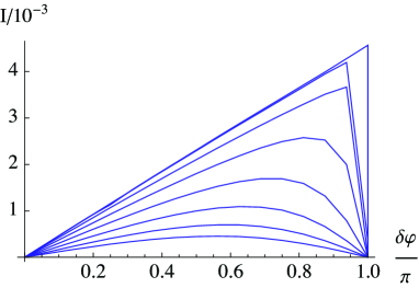
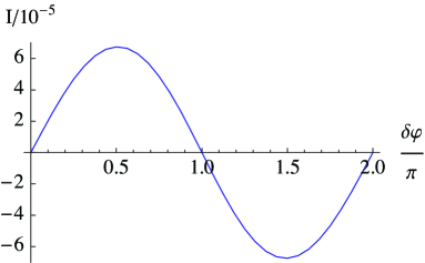
Figure 2: Current across the junction as a function of the phase difference $\delta\varphi$ of two superconductors for different $U$. Here $V=1.5$, $t_{\perp}=0.1$, $N_{x}=N_{y}=40$, $N_{z}=22$. Up panel: $U=0$, $0.1$, $0.2$, $\cdots$, $1.5$, and $\delta\varphi=0\sim\pi$. Down panel: $U=2.0$ and $\delta\varphi=0\sim 2\pi$.

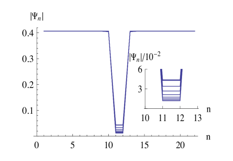
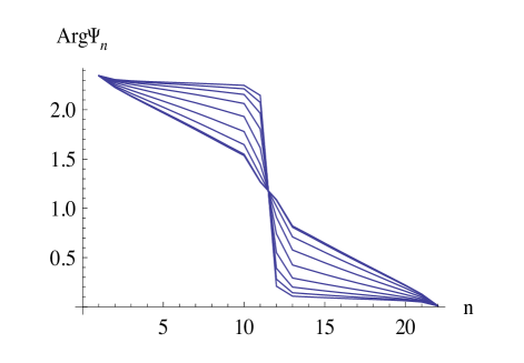
Figure 3: Absolute value (Up panel) and argument (Down panel) of superconducting pairing wavefunction $\Psi_{n}$ as a function of layer number. The phase of SC pairing wavefunction is the same as that of the pairing wavefunction. Here $V=1.5$, $t_{\perp}=0.1$, $N_{x}=N_{y}=40$, $N_{z}=22$, $\delta\varphi=3\pi/4$. $U$ is fixed at different values: $U=0$, $0.1$, $0.2$, $\cdots$, $1.5$.

In order to have a better understanding of the influence of AFM on DSC, we plot the absolute value and the phase of the SC pairing wavefunction in Fig. 3. It can be seen that when $U$ is small, there is a nonzero paring potential in the middle layers due to the proximity effect, and the two superconductors are weakly linked by the normal metallic layers. In this weak link regime, the phase of the SC pairing wavefunction is almost linear in layer number $n$. This means that when the middle layers are in the normal metallic state, it has little influence on the SC layers on two sides. However, when $U$ is larger than $U_{c}\approx 0.8$, SDW develops, and the middle layers become Mott insulator. Quantum mechanically, Cooper pairs can still tunnel through the SDW region when $U$ is not very large. We call this intermediate $U$ regime as the tunneling regime. From the weak link regime to tunneling regime, the phase of the SC paring wavefunction changes gradually from a (nearly) linear function to a step function of the layer number (see Fig. 3). This corresponds to the observation that the current shape changes from being piecewise linear to sinusoidal. Therefore, when $U$ is very large, the current-phase relation becomes identical to the famous Josephson relation josephson ; feynman . Here for the first time, we establish the connection between the profile of the SC phase distribution (Fig. 3) and the current-phase dependence (Fig. 2), which we believe is rather intriguing.

When one continues to increase $U$, the middle layers becomes more opaque and the superconducting pairing wavefunction is completely suppressed in this region. As a result, the tunneling of Cooer pairs will be completely quenched, and the two comprising superconductors become decoupled.

We also would like to mention that when the middle layers are in the normal metallic state, the current across the junction is a mesoscopic effect JXZhu:10 . The current is proportional to the phase gradient of the SC pairing wavefunction. That is, when one increases the number of SC layers, the current will decrease and finally vanish. However, when the middle layer is in the AF state, the whole system becomes a JJ. The current of a JJ is no longer a mesoscopic effect. It is completely determined by the phase difference of the SC pairing wavefunction on both ends of the system. Therefore, it will not decrease with the increase of the number of the SC layers. In this sense we say that AFM insulator layers enhance supercurrent.

IV Influence of superconductivity on antiferromagnetism

In the above discussion, we find the profound influence of the Coulomb interaction $U$ (and hence AFM) of the middle layers on the DSC. We now study the back-action of DSC on AFM. We will fix the phase difference $\delta\varphi$ at different values, and see if the SDW in the middle layers changes with $\delta\varphi$. We plot in Fig. 4 the SDW as a function of $U$ for various values of $\delta\varphi$. Clearly, the SDW in the middle layers is influenced by $\delta\varphi$ in certain range of $U$. When $\delta\varphi=\pi$, the critical value $U_{c}$, after which the SDW develops, is much smaller than in the case of $\delta\varphi=0$, though the current is zero in both cases. This is very similar to the result in Ref. phenomenalogical, that the middle AF layers will be influenced by the current fed into the junction. When the Coulomb interaction is very weak, the SDW does not develop for $\delta\varphi\neq\pi$, and the middle layers are in the normal metallic state. In contrast, when the Coulomb interaction is very strong, e.g. $U>1.2$, the AFM is robust against the phase difference across the junction and strongly suppresses the pairing wavefunction in the middle region (see Fig. 3). Only when $U$ is small, is the emergence of the SDW sensitive to the phase difference.

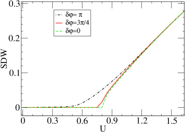
Figure 4: (Color online) SDW in the middle layer ($n=11$) as a function of the Coulomb interaction for different fixed $\delta\varphi$. Here $U=0\sim 1.5$, $V=1.5$, $t_{\perp}=0.1$, $N_{x}=N_{y}=40$, $N_{z}=22$, $\delta\varphi=0$ (solid), $3\pi/4$ (dashed), and $\pi$ (dot dashed).

When switching off the interlayer coupling ($t_{\perp}=0$), the system is decoupled into 2D systems. The DSC on two sides will not influence the AFM in the middle layer. The middle layer is described by a 2D Hubbard model, in which the SDW will develop for an infinitesimal $U$. In the present model ($t_{\perp}\neq 0$), when $\delta\varphi=0$, the SDW in the middle layers is suppressed due to the inter-layer coupling, which weakens the perfect nesting at $\vec{Q}=(\pi,\pi)$. The SDW will not develop until $U$ is larger than a threshold value $U_{c}$ (see Fig. 4). Hence both $t_{\perp}$ and $\delta\varphi$ will influence the AFM. The results in Fig. 4 indicate that the AFM shows a crossover behavior for $\delta\varphi=\pi$ rather than a criticality as obtained for $\delta\varphi=0$. For $\delta\varphi\in(0,\pi)$, the SDW critical point $U_{c}$ is less than that for $\delta\varphi=0$. This result is in agreement with that in Ref. phenomenalogical, .

In order to have a better understanding of the influence of the DSC on the AFM in the middle layers, we plot in Fig. 5 the local density of state (LDOS), as given by

$$\rho_{n,\uparrow}(E) = \frac{1}{N}\sum_{\vec{k},\alpha}\left|u_{\vec{k},n,\uparrow}^{\alpha}+u_{\vec{k}+\vec{Q},n,\uparrow}^{\alpha}\right|^{2}\left[-\frac{\partial f(\omega)}{\partial\omega}\right],$$ (5a)

$$\rho_{n,\downarrow}(E) = \frac{1}{N}\sum_{\vec{k},\alpha}\left|v_{\vec{k},n,\downarrow}^{\alpha}+v_{\vec{k}+\vec{Q},n,\downarrow}^{\alpha}\right|^{2}\left[-\frac{\partial f(\omega^{\prime})}{\partial\omega^{\prime}}\right],$$ (5b)

where $\omega=E-E_{\alpha}$ and $\omega^{\prime}=E+E_{\alpha}$. From Fig. 5, we can see a sharp intensity decay of LDOS at $E_{F}$ when $\delta\varphi=0$. When $\delta\varphi=\pi$, the LDOS exhibits a peak structure at $E_{F}$. Since the development of the SDW is also determined by the normal-state DOS at low energies, it explains the different SDW critical behavior between the cases with $\delta\varphi=\pi$ and $\delta\varphi=0$.

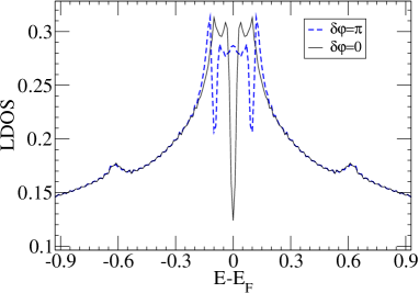
Figure 5: (Color online) LDOS of the middle layer ($n=11$) $\rho_{11,\uparrow}(E)$. Here $U=0$, $V=1.5$, $t_{\perp}=0.1$, $N_{x}=N_{y}=40$, $N_{z}=22$, $\delta\varphi=0$, and $\pi$.

V Conclusion and discussion

We have studied the interplay between the DSC and AFM in a multi-layered system. It is revealed that the AF layers have profound influence on the DSC. A metal-Mott insulator phase transition makes the multi-layer system change from a SNS to a SIS junction. We have also established the connection between the profile of the SC phase distribution and the current-phase dependence. We find that when the barrier of the middle layers is not high enough (metal or semiconductor regime), the middle layers cannot maintain a step-function-like phase of two superconductors on two sides. Accordingly, the current across the junction will deviate from a sinusoidal function of the phase difference. When the barrier of the middle layer is high (deep insulator regime), as predicted by Josephson josephson the phase across the junction is a step function, and the current is a sinusoidal function of the phase difference. Meanwhile, the phase difference across the system will dramatically influence the development of SDW in the middle layers. The results from our simulations may shed new light on material engineering. The DSC and AFM can coexist in a single layer, but they also compete with each other. Another important insight from the present study is the microscopic model of JJ. JJ has been widely used in a lot of quantum devices, such as in SQUID for ultra-sensitive magnetic field measurement and superconducting qubit qubit for quantum computing. Our study provides a microscopic theory for JJ, hence has possible applications in building adaptive JJ based devices by engineering the middle layers of the JJ. Finally, with the development of experimental techniques, it is now possible to synthesize heterogeneous systems with layer by layer at atomic scale threelayer . We expect that our results can be experimentally verified, as some experiments on engineered material have been reported threelayer ; bozovic ; mukuda .

Acknowledgments: We thank A. V. Balatsky, Quanxi Jia, A. J. Taylor, and S. Trugman for useful discussions. This work was carried out under the auspices of the National Nuclear Security Administration of the U.S. DOE at LANL under Contract No. DE-AC52-06NA25396, the LANL LDRD-DR Project X96Y, and the U.S. DOE Office of Science.

References

- (1) P. W. Anderson, The Theory of Superconductivity in the High- Cuprate Superconductors (Princeton University, Princeton, 1997).
- (2) P. A. Lee, N. Nagaosa, and X.-G. Wen, Rev. Mod. Phys. 78, 17 (2006).
- (3) S. Chakravarty, H.-Y. Kee, and K. Völker, Nature 428, 53 (2004).
- (4) J. Zaanen and O. Gunnarsson, Phys. Rev. B 40, R7391 (1989).
- (5) K. Machida, Physica C (Amsterdam) 158, 192 (1989).
- (6) S. A. Kivelson, I. P. Bindloss, E. Fradkin, V. Oganesyan, J. M. Tranquada, A. Kapitulnik and C. Howald, Rev. Mod. Phys. 75, 1201 (2003).
- (7) E. Demler, W. Hanke, and S.-C. Zhang, Rev. Mod. Phys. 76, 909 (2004).
- (8) J. Orenstein and A. J. Millis, Science 288, 468 (2000).
- (9) Y. S. Lee, R. J. Birgeneau, M. A. Kastner, Y. Endoh, S. Wakimoto, K. Yamada, R. W. Erwin, S.-H. Lee, and G. Shirane, Phys. Rev. B 60, 3643 (1999).
- (10) S. H. Pan, J. P. O’Neal, R. L. Badzey, C. Chamon, H. Ding, J. R. Engelbrecht, Z. Wang, H. Eisaki, S. Uchida, A. K. Gupta, K.-W. Ng, E. W. Hudson, K. M. Lang and J. C. Davis, Nature (London) 413, 282 (2001).
- (11) I. Bozovic, G. Logvenov, M. A. J. Verhoeven, P. Caputo, E. Goldobin and T. H. Geballe, Nature (London) 422, 873 (2003).
- (12) H. Mukuda, M. Abe, Y. Araki, Y. Kitaoka, K. Tokiwa, T. Watanabe, A. Iyo, H. Kito, and Y. Tanaka, Phys. Rev. Lett. 96, 087001 (2006).
- (13) E. Demler, A. J. Berlinsky, C. Kallin, G. B. Arnold, and M. R. Beasley, Phys. Rev. Lett. 80, 2917 (1998).
- (14) M. Mori and S. Maekawa, Phys. Rev. Lett. 94, 137003 (2005).
- (15) P. G. de Gennes, Superconductivity of Metals and Alloys (Benjamin, New York, 1965).
- (16) J. Bardeen and J. L. Johnson, Phys. Rev. B 5, 72 (1972).
- (17) B. D. Josephson, Phys. Lett. 1, 251 (1962).
- (18) M. Tinkham, Introduction to Superconductivity (McGraw-Hill, New York, 2nd Ed., 1996).
- (19) R. P. Feynman, Lectures on Physics (Addison-Wesley, Reading, MA, 1963); D. Rogovin, M. O. Scully, Ann. Phys. 88, 371 (1974).
- (20) J.-X. Zhu and H. T. Quan, Phys. Rev. B 81, 054521 (2010).
- (21) J. Q. You and F. Nori, Phys. Today 58, No. 11, 42 (2005); J. Clarke and F. K. Wilhelm, Nature. 453, 1031 (2008).
- (22) M. Karppinen, and H. Yamauchi, Material Sci. Eng. 26 51 (1999).