Topological Lattice Actions

Abstract

We consider lattice field theories with topological actions, which are invariant against small deformations of the fields. Some of these actions have infinite barriers separating different topological sectors. Topological actions do not have the correct classical continuum limit and they cannot be treated using perturbation theory, but they still yield the correct quantum continuum limit. To show this, we present analytic studies of the 1-d $O(2)$ and $O(3)$ model, as well as Monte Carlo simulations of the 2-d $O(3)$ model using topological lattice actions. Some topological actions obey and others violate a lattice Schwarz inequality between the action and the topological charge $Q$. Irrespective of this, in the 2-d $O(3)$ model the topological susceptibility $\chi_{t}=\langle Q^{2}\rangle/V$ is logarithmically divergent in the continuum limit. Still, at non-zero distance the correlator of the topological charge density has a finite continuum limit which is consistent with analytic predictions. Our study shows explicitly that some classically important features of an action are irrelevant for reaching the correct quantum continuum limit.

1 Introduction

Universality is a key concept in classical statistical mechanics and in quantum field theory. In particular, in lattice field theory numerous lattice actions yield the same universal continuum limit. It is well known that locality is vital for the viability of universality. A universality class is characterized by the space-time dimension and the symmetries of the relevant fields. In order to construct lattice theories that fall into a desired universality class, one often imposes additional features of the corresponding classical theory on the lattice action. Usually one constructs a lattice action by replacing derivatives of the continuum fields by finite differences of the lattice fields. Such a discretization ensures the correct classical continuum limit. In addition, the lattice theory can then be investigated using perturbation theory. For example, for QCD it has been proved rigorously that the lattice regularization yields the same continuum limit as perturbative regularization schemes, such as dimensional regularization [1, 2]. Taking advantage of universality, and following Symanzik’s improvement program [3, 4], one can systematically construct improved lattice actions [5, 6] which eliminate lattice artifacts up to a given order in the lattice spacing. At a fixed point of the renormalization group, so-called classically perfect lattice actions have been constructed, which are free of lattice artifacts at the classical level [7, 10, 8, 9]. In particular, in asymptotically free theories, including QCD and the 2-d $O(3)$ model, a classically perfect fixed point action has been constructed by solving a minimization problem. In this paper, we proceed in a very different direction. In order to test the robustness of universality, we explicitly violate classically important properties of the action, such as the classical continuum limit, the applicability of perturbation theory, or the Schwarz inequality between the action and the topological charge. Hence, in contrast to Symanizik’s lattice actions, which may, for example, be 1-loop improved, the actions that we will study can be viewed as tree-level impaired, but they are certainly still local. As we will see, even without appropriate classical features, the lattice theory acquires the correct quantum continuum limit. This also holds in one dimension (i.e. in quantum mechanics), although in this case one does usually not rely on universality. From the point of view of Wilson’s renormalization group applied to critical phenomena the irrelevance of classical features of a given lattice action is perhaps not too surprising. For example, it is well known that the 4-d Ising model, whose classical Hamiltonian does not have a meaningful continuum limit, is in the same universality class as the $\phi^{4}$ quantum field theory.

We will investigate local lattice actions that are invariant against small continuous deformations of the lattice fields. Such actions — which we will call topological lattice actions — have infinitely many flat directions because they do not suppress small field fluctuations. As a consequence, they do not have the correct classical continuum limit and perturbation theory is not applicable. Depending on the nature of a topological action, it may or may not obey a Schwarz inequality. In this paper, we study two different types of topological lattice actions. The first one constrains the angle $\varphi$ between nearest-neighbor $O(N)$ spins to $|\varphi|<\delta$. All field configurations that satisfy this constraint have the same action value $S=0$. Besides not having the correct classical continuum limit, this lattice action violates the Schwarz inequality between action and topological charge. The quantum continuum limit is reached by sending the maximally allowed angle $\delta$ to zero. Patrascioiu and Seiler [11] as well as Aizenman [12] have used an action with an angle constraint to simplify the proof of the existence of a massless phase in the 2-d $O(2)$ model. Furthermore, Patrascioiu and Seiler have also used an angle-constraint action in their search for a massless phase in the 2-d $O(3)$ model [13, 14], while Hasenbusch used the same action to argue that ${\mathbb{R}P}(N-1)$ models are in the same universality class as $O(N)$ models [15]. Refs. [13, 14, 15] presented numerical evidence that the action with the angle constraint falls in the same universality class as the standard action. Our study will confirm these results and will extend them by studying the cut-off effects of this topological action, as well as by investigating the topological susceptibility and the correlator of the topological charge density. Lattice actions with a similar constraint have also been used in [16, 17, 18, 19, 20, 21, 22, 23, 24], however, not with an emphasis on the topological properties of some of these actions. The second topological lattice action that we consider receives local contributions from the absolute value of the topological charge density. This action does not have the correct classical continuum limit either, but it obeys a lattice Schwarz inequality. Irrespective of this, as we will see, the correct quantum continuum limit is reached for both topological actions.

It should be pointed out that lattice theories with topological actions are not regularizations of the topological field theories that arise in the context of string theory or conformal field theory [25]. While those theories realize new universality classes, the theories with topological lattice actions studied here fall into standard universality classes, despite the fact that they violate basic principles of classical physics.

The $O(N)$ model in $(N-1)$ dimensions has a non-trivial topological charge $Q\in\Pi_{N-1}[S^{N-1}]={\mathbb{Z}}$. We will investigate the 1-d $O(2)$ and the 2-d $O(3)$ model which have topological charges in $\Pi_{1}[S^{1}]$ and $\Pi_{2}[S^{2}]$, respectively. While the 1-d $O(2)$ model will be studied analytically, the 2-d $O(3)$ model is investigated using Monte Carlo simulations. The 2-d $O(3)$ model can also be viewed as the $N=2$ member of the 2-d ${\mathbb{C}P}(N-1)$ model family [26]. The ${\mathbb{C}P}(N-1)$ manifold is the coset space $SU(N)/U(N-1)=S^{2N-1}/S^{1}$. Since $\Pi_{2}[S^{2N-1}]=\{0\}$, one obtains $\Pi_{2}[{\mathbb{C}P}(N-1)]=\Pi_{1}[S^{1}]={\mathbb{Z}}$, i.e. all 2-d ${\mathbb{C}P}(N-1)$ models possess a non-trivial topological charge. Since they are asymptotically free, have an anomalously broken classical scale invariance and a dynamically generated mass gap, as well as instantons and $\theta$-vacuum states, 2-d ${\mathbb{C}P}(N-1)$ models share many features with 4-d Yang-Mills theories. This has motivated their detailed study beyond perturbation theory. The $\theta$-vacuum physics of 4-d $SU(N)$ gauge theories and of 2-d ${\mathbb{C}P}(N-1)$ models has been reviewed in [27].

Topological aspects of lattice ${\mathbb{C}P}(N-1)$ models have been investigated in [28, 29, 30, 31, 32, 17, 33, 8, 34, 9, 35]. Depending on the lattice action and the lattice definition of the topological charge, the quantum continuum limit of the topological susceptibility $\chi_{t}=\langle Q^{2}\rangle/V$, where $V$ is the space-time volume, may be spoiled by short-distance lattice artifacts. These so-called dislocations have topological charge $|Q|=1$ and a minimal value of the lattice action. Semi-classical arguments, which are, however, not rigorous, suggest that $\chi_{t}$ may have a power-law divergence in the quantum continuum limit [29]. This is expected to happen in the ${\mathbb{C}P}(2)$ model, when one uses the standard action in combination with the geometric definition of the topological charge [32]. This problem does not arise for ${\mathbb{C}P}(N-1)$ models with $N\geq 4$. Even in the ${\mathbb{C}P}(2)$ case, dislocations can be eliminated and the proper continuum limit of $\chi_{t}$ can be attained if one uses a modified lattice action [32]. Dislocations have also been identified in 4-d lattice Yang-Mills theory [36, 37, 38]. Again, semi-classical arguments suggest that they may spoil the quantum continuum limit in $SU(2)$ and $SU(3)$ Yang-Mills theory, if the standard Wilson action is used in combination with the geometric definition of the topological charge [16, 36, 39, 40, 41]. As in the ${\mathbb{C}P}(2)$ model, dislocations can be eliminated in $SU(2)$ and $SU(3)$ Yang-Mills theory by using an improved lattice action [38]. The situation is more subtle in the 2-d $O(3)$ (or equivalently ${\mathbb{C}P}(1)$) model. In this case, a semi-classical calculation in the continuum already yields a divergent topological susceptibility $\chi_{t}$ even in a small space-time volume [30]. This divergence is not caused by lattice artifacts, but is an intrinsic feature of the theory in the continuum limit. Hence, one concludes that a meaningful quantum continuum limit of $\chi_{t}$ does not exist in the 2-d $O(3)$ model. This is supported by a calculation of $\chi_{t}$ using a classically perfect lattice action in combination with a classically perfect topological charge [33], which eliminates dislocations and indeed shows no power-like divergence of the topological susceptibility. However, $\chi_{t}$ still diverges logarithmically, and thus a meaningful quantum continuum limit is not reached for this quantity. As we will see, the logarithmic divergence of $\chi_{t}$ even arises for topological actions, although in that case one might have expected a power-law divergence due to dislocations. On the other hand, the correlator of the topological charge density will turn out to have a finite continuum limit. The concepts of classical and even quantum perfect definitions of the topological charge have also been investigated analytically in the 1-d $O(2)$ model [42].

In QCD, Ginsparg-Wilson lattice quarks [43] obey an Atiyah-Singer index theorem even at finite lattice spacing [44]. Based on Ginsparg-Wilson lattice fermions, unambiguous definitions of the topological susceptibility which are free of short-distance singularities have been provided [45, 46]. They have been used in a derivation of the Witten-Veneziano formula [47, 48, 49] for the $\eta^{\prime}$-meson mass in a fully regularized non-perturbative framework [50, 51, 52].

This paper is organized as follows. Section 2 contains an analytic investigation of the 1-d $O(2)$ model using two different topological lattice actions: one that suppresses topological charges and one that does not. In both cases, the correct quantum continuum limit is obtained. In Section 3 we study the 1-d $O(3)$ model in a similar manner. Section 4 presents a Monte Carlo study of the 2-d $O(3)$ model. Again, we use two different topological lattice actions: one that does and one that does not obey a Schwarz inequality. As before, the correct quantum continuum limit is reached in both cases. The Monte Carlo data for the topological susceptibility are consistent with a logarithmic divergence, while the correlator of the topological charge density has a finite continuum limit. We summarize our results and draw conclusions in Section 5.

2 The 1-d $O(2)$ Model

In this section we consider the 1-d $O(2)$ model as an analytically solvable test case with two different topological lattice actions: one that explicitly suppresses topological charges and one that does not. Remarkably, irrespective of this, and although the lattice theories do not yield the correct classical limit, they do have the correct quantum continuum limit.

2.1 The 1-d $O(2)$ Model in the Continuum

In this subsection, we analytically solve the 1-d $O(2)$ model in the continuum. The results will then be compared with those of the corresponding lattice models. The 1-d $O(2)$ model is equivalent to a quantum mechanical rotor. Let us consider a particle of mass $M$ on a circle of radius $R$, and thus with the moment of inertia $I=MR^{2}$. The Hamilton operator takes the form

$$H(\theta)=-\frac{1}{2I}\left(\partial_{\varphi}-i\frac{\theta}{2\pi}\right)^{2},$$ (2.1)

where $\varphi$ is the angle describing the position of the particle, and $\theta$ is analogous to the vacuum angle in QCD. At finite temperature $T=1/\beta$, the corresponding Euclidean continuum action is given by

$$S[\varphi]=\int_{0}^{\beta}dt\ \frac{I}{2}\dot{\varphi}^{2}-i\theta Q[\varphi],$$ (2.2)

where the topological charge takes the form

$$Q[\varphi]=\frac{1}{2\pi}\int_{0}^{\beta}dt\ \dot{\varphi}\in\Pi_{1}[S^{1}]={\mathbb{Z}}.$$ (2.3)

The energy eigenfunctions of the Hamilton operator $H(\theta)$ are given by

$$\langle\varphi|m\rangle=\frac{1}{\sqrt{2\pi}}\exp(im\varphi),$$ (2.4)

where $m\in{\mathbb{Z}}$ specifies the angular momentum, and the corresponding energy eigenvalues are

$$E_{m}(\theta)=\frac{1}{2I}\left(m-\frac{\theta}{2\pi}\right)^{2}.$$ (2.5)

The canonical partition function takes the form

$$Z(\theta)=\mbox{Tr}\exp(-\beta H(\theta))=\sum_{m\in{\mathbb{Z}}}\exp(-\beta E_{m}(\theta)).$$ (2.6)

The (not yet normalized) distribution of the topological charge $Q$ is obtained as a Fourier transform of $Z(\theta)$

$$p(Q)=\frac{1}{2\pi}\int_{-\pi}^{\pi}d\theta\ Z(\theta)\exp(-i\theta Q)=\sqrt{\frac{2\pi I}{\beta}}\exp\left(-\frac{2\pi^{2}I}{\beta}Q^{2}\right),$$ (2.7)

and the topological susceptibility (evaluated at $\theta=0$) reads

$$\chi_{t}=\frac{\langle Q^{2}\rangle}{\beta}=\frac{1}{\beta}\frac{\sum_{Q\in{\mathbb{Z}}}Q^{2}p(Q)}{\sum_{Q\in{\mathbb{Z}}}p(Q)}.$$ (2.8)

In the zero temperature limit $\beta\rightarrow\infty$ this expression reduces to

$$\chi_{t}=\frac{1}{4\pi^{2}I}.$$ (2.9)

The correlation length $\xi$ (again evaluated at $\theta=0$) is determined by the gap between the ground state and the first excited state

$$\xi=\frac{1}{E_{1}(0)-E_{0}(0)}=2I,$$ (2.10)

such that at zero temperature

$$\chi_{t}\xi=\frac{1}{2\pi^{2}}.$$ (2.11)

Indeed, in the 1-d $O(2)$ model the topological susceptibility is a quantity with a meaningful finite quantum continuum limit, which scales like the inverse correlation length. As we will discuss later, this is not the case in the 2-d $O(3)$ model.

It is interesting to minimize the action (at $\theta=0$) in a given topological charge sector. In the 1-d $O(2)$ model the minimizing configurations take the form

$$\varphi(t)=\varphi(0)+\frac{2\pi Qt}{\beta},$$ (2.12)

and they have the action $2\pi^{2}IQ^{2}/\beta$. Consequently, the action and the topological charge of all configurations obey the inequality

$$S[\varphi]\geq\frac{2\pi^{2}IQ[\varphi]^{2}}{\beta}.$$ (2.13)

It should be noted that, unlike instantons in 4-d non-Abelian gauge theories and in 2-d ${\mathbb{C}P}(N-1)$ models, in the 1-d $O(2)$ model the topologically non-trivial minimal action configurations are not concentrated at an instant in Euclidean time, but are homogeneously distributed over time. In this sense, they do not deserve to be called instantons.

2.2 A Topological Lattice Action without Topological Charge Suppression

Let us now consider a 1-d lattice $O(2)$ model with spin variables $\varphi_{t}\in]-\pi,\pi]$, i.e. an XY model, with zero action for nearest neighbor spins with $|(\varphi_{t+a}-\varphi_{t})\ \mbox{mod}\ 2\pi|<\delta$ and infinite action for $|(\varphi_{t+a}-\varphi_{t})\ \mbox{mod}\ 2\pi|\geq\delta$. Here $a$ is the lattice spacing. The geometric definition of the topological charge is given by

$$Q[\varphi]=\frac{1}{2\pi}\sum_{t}(\varphi_{t+a}-\varphi_{t})\ \mbox{mod}\ 2\pi\in{\mathbb{Z}},$$ (2.14)

with $(\varphi_{t+a}-\varphi_{t})\ \mbox{mod}\ 2\pi\in]-\pi,\pi]$. The partition function takes the form

$$Z(\theta)=\mbox{Tr}\ T(\theta)^{N},$$ (2.15)

with $\beta=Na$. The transfer matrix $T(\theta)$ has the elements

$$\langle\varphi_{t}|T(\theta)|\varphi_{t+a}\rangle=\exp\left(-i\frac{\theta}{2\pi}(\varphi_{t+a}-\varphi_{t})\ \mbox{mod}\ 2\pi\right),$$ (2.16)

for $|(\varphi_{t+a}-\varphi_{t})\ \mbox{mod}\ 2\pi|<\delta$. For $|(\varphi_{t+a}-\varphi_{t})\ \mbox{mod}\ 2\pi|\geq\delta$, on the other hand, the transfer matrix elements vanish.

The transfer matrix can be diagonalized by changing to a basis of angular momentum eigenstates

$$\langle m|T(\theta)|m^{\prime}\rangle = \frac{1}{(2\pi)^{2}}\int_{-\pi}^{\pi}d\varphi_{t}\int_{-\pi}^{\pi}d\varphi_{t+a}\langle m|\varphi_{t}\rangle\langle\varphi_{t}|T(\theta)|\varphi_{t+a}\rangle\langle\varphi_{t+a}|m^{\prime}\rangle$$ (2.17)

$$= \frac{1}{(2\pi)^{2}}\int_{-\pi}^{\pi}d\varphi_{t}\int_{\varphi_{t}-\delta}^{\varphi_{t}+\delta}d\varphi_{t+a}\exp\left(-i\frac{\theta}{2\pi}(\varphi_{t+a}-\varphi_{t})\ \mbox{mod}\ 2\pi\right)$$

$$\times \exp\left(-im\varphi_{t}+im^{\prime}\varphi_{t+a}\right)$$

$$= \delta_{mm^{\prime}}\ \frac{1}{2\pi}\int_{-\delta}^{\delta}d\varphi\exp\left(-i\frac{\theta}{2\pi}\varphi+im\varphi\right).$$

Hence, the eigenvalues of the transfer matrix are given by

$$\exp(-aE_{m}(\theta)) = \frac{1}{2\pi}\int_{-\delta}^{\delta}d\varphi\exp\left(i\left(m-\frac{\theta}{2\pi}\right)\varphi\right)=\frac{\sin((m-\theta/2\pi)\delta)}{(m-\theta/2\pi)\pi}$$ (2.18)

$$= \frac{\delta}{\pi}\left[1-\frac{\delta^{2}}{6}\left(m-\frac{\theta}{2\pi}\right)^{2}+{\cal O}(\delta^{4})\right].$$

In the continuum limit, $a\rightarrow 0$, we thus obtain

$$E_{m}(\theta)-E_{0}(0)=\frac{\delta^{2}}{6a}\left(m-\frac{\theta}{2\pi}\right)^{2}=\frac{1}{2I}\left(m-\frac{\theta}{2\pi}\right)^{2}.$$ (2.19)

Here we have identified the moment of inertia as

$$I=\frac{3a}{\delta^{2}}.$$ (2.20)

It should be noted that $\exp(-aE_{0}(0))=\delta/\pi$, such that the ground state energy diverges in the continuum limit. This is no problem because only energy differences are physically relevant (in this context). In order to reach finite results in the continuum limit $a\rightarrow 0$, we must put $\delta=\sqrt{3a/I}$. Interestingly, in this limit, the topological lattice model reproduces the continuum 1-d $O(2)$ model. However, it should be noted that the lattice transfer matrix is not positive definite. In particular, for $|m-\theta/2\pi|\delta>\pi/2$ the transfer matrix eigenvalue $\exp(-aE_{m}(\theta))$ becomes negative. This is not necessarily problematical, as long as this behavior does not affect the continuum limit. The transfer matrix eigenvalues which obey

$$\left|m-\frac{\theta}{2\pi}\right|<\frac{\pi}{2\delta}=\frac{\pi}{2}\sqrt{\frac{I}{3a}},$$ (2.21)

are positive. This condition is automatically satisfied in the continuum limit $a\rightarrow 0$. We thus conclude that the topological model indeed provides an adequate regularization of the 1-d $O(2)$ model.

It is interesting to investigate the cut-off effects of the topological lattice action. It is well-known that for the standard action the lattice artifacts set in at ${\cal O}(a^{2})$. In particular, the dimensionless ratio of energy gaps of the first two excited states is given by

$$\frac{E^{s}_{2}(0)-E^{s}_{0}(0)}{E^{s}_{1}(0)-E^{s}_{0}(0)}=4\left(1-\frac{a^{2}}{{\xi_{s}}^{2}}-3\frac{a^{3}}{{\xi_{s}}^{3}}+\dots\right),\ \xi_{s}=\frac{1}{E_{1}^{s}(0)-E_{0}^{s}(0)},$$ (2.22)

while for a classically perfect action the lattice artifacts are even exponentially suppressed [42]

$$\frac{E^{c}_{2}(0)-E^{c}_{0}(0)}{E^{c}_{1}(0)-E^{c}_{0}(0)}=4\left(1+\frac{4}{\pi}\sqrt{\frac{\xi_{c}}{\pi a}}\exp\left(-\frac{\pi^{2}\xi_{c}}{4a}\right)+\dots\right),\ \xi_{c}=\frac{1}{E_{1}^{c}(0)-E_{0}^{c}(0)}.$$ (2.23)

For the topological lattice action under consideration, the corresponding result takes the form

$$\frac{E_{2}(0)-E_{0}(0)}{E_{1}(0)-E_{0}(0)}=4\left(1+\frac{3a}{5\xi}+\dots\right).$$ (2.24)

Because the topological lattice action does not obey the correct classical continuum limit, it suffers from strong lattice artifacts of ${\cal O}(a)$. It should be noted that Symanzik’s systematic effective theory for lattice artifacts [3, 4] is applicable in quantum field theory but not in quantum mechanics. Indeed, the terms of ${\cal O}(a)$ in the topological action and of ${\cal O}(a^{3})$ in the standard action would be forbidden if Symanizik’s theory would apply. The scaling behavior of the various lattice actions is illustrated in Figure 1.

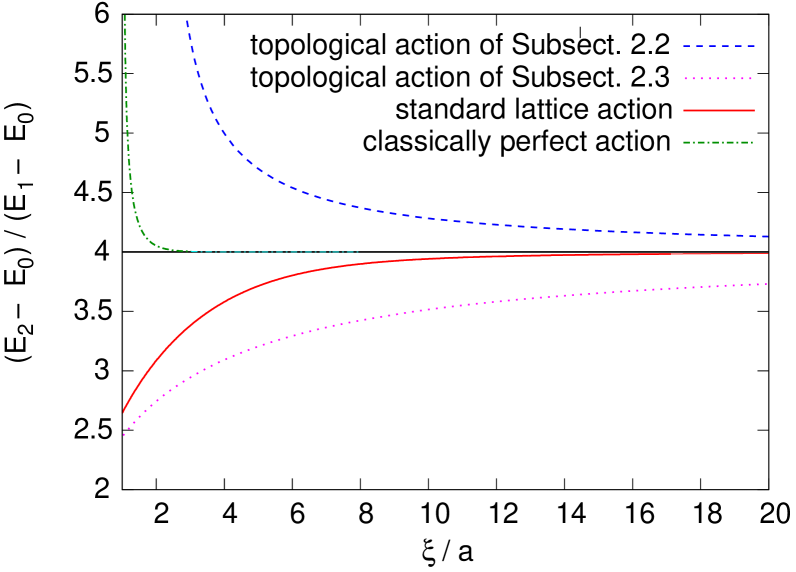
Figure 1: The scaling behavior of the ratio $(E_{2}-E_{0})/(E_{1}-E_{0})$ of energy gaps for different lattice actions: standard action (solid curve), topological action with (dotted curve), and without topological charge suppression (dashed curve), as well as classically perfect action (dashed-dotted curve). The topological lattice actions suffer from cut-off effects of ${\cal O}(a)$, while the standard action has only ${\cal O}(a^{2})$ artifacts. For the classically perfect action, the lattice artifacts are even exponentially suppressed. In the continuum $(E_{2}-E_{0})/(E_{1}-E_{0})=4$.

Indeed, one sees that the results obtained with the topological lattice action converge much slower than the ones for the standard or the classically perfect action. Still, as pointed out before, the topological lattice action has the correct quantum continuum limit.

Since the information about the topological charge distribution is encoded in the $\theta$-dependence of the energy spectrum $E_{m}(\theta)$, the topological susceptibility $\chi_{t}$ as well as other related topological quantities will also automatically come out correctly. In order to show this explicitly, let us also consider the partition function of the lattice model

$$Z(\theta)=\mbox{Tr}\ T(\theta)^{N}=\sum_{m\in{\mathbb{Z}}}\exp(-NaE_{m}(\theta))=\sum_{m\in{\mathbb{Z}}}\left[\frac{\sin((m-\theta/2\pi)\delta)}{(m-\theta/2\pi)\pi}\right]^{N},$$ (2.25)

such that

$$p(Q) = \frac{1}{2\pi}\int_{-\pi}^{\pi}d\theta\ Z(\theta)\exp(-i\theta Q)$$ (2.26)

$$= \frac{1}{2\pi}\int_{-\infty}^{\infty}d\theta\ \left[\frac{2\sin(\theta\delta/2\pi)}{\theta}\right]^{N}\exp(-i\theta Q).$$

Since $p(Q)$ is the Fourier transform of an $N$-th power, it is given by the $N$-fold convolution $p=p_{1}\star p_{1}\star\cdots\star p_{1}$. The elementary distribution is given by

$$p_{1}(Q)=\frac{1}{2\pi}\int_{-\infty}^{\infty}d\theta\ \frac{2\sin(\theta\delta/2\pi)}{\theta}\exp(-i\theta Q)=\Theta\left(Q+\frac{\delta}{2\pi}\right)-\Theta\left(Q-\frac{\delta}{2\pi}\right).$$ (2.27)

In this case, $Q\in{\mathbb{R}}$ is not restricted to integer values, because the elementary contributions to the total topological charge originate from local regions with open boundary conditions. We define the step function as $\Theta(Q)=1$ for $Q>0$, and as $\Theta(Q)=0$ otherwise. In the zero-temperature limit $\beta\rightarrow\infty$, the topological susceptibility now takes the form

$$\chi_{t}=\frac{\int_{-\infty}^{\infty}dQ\ p_{1}(Q)Q^{2}}{a\int_{-\infty}^{\infty}dQ\ p_{1}(Q)}=\frac{\int_{-\delta/2\pi}^{\delta/2\pi}dQ\ Q^{2}}{a\int_{-\delta/2\pi}^{\delta/2\pi}dQ}=\frac{1}{4\pi^{2}}\frac{\delta^{2}}{3a}=\frac{1}{4\pi^{2}I},$$ (2.28)

which is indeed the correct result of eq.(2.9) for the 1-d $O(2)$ model in the continuum.

It is interesting to note that this lattice action violates the inequality (2.13). This is obvious, because all allowed configurations have zero action. Still, for a given value of $\delta$ and for a given inverse temperature $\beta=Na$, the allowed topological charges are restricted to

$$|Q[\varphi]|\leq\frac{\delta}{2\pi}N=\frac{\delta\beta}{2\pi a},$$ (2.29)

such that

$$\frac{2\pi^{2}IQ[\varphi]^{2}}{\beta}\leq\frac{\pi I\delta^{2}\beta}{2a^{2}}=\frac{3\pi\beta}{2a}\rightarrow\infty.$$ (2.30)

Hence, unlike in the continuum theory, topologically non-trivial field configurations are not suppressed by the lattice action in the continuum limit $a\rightarrow 0$. Remarkably, nevertheless the lattice theory has the correct quantum continuum limit.

As a further scaling test, we compare the cut-off effects of the topological susceptibility in units of the mass gap, i.e. $\chi_{t}\xi$, for the various lattice actions. For the standard action one obtains

$$\chi_{t}^{s}\ \xi_{s}=\frac{1}{2\pi^{2}}\left(1+\frac{a^{2}}{3{\xi_{s}}^{2}}+\frac{a^{3}}{{\xi_{s}}^{3}}+\dots\right).$$ (2.31)

while for the classically perfect action one finds

$$\chi_{t}^{c}\ \xi_{c}=\frac{1}{2\pi^{2}}\left(1-\sqrt{\frac{\pi\xi_{c}}{a}}\left[1-\frac{4}{\pi^{2}}\right]\exp\left(-\frac{\pi^{2}\xi_{c}}{4a}\right)+\dots\right).$$ (2.32)

For the topological action, on the other hand, we obtain

$$\chi_{t}\xi=\frac{1}{4\pi^{2}}\frac{\delta^{2}}{3}\left[\log\frac{\delta}{\sin\delta}\right]^{-1}=\frac{1}{2\pi^{2}}\left(1-\frac{a}{5\xi}+\dots\right).$$ (2.33)

As before the lattice artifacts of the topological action are of ${\cal O}(a)$, while they are of ${\cal O}(a^{2})$ for the standard action and exponentially suppressed for the classically perfect action. The results for the various actions are illustrated in Figure 2.

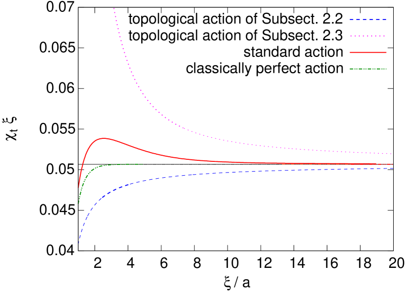
Figure 2: The scaling behavior of the product $\chi_{t}\xi$ of the topological susceptibility and the correlation length for different lattice actions: standard action (solid curve), topological action with (dotted curve) and without topological charge suppression (dashed curve), as well as classically perfect action (dashed-dotted curve). The topological lattice actions suffer from cut-off effects of ${\cal O}(a)$, while the standard action has only ${\cal O}(a^{2})$ artifacts. For the classically perfect action, the lattice artifacts are exponentially suppressed. The continuum value amounts to $\chi_{t}\xi=1/(2\pi^{2})$.

2.3 A Topological Lattice Action with Topological Charge Suppression

Let us now consider a topological lattice action which receives local contributions from the topological charge density, i.e.

$$S[\varphi]=\lambda\sum_{t}|(\varphi_{t+a}-\varphi_{t})\ \mbox{mod}\ 2\pi|.$$ (2.34)

A (dimensionless) coupling constant $\lambda>0$ suppresses configurations with non-zero topological charge. In particular, by construction this action obeys the inequality

$$S[\varphi]\geq 2\pi\lambda|Q[\varphi]|,$$ (2.35)

which is inconsistent with the corresponding inequality (2.13) of the continuum theory.

In this case, the transfer matrix takes the form

$$\langle\varphi_{t}|T(\theta)|\varphi_{t+a}\rangle=\exp(-\lambda|(\varphi_{t+a}-\varphi_{t})\ \mbox{mod}\ 2\pi|)\exp\left(-i\frac{\theta}{2\pi}(\varphi_{t+a}-\varphi_{t})\ \mbox{mod}\ 2\pi\right).$$ (2.36)

It is again diagonalized in the basis of angular momentum eigenstates and the corresponding eigenvalues are given by

$$\exp(-aE_{m}(\theta)) = \frac{1}{2\pi}\int_{-\pi}^{\pi}d\varphi\exp(-\lambda|\varphi|)\exp\left(i\left(m-\frac{\theta}{2\pi}\right)\varphi\right)$$ (2.37)

$$= \frac{1}{\pi}\frac{1}{\lambda^{2}+(m-\theta/2\pi)^{2}}\Big{\{}\lambda-\exp(-\pi\lambda)$$

$$\times \left[\lambda\cos\left(m\pi-\frac{\theta}{2}\right)-\left(m-\frac{\theta}{2\pi}\right)\sin\left(m\pi-\frac{\theta}{2}\right)\right]\Big{\}}.$$

For large $\lambda$, i.e. in the continuum limit, one then obtains

$$E_{m}(\theta)-E_{0}(0)=\frac{1}{a}\log\left[1+\frac{1}{\lambda^{2}}\left(m-\frac{\theta}{2\pi}\right)^{2}\right]\ \rightarrow\ \frac{1}{a\lambda^{2}}\left(m-\frac{\theta}{2\pi}\right)^{2}.$$ (2.38)

In order to match the continuum result of eq.(2.5), we thus identify

$$I=\frac{a\lambda^{2}}{2}\ \Rightarrow\ \lambda=\sqrt{\frac{2I}{a}}.$$ (2.39)

Using the inequality (2.35), one then concludes that the action of topologically non-trivial field configurations diverges in the continuum limit,

$$S[\varphi]\geq 2\pi\lambda|Q[\varphi]|=2\pi\sqrt{\frac{2I}{a}}|Q[\varphi]|\ \rightarrow\ \infty.$$ (2.40)

Remarkably, despite this fact, in the quantum continuum limit the $\theta$-dependent energy spectrum still agrees with the one of the continuum theory.

As before, we consider the lattice artifacts of the ratio of energy gaps, which now takes the form

$$\frac{E_{2}(0)-E_{0}(0)}{E_{1}(0)-E_{0}(0)}=4\left(1-\frac{3a}{2\xi}+\dots\right).$$ (2.41)

Again, the lattice artifacts, which are also illustrated in Figure 1, are of ${\cal O}(a)$. The artifacts of the topological lattice action with topological charge suppression are even a factor $5/2$ larger than for the topological action without topological charge suppression. In particular, even for $\xi=15a$ the deviations from the continuum limit are as large as 10 percent, while they are only about 0.5 percent with the standard action.

Let us again consider the $\theta$-dependent partition function

$$Z(\theta) = \mbox{Tr}\ T(\theta)^{N}=\sum_{m\in{\mathbb{Z}}}\exp(-NaE_{m}(\theta))=$$ (2.42)

$$= \sum_{m\in{\mathbb{Z}}}\left\{\frac{1}{\pi}\frac{1}{\lambda^{2}+(m-\theta/2\pi)^{2}}\{\lambda-\exp(-\pi\lambda)\right.$$

$$\times \left.\left[\lambda\cos\left(m\pi-\frac{\theta}{2}\right)-\left(m-\frac{\theta}{2\pi}\right)\sin\left(m\pi-\frac{\theta}{2}\right)\right]\}\right\}^{N}.$$

As before, the corresponding topological charge distribution $p(Q)$ is obtained as the $N$-fold convolution of an elementary distribution

$$p_{1}(Q) = \int_{-\infty}^{\infty}d\theta\ \frac{2}{(2\pi\lambda)^{2}+\theta^{2}}\left\{\lambda-\exp(-\pi\lambda)\left[\lambda\cos\frac{\theta}{2}-\frac{\theta}{\pi}\sin\frac{\theta}{2}\right]\right\}\exp(-i\theta Q)$$ (2.43)

$$= [1-\exp(-2\pi\lambda)]\exp(-2\pi\lambda|Q|).$$

The topological susceptibility in the zero-temperature limit is then given by

$$\chi_{t}=\frac{\int_{-\infty}^{\infty}dQ\ p_{1}(Q)Q^{2}}{a\int_{-\infty}^{\infty}dQ\ p_{1}(Q)}=\frac{1}{2\pi^{2}\lambda^{2}a}=\frac{1}{4\pi^{2}I},$$ (2.44)

which again is the correct quantum continuum limit.

Let us again consider the lattice artifacts of the product $\chi_{t}\xi$. Up to exponentially small corrections, we obtain

$$\chi_{t}\xi=\frac{1}{2\pi^{2}\lambda^{2}}\left[\log\left(1+\frac{1}{\lambda^{2}}\right)\right]^{-1}=\frac{1}{2\pi^{2}}\left(1+\frac{a}{2\xi}+\dots\right).$$ (2.45)

As for the topological action of the previous subsection, the lattice artifacts are of ${\cal O}(a)$. This result is also illustrated in Figure 2.

We hence conclude that, despite the fact that the two topological lattice actions do not have the correct classical continuum limit, cannot be treated perturbatively, or violate the classical inequality (2.13), they both have the correct quantum continuum limit. In particular, this holds for the $\theta$-dependent energy spectrum and all quantities derived from it, including the topological susceptibility.

3 The 1-d $O(3)$ Model

In this section we consider an angle-constraint topological lattice action for the 1-d $O(3)$ model, which describes a quantum mechanical particle moving on the surface of a sphere $S^{2}$. Again, despite the fact that the topological lattice action does not obey the correct classical continuum limit, it correctly reproduces the quantum continuum limit.

3.1 A Particle Moving on $S^{2}$

Let us now consider a particle of mass $M$ moving on a sphere $S^{2}$ of radius $R$. The Hamiltonian then takes the form

$$H=\frac{{\vec{L}}^{2}}{2I},$$ (3.1)

where $\vec{L}$ is the angular momentum and $I=MR^{2}$ is the moment of inertia. The corresponding eigenfunctions are the spherical harmonics $\langle\theta,\varphi|lm\rangle=Y_{lm}(\theta,\varphi)$ with $l\in\{0,1,2,\dots\}$ and $m\in\{-l,-l+1,\dots,l\}$, and the $(2l+1)$-fold degenerate energy eigenvalues are

$$E_{l}=\frac{l(l+1)}{2I}.$$ (3.2)

In this case, one cannot construct a topological charge and the Euclidean action is simply given by

$$S[\vec{e}]=\int dt\ \frac{I}{2}\partial_{t}\vec{e}\cdot\partial_{t}\vec{e},$$ (3.3)

with $\vec{e}(t)=(\sin\theta(t)\cos\varphi(t),\sin\theta(t)\sin\varphi(t),\cos\theta(t))$.

3.2 The 1-d $O(3)$ Model with a Topological Lattice Action

Let us now consider the $O(3)$ model with spins $\vec{e}_{t}=(\sin\theta_{t}\cos\varphi_{t},\sin\theta_{t}\sin\varphi_{t},\cos\theta_{t})$ attached to the sites $t$ of a 1-d lattice with spacing $a$. The lattice action constrains the angle between neighboring spins $\vec{e}_{t}$ and $\vec{e}_{t+a}$ to a maximal value $\delta$, i.e. $\vec{e}_{t}\cdot\vec{e}_{t+a}\geq\cos\delta$. The action vanishes as long as this constraint is satisfied and is infinite otherwise. The corresponding transfer matrix is then given by $\langle\theta_{t},\varphi_{t}|T|\theta_{t+a},\varphi_{t+a}\rangle=1$ for $\vec{e}_{t}\cdot\vec{e}_{t+a}\geq\cos\delta$, and $\langle\theta_{t},\varphi_{t}|T|\theta_{t+a},\varphi_{t+a}\rangle=0$ otherwise. We now put $\vec{e}_{t}=(0,0,1)$ and $\vec{e}_{t+a}=(\sin\theta\cos\varphi,\sin\theta\sin\varphi,\cos\theta)$. Inserting complete sets of states $|lm\rangle$ and using the fact that the transfer matrix is $O(3)$-invariant, i.e.

$$\langle lm|T|l^{\prime}m^{\prime}\rangle=\delta_{ll^{\prime}}\delta_{mm^{\prime}}\exp(-aE_{l}),$$ (3.4)

one obtains

$$\Theta(\cos\theta-\cos\delta) = \langle 0,0|T|\theta,\varphi\rangle=\sum_{l,m}\langle 0,0|lm\rangle\langle lm|T|lm\rangle\langle lm|\theta,\varphi\rangle$$ (3.5)

$$= \sum_{l,m}Y_{lm}(0,0)\exp(-aE_{l})Y_{lm}(\theta,\varphi)^{*}.$$

Inverting this relation, we find

$$Y_{lm}(0,0)\exp(-aE_{l}) = \int_{-1}^{1}d\cos\theta\int_{0}^{2\pi}d\varphi\ \Theta(\cos\theta-\cos\delta)Y_{lm}(\theta,\varphi)$$ (3.6)

$$= 2\pi\delta_{m,0}\int_{\cos\delta}^{1}dx\ \sqrt{\frac{2l+1}{4\pi}}P_{l}(x),$$

where $P_{l}(x)$ is a Legendre polynomial. Using $Y_{lm}(0,0)=\delta_{m,0}\sqrt{(2l+1)/4\pi}$ and applying the Legendre differential equation (with $P_{l}^{\prime}(x)=dP_{l}(x)/dx$)

$$\frac{d}{dx}\left[(1-x^{2})P_{l}^{\prime}(x)\right]+l(l+1)P_{l}(x)=0,$$ (3.7)

for $l\neq 0$ one obtains

$$\exp(-aE_{l}) = 2\pi\int_{\cos\delta}^{1}dx\ P_{l}(x)=-\frac{2\pi}{l(l+1)}(1-x^{2})P_{l}^{\prime}(x)|_{\cos\delta}^{1}$$ (3.8)

$$= \frac{2\pi}{l(l+1)}\sin^{2}\delta\ P_{l}^{\prime}(\cos\delta).$$

Similarly, for $l=0$ one finds $\exp(-aE_{0})=2\pi(1-\cos\delta)$, which results in

$$E_{l}-E_{0}=-\frac{1}{a}\log\left[\frac{1+\cos\delta}{l(l+1)}\ P_{l}^{\prime}(\cos\delta)\right].$$ (3.9)

Expanding in small values of $\delta$, i.e. putting $\cos\delta\approx 1-\delta^{2}/2$, one obtains

$$E_{l}-E_{0} = -\frac{1}{a}\log\left[\frac{2-\delta^{2}/2}{l(l+1)}\ P_{l}^{\prime}(1-\delta^{2}/2)\right]$$ (3.10)

$$= -\frac{1}{a}\log\left\{\frac{2}{l(l+1)}\left[P_{l}^{\prime}(1)-\frac{\delta^{2}}{4}\left[P_{l}^{\prime}(1)+2P_{l}^{\prime\prime}(1)\right]\right]\right\}+{\cal O}(\delta^{4})$$

$$= \frac{\delta^{2}}{8a}l(l+1)+{\cal O}(\delta^{4}).$$

Here we have used

$$P_{l}^{\prime}(1)=\frac{l(l+1)}{2},\ P_{l}^{\prime}(1)+2P_{l}^{\prime\prime}(1)=\left(\frac{l(l+1)}{2}\right)^{2}.$$ (3.11)

Hence, identifying

$$I=\frac{4a}{\delta^{2}},$$ (3.12)

we indeed reproduce the correct spectrum of eq.(3.2) in the quantum continuum limit. It turns out that in the 1-d $O(N)$ model the moment of inertia is given by $I=(N+1)a/\delta^{2}$.

Let us again consider the lattice artifacts in the ratio of energy gaps, which now takes the form

$$\frac{E_{2}(0)-E_{0}(0)}{E_{1}(0)-E_{0}(0)}=3\left(1+\frac{a}{3\xi}+\dots\right).$$ (3.13)

As for the 1-d $O(2)$ model, the lattice artifacts are of ${\cal O}(a)$.

4 The 2-d $O(3)$ Model

In this section we consider the 2-d $O(3)$ model using numerical simulations. We first summarize the results obtained before in the continuum and with standard as well as modified lattice actions. In analogy to Subsections 2.2 and 2.3 we then investigate two topological lattice actions, one that does and one that does not obey a Schwarz inequality between action and topological charge. Remarkably, in both cases we will again obtain the correct quantum continuum limit. While it is well-known that in this model the topological susceptibility is logarithmically divergent, we will see that the correlator of the topological charge density has a finite continuum limit. Hence there are topological quantities that do have a finite continuum limit in this model.

4.1 The 2-d $O(3)$ Model in the Continuum and with the Standard Lattice Action

In this subsection we summarize results obtained before either in the continuum or using the standard lattice action for the 2-d $O(3)$ model. In the continuum, the 2-d $O(3)$ model has the Euclidean action

$$S[\vec{e}]=\frac{1}{2g^{2}}\int d^{2}x\ \partial_{\mu}\vec{e}\cdot\partial_{\mu}\vec{e}-i\theta Q[\vec{e}].$$ (4.1)

Here $\vec{e}(x)\in S^{2}$ is a 3-component unit-vector field defined at each point $x$ in a 2-dimensional Euclidean space-time, and the topological charge is given by

$$Q[\vec{e}]=\frac{1}{8\pi}\int d^{2}x\ \varepsilon_{\mu\nu}\vec{e}\cdot(\partial_{\mu}\vec{e}\times\partial_{\nu}\vec{e})\in\Pi_{2}[S^{2}]={\mathbb{Z}}.$$ (4.2)

It is straightforward to show that the following integral, which is non-negative by construction, takes the form

$$I=\int d^{2}x\ (\partial_{\mu}\vec{e}\pm\varepsilon_{\mu\nu}\vec{e}\times\partial_{\nu}\vec{e})^{2}=4g^{2}S[\vec{e}]\pm 16\pi Q[\vec{e}]\geq 0.$$ (4.3)

This immediately implies the Schwarz inequality

$$S[\vec{e}]\geq\frac{4\pi}{g^{2}}|Q[\vec{e}]|.$$ (4.4)

Field configurations which saturate this inequality are (anti-)self-dual, i.e.

$$\partial_{\mu}\vec{e}=\pm\varepsilon_{\mu\nu}\vec{e}\times\partial_{\nu}\vec{e},$$ (4.5)

and are known as (anti-)instantons. For these configurations the Lagrangian ${\cal L}(\vec{e})$ (at $\theta=0$) is proportional to the absolute value of the topological charge density $q(\vec{e})$, i.e.

$${\cal L}(\vec{e})=\frac{1}{2g^{2}}\partial_{\mu}\vec{e}\cdot\partial_{\mu}\vec{e}=\frac{1}{2g^{2}}\big{|}\varepsilon_{\mu\nu}\vec{e}\cdot(\partial_{\mu}\vec{e}\times\partial_{\nu}\vec{e})\big{|}=\frac{4\pi}{g^{2}}|q(\vec{e})|.$$ (4.6)

In Section 4.3 we will introduce a topological lattice action such that ${\cal L}(\vec{e})$ is proportional to $|q(\vec{e})|$ for all configurations, not just for instantons or anti-instantons.

Remarkably, at $\theta=0$ the 2-d $O(3)$ model can be solved exactly using the Bethe ansatz [53, 54, 55]. Based on these results, using the Wiener-Hopf technique, the exact mass gap of the 2-d $O(3)$ model

$$m=\frac{8}{e}\Lambda_{\overline{MS}},$$ (4.7)

has been derived [56]. Here $e$ is the base of the natural logarithm, and $\Lambda_{\overline{MS}}$ is the scale generated by dimensional transmutation in the modified minimal subtraction renormalization scheme. Even the finite-size effects of the mass gap $m(L)$ for the 2-d $O(3)$ model on a finite periodic spatial interval of size $L$ have been calculated analytically [57]. A dimensionless physical quantity

$$u_{0}=Lm(L)=L/\xi(L),$$ (4.8)

is then obtained as the ratio of the spatial size $L$ and the finite-volume correlation length $\xi(L)=1/m(L)$. Similarly, one defines the step scaling function (with scale factor 2)

$$\sigma(2,u_{0})=2Lm(2L),$$ (4.9)

which is thus also known analytically. Later, we will compare Monte Carlo data for $\sigma(2,u_{0})$, obtained with a topological lattice action, with the analytic result. The step scaling function was first studied on the lattice by Lüscher, Weisz, and Wolff [58] using the standard action

$$S[\vec{e}]=\frac{1}{g^{2}}\sum_{x,\mu}\vec{e}_{x}\cdot\vec{e}_{x+\hat{\mu}}.$$ (4.10)

Now $x$ denotes the lattice sites, and $\hat{\mu}$ is a vector of length $a$ pointing in the $\mu$-direction. The step scaling function is affected by lattice artifacts which — for some time — seemed not to be described by Symanzik’s effective theory. Interestingly, a recent careful study of the lattice artifacts has shown that large logarithms arise, and that Symanzik’s theory does describe the lattice artifacts correctly [59, 60]. Hence, one may conclude that the continuum limit of the finite-volume mass gap $m(L)$ is finally well understood. Furthermore, excellent agreement between the Zamolodchikov bootstrap S-matrix and Monte Carlo data, obtained with both the standard and a classically perfect lattice action, has been reported [61].

Let us now discuss the topological susceptibility

$$\chi_{t}=\frac{\langle Q^{2}\rangle}{V}$$ (4.11)

of the 2-d $O(3)$ model. Here $V=\beta L$ is the space-time volume. Based on naive dimensional analysis, one would expect that $\chi_{t}\xi^{2}$ approaches a constant in the continuum limit. While this expectation is met in 2-d ${\mathbb{C}P}(N-1)$ models with $N\geq 3$, the ${\mathbb{C}P}(1)$ (or equivalently $O(3)$) model behaves differently. The pathological behavior of $\chi_{t}$ in the 2-d $O(3)$ model manifests itself already in the continuum formulation. As was pointed out by Lüscher [29], the integration over the instanton size parameter $\rho$ in a semi-classical calculation gives rise to a logarithmically divergent ultra-violet contribution to $\chi_{t}$ which is proportional to $\int d\rho/\rho$.

Berg and Lüscher have investigated $\chi_{t}$ using a geometric definition of the lattice topological charge [28]. In this definition, each plaquette of the square lattice is divided into two triangles, as illustrated in Figure 3.

Figure 3: Decomposition of the square lattice into triangles to be used to define the action and the topological charge.

The spins $\vec{e}_{1}$, $\vec{e}_{2}$, and $\vec{e}_{3}$ at the three corners of a lattice triangle $t_{123}$ define the corners of a spherical triangle on $S^{2}$. The oriented area $A_{123}$ of the spherical triangle is given by

$$A_{123}=2\varphi\in[-2\pi,2\pi],\quad X+iY=r\exp(i\varphi),$$

$$X=1+\vec{e}_{1}\cdot\vec{e}_{2}+\vec{e}_{2}\cdot\vec{e}_{3}+\vec{e}_{3}\cdot\vec{e}_{1},\quad Y=\vec{e}_{1}\cdot(\vec{e}_{2}\times\vec{e}_{3}).$$ (4.12)

The geometric topological charge is the sum of the oriented areas $A_{xyz}$ over all triangles $t_{xyz}$, normalized by the area $4\pi$ of $S^{2}$, i.e.

$$Q[\vec{e}]=\frac{1}{4\pi}\sum_{t_{xyz}}A_{xyz}\in{\mathbb{Z}}.$$ (4.13)

The decomposition of the square lattice into triangles illustrated in Figure 3 is invariant under $\pi/2$ rotations and translation invariant by an even number of lattice spacings. Obviously, the topological charge inherits these symmetries.

Figure 4: A given plaquette 1234 can be decomposed into two triangles in two alternative ways: a) 123 and 243 or b) 124 and 143.

As illustrated in Figure 4, an individual lattice plaquette 1234 can be divided into two triangles 123 and 243 or alternatively into triangles 124 and 143. In general, it is not guaranteed that $A_{123}+A_{243}$ is equal to $A_{124}+A_{143}$. However, if the relative angle between nearest-neighbor spins is smaller than $\pi/2$, one can indeed show that $A_{123}+A_{243}=A_{124}+A_{143}$. In that case, the topological charge becomes independent of the particular decomposition into triangles, and thus becomes invariant even against translations by a single lattice spacing. Here we prefer to work on a triangulated quadratic (rather than a triangular) lattice because the definition of the step scaling function refers to a rectangular space-time volume.

The geometric topological charge is undefined for a set of exceptional field configurations, which form a set of measure zero in configuration space. These exceptional configurations contain a spherical triangle that covers exactly one half of $S^{2}$ and thus has an area $\pm 2\pi$. The infinitesimal neighborhood of an exceptional configuration contains configurations whose topological charges differ by 1. If the relative angle between nearest-neighbor spins is smaller than $\pi/2$, exceptional configurations cannot arise. When one uses the standard lattice action, exceptional configurations have a finite action. In the following subsection, we will consider a topological lattice action that constrains the relative angle between nearest-neighbor spins to a maximum value $\delta$. When $\delta<\pi/2$, exceptional configurations are excluded, and — just as in the continuum — different topological sectors are then separated by infinite-action barriers. This means that the angle-constraint topological action, but not the standard action, naturally leads to a unique segmentation of configuration space into distinct topological sectors.

In addition to the logarithmic ultra-violet divergence that is present in the continuum theory, in the 2-d lattice $O(3)$ model $\chi_{t}$ is affected by additional short-distance artifacts. These so-called dislocations are minimal action field configurations with a non-zero topological charge. As such, they depend on both the definition of the lattice action and the definition of the lattice topological charge. Using the standard lattice action in combination with the geometric definition of the lattice topological charge, the dislocations are exceptional configurations with an action $S_{d}=c/g^{2}$ with $c\approx 6.69<4\pi$ [29]. Semi-classical arguments (which, however, are not rigorous) suggest that the topological susceptibility should scale as $\chi_{t}\propto\exp(-S_{d})$. Due to asymptotic freedom, the correlation length scales as $\xi/a\propto\exp(2\pi/g^{2})$, where $2\pi$ is the universal 1-loop coefficient of the $\beta$-function. Hence, one expects a power-law divergence of the dimensionless combination

$$\chi_{t}\xi^{2}\propto\exp(-S_{d})\exp\left(\frac{4\pi}{g^{2}}\right)=\exp\left(\frac{4\pi-c}{g^{2}}\right)\propto\left(\frac{\xi}{a}\right)^{2-c/2\pi}.$$ (4.14)

Dislocations have been eliminated in [33] by using a classically perfect lattice action in combination with a classically perfect definition of the lattice topological charge. Perfect discretizations are based on the renormalization group and eliminate cut-off effects at the classical level. In particular, one then has $S_{d}=4\pi/g^{2}$, i.e. $c=4\pi$. Interestingly, the topological susceptibility was then found to still diverge logarithmically. From all this one concludes that $\chi_{t}$ does not have a finite continuum limit in the 2-d $O(3)$ model.

The situation is different in 2-d ${\mathbb{C}P}(N-1)$ models with $N\geq 3$. While $\chi_{t}$ is still divergent in the ${\mathbb{C}P}(2)$ model when one uses the standard lattice action in combination with the geometric definition of the topological charge, dislocations can be suppressed by choosing a modified lattice action [29, 32]. For $N\geq 4$, dislocations do not cause any problems, even when the standard action is used. Similarly, in 4-d $SU(N)$ lattice Yang-Mills theories, when one uses the geometric topological charge, $\chi_{t}$ suffers from dislocations for $N=2$ and 3, which again can be suppressed by using a modified lattice action [37, 38].

4.2 A Topological Lattice Action without Topological Charge Suppression

In analogy to the 1-d $O(2)$ and $O(3)$ models, we now investigate the 2-d $O(3)$ model with a topological lattice action that constrains the relative angle of nearest-neighbor spins on a square lattice to a maximum angle $\delta$. All configurations that violate this constraint are forbidden and thus have infinite action, while all other configurations are allowed and have zero action. This action can be simulated with the very efficient Wolff cluster algorithm [62, 63]. Two neighboring spins are put in the same cluster if flipping one of them on a randomly chosen reflection plane would increase their relative angle beyond $\delta$. For the efficiency of the algorithm it is essential that, using this method, only spins on the same side of the reflection plane end up in the same cluster. The correlation function of two spins $\langle\vec{e}_{x}\cdot\vec{e}_{y}\rangle$ can then be computed very accurately using an improved estimator.

We have fine-tuned the maximal angle $\delta$ such that the finite-volume mass gap $m(L)$ satisfies $u_{0}=Lm(L)=1.0595$ for lattices with $L/a=10,16,32$, and 64. The corresponding values of $\delta$ are listed in Table 1.

$L/a$	$\delta/\pi$	$\xi(L)/a$	$\xi(2L)/a$
10	0.44858728	9.4383(1)	15.9515(15)
16	0.434009	15.1013(2)	25.4787(10)
32	0.415095	30.2029(2)	50.847(3)
64	0.398665	60.406(1)	101.578(4)

Table 1: Constraint angle $\delta$ that leads to $u_{0}=Lm(L)=1.0595$ for various lattice sizes together with the correlation lengths $\xi(L)$ and $\xi(2L)$.

By measuring the mass gap $m(2L)$ for these values, we have then determined the lattice value $\Sigma(2,u_{0},a/L)=2Lm(2L)$ of the step scaling function, which is known to approach the continuum limit $\sigma(2,u_{0}=1.0595)=1.26121035(2)$ [59, 60].

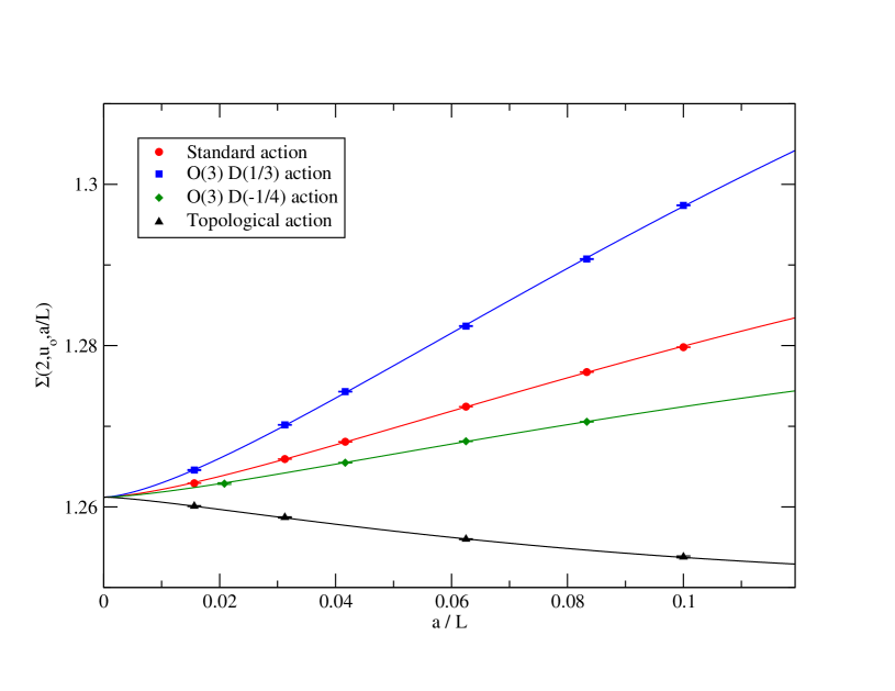
Figure 5: Cut-off dependence of the step scaling function $\Sigma(2,u_{0},a/L)$ at $u_{0}=1.0595$ for four different lattice actions: the standard as well as two different modified actions ($O(3)D(1/3)$ and $O(3)D(-1/4)$) [59], and the topological lattice action without topological charge suppression. The lines are fits based on Symanzik’s effective theory with the continuum value fixed to the exact result $\Sigma(2,u_{0}=1.0595,a/L\rightarrow 0)=\sigma(2,u_{0}=1.0595)=1.26121035(2)$.

Figure 5 compares the cut-off effects of $\Sigma(2,u_{0},a/L)$ for the topological action with the standard and with two modified actions. At first glance, it seems that all four actions have lattice artifacts of ${\cal O}(a)$. This would contradict Symanzik’s effective theory. However, as investigated in detail [59, 60], the standard and the modified actions indeed have lattice artifacts of ${\cal O}(a^{2}\log^{3}(a/L))$, with large logarithmic corrections mimicking ${\cal O}(a)$ effects. In particular, Symanzik’s theory correctly describes the observed lattice artifacts. Since lattice perturbation theory is not applicable to topological lattice actions, one might think that one cannot use Symanzik’s theory to predict the lattice artifacts. However, this is true only to some extent. Symanzik’s effective theory is formulated in the continuum and should be applicable to any lattice theory that reaches the correct quantum continuum limit. As we have seen analytically for the 1-d $O(2)$ and $O(3)$ models, the topological lattice actions suffer from lattice artifacts of ${\cal O}(a)$, which would contradict Symanzik’s effective theory. However, since the underlying power-counting does not work in quantum mechanics, Symanzik’s theory is not applicable in that case. In the 2-d case, however, Symanzik’s theory applies even to topological lattice actions. This suggests to fit the lattice step scaling function to

$$\Sigma(2,u_{0}=1.0595,a/L)=\sigma(2,u_{0}=1.0595)+\frac{a^{2}}{L^{2}}\left[B\log^{3}(L/a)+C\log^{2}(L/a)+\dots\right],$$ (4.15)

which gives a good fit for $B=-0.067(4)$ and $C=0.014(9)$. Interestingly, in the range considered here, the lattice artifacts of the topological action are smaller than those of the standard action, for which one obtains $B=0.041(6)$ and $C=0.26(2)$. In fact, for the standard action at $L/a=64$ the sub-leading term proportional to $\log^{2}(L/a)$ is still larger than the leading term proportional to $\log^{3}(L/a)$, while this is not the case for the topological action. One can estimate that the lattice artifacts of the standard action will be smaller than the ones of the topological action only for correlation lengths larger than about $5\times 10^{4}a$. Furthermore, if one uses $\sigma(2,u_{0}=1.0595)$ as a fit parameter, only the topological action data are consistent with the exact value within error bars, while the other actions give rise to small deviations. Given the fact that the topological action violates the classical continuum limit, and is thus tree-level impaired, it performs remarkably well. This may perhaps encourage the use of topological lattice actions also in other models, including Abelian and non-Abelian gauge theories.

The very accurate approach to the exact continuum result for $\sigma(2,u_{0}=1.0595)$ strongly suggests that the topological lattice action indeed leads into the standard universality class of the 2-d $O(3)$ model. This confirms earlier results of [11, 13, 15, 14] and also justifies a posteriori the use of a topological lattice action in [17].

4.3 A Topological Lattice Action with Topological Charge Suppression

In analogy to the action for the 1-d $O(2)$ model discussed in Section 2.3, we now introduce a topological lattice action for the 2-d $O(3)$ model which explicitly suppresses topological charges and obeys a Schwarz inequality. Again, the action is given by the absolute value of the topological charge density, i.e.

$$S[\vec{e}]=\lambda\sum_{t_{xyz}}|A_{xyz}|.$$ (4.16)

Here $|A_{xyz}|$ is the area of the spherical triangle on $S^{2}$ defined by the spins $\vec{e}_{x}$, $\vec{e}_{y}$, and $\vec{e}_{z}$ at the three corners of a lattice triangle $t_{xyz}$, cf. eq.(4.1), and $\lambda$ is a positive coupling constant. By construction, this action obeys the inequality

$$S[\vec{e}]\geq\lambda\Big{|}\sum_{t_{xyz}}A_{xyz}\Big{|}=4\pi\lambda|Q[\vec{e}]|.$$ (4.17)

A comparison with the Schwarz inequality eq.(4.4) of the continuum theory may suggest to identify $\lambda=1/g^{2}$, but, as we will see, this is not necessarily justified. By construction, for this topological lattice action the Lagrangian ${\cal L}(\vec{e})$ is proportional to the absolute value of the topological charge density, i.e. ${\cal L}(\vec{e})=4\pi\lambda|q(\vec{e})|$, for all configurations. In the continuum theory the corresponding eq.(4.6) is satisfied only for instantons or anti-instantons. It is interesting to investigate the limit $\lambda\rightarrow\infty$. Then the allowed configurations only contain spherical triangles of zero area. Consequently, at $\lambda=\infty$ all spins $\vec{e}_{x}$ fall on a common great circle in $S^{2}$, and thus seem to represent an $O(2)$ model. When a triangle $t_{xyz}$ contains an $O(2)$ vortex, the corresponding area is $|A_{xyz}|=2\pi$. Hence, at $\lambda=\infty$, the 2-d $O(3)$ model from above reduces to a 2-d $O(2)$ model from which vortices have been eliminated. Such a model is expected to be in a massless phase. In the 2-d $O(3)$ model, the continuum limit is approached at $\lambda\rightarrow\infty$, not by putting $\lambda=\infty$. In particular, universality suggests that we should still recover the asymptotically free continuum limit of the 2-d $O(3)$ model.

Unfortunately, the action of eq.(4.16) cannot be simulated with an efficient Wolff-type embedding cluster algorithm. While it is possible to define a cluster algorithm that is ergodic and obeys detailed balance, one is forced to put spins in one common cluster although they are on different sides of the reflection plane. This renders the algorithm inefficient. Hence we have used a Metropolis algorithm to simulate this action. A high-precision study of the mass gap, as described in the previous subsection, is then not feasible. A numerically better accessible quantity is the second moment correlation length, which does not require a fit of the correlation function $G(x-y)=\langle\vec{e}_{x}\cdot\vec{e}_{y}\rangle$ at large distances. Instead one considers the Fourier transform

$$\widetilde{G}(p)=\sum_{x}G(x)\exp(ipx)$$ (4.18)

for a quadratic $L\times L$ lattice, which yields the susceptibility $\chi=\widetilde{G}(p=0)$ as well as the corresponding quantity at the smallest non-zero momentum $F=\widetilde{G}(p=(2\pi/L,0))$. The second moment correlation length is then defined as

$$\xi_{2}(L)=\left(\frac{\chi-F}{4F\sin^{2}(\pi/L)}\right)^{1/2}.$$ (4.19)

Using the corresponding mass $m_{2}(L)=1/\xi_{2}(L)$ one can define the step scaling function for the second moment correlation length as $\Sigma_{2}(2,m_{2}(L)L,a/L)=2Lm_{2}(2L)$. In the continuum limit, $\xi_{2}(L)/a\rightarrow\infty$, this function is again universal and has been determined in [65]. The universality has been verified in the $(2+1)$-d spin $1/2$ quantum Heisenberg model [66], which dimensionally reduces to the 2-d $O(3)$ model in the low-temperature limit [67]. We have measured the step scaling function $\Sigma_{2}(2,m_{2}(L)L,a/L)$ on quadratic lattices with $L/a=50$ and 100. In addition, we have measured this quantity for the topological lattice action of the previous subsection, which does not explicitly suppress topological charges. As illustrated in Figure 6, in both cases one finds very good agreement with the step scaling function obtained with the standard action. This again confirms that topological lattice actions lead to the correct quantum continuum limit, despite the fact that the classical continuum limit is not correctly represented.

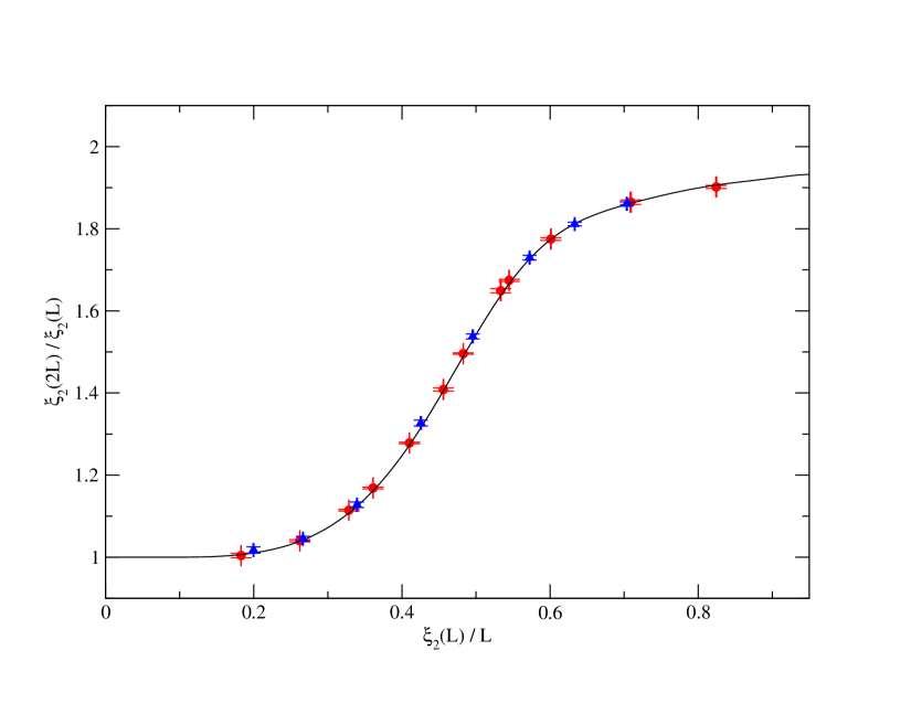
Figure 6: The ratio of second moment correlation lengths $\xi_{2}(2L)/\xi_{2}(L)$ obtained with the topological lattice action with (triangles) and without topological charge suppression (circles). Within error bars the data fall onto the universal curve that was extracted from simulations with the standard action [65].

4.4 Topological Susceptibility from Topological Lattice Actions

As discussed in the introduction, in the 2-d $O(3)$ model the topological susceptibility $\chi_{t}$ does not have a finite continuum limit. When the standard lattice action is used, based on (non-rigorous) semi-classical arguments one would expect a power-law divergence of $\chi_{t}$ due to dislocations which are short-range lattice artifacts carrying non-zero topological charge [29]. Even when a classically perfect action is used in combination with a classically perfect topological charge, $\chi_{t}$ still diverges logarithmically [33]. The logarithmic divergence is not a lattice artifact, but is an inherent feature of the 2-d $O(3)$ model even in the continuum. In this subsection we investigate the topological susceptibility using the two topological lattice actions with and without explicit topological charge suppression.

First, we consider the topological lattice action of Subsection 4.2 which does not explicitly suppress topological charges and which violates the Schwarz inequality. In order to hold the physical volume fixed while approaching the continuum limit, we demand $L=4\xi_{2}(L)$. Since it is easier to compute numerically, we base this criterion on the second moment correlation length $\xi_{2}(L)$, and not on the inverse mass gap $\xi(L)$, which is consistently just about 1.7 percent larger than $\xi_{2}(L)$. In the infinite volume limit the ratio $\xi/\xi_{2}=1.0007(1)$ has been determined very accurately in [64]. As illustrated in Figure 7, the discrepancy between this result and the ratio $\xi(L)/\xi_{2}(L)=1.017(3)$ observed at $L=4\xi_{2}(L)$ can be attributed to finite volume effects.

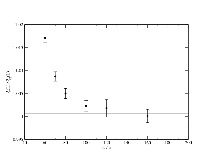
Figure 7: The ratio $\xi(L)/\xi_{2}(L)$ as a function of $L/a$ (at fixed $\delta/\pi=0.4849$) is consistent with the infinite volume result $\xi/\xi_{2}=1.0007(1)$ obtained in [64]. The infinite volume result is represented by the horizontal line.

Figure 8 shows the finite volume correlation length $\xi_{2}(L)/a$ as a function of the constraint angle $\delta$, together with a fit of the form

$$\frac{\xi_{2}(L)}{a}=Ag^{2}\exp\left(\frac{2\pi}{g^{2}}\right),\ \frac{1}{g^{2}}=\frac{b}{\delta^{2}}+c,$$ (4.20)

which yields $A=0.24(2)$, $b=0.263(2)$, and $c=-0.54(2)$, with $\chi^{2}/\mbox{d.o.f.}\approx 0.7$. Only the large lattices with $L/a\geq 200$ are included in the fit. The exponential increase of the correlation length is a consequence of asymptotic freedom. The fit assumes asymptotic scaling and contains the universal 1- and 2-loop coefficients of the $\beta$-function. The relation between $\delta$ and $g$ is inspired by the corresponding relation eq.(3.12) in the 1-d $O(3)$ model. It should, however, be pointed out that it is just a phenomenological ansatz which cannot be derived analytically, because perturbation theory does not apply to topological lattice actions. For the standard action, asymptotic scaling is known to set in only at very large correlation lengths [65]. Hence, also the value of $b$ determined here may not yet correspond to the asymptotic value in the continuum limit. Again, since perturbation theory is not applicable to topological lattice actions, one cannot determine the asymptotic value of $b$ analytically.

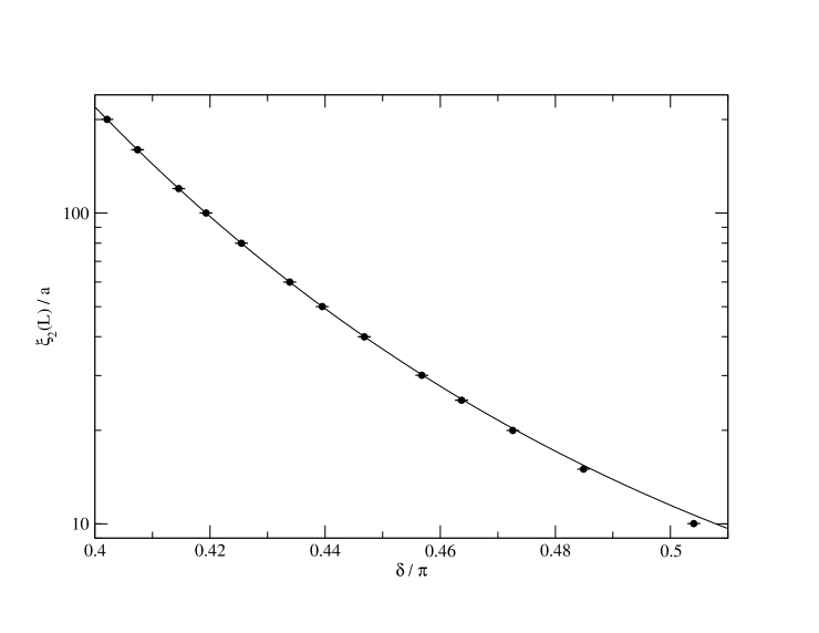
Figure 8: Second moment correlation length $\xi_{2}(L)/a$ at fixed physical size $L=4\xi_{2}(L)$ as a function of the constraint angle $\delta$. The line is a fit of the form of eq.(4.20), $\xi_{2}(L)/a=Ag^{2}\exp(2\pi/g^{2})$ with $1/g^{2}=b/\delta^{2}+c$.

In order to investigate the scaling of the topological susceptibility, we consider the dimensionless combination

$$16\chi_{t}(L)\xi_{2}(L)^{2}=16\frac{\langle Q^{2}\rangle(L)}{L^{2}}\left(\frac{L}{4}\right)^{2}=\langle Q^{2}\rangle(L),$$ (4.21)

as we approach the continuum limit $\xi_{2}(L)/a\rightarrow\infty$. In Table 2 we list the results of Monte Carlo simulations on various lattice sizes ranging from $L/a=40$ to $L/a=800$.

$L/a$	$\delta/\pi$	$\xi_{2}(L)/a$	$\xi(L)/a$	$\langle Q^{2}\rangle(L)$
40	0.50405	10.016(1)	10.20(2)	1.083(5)
60	0.48490	14.996(8)	15.29(4)	1.299(6)
80	0.47260	19.981(4)	20.34(6)	1.455(7)
100	0.46370	24.99(2)	25.46(8)	1.598(9)
120	0.45680	30.061(4)	30.57(8)	1.72(2)
160	0.44680	39.98(2)	40.67(9)	1.923(9)
200	0.43950	50.02(1)	50.75(9)	2.09(2)
240	0.43385	59.98(2)	60.97(9)	2.23(1)
320	0.42545	79.98(3)	81.18(9)	2.45(2)
400	0.41930	100.07(3)	101.5(2)	2.64(2)
480	0.41455	119.92(4)	121.8(3)	2.78(2)
640	0.40740	159.87(7)	162.5(3)	3.046(8)
800	0.40210	200.27(6)	203.7(3)	3.22(2)

Table 2: Monte Carlo data for the topological charge squared $\langle Q^{2}\rangle(L)$ at fixed physical size $L=4\xi_{2}(L)$ approaching the continuum limit $\xi_{2}(L)/a\rightarrow\infty$. Here $\xi_{2}(L)$ is the second moment correlation length, defined in eq.(4.19), while $\xi(L)$ is the inverse mass gap, and $\delta$ is the constraint angle in the topological action of Subsection 4.2.

Since this topological action vanishes for all allowed configurations, the dislocation action is $S_{d}=0$. Hence, based on a naive semi-classical argument, one might expect $\chi_{t}\xi^{2}\propto\exp(-S_{d})(\xi/a)^{2}=(\xi/a)^{2}$. Such a power-law divergence is not reflected by the numerical data depicted in Figure 9. Instead, the data are well fitted by

$$\langle Q^{2}\rangle(L)=A\log\left(\frac{L+L_{0}}{L_{1}}\right),$$ (4.22)

with $A=0.91(1)$, $L_{0}/a=39(2)$, $L_{1}/a=24(1)$, and $\chi^{2}/\mbox{d.o.f.}\approx 0.5$. A power-law fit $\langle Q^{2}\rangle(L)=BL^{\nu}+C$ yields a small power $\nu=0.21(2)$, and $\chi^{2}/\mbox{d.o.f.}\approx 1.9$.

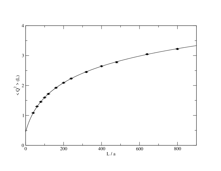
Figure 9: The topological charge squared $\langle Q^{2}\rangle(L)$ at fixed physical size $L=4\xi_{2}(L)$, for the topological lattice action of Subsection 4.2. As one approaches the continuum limit $\xi_{2}(L)/a\rightarrow\infty$, $\langle Q^{2}\rangle(L)$ diverges logarithmically. The line is a fit of the form of eq.(4.22), $\langle Q^{2}\rangle(L)=A\log((L+L_{0})/L_{1})$.

A logarithmic divergence of $\langle Q^{2}\rangle(L)$ was already encountered in the continuum theory [30] and was also observed on the lattice using a classically perfect action [33]. It is interesting that the same behavior arises for the topological action which should be most vulnerable by dislocations. While the naive semi-classical argument is not rigorous, it is still remarkable that even the presence of zero-action dislocations does not spoil the logarithmic divergence of the continuum theory. This suggests that dislocations may not cause power-law divergences in other cases, including 2-d ${\mathbb{C}P}(N-1)$ models and 4-d non-Abelian gauge theories, either. Indeed, no such divergence has been detected, for example, in numerical data for $\chi_{t}$ in 4-d $SU(2)$ Yang-Mills theory [68].

We have investigated $\langle Q^{2}\rangle(L)$ at fixed physical size $L=4\xi_{2}(L)$, also for the topological action of Subsection 4.3, which explicitly suppresses topological charges. The corresponding numerical results are listed in Table 3.

$L/a$	$4\pi\lambda$	$\xi_{2}(L)/a$	$\langle Q^{2}\rangle(L)$
40	11.9215	10.00(2)	1.102(2)
60	13.781	14.98(2)	1.282(2)
80	15.112	20.00(4)	1.419(3)
120	16.988	30.04(5)	1.631(3)
160	18.325	40.00(6)	1.784(4)

Table 3: Monte Carlo data for the topological charge squared $\langle Q^{2}\rangle(L)$ at fixed physical size $L=4\xi_{2}(L)$ approaching the continuum limit $\xi_{2}(L)/a\rightarrow\infty$. Here $\xi_{2}(L)$ is the second moment correlation length and $\lambda$ is the coupling constant in the topological action of Subsection 4.3.

Since in this case no efficient cluster algorithm is available, the calculation is limited to lattices up to $L/a=160$. As illustrated in Figure 10, the data for $\langle Q^{2}\rangle(L)$ are again consistent with the logarithmic divergence of eq.(4.22). Here the best fit yields $A=0.63(2)$, $L_{0}/a=20(3)$, $L_{1}/a=10(1)$, with $\chi^{2}/\mbox{d.o.f.}\approx 0.4$.

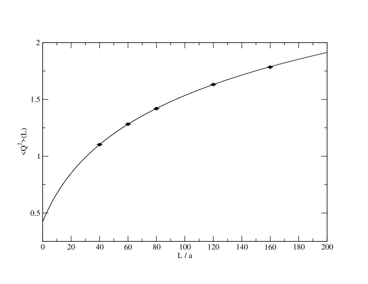
Figure 10: The topological charge squared $\langle Q^{2}\rangle(L)$ at fixed physical size $L=4\xi_{2}(L)$, for the topological lattice action of Subsection 4.3. The line is a fit of the form of eq.(4.22), $\langle Q^{2}\rangle(L)=A\log((L+L_{0})/L_{1})$.

In this case, we fit the second moment correlation length to the form

$$\frac{\xi_{2}(L)}{a}=Ag^{2}\exp\left(\frac{2\pi}{g^{2}}\right),\ \frac{1}{g^{2}}=b\lambda,$$ (4.23)

which yields $A=0.19(1)$, $b=0.045(1)$. The results are illustrated in Figure 11.

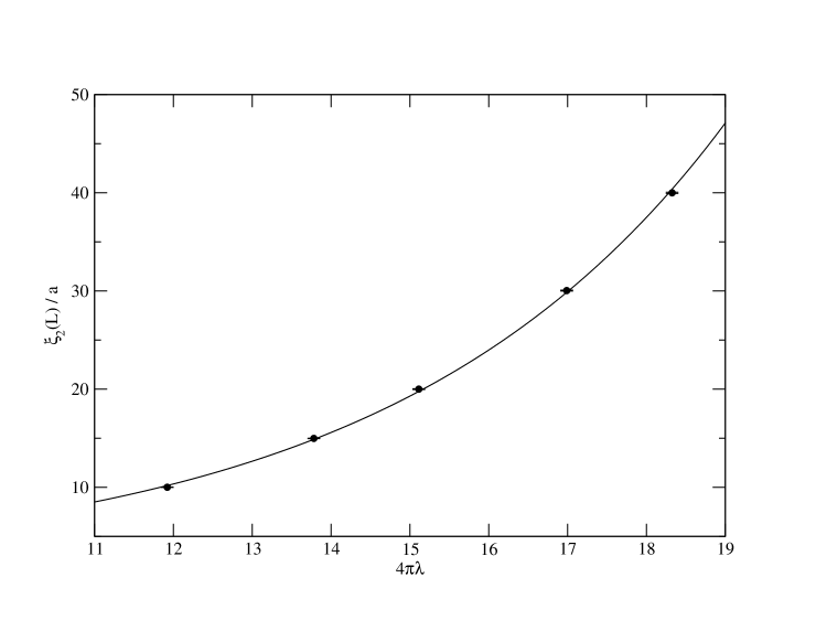
Figure 11: Second moment correlation length $\xi_{2}(L)/a$ at fixed physical size $L=4\xi_{2}(L)$ as a function of $4\pi\lambda$. The line is a fit of the form of eq.(4.23), $\xi_{2}(L)/a=Ag^{2}\exp(2\pi/g^{2})$ with $1/g^{2}=b\lambda$.

It should be pointed out that the relation between $\lambda$ and $g$ is again just an ansatz, which cannot be derived analytically, because perturbation theory is not applicable to topological lattice actions. Furthermore, one cannot be sure that the above value of $b$ persists in the continuum limit. The lattice Schwarz inequality (2.35), $S[\vec{e}]\geq 4\pi\lambda|Q[\vec{e}]|$, then translates into the inequality

$$S[\vec{e}]\geq\frac{4\pi}{bg^{2}}|Q[\vec{e}]|,$$ (4.24)

which may be compared with the Schwarz inequality (4.4) of the continuum theory $S[\vec{e}]\geq(4\pi/g^{2})|Q[\vec{e}]|$. Since $b\neq 1$, the lattice Schwarz inequality deviates from the one of the classical continuum theory. However, the lattice theory still has the correct quantum continuum limit.

4.5 Correlation Function of the Topological Charge Density

Although the topological susceptibility $\chi_{t}$ is logarithmically divergent in the 2-d $O(3)$ model, this does not imply that the whole concept of topology is meaningless in the continuum limit. In particular, the correlation function $\langle q(0)q(x)\rangle$ of the topological charge density

$$q(x)=\frac{1}{8\pi}\varepsilon_{\mu\nu}\vec{e}(x)\cdot\left[\partial_{\mu}\vec{e}(x)\times\partial_{\nu}\vec{e}(x)\right],$$ (4.25)

whose integral over $x$ is $\chi_{t}$, has a finite continuum limit for $|x|>0$. Analytic results for this quantity have been derived by Balog and Niedermaier [69, 70]. The correlator is negative, except at $x=0$. Up to logarithmic corrections, at short distances it has a power-law divergence proportional to $|x|^{-4}$. At $x=0$ there is a positive divergent contact term. When the correlator is integrated over $x$, the numerical evidence obtained in the previous subsection suggests that the power-law divergence cancels against the contact term, but a logarithmic divergence of $\chi_{t}$ persists. As shown analytically in [45, 46], using Ginsparg-Wilson quarks, also in QCD the corresponding short-distance power-law divergences cancel against the contact terms. A corresponding study in the large $N$ limit of ${\mathbb{C}P}(N-1)$ models has been presented in [34].

Let us consider the point–to–time-slice correlator

$$G(x_{2})=\int_{0}^{L}dx_{1}\langle q(0)q(x)\rangle,\quad x=(x_{1},x_{2}).$$ (4.26)

The corresponding quantity on the lattice receives contributions $A_{xyz}/4\pi$ from all triangles $t_{xyz}$ in a row of plaquettes at fixed time $x_{2}$. Using the meron-cluster algorithm [17], we have constructed an improved estimator for $\langle q(0)q(x)\rangle$, which receives cluster-intrinsic contributions only. We have measured the correlator using the topological angle-constraint action with $\delta/\pi=0.4568$ at $L/a=200$, which yields $\xi/a=30.9(1)$, as well as with $\delta/\pi=0.4849$ at $L/a=100$, which yields $\xi/a=15.54(5)$. Assuming ${\cal O}(a^{2})$ cut-off effects, we have extrapolated these data to the continuum limit. In Figure 12, the extrapolated data are compared with the analytic results of [69, 70]. Finite size effects are expected to be small because we have worked at $L\approx 6\xi$. At large distances, the extrapolated Monte Carlo data agree very well with the analytic prediction, while at short distances, $x_{2}/\xi<0.35$, there are systematic deviations . We attribute these deviations to corrections to the assumed ${\cal O}(a^{2})$ behavior, similar to the ones discussed before for the mass gap. In order to fully understand the cut-off effects, an analytic analysis along the lines of [59, 60], combined with numerical data closer to the continuum limit would be most welcome. Keeping this in mind, we still conclude that our current data confirm again that the topological action leads into the standard $O(3)$ universality class.

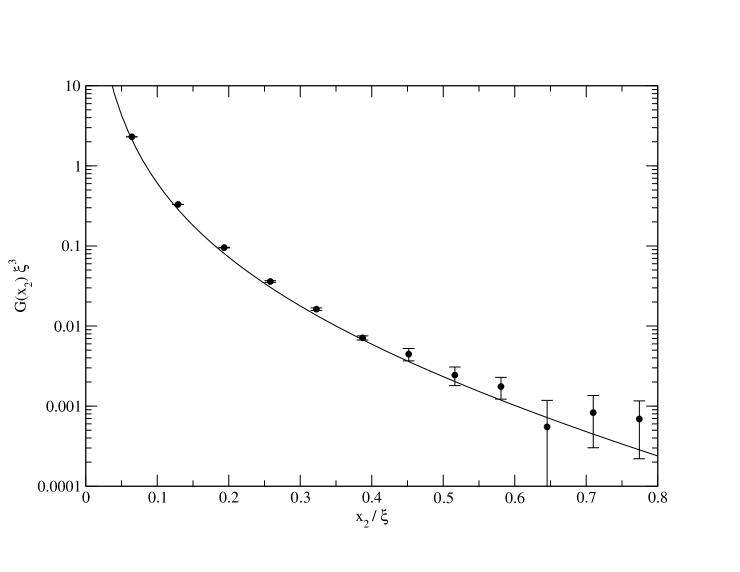
Figure 12: The point–to–time-slice correlator $G(x_{2})=\int_{0}^{L}dx_{1}\langle q(0)q(x)\rangle$ of the topological charge density (in units of $m^{3}=1/\xi^{3}$) as a function of $x_{2}/\xi$. The data points are extrapolations of Monte Carlo data obtained at $\xi/a=30.9(1)$ and $\xi/a=15.54(5)$ to the continuum limit, assuming ${\cal O}(a^{2})$ cut-off effects. At large distances, they are in good agreement with the analytic results of [69, 70] represented by the solid curve. We attribute the systematic deviations at short distances to not fully understood cut-off effects.

For the standard action a similar agreement had already been observed in [70]. In particular, this shows that some topological quantities make perfect sense in the continuum limit of the 2-d $O(3)$ model, despite the fact that $\chi_{t}$ is logarithmically divergent. The divergence is expected to also affect the energy density of $\theta$-vacua. Still, other physical quantities like the $\theta$-dependent mass gap should have a well-defined continuum limit, which is accessible using the meron-cluster algorithm.

5 Conclusions

We have investigated topological lattice actions for the 1-d $O(2)$ and $O(3)$ as well as for the 2-d $O(3)$ model. These actions are invariant against small deformations of the fields. Despite the fact that topological lattice actions do not have the correct classical continuum limit, as we have seen, they still yield the correct quantum continuum limit, irrespective of whether or not they explicitly suppress topological charges. In particular, it does not matter whether a topological action respects or violates a Schwarz inequality. Since, in contrast to other lattice actions, topological actions are invariant against small local deformations of the fields, one may have expected that they fall into a different universality class. However, the allowed local deformations are field-dependent and thus do not constitute a proper gauge symmetry of topological lattice models. In fact, even the standard action of a lattice $O(N)$ model has a field-dependent local $O(N-1)$ symmetry, since every spin can be rotated around the direction defined by the average of its nearest neighbors without changing the action value. Since such field-dependent local symmetries do not have the status of proper gauge symmetries, they have no impact on the corresponding universality class.

Since topological lattice actions do not suppress small fluctuations of the fields, perturbation theory is not applicable. We have seen that in one dimension topological lattice actions suffer from strong lattice artifacts of ${\cal O}(a)$. This seems to contradict Symanzik’s effective theory, which, however, does not apply in quantum mechanics. Despite the fact that lattice perturbation theory cannot be applied to topological lattice actions, Symanzik’s effective theory, which is formulated in the continuum, still describes the lattice artifacts of the 2-d $O(3)$ model with a topological lattice action. Interestingly, in contrast to the 1-d case, in the 2-d $O(3)$ model cut-off effects were observed to be less severe for a topological action than for the standard action, at least at practically accessible correlation lengths. Our results may encourage the use of unconventional regularizations, which might be advantageous from a computational point of view.

Although the topological angle-constraint action does not explicitly suppress dislocations, the corresponding topological susceptibility $\chi_{t}$ seems not to suffer from power-law divergences. Instead, the Monte Carlo data for $\chi_{t}$ are consistent with a logarithmic divergence, which already occurs in the continuum theory. The numerical results for the point–to–time-slice correlator $G(x_{2})=\int_{0}^{L}dx_{1}\langle q(0)q(x)\rangle$ of the topological charge density are consistent with the analytic predictions of [69, 70]. This underscores that, despite the fact that $\chi_{t}$ is logarithmically divergent, there exist topological physical quantities that have a well-defined continuum limit in the 2-d $O(3)$ model. Since the corresponding complex action problem can be solved using the meron-cluster algorithm, a numerical investigation of $\theta$-vacuum effects in the 2-d $O(3)$ model is both feasible and physically meaningful.

It is straightforward to construct topological lattice actions for Abelian and non-Abelian gauge theories. One may simply constrain the trace of a Wilson plaquette variable by some minimal value. Configurations that satisfy this constraint on all plaquettes can then be assigned a zero action value. It is conceivable that one can take algorithmic advantages from actions of this kind. It is an interesting subject for future studies to decide whether topological lattice actions may be useful in lattice Yang-Mills theory or in lattice QCD.

Our study underscores the robustness of universality, which, in particular, does not rely on classical concepts. Even when one uses actions that do not have the correct classical continuum limit, cannot be treated with perturbation theory, or do not obey a Schwarz inequality, the emerging quantum theory still has the correct continuum limit. This means that the standard approach of starting from a classical system and then quantizing it afterwards is not the only way to define a quantum theory. Even based on concepts that make no sense classically, one may still be able to construct a sensible quantum theory. Classical physics will then emerge dynamically from the underlying quantum system.

References

- [1] T. Reisz, Commun. Math. Phys. 116 (1988) 81.
- [2] T. Reisz, Nucl. Phys. B318 (1989) 417.
- [3] K. Symanzik, Nucl. Phys. B226 (1983) 187.
- [4] K. Symanzik, Nucl. Phys. B226 (1983) 205.
- [5] M. Lüscher and P. Weisz, Commun. Math. Phys. 97 (1985) 59.
- [6] M. Lüscher and P. Weisz, Phys. Lett. B158 (1985) 250.
- [7] P. Hasenfratz and F. Niedermayer, Nucl. Phys. B414 (1994) 785.
- [8] R. Burkhalter, Phys. Rev. D54 (1996) 4121.
- [9] R. Burkhalter, M. Imachi, Y. Shinno, and H. Yoneyama, Prog. Theor. Phys. 106 (2001) 613.
- [10] P. Hasenfratz, S. Hauswirth, T. Jörg, F. Niedermayer, and K. Holland, Nucl. Phys. B643 (2002) 280.
- [11] A. Patrascioiu and E. Seiler, J. Stat. Phys. 69 (1992) 573.
- [12] M. Aizenman, J. Stat. Phys. 77 (1994) 361.
- [13] A. Patrascioiu and E. Seiler, Nucl. Phys. Proc. Suppl. 30 (1993) 184.
- [14] A. Patrascioiu and E. Seiler, J. Stat. Phys. 106 (2002) 811.
- [15] M. Hasenbusch, Phys. Rev. D53 (1996) 3445.
- [16] M. Lüscher, Commun. Math. Phys. 85 (1982) 29.
- [17] W. Bietenholz, A. Pochinsky, and U.-J. Wiese, Phys. Rev. Lett. 75 (1995) 4524.
- [18] P. Hernández, K. Jansen, and M. Lüscher, Nucl. Phys. B552 (1999) 363.
- [19] M. Lüscher, Nucl. Phys. B549 (1999) 295.
- [20] M. Lüscher, Nucl. Phys. B568 (2000) 162.
- [21] H. Fukaya and T. Onogi, Phys. Rev. D68 (2003) 074503.
- [22] H. Fukaya and T. Onogi, Phys. Rev. D70 (2004) 054508.
- [23] H. Fukaya, S. Hashimoto, T. Hirohashi, K. Ogawa, and T. Onogi, Phys. Rev. D73 (2006) 014503.
- [24] W. Bietenholz, K. Jansen, K.-I. Nagai, S. Necco, L. Scorzato, and S. Shcheredin, JHEP 0603 (2006) 017.
- [25] E. Witten, Commun. Math. Phys. 117 (1988) 353.
- [26] A. D’Adda, M. Lüscher, and P. Di Vecchia, Nucl. Phys. B146 (1978) 63.
- [27] E. Vicari and H. Panagopoulos, Phys. Rep. 470 (2009) 93.
- [28] B. Berg and M. Lüscher, Nucl. Phys. B190 (1981) 412.
- [29] M. Lüscher, Nucl. Phys. B200 (1982) 61.
- [30] P. Schwab, Phys. Lett. B118 (1982) 373.
- [31] G. Münster, Phys. Lett. B118 (1982) 380.
- [32] M. Lüscher and D. Petcher, Nucl. Phys. B225 (1983) 53.
- [33] M. Blatter, R. Burkhalter, P. Hasenfratz, and F. Niedermayer, Phys. Rev. D53 (1996) 923.
- [34] E. Vicari, Nucl. Phys. B554 (1999) 301.
- [35] V. Azcoiti, A. Galante, and V. Laliena, Phys. Rev. Lett. 98 (2007) 257203.
- [36] M. Lüscher, Nucl. Phys. B205 (1982) 483.
- [37] D. J. R. Pugh and M. Teper, Phys. Lett. B324 (1989) 159.
- [38] M. Göckeler, A. S. Kronfeld, M. L. Laursen, G. Schierholz, and U.-J. Wiese, Phys. Lett. B233 (1989) 192.
- [39] A. Phillips and D. Stone, Commun. Math. Phys. 103 (1985) 599.
- [40] M. Göckeler, M. L. Laursen, G. Schierholz, and U.-J. Wiese, Commun. Math. Phys. 107 (1986) 467.
- [41] M. Göckeler, A. S. Kronfeld, M. L. Laursen, G. Schierholz, and U.-J. Wiese, Nucl. Phys. B292 (1987) 349.
- [42] W. Bietenholz, R. Brower, S. Chandrasekharan, and U.-J. Wiese, Phys. Lett. B407 (1997) 283.
- [43] P. H. Ginsparg and K. G. Wilson, Phys. Rev. D25 (1982) 2649.
- [44] P. Hasenfratz, V. Laliena, and F. Niedermayer, Phys. Lett. B427 (1998) 125.
- [45] L. Giusti, G. C. Rossi, and M. Testa, Phys. Lett. B587 (2004) 157.
- [46] M. Lüscher, Phys. Lett. B593 (2004) 296.
- [47] E. Witten, Nucl. Phys. B156 (1979) 269.
- [48] G. Veneziano, Nucl. Phys. B159 (1979) 213.
- [49] G. Veneziano, Phys. Lett. B95 (1980) 90.
- [50] L. Giusti, G. C. Rossi, M. Testa, and G. Veneziano, Nucl. Phys. B628 (2002) 234.
- [51] L. Del Debbio, L. Giusti and C. Pica, Phys. Rev. Lett. 94 (2005) 032003.
- [52] M. Lüscher and F. Palombi, arXiv:1008.0732 [hep-lat].
- [53] A. M. Polyakov and P. B. Wiegmann, Phys. Lett. B131 (1983) 121.
- [54] P. B. Wiegmann, Phys. Lett. B152 (1985) 209.
- [55] A. B. Zamolodchikov and A. B. Zamolodchikov, Ann. Phys. 120 (1979) 253.
- [56] P. Hasenfratz, M. Maggiore, and F. Niedermayer, Phys. Lett. B245 (1990) 522.
- [57] J. Balog und A. Hegedus, J. Phys. A: Math. Gen. 37 (2004) 1881.
- [58] M. Lüscher, P. Weisz, and U. Wolff, Nucl. Phys. B359 (1991) 221.
- [59] J. Balog, F. Niedermayer, and P. Weisz, Phys. Lett. B676 (2009) 188.
- [60] J. Balog, F. Niedermayer, and P. Weisz, Nucl. Phys. B824(2010) 563.
- [61] J. Balog, M. Niedermaier, F. Niedermayer, A. Patrascioiu, E. Seiler, and P. Weisz, Phys. Rev. D60 (1999) 094508.
- [62] U. Wolff, Phys. Rev. Lett. 62 (1989) 361.
- [63] U. Wolff, Nucl. Phys. B334 (1990) 581.
- [64] M. Campostrini, A. Pelissetto, P. Rossi, and E. Vicari, Phys. Lett. B402 (1997) 141.
- [65] S. Caracciolo, R. G. Edwards, A. Pelissetto, and A. D. Sokal, Phys. Rev. Lett. 75 (1995) 1891.
- [66] B. B. Beard, R. J. Birgeneau, M. Greven, and U.-J. Wiese, Phys. Rev. Lett. 80 (1998) 1742.
- [67] P. Hasenfratz and F. Niedermayer, Phys. Lett. B268 (1991) 231.
- [68] A. S. Kronfeld, M. L. Laursen, G. Schierholz, and U.-J. Wiese, Nucl. Phys. B292 (1987) 330.
- [69] J. Balog and M. Niedermaier, Nucl. Phys. B500 (1997) 421.
- [70] J. Balog and M. Niedermaier, Phys. Rev. Lett. 78 (1997) 4151.