Proximal Methods for Hierarchical Sparse Coding

Abstract

Sparse coding consists in representing signals as sparse linear combinations of atoms selected from a dictionary. We consider an extension of this framework where the atoms are further assumed to be embedded in a tree. This is achieved using a recently introduced tree-structured sparse regularization norm, which has proven useful in several applications. This norm leads to regularized problems that are difficult to optimize, and in this paper, we propose efficient algorithms for solving them. More precisely, we show that the proximal operator associated with this norm is computable exactly via a dual approach that can be viewed as the composition of elementary proximal operators. Our procedure has a complexity linear, or close to linear, in the number of atoms, and allows the use of accelerated gradient techniques to solve the tree-structured sparse approximation problem at the same computational cost as traditional ones using the $\ell_{1}$-norm. Our method is efficient and scales gracefully to millions of variables, which we illustrate in two types of applications: first, we consider fixed hierarchical dictionaries of wavelets to denoise natural images. Then, we apply our optimization tools in the context of dictionary learning, where learned dictionary elements naturally self-organize in a prespecified arborescent structure, leading to better performance in reconstruction of natural image patches. When applied to text documents, our method learns hierarchies of topics, thus providing a competitive alternative to probabilistic topic models.

Keywords: Proximal methods, dictionary learning, structured sparsity, matrix factorization.

1 Introduction

Modeling signals as sparse linear combinations of atoms selected from a dictionary has become a popular paradigm in many fields, including signal processing, statistics, and machine learning. This line of research, also known as sparse coding, has witnessed the development of several well-founded theoretical frameworks Tibshirani (1996); Chen et al. (1998); Mallat (1999); Tropp (2004, 2006); Wainwright (2009); Bickel et al. (2009) and the emergence of many efficient algorithmic tools Efron et al. (2004); Nesterov (2007); Beck and Teboulle (2009); Wright et al. (2009); Needell and Tropp (2009); Yuan et al. (2010).

In many applied settings, the structure of the problem at hand, such as, e.g., the spatial arrangement of the pixels in an image, or the presence of variables corresponding to several levels of a given factor, induces relationships between dictionary elements. It is appealing to use this a priori knowledge about the problem directly to constrain the possible sparsity patterns. For instance, when the dictionary elements are partitioned into predefined groups corresponding to different types of features, one can enforce a similar block structure in the sparsity pattern—that is, allow only that either all elements of a group are part of the signal decomposition or that all are dismissed simultaneously (see Yuan and Lin, 2006; Stojnic et al., 2009).

This example can be viewed as a particular instance of structured sparsity, which has been lately the focus of a large amount of research Baraniuk et al. (2010); Zhao et al. (2009); Huang et al. (2009); Jacob et al. (2009); Jenatton et al. (2009); Micchelli et al. (2010). In this paper, we concentrate on a specific form of structured sparsity, which we call hierarchical sparse coding: the dictionary elements are assumed to be embedded in a directed tree $\mathcal{T}$, and the sparsity patterns are constrained to form a connected and rooted subtree of $\mathcal{T}$ Donoho (1997); Baraniuk (1999); Baraniuk et al. (2002, 2010); Zhao et al. (2009); Huang et al. (2009). This setting extends more generally to a forest of directed trees.

In fact, such a hierarchical structure arises in many applications. Wavelet decompositions lend themselves well to this tree organization because of their multiscale structure, and benefit from it for image compression and denoising Shapiro (1993); Crouse et al. (1998); Baraniuk (1999); Baraniuk et al. (2002, 2010); He and Carin (2009); Zhao et al. (2009); Huang et al. (2009). In the same vein, edge filters of natural image patches can be represented in an arborescent fashion Zoran and Weiss (2009). Imposing these sparsity patterns has further proven useful in the context of hierarchical variable selection, e.g., when applied to kernel methods Bach (2008), to log-linear models for the selection of potential orders Schmidt and Murphy (2010), and to bioinformatics, to exploit the tree structure of gene networks for multi-task regression Kim and Xing (2010). Hierarchies of latent variables, typically used in neural networks and deep learning architectures (see Bengio, 2009, and references therein) have also emerged as a natural structure in several applications, notably to model text documents. In particular, in the context of topic models Blei et al. (2003), a hierarchical model of latent variables based on Bayesian non-parametric methods has been proposed by Blei et al. (2010) to model hierarchies of topics.

To perform hierarchical sparse coding, our work builds upon the approach of Zhao et al. (2009) who first introduced a sparsity-inducing norm $\Omega$ leading to this type of tree-structured sparsity pattern. We tackle the resulting nonsmooth convex optimization problem with proximal methods (e.g., Nesterov, 2007; Beck and Teboulle, 2009; Wright et al., 2009; Combettes and Pesquet, 2010) and we show in this paper that its key step, the computation of the proximal operator, can be solved exactly with a complexity linear, or close to linear, in the number of dictionary elements—that is, with the same complexity as for classical $\ell_{1}$-sparse decomposition problems Tibshirani (1996); Chen et al. (1998). Concretely, given an $m$-dimensional signal ${\mathbf{x}}$ along with a dictionary ${\mathbf{D}}=[{\mathbf{d}}^{1},\dots,{\mathbf{d}}^{p}]\in\mathbb{R}^{m\times p}$ composed of $p$ atoms, the optimization problem at the core of our paper can be written as

$$\min_{{\boldsymbol{\alpha}}\in\mathbb{R}^{p}}\dfrac{1}{2}\|{\mathbf{x}}-{\mathbf{D}}{\boldsymbol{\alpha}}\|^{2}_{2}+\lambda\Omega({\boldsymbol{\alpha}}),\ \mathrm{with}\ \lambda\geq 0.$$

In this formulation, the sparsity-inducing norm $\Omega$ encodes a hierarchical structure among the atoms of ${\mathbf{D}}$, where this structure is assumed to be known beforehand. The precise meaning of hierarchical structure and the definition of $\Omega$ will be made more formal in the next sections. A particular instance of this problem—known as the proximal problem—is central to our analysis and concentrates on the case where the dictionary ${\mathbf{D}}$ is orthogonal.

In addition to a speed benchmark that evaluates the performance of our proposed approach in comparison with other convex optimization techniques, two types of applications and experiments are considered. First, we consider settings where the dictionary is fixed and given a priori, corresponding for instance to a basis of wavelets for the denoising of natural images. Second, we show how one can take advantage of this hierarchical sparse coding in the context of dictionary learning Olshausen and Field (1997); Aharon et al. (2006); Mairal et al. (2010a), where the dictionary is learned to adapt to the predefined tree structure. This extension of dictionary learning is notably shown to share interesting connections with hierarchical probabilistic topic models.

To summarize, the contributions of this paper are threefold:

• We show that the proximal operator for a tree-structured sparse regularization can be computed exactly in a finite number of operations using a dual approach. Our approach is equivalent to computing a particular sequence of elementary proximal operators, and has a complexity linear, or close to linear, in the number of variables. Accelerated gradient methods (e.g., Nesterov, 2007; Beck and Teboulle, 2009; Combettes and Pesquet, 2010) can then be applied to solve large-scale tree-structured sparse decomposition problems at the same computational cost as traditional ones using the $\ell_{1}$-norm.

• We propose to use this regularization scheme to learn dictionaries embedded in a tree, which, to the best of our knowledge, has not been done before in the context of structured sparsity.

• Our method establishes a bridge between hierarchical dictionary learning and hierarchical topic models Blei et al. (2010), which builds upon the interpretation of topic models as multinomial PCA Buntine (2002), and can learn similar hierarchies of topics. This point is discussed in Sections 5.5 and 6.

Note that this paper extends a shorter version published in the proceedings of the international conference of machine learning Jenatton et al. (2010).

1.1 Notation

Vectors are denoted by bold lower case letters and matrices by upper case ones. We define for $q\geq 1$ the $\ell_{q}$-norm of a vector ${\mathbf{x}}$ in ${\mathbb{R}}^{m}$ as $\|{\mathbf{x}}\|_{q}\stackrel{{\scriptstyle\vartriangle}}{{=}}(\sum_{i=1}^{m}|{\mathbf{x}}_{i}|^{q})^{{1}/{q}}$, where ${\mathbf{x}}_{i}$ denotes the $i$-th coordinate of ${\mathbf{x}}$, and $\|{\mathbf{x}}\|_{\infty}\stackrel{{\scriptstyle\vartriangle}}{{=}}\max_{i=1,\ldots,m}|{\mathbf{x}}_{i}|=\lim_{q\to\infty}\|{\mathbf{x}}\|_{q}$. We also define the $\ell_{0}$-pseudo-norm as the number of nonzero elements in a vector: $\|{\mathbf{x}}\|_{0}\stackrel{{\scriptstyle\vartriangle}}{{=}}\#\{i~{}~{}\text{s.t.}~{}~{}{\mathbf{x}}_{i}\neq 0\}=\lim_{q\to 0^{+}}(\sum_{i=1}^{m}|{\mathbf{x}}_{i}|^{q})$. We consider the Frobenius norm of a matrix ${\mathbf{X}}$ in ${\mathbb{R}}^{m\times n}$: $\|{\mathbf{X}}\|_{\text{F}}\stackrel{{\scriptstyle\vartriangle}}{{=}}(\sum_{i=1}^{m}\sum_{j=1}^{n}{\mathbf{X}}_{ij}^{2})^{{1}/{2}}$, where ${\mathbf{X}}_{ij}$ denotes the entry of ${\mathbf{X}}$ at row $i$ and column $j$. Finally, for a scalar $y$, we denote $(y)_{+}\stackrel{{\scriptstyle\vartriangle}}{{=}}\max(y,0)$.

The rest of this paper is organized as follows: Section 2 presents related work and the problem we consider. Section 3 is devoted to the algorithm we propose, and Section 4 introduces the dictionary learning framework and shows how it can be used with tree-structured norms. Section 5 presents several experiments demonstrating the effectiveness of our approach and Section 6 concludes the paper.

2 Problem Statement and Related Work

Let us consider an input signal of dimension $m$, typically an image described by its $m$ pixels, which we represent by a vector ${\mathbf{x}}$ in $\mathbb{R}^{m}$. In traditional sparse coding, we seek to approximate this signal by a sparse linear combination of atoms, or dictionary elements, represented here by the columns of a matrix ${\mathbf{D}}\stackrel{{\scriptstyle\vartriangle}}{{=}}[{\mathbf{d}}^{1},\dots,{\mathbf{d}}^{p}]$ in $\mathbb{R}^{m\times p}$. This can equivalently be expressed as ${\mathbf{x}}\approx{\mathbf{D}}{\boldsymbol{\alpha}}$ for some sparse vector ${\boldsymbol{\alpha}}$ in $\mathbb{R}^{p}$, i.e, such that the number of nonzero coefficients $\|{\boldsymbol{\alpha}}\|_{0}$ is small compared to $p$. The vector ${\boldsymbol{\alpha}}$ is referred to as the code, or decomposition, of the signal ${\mathbf{x}}$.

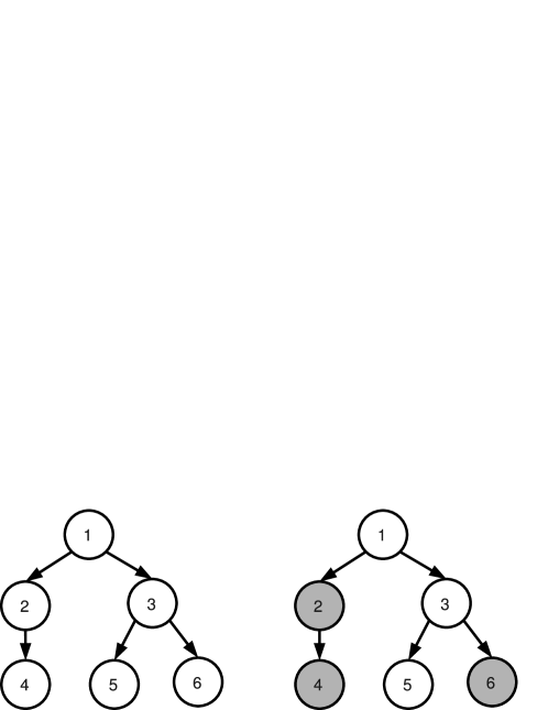
Figure 1: Example of a tree ${\mathcal{T}}$ when $p=6$. With the rule we consider for the nonzero patterns, if we have ${\boldsymbol{\alpha}}_{5}\neq 0$, we must also have ${\boldsymbol{\alpha}}_{k}\neq 0$ for $k$ in $\text{ancestors}(5)=\{1,3,5\}$.

In the rest of the paper, we focus on specific sets of nonzero coefficients—or simply, nonzero patterns—for the decomposition vector ${\boldsymbol{\alpha}}$. In particular, we assume that we are given a tree ${\mathcal{T}}$ whose $p$ nodes are indexed by $j$ in $\{1,\dots,p\}$. We want the nonzero patterns of ${\boldsymbol{\alpha}}$ to form a connected and rooted subtree of ${\mathcal{T}}$; in other words, if $\text{ancestors}(j)\subseteq\{1,\dots,p\}$ denotes the set of indices corresponding to the ancestors of the node $j$ in ${\mathcal{T}}$ (see Figure 1), the vector ${\boldsymbol{\alpha}}$ obeys the following rule

$${\boldsymbol{\alpha}}_{j}\neq 0\Rightarrow[\,{\boldsymbol{\alpha}}_{k}\neq 0\ \text{for all}\ k\ \text{in ancestors}(j)\,].$$ (1)

Informally, we want to exploit the structure of ${\mathcal{T}}$ in the following sense: the decomposition of any signal ${\mathbf{x}}$ can involve a dictionary element ${\mathbf{d}}^{j}$ only if the ancestors of ${\mathbf{d}}^{j}$ in the tree ${\mathcal{T}}$ are themselves part of the decomposition.

We now review previous work that has considered the sparse approximation problem with tree-structured constraints (1). Similarly to traditional sparse coding, there are basically two lines of research, that either (A) deal with nonconvex and combinatorial formulations that are in general computationally intractable and addressed with greedy algorithms, or (B) concentrate on convex relaxations solved with convex programming methods.

2.1 Nonconvex Approaches

For a given sparsity level $s\geq 0$ (number of nonzero coefficients), the following nonconvex problem

$$\min_{\begin{subarray}{c}{\boldsymbol{\alpha}}\in\mathbb{R}^{p}\\ \|{\boldsymbol{\alpha}}\|_{0}\leq s\end{subarray}}\frac{1}{2}\|{\mathbf{x}}-{\mathbf{D}}{\boldsymbol{\alpha}}\|_{2}^{2}\quad\text{such that}\ \text{condition~{}(\ref{eq:ancestor_cond}) is respected},$$ (2)

has been tackled by Baraniuk (1999); Baraniuk et al. (2002) in the context of wavelet approximations with a greedy procedure. A penalized version of problem (2) (that adds $\lambda\|{\boldsymbol{\alpha}}\|_{0}$ to the objective function in place of the constraint $\|{\boldsymbol{\alpha}}\|_{0}\leq s$) has been considered by Donoho (1997), while studying the more general problem of best approximation from dyadic partitions (see Section 6 in Donoho, 1997). Interestingly, the algorithm we introduce in Section 3 shares conceptual links with the dynamic-programming approach of Donoho (1997), which was also used by Baraniuk et al. (2010), in the sense that the same order of traversal of the tree is used in both procedures. We investigate more thoroughly the relations between our algorithm and this approach in Appendix A.

Problem (2) has been further studied for structured compressive sensing Baraniuk et al. (2010), with a greedy algorithm that builds upon Needell and Tropp (2009). Finally, Huang et al. (2009) have proposed a formulation related to (2), with a nonconvex penalty based on an information-theoretic criterion.

2.2 Convex Approach

We now turn to a convex reformulation of the constraint (1), which is the starting point for the convex optimization tools we develop in Section 3.

2.2.1 Hierarchical Sparsity-Inducing Norms

Condition (1) can be equivalently expressed by its contrapositive, thus leading to an intuitive way of penalizing the vector ${\boldsymbol{\alpha}}$ to obtain tree-structured nonzero patterns. More precisely, defining $\text{descendants}(j)\subseteq\{1,\dots,p\}$ analogously to $\text{ancestors}(j)$ for $j$ in $\{1,\dots,p\}$, condition (1) amounts to saying that if a dictionary element is not used in the decomposition, its descendants in the tree should not be used either. Formally, this can be formulated as:

$${\boldsymbol{\alpha}}_{j}=0\Rightarrow[\,{\boldsymbol{\alpha}}_{k}=0\ \text{for all}\ k\ \text{in descendants}(j)\,].$$ (3)

From now on, we denote by $\mathcal{G}$ the set defined by $\mathcal{G}\stackrel{{\scriptstyle\vartriangle}}{{=}}\{\text{descendants}(j);j\in\{1,\dots,p\}\},$ and refer to each member $g$ of $\mathcal{G}$ as a group (Figure 2). To obtain a decomposition with the desired property (3), one can naturally penalize the number of groups $g$ in $\mathcal{G}$ that are “involved” in the decomposition of ${\mathbf{x}}$, i.e., that record at least one nonzero coefficient of ${\boldsymbol{\alpha}}$:

$$\sum_{g\in\mathcal{G}}\delta^{g},\ \text{with}\ \delta^{g}\stackrel{{\scriptstyle\vartriangle}}{{=}}\begin{cases}1&\text{if there exists}\ j\in g\ \text{such that}\ {\boldsymbol{\alpha}}_{j}\neq 0,\\ 0&\text{otherwise}.\end{cases}$$ (4)

While this intuitive penalization is nonconvex (and not even continuous), a convex proxy has been introduced by Zhao et al. (2009). It was further considered by Bach (2008); Kim and Xing (2010); Schmidt and Murphy (2010) in several different contexts. For any vector ${\boldsymbol{\alpha}}\in\mathbb{R}^{p}$, let us define

$$\Omega({\boldsymbol{\alpha}})\stackrel{{\scriptstyle\vartriangle}}{{=}}\sum_{g\in\mathcal{G}}\omega_{g}\|{\boldsymbol{\alpha}}_{{{\scriptscriptstyle\mid}g}}\|,$$

where ${\boldsymbol{\alpha}}_{{{\scriptscriptstyle\mid}g}}$ is the vector of size $p$ whose coordinates are equal to those of ${\boldsymbol{\alpha}}$ for indices in the set $g$, and to $0$ otherwise. The notation $\|.\|$ stands in practice either for the $\ell_{2}$- or $\ell_{\infty}$-norm, and $(\omega_{g})_{g\in\mathcal{G}}$ denotes some positive weights. As analyzed by Zhao et al. (2009) and Jenatton et al. (2009), when penalizing by $\Omega$, some of the vectors ${\boldsymbol{\alpha}}_{{{\scriptscriptstyle\mid}g}}$ are set to zero for some $g\in\mathcal{G}$. Therefore, the components of ${\boldsymbol{\alpha}}$ corresponding to some complete subtrees of $\mathcal{T}$ are set to zero, which exactly matches condition (3), as illustrated in Figure 2.

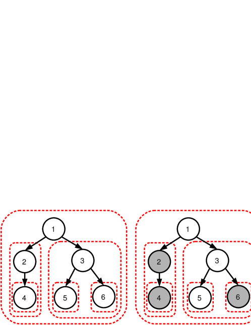
Figure 2: Left: example of a tree-structured set of groups $\mathcal{G}$ (dashed contours in red), corresponding to a tree $\mathcal{T}$ with $p=6$ nodes represented by black circles. Right: example of a sparsity pattern induced by the tree-structured norm corresponding to $\mathcal{G}$: the groups $\{2,4\},\{4\}$ and $\{6\}$ are set to zero, so that the corresponding nodes (in gray) that form subtrees of $\mathcal{T}$ are removed. The remaining nonzero variables $\{1,3,5\}$ form a rooted and connected subtree of $\mathcal{T}$. This sparsity pattern obeys the following equivalent rules: (i) if a node is selected, the same goes for all its ancestors. (ii) if a node is not selected, then its descendant are not selected.

Note that although we presented for simplicity this hierarchical norm in the context of a single tree with a single element at each node, it can easily be extended to the case of forests of trees, and/or trees containing arbitrary numbers of dictionary elements at each node (with nodes possibly containing no dictionary element). More broadly, this formulation can be extended with the notion of tree-structured groups, which we now present:

Definition 1 (Tree-structured set of groups.)

A set of groups $\mathcal{G}\!\stackrel{{\scriptstyle\vartriangle}}{{=}}\!\{g\}_{g\in\mathcal{G}}$ is said to be tree-structured in $\{1,\dots,p\}$, if $\,\bigcup_{g\in\mathcal{G}}\!g=\{1,\dots,p\}$ and if for all $g,h\in\mathcal{G}$, $(g\cap h\neq\emptyset)\Rightarrow(g\subseteq h\ \text{or}\ h\subseteq g).$ For such a set of groups, there exists a (non-unique) total order relation $\preceq$ such that:

$$g\preceq h\;\Rightarrow\;\big{\{}g\subseteq h\text{~{}~{}~{}or~{}~{}~{}}g\cap h=\emptyset\big{\}}.$$

Given such a tree-structured set of groups $\mathcal{G}$ and its associated norm $\Omega$, we are interested throughout the paper in the following hierarchical sparse coding problem,

$$\min_{{\boldsymbol{\alpha}}\in\mathbb{R}^{p}}f({\boldsymbol{\alpha}})+\lambda\Omega({\boldsymbol{\alpha}}),$$ (5)

where $\Omega$ is the tree-structured norm we have previously introduced, the non-negative scalar $\lambda$ is a regularization parameter controlling the sparsity of the solutions of (5), and $f$ a smooth convex loss function (see Section 3 for more details about the smoothness assumptions on $f$). In the rest of the paper, we will mostly use the square loss $f({\boldsymbol{\alpha}})=\frac{1}{2}\|{\mathbf{x}}-{\mathbf{D}}{\boldsymbol{\alpha}}\|^{2}_{2},$ with a dictionary ${\mathbf{D}}$ in ${\mathbb{R}}^{m\times p}$, but the formulation of Eq. (5) extends beyond this context. In particular one can choose $f$ to be the logistic loss, which is commonly used for classification problems (e.g., see Hastie et al., 2009).

Before turning to optimization methods for the hierarchical sparse coding problem, we consider a particular instance. The sparse group Lasso was recently considered by Sprechmann et al. (2010) and Friedman et al. (2010) as an extension of the group Lasso of Yuan and Lin (2006). To induce sparsity both groupwise and within groups, Sprechmann et al. (2010) and Friedman et al. (2010) add an $\ell_{1}$ term to the regularization of the group Lasso, which given a partition $\mathcal{P}$ of $\{1,\ldots,p\}$ in disjoint groups yields a regularized problem of the form

$$\min_{{\boldsymbol{\alpha}}\in{\mathbb{R}}^{p}}\dfrac{1}{2}\|{\mathbf{x}}-{\mathbf{D}}{\boldsymbol{\alpha}}\|^{2}_{2}+\lambda\sum_{g\in\mathcal{P}}\|{\boldsymbol{\alpha}}_{{{\scriptscriptstyle\mid}g}}\|_{2}+\lambda^{\prime}\|{\boldsymbol{\alpha}}\|_{1}.$$

Since $\mathcal{P}$ is a partition, the set of groups in $\mathcal{P}$ and the singletons form together a tree-structured set of groups according to definition 1 and the algorithm we will develop is therefore applicable to this problem.

2.2.2 Optimization for Hierarchical Sparsity-Inducing Norms

While generic approaches like interior-point methods Boyd and Vandenberghe (2004) and subgradient descent schemes Bertsekas (1999) might be used to deal with the nonsmooth norm $\Omega$, several dedicated procedures have been proposed.

In Zhao et al. (2009), a boosting-like technique is used, with a path-following strategy in the specific case where $\|.\|$ is the $\ell_{\infty}$-norm. Based on the variational equality

$$\|{\mathbf{u}}\|_{1}=\min_{{\mathbf{z}}\in\mathbb{R}^{p}_{+}}\dfrac{1}{2}\big{[}\sum_{j=1}^{p}\dfrac{{\mathbf{u}}_{j}^{2}}{{\mathbf{z}}_{j}}+{\mathbf{z}}_{j}\big{]},$$ (6)

Kim and Xing (2010) follow a reweighted least-square scheme that is well adapted to the square loss function. To the best of our knowledge, a formulation of this type is however not available when $\|.\|$ is the $\ell_{\infty}$-norm. In addition it requires an appropriate smoothing to become provably convergent. The same approach is considered by Bach (2008), but built upon an active-set strategy. Other proposed methods consist of a projected gradient descent with approximate projections onto the ball $\{{\mathbf{u}}\in\mathbb{R}^{p};\,\Omega({\mathbf{u}})\leq\lambda\}$ Schmidt and Murphy (2010), and an augmented-Lagrangian based technique Sprechmann et al. (2010) for solving a particular case with two-level hierarchies.

While the previously listed first-order approaches are (1) loss-function dependent, and/or (2) not guaranteed to achieve optimal convergence rates, and/or (3) not able to yield sparse solutions without a somewhat arbitrary post-processing step, we propose to resort to proximal methods that do not suffer from any of these drawbacks.

3 Optimization

We begin with a brief introduction to proximal methods, necessary to present our contributions. From now on, we assume that $f$ is convex and continuously differentiable with Lipschitz-continuous gradient. It is worth mentioning that there exist various proximal schemes in the literature that differ in their settings (e.g., batch versus stochastic) and/or the assumptions made on $f$. For instance, the material we develop in this paper could also be applied to online/stochastic frameworks (Duchi and Singer, 2009; Hu et al., 2009; Xiao, 2010) and to possibly nonsmooth functions $f$ (e.g., Duchi and Singer, 2009; Xiao, 2010; Combettes and Pesquet, 2010, and references therein). Finally, most of the technical proofs of this section are presented in Appendix B for readability.

3.1 Proximal Operator for the Norm $\Omega$

Proximal methods have drawn increasing attention in the signal processing (e.g., Becker et al., 2009; Wright et al., 2009; Combettes and Pesquet, 2010, and numerous references therein) and the machine learning communities (e.g., Bach et al., 2011, and references therein), especially because of their convergence rates (optimal for the class of first-order techniques) and their ability to deal with large nonsmooth convex problems (e.g., Nesterov, 2007; Beck and Teboulle, 2009). In a nutshell, these methods can be seen as a natural extension of gradient-based techniques when the objective function to minimize has a nonsmooth part. Proximal methods are iterative procedures. The simplest version of this class of methods linearizes at each iteration the function $f$ around the current estimate $\hat{{\boldsymbol{\alpha}}}$, and this estimate is updated as the (unique by strong convexity) solution of the proximal problem, defined as follows:

$$\min_{{\boldsymbol{\alpha}}\in\mathbb{R}^{p}}~{}f(\hat{{\boldsymbol{\alpha}}})+({\boldsymbol{\alpha}}-\hat{{\boldsymbol{\alpha}}})^{\top}\nabla\!f(\hat{{\boldsymbol{\alpha}}})+\lambda\Omega({\boldsymbol{\alpha}})+\frac{L}{2}\|{\boldsymbol{\alpha}}-\hat{{\boldsymbol{\alpha}}}\|_{2}^{2}.$$

The quadratic term keeps the update in a neighborhood where $f$ is close to its linear approximation, and $L\!>\!0$ is a parameter which is an upper bound on the Lipschitz constant of $\nabla f$. This problem can be equivalently rewritten as:

$$\min_{{\boldsymbol{\alpha}}\in\mathbb{R}^{p}}~{}\frac{1}{2}\Big{\|}{\boldsymbol{\alpha}}-\big{(}\hat{{\boldsymbol{\alpha}}}-\frac{1}{L}\nabla\!f(\hat{{\boldsymbol{\alpha}}})\big{)}\Big{\|}_{2}^{2}+\frac{\lambda}{L}\Omega({\boldsymbol{\alpha}}).$$

Solving efficiently and exactly this problem is crucial to enjoy the fast convergence rates of proximal methods. In addition, when the nonsmooth term $\Omega$ is not present, the previous proximal problem exactly leads to the standard gradient update rule. More generally, we define the proximal operator:

Definition 2 (Proximal Operator)

The proximal operator associated with our regularization term $\lambda\Omega$, which we denote by $\text{Prox}_{\lambda\Omega}$, is the function that maps a vector ${\mathbf{u}}\in\mathbb{R}^{p}$ to the unique solution of

$$\min_{{\mathbf{v}}\in\mathbb{R}^{p}}\frac{1}{2}\|{\mathbf{u}}-{\mathbf{v}}\|_{2}^{2}+\lambda\Omega({\mathbf{v}}).$$ (7)

This operator was initially introduced by Moreau (1962) to generalize the projection operator onto a convex set. What makes proximal methods appealing for solving sparse decomposition problems is that this operator can be often computed in closed-form. For instance,

• When $\Omega$ is the $\ell_{1}$-norm—that is, $\Omega({\mathbf{u}})=\|{\mathbf{u}}\|_{1}$, the proximal operator is the well-known elementwise soft-thresholding operator,

  $$\forall j\in\{1,\ldots,p\},~{}~{}{\mathbf{u}}_{j}\mapsto\operatorname{sign}({\mathbf{u}}_{j})(|{\mathbf{u}}_{j}|-\lambda)_{+}~{}~{}~{}=\begin{cases}0&\text{if}~{}~{}|{\mathbf{u}}_{j}|\leq\lambda\\ \operatorname{sign}({\mathbf{u}}_{j})(|{\mathbf{u}}_{j}|-\lambda)&\text{otherwise}.\end{cases}$$

• When $\Omega$ is a group-Lasso penalty with $\ell_{2}$-norms—that is, $\Omega({\mathbf{u}})=\sum_{g\in\mathcal{G}}\|{\mathbf{u}}_{{{\scriptscriptstyle\mid}g}}\|_{2}$, with $\mathcal{G}$ being a partition of $\{1,\ldots,p\}$, the proximal problem is separable in every group, and the solution is a generalization of the soft-thresholding operator to groups of variables:

  $$\forall g\in\mathcal{G}~{}~{},{\mathbf{u}}_{{{\scriptscriptstyle\mid}g}}\mapsto{\mathbf{u}}_{{{\scriptscriptstyle\mid}g}}-\Pi_{\|.\|_{2}\leq\lambda}[{\mathbf{u}}_{{{\scriptscriptstyle\mid}g}}]=\begin{cases}0&\text{if}~{}~{}\|{\mathbf{u}}_{{{\scriptscriptstyle\mid}g}}\|_{2}\leq\lambda\\ \frac{\|{\mathbf{u}}_{{{\scriptscriptstyle\mid}g}}\|_{2}-\lambda}{\|{\mathbf{u}}_{{{\scriptscriptstyle\mid}g}}\|_{2}}{\mathbf{u}}_{{{\scriptscriptstyle\mid}g}}&\text{otherwise},\\ \end{cases}$$

  where $\Pi_{\|.\|_{2}\leq\lambda}$ denotes the orthogonal projection onto the ball of the $\ell_{2}$-norm of radius $\lambda$.

• When $\Omega$ is a group-Lasso penalty with $\ell_{\infty}$-norms—that is, $\Omega({\mathbf{u}})=\sum_{g\in\mathcal{G}}\|{\mathbf{u}}_{{{\scriptscriptstyle\mid}g}}\|_{\infty}$, the solution is also a group-thresholding operator:

  $$\forall g\in\mathcal{G},~{}~{}{\mathbf{u}}_{{{\scriptscriptstyle\mid}g}}\mapsto{\mathbf{u}}_{{{\scriptscriptstyle\mid}g}}-\Pi_{\|.\|_{1}\leq\lambda}[{\mathbf{u}}_{{{\scriptscriptstyle\mid}g}}],$$

  where $\Pi_{\|.\|_{1}\leq\lambda}$ denotes the orthogonal projection onto the $\ell_{1}$-ball of radius $\lambda$, which can be solved in $O(p)$ operations Brucker (1984); Maculan and Galdino de Paula (1989). Note that when $\|{\mathbf{u}}_{{{\scriptscriptstyle\mid}g}}\|_{1}\leq\lambda$, we have a group-thresholding effect, with ${\mathbf{u}}_{{{\scriptscriptstyle\mid}g}}-\Pi_{\|.\|_{1}\leq\lambda}[{\mathbf{u}}_{{{\scriptscriptstyle\mid}g}}]=0$.

More generally, a classical result (see, e.g., Combettes and Pesquet, 2010; Wright et al., 2009) says that the proximal operator for a norm $\|.\|$ can be computed as the residual of the projection of a vector onto a ball of the dual-norm denoted by $\|.\|_{\ast}$, and defined for any vector ${\boldsymbol{\kappa}}$ in ${\mathbb{R}}^{p}$ by $\|{\boldsymbol{\kappa}}\|_{\ast}\stackrel{{\scriptstyle\vartriangle}}{{=}}\max_{\|{\mathbf{z}}\|\leq 1}{\mathbf{z}}^{\top}{\boldsymbol{\kappa}}$. This is a classical duality result for proximal operators leading to the different closed forms we have just presented. We have indeed that $\text{Prox}_{\lambda\|.\|_{2}}=\text{Id}-\Pi_{\|.\|_{2}\leq\lambda}$ and $\text{Prox}_{\lambda\|.\|_{\infty}}=\text{Id}-\Pi_{\|.\|_{1}\leq\lambda}$, where Id stands for the identity operator. Obtaining closed forms is, however, not possible anymore as soon as some groups in $\mathcal{G}$ overlap, which is always the case in our hierarchical setting with tree-structured groups.

3.2 A Dual Formulation of the Proximal Problem

We now show that Eq. (7) can be solved using a dual approach, as described in the following lemma. The result relies on conic duality Boyd and Vandenberghe (2004), and does not make any assumption on the choice of the norm $\|.\|$:

Lemma 1 (Dual of the proximal problem)

Let ${\mathbf{u}}\in\mathbb{R}^{p}$ and let us consider the problem

$$\begin{split}&\max_{{\boldsymbol{\xi}}\in\mathbb{R}^{p\times|\mathcal{G}|}}-\frac{1}{2}\Big{[}\Big{\|}{\mathbf{u}}-\sum_{g\in\mathcal{G}}{\boldsymbol{\xi}}^{g}\Big{\|}^{2}_{2}-\|{\mathbf{u}}\|_{2}^{2}\Big{]}\\ \mbox{ s.t. }&\forall g\in\mathcal{G},\ \|{\boldsymbol{\xi}}^{g}\|_{\ast}\leq\lambda\omega_{g}\mbox{ and }\,{\boldsymbol{\xi}}^{g}_{j}=0\,\mbox{ if }\,j\notin g,\end{split}$$ (8)

where ${\boldsymbol{\xi}}=({\boldsymbol{\xi}}^{g})_{g\in\mathcal{G}}$ and ${\boldsymbol{\xi}}^{g}_{j}$ denotes the $j$-th coordinate of the vector ${\boldsymbol{\xi}}^{g}$ in $\mathbb{R}^{p}$. Then, problems (7) and (8) are dual to each other and strong duality holds. In addition, the pair of primal-dual variables $\{{\mathbf{v}},{\boldsymbol{\xi}}\}$ is optimal if and only if ${\boldsymbol{\xi}}$ is a feasible point of the optimization problem (8), and

$${\textstyle{\mathbf{v}}={\mathbf{u}}-\sum_{g\in\mathcal{G}}{\boldsymbol{\xi}}^{g}}\quad\mathrm{and}\quad\forall g\in\mathcal{G},\ {\boldsymbol{\xi}}^{g}=\Pi_{\|.\|_{\ast}\leq\lambda\omega_{g}}({\mathbf{v}}_{{{\scriptscriptstyle\mid}g}}+{\boldsymbol{\xi}}^{g}),$$ (9)

where we denote by $\Pi_{\|.\|_{\ast}\leq\lambda\omega_{g}}$ the orthogonal projection onto the ball $\{{\boldsymbol{\kappa}}\in\mathbb{R}^{p};\ \|{\boldsymbol{\kappa}}\|_{\ast}\leq\lambda\omega_{g}\}$.

Note that we focus here on specific tree-structured groups, but the previous lemma is valid regardless of the nature of $\mathcal{G}$. The rationale of introducing such a dual formulation is to consider an equivalent problem to (7) that removes the issue of overlapping groups at the cost of a larger number of variables. In Eq. (7), one is indeed looking for a vector ${\mathbf{v}}$ of size $p$, whereas one is considering a matrix ${\boldsymbol{\xi}}$ in ${\mathbb{R}}^{p\times|\mathcal{G}|}$ in Eq. (8) with $\sum_{g\in\mathcal{G}}|g|$ nonzero entries, but with separable (convex) constraints for each of its columns.

This specific structure makes it possible to use block coordinate ascent Bertsekas (1999). Such a procedure is presented in Algorithm 1. It optimizes sequentially Eq. (8) with respect to the variable ${\boldsymbol{\xi}}^{g}$, while keeping fixed the other variables ${\boldsymbol{\xi}}^{h}$, for $h\neq g$. It is easy to see from Eq. (8) that such an update of a column ${\boldsymbol{\xi}}^{g}$, for a group $g$ in $\mathcal{G}$, amounts to computing the orthogonal projection of the vector ${\mathbf{u}}_{{{\scriptscriptstyle\mid}g}}-\sum_{h\neq g}\xi_{{{\scriptscriptstyle\mid}g}}^{h}$ onto the ball of radius $\lambda\omega_{g}$ of the dual norm $\|.\|_{\ast}$.

Algorithm 1 Block coordinate ascent in the dual

  Inputs: ${\mathbf{u}}\in\mathbb{R}^{p}$ and set of groups $\mathcal{G}$.

  Outputs: $({\mathbf{v}},{\boldsymbol{\xi}})$ (primal-dual solutions).

  Initialization: ${\boldsymbol{\xi}}={\mathbf{0}}$.

  while  ( maximum number of iterations not reached )  do

     for  $g\in\mathcal{G}$  do

        ${\boldsymbol{\xi}}^{g}\leftarrow\Pi_{\|.\|_{\ast}\leq\lambda\omega_{g}}(\big{[}{\mathbf{u}}-\sum_{h\neq g}{\boldsymbol{\xi}}^{h}\big{]}_{{{\scriptscriptstyle\mid}g}})$.

     end for

  end while

  ${\mathbf{v}}\leftarrow{\mathbf{u}}-\sum_{g\in\mathcal{G}}{\boldsymbol{\xi}}^{g}$.

3.3 Convergence in One Pass

In general, Algorithm 1 is not guaranteed to solve exactly Eq. (7) in a finite number of iterations. However, when $\|.\|$ is the $\ell_{2}$- or $\ell_{\infty}$-norm, and provided that the groups in $\mathcal{G}$ are appropriately ordered, we now prove that only one pass of Algorithm 1, i.e., only one iteration over all groups, is sufficient to obtain the exact solution of Eq. (7). This result constitutes the main technical contribution of the paper and is the key for the efficiency of our procedure.

Before stating this result, we need to introduce a lemma showing that, given two nested groups $g,h$ such that $g\subseteq h\subseteq\{1,\dots,p\}$, if ${\boldsymbol{\xi}}^{g}$ is updated before ${\boldsymbol{\xi}}^{h}$ in Algorithm 1, then the optimality condition for ${\boldsymbol{\xi}}^{g}$ is not perturbed by the update of ${\boldsymbol{\xi}}^{h}$.

Lemma 2 (Projections with nested groups)

Let $\|.\|$ denote either the $\ell_{2}$- or $\ell_{\infty}$-norm, and $g$ and $h$ be two nested groups—that is, $g\subseteq h\subseteq\{1,\dots,p\}$. Let ${\mathbf{u}}$ be a vector in $\mathbb{R}^{p}$, and let us consider the successive projections

$${\boldsymbol{\xi}}^{g}\stackrel{{\scriptstyle\vartriangle}}{{=}}\Pi_{\|.\|_{\ast}\leq t_{g}}({\mathbf{u}}_{{{\scriptscriptstyle\mid}g}})~{}\text{ and }~{}{\boldsymbol{\xi}}^{h}\stackrel{{\scriptstyle\vartriangle}}{{=}}\Pi_{\|.\|_{\ast}\leq t_{h}}({\mathbf{u}}_{{{\scriptscriptstyle\mid}h}}-{\boldsymbol{\xi}}^{g}),$$

with $t_{g},t_{h}>0$. Let us introduce ${\mathbf{v}}={\mathbf{u}}-{\boldsymbol{\xi}}^{g}-{\boldsymbol{\xi}}^{h}$. The following relationships hold

$${\boldsymbol{\xi}}^{g}=\Pi_{\|.\|_{\ast}\leq t_{g}}({\mathbf{v}}_{{{\scriptscriptstyle\mid}g}}+{\boldsymbol{\xi}}^{g})\quad\text{and}\quad{\boldsymbol{\xi}}^{h}=\Pi_{\|.\|_{\ast}\leq t_{h}}({\mathbf{v}}_{{{\scriptscriptstyle\mid}h}}+{\boldsymbol{\xi}}^{h}).$$

The previous lemma establishes the convergence in one pass of Algorithm 1 in the case where $\mathcal{G}$ only contains two nested groups $g\subseteq h$, provided that ${\boldsymbol{\xi}}^{g}$ is computed before ${\boldsymbol{\xi}}^{h}$. Let us illustrate this fact more concretely. After initializing ${\boldsymbol{\xi}}^{g}$ and ${\boldsymbol{\xi}}^{h}$ to zero, Algorithm 1 first updates ${\boldsymbol{\xi}}^{g}$ with the formula ${\boldsymbol{\xi}}^{g}\leftarrow\Pi_{\|.\|_{\ast}\leq\lambda\omega_{g}}({\mathbf{u}}_{{{\scriptscriptstyle\mid}g}})$, and then performs the following update: ${\boldsymbol{\xi}}^{h}\leftarrow\Pi_{\|.\|_{\ast}\leq\lambda\omega_{h}}({\mathbf{u}}_{{{\scriptscriptstyle\mid}h}}-{\boldsymbol{\xi}}^{g})$ (where we have used that ${\boldsymbol{\xi}}^{g}={\boldsymbol{\xi}}_{{{\scriptscriptstyle\mid}h}}^{g}$ since $g\subseteq h$). We are now in position to apply Lemma 2 which states that the primal/dual variables $\{{\mathbf{v}},{\boldsymbol{\xi}}^{g},{\boldsymbol{\xi}}^{h}\}$ satisfy the optimality conditions (9), as described in Lemma 1. In only one pass over the groups $\{g,h\}$, we have in fact reached a solution of the dual formulation presented in Eq. (8), and in particular, the solution of the proximal problem (7).

In the following proposition, this lemma is extended to general tree-structured sets of groups $\mathcal{G}$:

Proposition 1 (Convergence in one pass)

Suppose that the groups in $\mathcal{G}$ are ordered according to the total order relation $\preceq$ of Definition 1, and that the norm $\|.\|$ is either the $\ell_{2}$- or $\ell_{\infty}$-norm. Then, after initializing ${\boldsymbol{\xi}}$ to ${\mathbf{0}}$, a single pass of Algorithm 1 over $\mathcal{G}$ with the order $\preceq$ yields the solution of the proximal problem (7).

Proof  The proof largely relies on Lemma 2 and proceeds by induction. By definition of Algorithm 1, the feasibility of ${\boldsymbol{\xi}}$ is always guaranteed. We consider the following induction hypothesis

$$\mathcal{H}(h)\stackrel{{\scriptstyle\vartriangle}}{{=}}\big{\{}\forall g\preceq h,\ \text{it holds that}\ {\boldsymbol{\xi}}^{g}=\Pi_{\|.\|_{\ast}\leq\lambda\omega_{g}}([{\mathbf{u}}-{\textstyle\sum_{g^{\prime}\preceq h}}{\boldsymbol{\xi}}^{g^{\prime}}]_{{{\scriptscriptstyle\mid}g}}+{\boldsymbol{\xi}}^{g})\big{\}}.$$

Since the dual variables ${\boldsymbol{\xi}}$ are initially equal to zero, the summation over $g^{\prime}\preceq h,\ g^{\prime}\neq g$ is equivalent to a summation over $g^{\prime}\neq g$. We initialize the induction with the first group in $\mathcal{G}$, that, by definition of $\preceq$, does not contain any other group. The first step of Algorithm 1 easily shows that the induction hypothesis $\mathcal{H}$ is satisfied for this first group.

We now assume that $\mathcal{H}(h)$ is true and consider the next group $h^{\prime}$, $h\preceq h^{\prime}$, in order to prove that $\mathcal{H}(h^{\prime})$ is also satisfied. We have for each group $g\subseteq h$,

$${\boldsymbol{\xi}}^{g}=\Pi_{\|.\|_{\ast}\leq\lambda\omega_{g}}([{\mathbf{u}}-{\textstyle\sum_{g^{\prime}\preceq h}}{\boldsymbol{\xi}}^{g^{\prime}}]_{{{\scriptscriptstyle\mid}g}}+{\boldsymbol{\xi}}^{g})=\Pi_{\|.\|_{\ast}\leq\lambda\omega_{g}}([{\mathbf{u}}-{\textstyle\sum_{g^{\prime}\preceq h}}{\boldsymbol{\xi}}^{g^{\prime}}+{\boldsymbol{\xi}}^{g}]_{{{\scriptscriptstyle\mid}g}}).$$

Since ${\boldsymbol{\xi}}^{g}_{{{\scriptscriptstyle\mid}h}^{\prime}}={\boldsymbol{\xi}}^{g}$ for $g\subseteq h^{\prime}$, we have

$$[{\mathbf{u}}-{\textstyle\sum_{g^{\prime}\preceq h}}{\boldsymbol{\xi}}^{g^{\prime}}]_{{{\scriptscriptstyle\mid}h}^{\prime}}=[{\mathbf{u}}-{\textstyle\sum_{g^{\prime}\preceq h}}{\boldsymbol{\xi}}^{g^{\prime}}]_{{{\scriptscriptstyle\mid}h}^{\prime}}+{\boldsymbol{\xi}}^{g}-{\boldsymbol{\xi}}^{g}=[{\mathbf{u}}-{\textstyle\sum_{g^{\prime}\preceq h}}{\boldsymbol{\xi}}^{g^{\prime}}+{\boldsymbol{\xi}}^{g}]_{{{\scriptscriptstyle\mid}h}^{\prime}}-{\boldsymbol{\xi}}^{g},$$

and following the update rule for the group $h^{\prime}$,

$${\boldsymbol{\xi}}^{h^{\prime}}=\Pi_{\|.\|_{\ast}\leq\lambda\omega_{h^{\prime}}}([{\mathbf{u}}-{\textstyle\sum_{g^{\prime}\preceq h}}{\boldsymbol{\xi}}^{g^{\prime}}]_{{{\scriptscriptstyle\mid}h}^{\prime}})=\Pi_{\|.\|_{\ast}\leq\lambda\omega_{h^{\prime}}}([{\mathbf{u}}-{\textstyle\sum_{g^{\prime}\preceq h}}{\boldsymbol{\xi}}^{g^{\prime}}+{\boldsymbol{\xi}}^{g}]_{{{\scriptscriptstyle\mid}h}^{\prime}}-{\boldsymbol{\xi}}^{g}).$$

At this point, we can apply Lemma 2 for each group $g\subseteq h$, which proves that the induction hypothesis $\mathcal{H}(h^{\prime})$ is true. Let us introduce ${\mathbf{v}}\stackrel{{\scriptstyle\vartriangle}}{{=}}{\mathbf{u}}-\sum_{g\in\mathcal{G}}{\boldsymbol{\xi}}^{g}$. We have shown that for all $g$ in $\mathcal{G}$, ${\boldsymbol{\xi}}^{g}=\Pi_{\|.\|_{\ast}\leq\lambda\omega_{g}}({\mathbf{v}}_{{\scriptscriptstyle\mid}g}+{\boldsymbol{\xi}}^{g}).$ As a result, the pair $\{{\mathbf{v}},{\boldsymbol{\xi}}\}$ satisfies the optimality conditions (9) of problem (8). Therefore, after one complete pass over $g\in\mathcal{G}$, the primal/dual pair $\{{\mathbf{v}},{\boldsymbol{\xi}}\}$ is optimal, and in particular, ${\mathbf{v}}$ is the solution of problem (7).  
Using conic duality, we have derived a dual formulation of the proximal operator, leading to Algorithm 1 which is generic and works for any norm $\|.\|$, as long as one is able to perform projections onto balls of the dual norm $\|.\|_{\ast}$. We have further shown that when $\|.\|$ is the $\ell_{2}$- or the $\ell_{\infty}$-norm, a single pass provides the exact solution when the groups $\mathcal{G}$ are correctly ordered. We show however in Appendix C, that, perhaps surprisingly, the conclusions of Proposition 1 do not hold for general $\ell_{q}$-norms, if $q\notin\{1,2,\infty\}$. Next, we give another interpretation of this result.

3.4 Interpretation in Terms of Composition of Proximal Operators

In Algorithm 1, since all the vectors ${\boldsymbol{\xi}}^{g}$ are initialized to ${\mathbf{0}}$, when the group $g$ is considered, we have by induction ${\mathbf{u}}-\sum_{h\neq g}{\boldsymbol{\xi}}^{h}={\mathbf{u}}-\sum_{h\preceq g}{\boldsymbol{\xi}}^{h}$. Thus, to maintain at each iteration of the inner loop ${\mathbf{v}}={\mathbf{u}}-\sum_{h\neq g}{\boldsymbol{\xi}}^{h}$ one can instead update ${\mathbf{v}}$ after updating ${\boldsymbol{\xi}}^{g}$ according to ${\mathbf{v}}\leftarrow{\mathbf{v}}-\,{\boldsymbol{\xi}}^{g}$. Moreover, since ${\boldsymbol{\xi}}^{g}$ is no longer needed in the algorithm, and since only the entries of ${\mathbf{v}}$ indexed by $g$ are updated, we can combine the two updates into ${\mathbf{v}}_{{{\scriptscriptstyle\mid}g}}\leftarrow{\mathbf{v}}_{{{\scriptscriptstyle\mid}g}}-\Pi_{\|.\|_{\ast}\leq\lambda\omega_{g}}({\mathbf{v}}_{{{\scriptscriptstyle\mid}g}})$, leading to a simplified Algorithm 2 equivalent to Algorithm 1.

Algorithm 2 Practical Computation of the Proximal Operator for $\ell_{2}$- or $\ell_{\infty}$-norms.

  Inputs: ${\mathbf{u}}\in\mathbb{R}^{p}$ and an ordered tree-structured set of groups $\mathcal{G}$.

  Outputs: ${\mathbf{v}}$ (primal solution).

  Initialization: ${\mathbf{v}}={\mathbf{u}}$.

  for  $g\in\mathcal{G}$, following the order $\preceq$,  do

     $\displaystyle{\mathbf{v}}_{{{\scriptscriptstyle\mid}g}}\leftarrow{\mathbf{v}}_{{{\scriptscriptstyle\mid}g}}-\Pi_{\|.\|_{\ast}\leq\lambda\omega_{g}}({\mathbf{v}}_{{{\scriptscriptstyle\mid}g}})$.

  end for

Actually, in light of the classical relationship between proximal operator and projection (as discussed in Section 3.1), it is easy to show that each update ${\mathbf{v}}_{{{\scriptscriptstyle\mid}g}}\leftarrow{\mathbf{v}}_{{{\scriptscriptstyle\mid}g}}-\Pi_{\|.\|_{\ast}\leq\lambda\omega_{g}}({\mathbf{v}}_{{{\scriptscriptstyle\mid}g}})$ is equivalent to ${\mathbf{v}}_{{{\scriptscriptstyle\mid}g}}\leftarrow\text{Prox}_{\lambda\omega_{g}\|.\|}[{\mathbf{v}}_{{{\scriptscriptstyle\mid}g}}]$. To simplify the notations, we define the proximal operator for a group $g$ in $\mathcal{G}$ as $\text{Prox}^{g}({\mathbf{u}})\stackrel{{\scriptstyle\vartriangle}}{{=}}\text{Prox}_{\lambda\omega_{g}\|.\|}({\mathbf{u}}_{{{\scriptscriptstyle\mid}g}})$ for every vector ${\mathbf{u}}$ in ${\mathbb{R}}^{p}$.

Thus, Algorithm 2 in fact performs a sequence of $|\mathcal{G}|$ proximal operators, and we have shown the following corollary of Proposition 1:

Corollary 1 (Composition of Proximal Operators)

Let $g_{1}\preccurlyeq\ldots\preccurlyeq g_{m}$ such that $\mathcal{G}=\{g_{1},\ldots,g_{m}\}$. The proximal operator $\text{Prox}_{\lambda\Omega}$ associated with the norm $\Omega$ can be written as the composition of elementary operators:

$$\text{Prox}_{\lambda\Omega}=\text{Prox}^{g_{m}}\circ\ldots\circ\text{Prox}^{g_{1}}.$$

3.5 Efficient Implementation and Complexity

Since Algorithm 2 involves $|\mathcal{G}|$ projections on the dual balls (respectively the $\ell_{2}$- and the $\ell_{1}$-balls for the $\ell_{2}$- and $\ell_{\infty}$-norms) of vectors in ${\mathbb{R}}^{p}$, in a first approximation, its complexity is at most $O(p^{2})$, because each of these projections can be computed in $O(p)$ operations Brucker (1984); Maculan and Galdino de Paula (1989). But in fact, the algorithm performs one projection for each group $g$ involving $|g|$ variables, and the total complexity is therefore $O\Big{(}\sum_{g\in\mathcal{G}}|g|\Big{)}$. By noticing that if $g$ and $h$ are two groups with the same depth in the tree, then $g\cap h=\emptyset$, it is easy to show that the number of variables involved in all the projections is less than or equal to $dp$, where $d$ is the depth of the tree:

Lemma 3 (Complexity of Algorithm 2)

Algorithm 2 gives the solution of the primal problem Eq. (7) in $O(pd)$ operations, where $d$ is the depth of the tree.

Lemma 3 should not suggest that the complexity is linear in $p$, since $d$ could depend of $p$ as well, and in the worst case the hierarchy is a chain, yielding $d=p-1$. However, in a balanced tree, $d=O(\log(p))$. In practice, the structures we have considered experimentally are relatively flat, with a depth not exceeding $d=5$, and the complexity is therefore almost linear.

Moreover, in the case of the $\ell_{2}$-norm, it is actually possible to propose an algorithm with complexity $O(p)$. Indeed, in that case each of the proximal operators $\text{Prox}^{g}$ is a scaling operation: ${\mathbf{v}}_{{{\scriptscriptstyle\mid}g}}\leftarrow\big{(}1-\lambda\omega_{g}/\|{\mathbf{v}}_{{{\scriptscriptstyle\mid}g}}\|_{2}\big{)}_{+}{\mathbf{v}}_{{{\scriptscriptstyle\mid}g}}$. The composition of these operators in Algorithm 1 thus corresponds to performing sequences of scaling operations. The idea behind Algorithm 3 is that the corresponding scaling factors depend only on the norms of the successive residuals of the projections and that these norms can be computed recursively in one pass through all nodes in $O(p)$ operations; finally, computing and applying all scalings to each entry takes then again $O(p)$ operations.

To formulate the algorithm, two new notations are used: for a group $g$ in $\mathcal{G}$, we denote by $\text{root}(g)$ the indices of the variables that are at the root of the subtree corresponding to $g$, and by $\text{children}(g)$ the set of groups that are the children of $\text{root}(g)$ in the tree. For example, in the tree presented in Figure 2, $\text{root}(\{3,5,6\})\!=\!\{3\}$, $\text{root}(\{1,2,3,4,5,6\})\!=\!\{1\}$, $\text{children}(\{3,5,6\})\!=\!\{\{5\},\{6\}\}$, and $\text{children}(\{1,2,3,4,5,6\})\!=\!\{\{2,4\},\{3,5,6\}\}$. Note that all the groups of $\text{children}(g)$ are necessarily included in $g$.

Algorithm 3 Fast computation of the Proximal operator for $\ell_{2}$-norm case.

0:  ${\mathbf{u}}\in\mathbb{R}^{p}$ (input vector), set of groups $\mathcal{G}$, $(\omega_{g})_{g\in\mathcal{G}}$ (positive weights), and $g_{0}$ (root of the tree).

1:  Variables: ${\boldsymbol{\rho}}=(\rho_{g})_{g\in\mathcal{G}}$ in $\mathbb{R}^{|\mathcal{G}|}$ (scaling factors); ${\mathbf{v}}$ in $\mathbb{R}^{p}$ (output, primal variable).

2:  computeSqNorm($g_{0}$).

3:  recursiveScaling($g_{0}$,$1$).

4:  Return ${\mathbf{v}}$ (primal solution).

Procedure computeSqNorm($g$)

1:  Compute the squared norm of the group: $\eta_{g}\leftarrow\|{\mathbf{u}}_{\text{root}(g)}\|_{2}^{2}+\sum_{h\in\text{children}(g)}\text{{computeSqNorm}}(h)$.

2:  Compute the scaling factor of the group: $\rho_{g}\leftarrow\big{(}1-\lambda\omega_{g}/\sqrt{\eta_{g}}\big{)}_{+}$.

3:  Return $\eta_{g}\rho_{g}^{2}$.

Procedure recursiveScaling($g$,$t$)

1:  $\rho_{g}\leftarrow t\rho_{g}$.

2:  ${\mathbf{v}}_{\text{root}(g)}\leftarrow\rho_{g}{\mathbf{u}}_{\text{root}(g)}$.

3:  for $h\in\text{children}(g)$ do

4:     recursiveScaling($h$,$\rho_{g}$).

5:  end for

The next lemma is proved in Appendix B.

Lemma 4 (Correctness and complexity of Algorithm 3)

When $\|.\|$ is chosen to be the $\ell_{2}$-norm, Algorithm 3 gives the solution of the primal problem Eq. (7) in $O(p)$ operations.

So far the dictionary ${\mathbf{D}}$ was fixed to be for example a wavelet basis. In the next section, we apply the tools we developed for solving efficiently problem (5) to learn a dictionary ${\mathbf{D}}$ adapted to our hierarchical sparse coding formulation.

4 Application to Dictionary Learning

We start by briefly describing dictionary learning.

4.1 The Dictionary Learning Framework

Let us consider a set ${\mathbf{X}}=[{\mathbf{x}}^{1},\dots,{\mathbf{x}}^{n}]$ in $\mathbb{R}^{m\times n}$ of $n$ signals of dimension $m$. Dictionary learning is a matrix factorization problem which aims at representing these signals as linear combinations of the dictionary elements, that are the columns of a matrix ${\mathbf{D}}=[{\mathbf{d}}^{1},\dots,{\mathbf{d}}^{p}]$ in $\mathbb{R}^{m\times p}$. More precisely, the dictionary ${\mathbf{D}}$ is learned along with a matrix of decomposition coefficients ${\mathbf{A}}=[{\boldsymbol{\alpha}}^{1},\dots,{\boldsymbol{\alpha}}^{n}]$ in $\mathbb{R}^{p\times n}$, so that ${\mathbf{x}}^{i}\approx{\mathbf{D}}{\boldsymbol{\alpha}}^{i}$ for every signal ${\mathbf{x}}^{i}$.

While learning simultaneously ${\mathbf{D}}$ and ${\mathbf{A}}$, one may want to encode specific prior knowledge about the problem at hand, such as, for example, the positivity of the decomposition Lee and Seung (1999), or the sparsity of ${\mathbf{A}}$ Olshausen and Field (1997); Aharon et al. (2006); Lee et al. (2007); Mairal et al. (2010a). This leads to penalizing or constraining $({\mathbf{D}},{\mathbf{A}})$ and results in the following formulation:

$$\min_{{\mathbf{D}}\in\mathcal{D},{\mathbf{A}}\in\mathcal{A}}\frac{1}{n}\sum_{i=1}^{n}\Big{[}\frac{1}{2}\|{\mathbf{x}}^{i}-{\mathbf{D}}{\boldsymbol{\alpha}}^{i}\|_{2}^{2}+\lambda\Psi({\boldsymbol{\alpha}}^{i})\Big{]},$$ (10)

where $\mathcal{A}$ and $\mathcal{D}$ denote two convex sets and $\Psi$ is a regularization term, usually a norm or a squared norm, whose effect is controlled by the regularization parameter $\lambda>0$. Note that $\mathcal{D}$ is assumed to be bounded to avoid any degenerate solutions of Problem (10). For instance, the standard sparse coding formulation takes $\Psi$ to be the $\ell_{1}$-norm, $\mathcal{D}$ to be the set of matrices in $\mathbb{R}^{m\times p}$ whose columns have unit $\ell_{2}$-norm, with $\mathcal{A}={\mathbb{R}}^{p\times n}$ Olshausen and Field (1997); Lee et al. (2007); Mairal et al. (2010a).

However, this classical setting treats each dictionary element independently from the others, and does not exploit possible relationships between them. To embed the dictionary in a tree structure, we therefore replace the $\ell_{1}$-norm by our hierarchical norm and set $\Psi=\Omega$ in Eq. (10).

A question of interest is whether hierarchical priors are more appropriate in supervised settings or in the matrix-factorization context in which we use it. It is not so common in the supervised setting to have strong prior information that allows us to organize the features in a hierarchy. On the contrary, in the case of dictionary learning, since the atoms are learned, one can argue that the dictionary elements learned will have to match well the hierarchical prior that is imposed by the regularization. In other words, combining structured regularization with dictionary learning has precisely the advantage that the dictionary elements will self-organize to match the prior.

4.2 Learning the Dictionary

Optimization for dictionary learning has already been intensively studied. We choose in this paper a typical alternating scheme, which optimizes in turn ${\mathbf{D}}$ and ${\mathbf{A}}=[{\boldsymbol{\alpha}}^{1},\ldots,{\boldsymbol{\alpha}}^{n}]$ while keeping the other variable fixed Aharon et al. (2006); Lee et al. (2007); Mairal et al. (2010a). Of course, the convex optimization tools we develop in this paper do not change the intrinsic non-convex nature of the dictionary learning problem. However, they solve the underlying convex subproblems efficiently, which is crucial to yield good results in practice. In the next section, we report good performance on some applied problems, and we show empirically that our algorithm is stable and does not seem to get trapped in bad local minima. The main difficulty of our problem lies in the optimization of the vectors ${\boldsymbol{\alpha}}^{i}$, $i$ in $\{1,\ldots,n\}$, for the dictionary ${\mathbf{D}}$ kept fixed. Because of $\Omega$, the corresponding convex subproblem is nonsmooth and has to be solved for each of the $n$ signals considered. The optimization of the dictionary ${\mathbf{D}}$ (for ${\mathbf{A}}$ fixed), which we discuss first, is in general easier.

Updating the dictionary ${\mathbf{D}}$.

We follow the matrix-inversion free procedure of Mairal et al. (2010a) to update the dictionary. This method consists in iterating block-coordinate descent over the columns of ${\mathbf{D}}$. Specifically, we assume that the domain set $\mathcal{D}$ has the form

$$\mathcal{D}_{\mu}\stackrel{{\scriptstyle\vartriangle}}{{=}}\{{\mathbf{D}}\in\mathbb{R}^{m\times p},\ \mu\|{\mathbf{d}}^{j}\|_{1}+(1-\mu)\|{\mathbf{d}}^{j}\|_{2}^{2}\leq 1,~{}\text{for all}~{}j\in\{1,\ldots,p\}\},$$ (11)

or $\mathcal{D}_{\mu}^{+}\stackrel{{\scriptstyle\vartriangle}}{{=}}\mathcal{D}_{\mu}\cap\mathbb{R}^{m\times p}_{+},$ with $\mu\in[0,1]$. The choice for these particular domain sets is motivated by the experiments of Section 5. For natural image patches, the dictionary elements are usually constrained to be in the unit $\ell_{2}$-norm ball (i.e., ${\mathcal{D}}={\mathcal{D}}_{0}$), while for topic modeling, the dictionary elements are distributions of words and therefore belong to the simplex (i.e., ${\mathcal{D}}={\mathcal{D}}_{1}^{+}$). The update of each dictionary element amounts to performing a Euclidean projection, which can be computed efficiently Mairal et al. (2010a). Concerning the stopping criterion, we follow the strategy from the same authors and go over the columns of ${\mathbf{D}}$ only a few times, typically $5$ times in our experiments. Although we have not explored locality constraints on the dictionary elements, these have been shown to be particularly relevant to some applications such as patch-based image classification (Yu et al., 2009). Combining tree structure and locality constraints is an interesting future research.

Updating the vectors ${\boldsymbol{\alpha}}^{i}$.

The procedure for updating the columns of ${\mathbf{A}}$ is based on the results derived in Section 3.3. Furthermore, positivity constraints can be added on the domain of ${\mathbf{A}}$, by noticing that for our norm $\Omega$ and any vector ${\mathbf{u}}$ in $\mathbb{R}^{p}$, adding these constraints when computing the proximal operator is equivalent to solving $\min_{{\mathbf{v}}\in\mathbb{R}^{p}}\frac{1}{2}\!\|[{\mathbf{u}}]_{+}\!-{\mathbf{v}}\|_{2}^{2}+\lambda\Omega({\mathbf{v}}).$ This equivalence is proved in Appendix B.6. We will indeed use positive decompositions to model text corpora in Section 5. Note that by constraining the decompositions ${\boldsymbol{\alpha}}^{i}$ to be nonnegative, some entries ${\boldsymbol{\alpha}}^{i}_{j}$ may be set to zero in addition to those already zeroed out by the norm $\Omega$. As a result, the sparsity patterns obtained in this way might not satisfy the tree-structured condition (1) anymore.

5 Experiments

We next turn to the experimental validation of our hierarchical sparse coding.

5.1 Implementation Details

In Section 3.3, we have shown that the proximal operator associated to $\Omega$ can be computed exactly and efficiently. The problem is therefore amenable to fast proximal algorithms that are well suited to nonsmooth convex optimization. Specifically, we tried the accelerated scheme from both Nesterov (2007) and Beck and Teboulle (2009), and finally opted for the latter since, for a comparable level of precision, fewer calls of the proximal operator are required. The basic proximal scheme presented in Section 3.1 is formalized by Beck and Teboulle (2009) as an algorithm called ISTA; the same authors propose moreover an accelerated variant, FISTA, which is a similar procedure, except that the operator is not directly applied on the current estimate, but on an auxiliary sequence of points that are linear combinations of past estimates. This latter algorithm has an optimal convergence rate in the class of first-order techniques, and also allows for warm restarts, which is crucial in the alternating scheme of dictionary learning.

Finally, we monitor the convergence of the algorithm by checking the relative decrease in the cost function. Unless otherwise specified, all the algorithms used in the following experiments are implemented in C/C++, with a Matlab interface. Our implementation is freely available at http://www.di.ens.fr/willow/SPAMS/.

5.2 Speed Benchmark

To begin with, we conduct speed comparisons between our approach and other convex programming methods, in the setting where $\Omega$ is chosen to be a linear combination of $\ell_{2}$-norms. The algorithms that take part in the following benchmark are:
  • Proximal methods, with ISTA and the accelerated FISTA methods Beck and Teboulle (2009).
  • A reweighted-least-square scheme (Re-$\ell_{2}$), as described by Jenatton et al. (2009); Kim and Xing (2010). This approach is adapted to the square loss, since closed-form updates can be used.
  • Subgradient descent, whose step size is taken to be equal either to $a/(k+b)$ or $a/(\sqrt{k}+b)$ (respectively referred to as SG and $\text{SG}_{\text{sqrt}}$), where $k$ is the iteration number, and $(a,b)$ are the best parameters selected on the logarithmic grid $(a,b)\in\{10^{-4},\ldots,10^{3}\}\times\{10^{-2},\ldots,10^{5}\}$.
  • A commercial software (Mosek, available at http://www.mosek.com/) for second-order cone programming (SOCP).
Moreover, the experiments we carry out cover various settings, with notably different sparsity regimes, i.e., low, medium and high, respectively corresponding to about $50\%,10\%$ and $1\%$ of the total number of dictionary elements. Eventually, all reported results are obtained on a single core of a 3.07Ghz CPU with 8GB of memory.

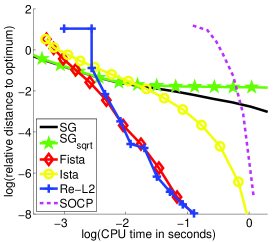
(a) scale: small, regul.: low

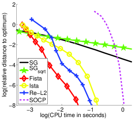
(b) scale: small, regul.: medium

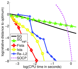
(c) scale: small, regul.: high

Figure 3: Benchmark for solving a least-squares regression problem regularized by the hierarchical norm $\Omega$. The experiment is small scale, $m=256,p=151$, and shows the performances of six optimization methods (see main text for details) for three levels of regularization. The curves represent the relative value of the objective to the optimal value as a function of the computational time in second on a $\log_{10}/\log_{10}$ scale. All reported results are obtained by averaging $5$ runs.

5.2.1 Hierarchical dictionary of natural image patches

In this first benchmark, we consider a least-squares regression problem regularized by $\Omega$ that arises in the context of denoising of natural image patches, as further exposed in Section 5.4. In particular, based on a hierarchical dictionary, we seek to reconstruct noisy $16\!\times\!16$-patches. The dictionary we use is represented on Figure 7. Although the problem involves a small number of variables, i.e., $p=151$ dictionary elements, it has to be solved repeatedly for tens of thousands of patches, at moderate precision. It is therefore crucial to be able to solve this problem quickly and efficiently.

We can draw several conclusions from the results of the simulations reported in Figure 3. First, we observe that in most cases, the accelerated proximal scheme performs better than the other approaches. In addition, unlike FISTA, ISTA seems to suffer in non-sparse scenarios. In the least sparse setting, the reweighted-$\ell_{2}$ scheme is the only method that competes with FISTA. It is however not able to yield truly sparse solutions, and would therefore need a subsequent (somewhat arbitrary) thresholding operation. As expected, the generic techniques such as SG and SOCP do not compete with dedicated algorithms.

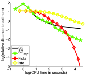
(a) scale: large, regul.: low

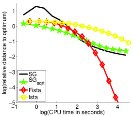
(b) scale: large, regul.: medium

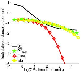
(c) scale: large, regul.: high

Figure 4: Benchmark for solving a large-scale multi-class classification problem for four optimization methods (see details about the datasets and the methods in the main text). Three levels of regularization are considered. The curves represent the relative value of the objective to the optimal value as a function of the computational time in second on a $\log_{10}/\log_{10}$ scale. In the highly regularized setting, tuning the step-size for the subgradient turned out to be difficult, which explains the behavior of SG in the first iterations.

5.2.2 Multi-class classification of cancer diagnosis

The second benchmark explores a different supervised learning setting, where $f$ is no longer the square loss function. The goal is to demonstrate that our optimization tools apply in various scenarios, beyond traditional sparse approximation problems. To this end, we consider a gene expression dataset in the context of cancer diagnosis. More precisely, we focus on a multi-class classification problem where the number $m$ of samples to be classified is small compared to the number $p$ of gene expressions that characterize these samples. Each atom thus corresponds to a gene expression across the $m$ samples, whose class labels are recorded in the vector ${\mathbf{x}}$ in $\mathbb{R}^{m}$.

The dataset contains $m=308$ samples, $p=30\,017$ variables and $26$ classes. In addition, the data exhibit highly-correlated dictionary elements. Inspired by Kim and Xing (2010), we build the tree-structured set of groups $\mathcal{G}$ using Ward’s hierarchical clustering Johnson (1967) on the gene expressions. The norm $\Omega$ built in this way aims at capturing the hierarchical structure of gene expression networks Kim and Xing (2010).

Instead of the square loss function, we consider the multinomial logistic loss function that is better suited to deal with multi-class classification problems (see, e.g., Hastie et al., 2009). As a direct consequence, algorithms whose applicability crucially depends on the choice of the loss function $f$ are removed from the benchmark. This is the case with reweighted-$\ell_{2}$ schemes that do not have closed-form updates anymore. Importantly, the choice of the multinomial logistic loss function leads to an optimization problem over a matrix with dimensions $p$ times the number of classes (i.e., a total of $30\,017\times 26\approx 780\,000$ variables). Also, due to scalability issues, generic interior point solvers could not be considered here.

The results in Figure 4 highlight that the accelerated proximal scheme performs overall better that the two other methods. Again, it is important to note that both proximal algorithms yield sparse solutions, which is not the case for SG.

5.3 Denoising with Tree-Structured Wavelets

We demonstrate in this section how a tree-structured sparse regularization can improve classical wavelet representation, and how our method can be used to efficiently solve the corresponding large-scale optimization problems. We consider two wavelet orthonormal bases, Haar and Daubechies3 (see Mallat, 1999), and choose a classical quad-tree structure on the coefficients, which has notably proven to be useful for image compression problems Baraniuk (1999). This experiment follows the approach of Zhao et al. (2009) who used the same tree-structured regularization in the case of small one-dimensional signals, and the approach of Baraniuk et al. (2010) and Huang et al. (2009) images where images were reconstructed from compressed sensing measurements with a hierarchical nonconvex penalty.

We compare the performance for image denoising of both nonconvex and convex approaches. Specifically, we consider the following formulation

$$\min_{{\boldsymbol{\alpha}}\in\mathbb{R}^{m}}\frac{1}{2}\|{\mathbf{x}}-{\mathbf{D}}{\boldsymbol{\alpha}}\|_{2}^{2}+\lambda\psi({\boldsymbol{\alpha}})=\min_{{\boldsymbol{\alpha}}\in\mathbb{R}^{m}}\frac{1}{2}\|{\mathbf{D}}^{\top}{\mathbf{x}}-{\boldsymbol{\alpha}}\|_{2}^{2}+\lambda\psi({\boldsymbol{\alpha}}),$$

where ${\mathbf{D}}$ is one of the orthonormal wavelet basis mentioned above, ${\mathbf{x}}$ is the input noisy image, ${\mathbf{D}}{\boldsymbol{\alpha}}$ is the estimate of the denoised image, and $\psi$ is a sparsity-inducing regularization. Note that in this case, $m=p$. We first consider classical settings where $\psi$ is either the $\ell_{1}$-norm— this leads to the wavelet soft-thresholding method of Donoho and Johnstone (1995)— or the $\ell_{0}$-pseudo-norm, whose solution can be obtained by hard-thresholding (see Mallat, 1999). Then, we consider the convex tree-structured regularization $\Omega$ defined as a sum of $\ell_{2}$-norms ($\ell_{\infty}$-norms), which we denote by $\Omega_{\ell_{2}}$ (respectively $\Omega_{\ell_{\infty}}$). Since the basis is here orthonormal, solving the corresponding decomposition problems amounts to computing a single instance of the proximal operator. As a result, when $\psi$ is $\Omega_{\ell_{2}}$, we use Algorithm 3 and for $\Omega_{\ell_{\infty}}$, Algorithm 2 is applied. Finally, we consider the nonconvex tree-structured regularization used by Baraniuk et al. (2010) denoted here by $\ell_{0}^{\text{tree}}$, which we have presented in Eq. (4); the implementation details for $\ell_{0}^{\text{tree}}$ can be found in Appendix A.

		Haar
	$\sigma$	$\ell_{0}\;[0.0012]$	$\ell_{0}^{\text{tree}}\;[0.0098]$	$\ell_{1}\;[0.0016]$	$\Omega_{\ell_{2}}\;[0.0125]$	$\Omega_{\ell_{\infty}}\;[0.0221]$
PSNR	$5$	34.48	34.78	35.52	35.89	35.79
	$10$	29.63	30.24	30.74	31.40	31.23
	$25$	24.44	25.27	25.30	26.41	26.14
	$50$	21.53	22.37	20.42	23.41	23.05
	$100$	19.27	20.09	19.43	20.97	20.58
IPSNR	$5$	-	$.30\pm.23$	$1.04\pm.31$	$\mathbf{1.41\pm.45}$	$1.31\pm.41$
	$10$	-	$.60\pm.24$	$1.10\pm.22$	$\mathbf{1.76\pm.26}$	$1.59\pm.22$
	$25$	-	$.83\pm.13$	$.86\pm.35$	$\mathbf{1.96\pm.22}$	$1.69\pm.21$
	$50$	-	$.84\pm.18$	$.46\pm.28$	$\mathbf{1.87\pm.20}$	$1.51\pm.20$
	$100$	-	$.82\pm.14$	$.15\pm.23$	$\mathbf{1.69\pm.19}$	$1.30\pm.19$
		Daub3
	$\sigma$	$\ell_{0}\;[0.0013]$	$\ell_{0}^{\text{tree}}\;[0.0099]$	$\ell_{1}\;[0.0017]$	$\Omega_{\ell_{2}}\;[0.0129]$	$\Omega_{\ell_{\infty}}\;[0.0204]$
PSNR	$5$	34.64	34.95	35.74	36.14	36.00
	$10$	30.03	30.63	31.10	31.79	31.56
	$25$	25.04	25.84	25.76	26.90	26.54
	$50$	22.09	22.90	22.42	23.90	23.41
	$100$	19.56	20.45	19.67	21.40	20.87
IPSNR	$5$	-	$.31\pm.21$	$1.10\pm.23$	$\mathbf{1.49\pm.34}$	$1.36\pm.31$
	$10$	-	$.60\pm.16$	$1.06\pm.25$	$\mathbf{1.76\pm.19}$	$1.53\pm.17$
	$25$	-	$.80\pm.10$	$.71\pm.28$	$\mathbf{1.85\pm.17}$	$1.50\pm.18$
	$50$	-	$.81\pm.15$	$.33\pm.24$	$\mathbf{1.80\pm.11}$	$1.33\pm.12$
	$100$	-	$.89\pm.13$	$0.11\pm.24$	$\mathbf{1.82\pm.24}$	$1.30\pm.17$

Table 1: Top part of the tables: Average PSNR measured for the denoising of $12$ standard images, when the wavelets are Haar or Daubechies3 wavelets (see Mallat, 1999), for two nonconvex approaches ($\ell_{0}$ and $\ell_{0}^{\text{tree}}$) and three different convex regularizations—that is, the $\ell_{1}$-norm, the tree-structured sum of $\ell_{2}$-norms ($\Omega_{\ell_{2}}$), and the tree-structured sum of $\ell_{\infty}$-norms ($\Omega_{\ell_{\infty}}$). Best results for each level of noise and each wavelet type are in bold. Bottom part of the tables: Average improvement in PSNR with respect to the $\ell_{0}$ nonconvex method (the standard deviations are computed over the 12 images). CPU times (in second) averaged over all images and noise realizations are reported in brackets next to the names of the methods they correspond to.

Compared to Zhao et al. (2009), the novelty of our approach is essentially to be able to solve efficiently and exactly large-scale instances of this problem. We use $12$ classical standard test images, and generate noisy versions of them corrupted by a white Gaussian noise of variance $\sigma$. For each image, we test several values of $\lambda=2^{\frac{i}{4}}\sigma\sqrt{\log{m}}$, with $i$ taken in a specific range. We then keep the parameter $\lambda$ giving the best reconstruction error. The factor $\sigma\sqrt{\log{m}}$ is a classical heuristic for choosing a reasonable regularization parameter (see Mallat, 1999). We provide reconstruction results in terms of PSNR in Table 1. We report in this table the results when $\Omega$ is chosen to be a sum of $\ell_{2}$-norms or $\ell_{\infty}$-norms with weights $\omega_{g}$ all equal to one. Each experiment was run $5$ times with different noise realizations. In every setting, we observe that the tree-structured norm significantly outperforms the $\ell_{1}$-norm and the nonconvex approaches. We also present a visual comparison on two images on Figure 5, showing that the tree-structured norm reduces visual artefacts (these artefacts are better seen by zooming on a computer screen). The wavelet transforms in our experiments are computed with the matlabPyrTools software.

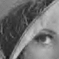
(a) Lena, $\sigma=25$, $\ell_{1}$

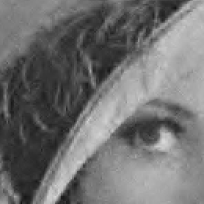
(b) Lena, $\sigma=25$, $\Omega_{\ell_{2}}$

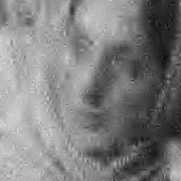
(c) Barb., $\sigma=50$, $\ell_{1}$

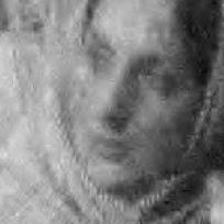
(d) Barb., $\sigma=50$, $\Omega_{\ell_{2}}$

Figure 5: Visual comparison between the wavelet shrinkage model with the $\ell_{1}$-norm and the tree-structured model, on cropped versions of the images Lena and Barb.. Haar wavelets are used.

This experiment does of course not provide state-of-the-art results for image denoising (see Mairal et al., 2009b, and references therein), but shows that the tree-structured regularization significantly improves the reconstruction quality for wavelets. In this experiment the convex setting $\Omega_{\ell_{2}}$ and $\Omega_{\ell_{\infty}}$ also outperforms the nonconvex one $\ell_{0}^{\text{tree}}$. We also note that the speed of our approach makes it scalable to real-time applications. Solving the proximal problem for an image with $m=512\times 512=262\,144$ pixels takes approximately $0.013$ seconds on a single core of a 3.07GHz CPU if $\Omega$ is a sum of ${\ell_{2}}$-norms, and $0.02$ seconds when it is a sum of $\ell_{\infty}$-norms. By contrast, unstructured approaches have a speed-up factor of about 7-8 with respect to the tree-structured methods.

5.4 Dictionaries of Natural Image Patches

This experiment studies whether a hierarchical structure can help dictionaries for denoising natural image patches, and in which noise regime the potential gain is significant. We aim at reconstructing corrupted patches from a test set, after having learned dictionaries on a training set of non-corrupted patches. Though not typical in machine learning, this setting is reasonable in the context of images, where lots of non-corrupted patches are easily available.

noise	50 %	60 %	70 %	80 %	90 %
flat	$19.3\pm 0.1$	$26.8\pm 0.1$	$36.7\pm 0.1$	$50.6\pm 0.0$	$72.1\pm 0.0$
tree	$18.6\pm 0.1$	$25.7\pm 0.1$	$35.0\pm 0.1$	$48.0\pm 0.0$	$65.9\pm 0.3$

Table 2: Quantitative results of the reconstruction task on natural image patches. First row: percentage of missing pixels. Second and third rows: mean square error multiplied by $100$, respectively for classical sparse coding, and tree-structured sparse coding.

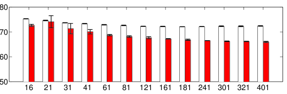
Figure 6: Mean square error multiplied by $100$ obtained with $13$ structures with error bars, sorted by number of dictionary elements from $16$ to $401$. Red plain bars represents the tree-structured dictionaries. White bars correspond to the flat dictionary model containing the same number of dictionary as the tree-structured one. For readability purpose, the $y$-axis of the graph starts at $50$.

We extracted $100\,000$ patches of size $m=8\times 8$ pixels from the Berkeley segmentation database of natural images Martin et al. (2001), which contains a high variability of scenes. We then split this dataset into a training set ${\mathbf{X}}_{tr}$, a validation set ${\mathbf{X}}_{val}$, and a test set ${\mathbf{X}}_{te}$, respectively of size $50\,000$, $25\,000$, and $25\,000$ patches. All the patches are centered and normalized to have unit $\ell_{2}$-norm.

For the first experiment, the dictionary ${\mathbf{D}}$ is learned on ${\mathbf{X}}_{tr}$ using the formulation of Eq. (10), with $\mu=0$ for ${\mathcal{D}_{\mu}}$ as defined in Eq. (11). The validation and test sets are corrupted by removing a certain percentage of pixels, the task being to reconstruct the missing pixels from the known pixels. We thus introduce for each element ${\mathbf{x}}$ of the validation/test set, a vector ${\bf\tilde{x}}$, equal to ${\mathbf{x}}$ for the known pixel values and $0$ otherwise. Similarly, we define ${\bf\tilde{D}}$ as the matrix equal to ${\mathbf{D}}$, except for the rows corresponding to missing pixel values, which are set to $0$. By decomposing ${\bf\tilde{x}}$ on ${\bf\tilde{D}}$, we obtain a sparse code ${\boldsymbol{\alpha}}$, and the estimate of the reconstructed patch is defined as ${\mathbf{D}}{\boldsymbol{\alpha}}$. Note that this procedure assumes that we know which pixel is missing and which is not for every element ${\mathbf{x}}$.

The parameters of the experiment are the regularization parameter $\lambda_{tr}$ used during the training step, the regularization parameter $\lambda_{te}$ used during the validation/test step, and the structure of the tree. For every reported result, these parameters were selected by taking the ones offering the best performance on the validation set, before reporting any result from the test set. The values for the regularization parameters $\lambda_{tr},\lambda_{te}$ were selected on a logarithmic scale $\{2^{-10},2^{-9},\ldots,2^{2}\}$, and then further refined on a finer logarithmic scale with multiplicative increments of $2^{-1/4}$. For simplicity, we chose arbitrarily to use the $\ell_{\infty}$-norm in the structured norm $\Omega$, with all the weights equal to one. We tested $21$ balanced tree structures of depth $3$ and $4$, with different branching factors $p_{1},p_{2},\ldots,p_{d-1}$, where $d$ is the depth of the tree and $p_{k}$, $k\in\{1,\ldots,d-1\}$ is the number of children for the nodes at depth $k$. The branching factors tested for the trees of depth $3$ where $p_{1}\in\{5,10,20,40,60,80,100\}$, $p_{2}\in\{2,3\}$, and for trees of depth $4$, $p_{1}\in\{5,10,20,40\}$, $p_{2}\in\{2,3\}$ and $p_{3}=2$, giving $21$ possible structures associated with dictionaries with at most $401$ elements. For each tree structure, we evaluated the performance obtained with the tree-structured dictionary along with a non-structured dictionary containing the same number of elements. These experiments were carried out four times, each time with a different initialization, and with a different noise realization.

Quantitative results are reported in Table 2. For all fractions of missing pixels considered, the tree-structured dictionary outperforms the “unstructured one”, and the most significant improvement is obtained in the noisiest setting. Note that having more dictionary elements is worthwhile when using the tree structure. To study the influence of the chosen structure, we report in Figure 6 the results obtained with the $13$ tested structures of depth $3$, along with those obtained with unstructured dictionaries containing the same number of elements, when $90\%$ of the pixels are missing. For each dictionary size, the tree-structured dictionary significantly outperforms the unstructured one. An example of a learned tree-structured dictionary is presented on Figure 7. Dictionary elements naturally organize in groups of patches, often with low frequencies near the root of the tree, and high frequencies near the leaves.

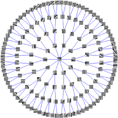
Figure 7: Learned dictionary with a tree structure of depth $5$. The root of the tree is in the middle of the figure. The branching factors are $p_{1}=10$, $p_{2}=2$, $p_{3}=2$, $p_{4}=2$. The dictionary is learned on $50,000$ patches of size $16\times 16$ pixels.

5.5 Text Documents

This last experimental section shows that our approach can also be applied to model text corpora. The goal of probabilistic topic models is to find a low-dimensional representation of a collection of documents, where the representation should provide a semantic description of the collection. Approaching the problem in a parametric Bayesian framework, latent Dirichlet allocation (LDA) Blei et al. (2003) model documents, represented as vectors of word counts, as a mixture of a predefined number of latent topics that are distributions over a fixed vocabulary. LDA is fundamentally a matrix factorization problem: Buntine (2002) shows that LDA can be interpreted as a Dirichlet-multinomial counterpart of factor analysis. The number of topics is usually small compared to the size of the vocabulary (e.g., 100 against $10\,000$), so that the topic proportions of each document provide a compact representation of the corpus. For instance, these new features can be used to feed a classifier in a subsequent classification task. We similarly use our dictionary learning approach to find low-dimensional representations of text corpora.

Suppose that the signals ${\mathbf{X}}=[{\mathbf{x}}^{1},\dots,{\mathbf{x}}^{n}]$ in $\mathbb{R}^{m\times n}$ are each the bag-of-word representation of each of $n$ documents over a vocabulary of $m$ words, the $k$-th component of ${\mathbf{x}}^{i}$ standing for the frequency of the $k$-th word in the document $i$. If we further assume that the entries of ${\mathbf{D}}$ and ${\mathbf{A}}$ are nonnegative, and that the dictionary elements ${\mathbf{d}}^{j}$ have unit $\ell_{1}$-norm, the decomposition $({\mathbf{D}},{\mathbf{A}})$ can be interpreted as the parameters of a topic-mixture model. The regularization $\Omega$ induces the organization of these topics on a tree, so that, if a document involves a certain topic, then all ancestral topics in the tree are also present in the topic decomposition. Since the hierarchy is shared by all documents, the topics at the top of the tree participate in every decomposition, and should therefore gather the lexicon which is common to all documents. Conversely, the deeper the topics in the tree, the more specific they should be. An extension of LDA to model topic hierarchies was proposed by Blei et al. (2010), who introduced a non-parametric Bayesian prior over trees of topics and modelled documents as convex combinations of topics selected along a path in the hierarchy. We plan to compare our approach with this model in future work.

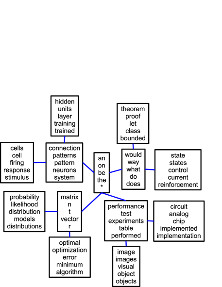
Figure 8: Example of a topic hierarchy estimated from 1714 NIPS proceedings papers (from 1988 through 1999). Each node corresponds to a topic whose 5 most important words are displayed. Single characters such as $n,t,r$ are part of the vocabulary and often appear in NIPS papers, and their place in the hierarchy is semantically relevant to children topics.

Visualization of NIPS proceedings.

We qualitatively illustrate our approach on the NIPS proceedings from 1988 through 1999 Griffiths and Steyvers (2004). After removing words appearing fewer than 10 times, the dataset is composed of 1714 articles, with a vocabulary of 8274 words. As explained above, we consider $\mathcal{D}_{1}^{+}$ and take $\mathcal{A}$ to be $\mathbb{R}^{p\times n}_{+}$. Figure 8 displays an example of a learned dictionary with 13 topics, obtained by using the $\ell_{\infty}$-norm in $\Omega$ and selecting manually $\lambda\!=\!2^{-15}$. As expected and similarly to Blei et al. (2010), we capture the stopwords at the root of the tree, and topics reflecting the different subdomains of the conference such as neurosciences, optimization or learning theory.

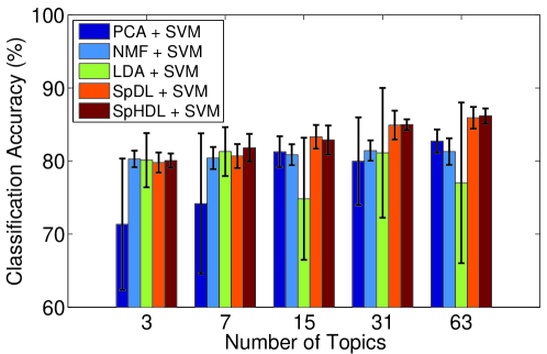
Figure 9: Binary classification of two newsgroups: classification accuracy for different dimensionality reduction techniques coupled with a linear SVM classifier. The bars and the errors are respectively the mean and the standard deviation, based on 10 random splits of the dataset. Best seen in color.

Posting classification.

We now consider a binary classification task of $n$ postings from the 20 Newsgroups data set. We learn to discriminate between the postings from the two newsgroups alt.atheism and talk.religion.misc, following the setting of Lacoste-Julien et al. (2008) and Zhu et al. (2009). After removing words appearing fewer than 10 times and standard stopwords, these postings form a data set of 1425 documents over a vocabulary of 13312 words. We compare different dimensionality reduction techniques that we use to feed a linear SVM classifier, i.e., we consider (i) LDA, with the code from Blei et al. (2003), (ii) principal component analysis (PCA), (iii) nonnegative matrix factorization (NMF), (iv) standard sparse dictionary learning (denoted by SpDL) and (v) our sparse hierarchical approach (denoted by SpHDL). Both SpDL and SpHDL are optimized over $\mathcal{D}_{1}^{+}$ and $\mathcal{A}\!=\!\mathbb{R}^{p\times n}_{+}$, with the weights $\omega_{g}$ equal to 1. We proceed as follows: given a random split into a training/test set of $1\,000/425$ postings, and given a number of topics $p$ (also the number of components for PCA, NMF, SpDL and SpHDL), we train an SVM classifier based on the low-dimensional representation of the postings. This is performed on a training set of $1\,000$ postings, where the parameters, $\lambda\!\in\!\{2^{-26},\dots,2^{-5}\}$ and/or $C_{\text{svm}}\!\in\!\{4^{-3},\dots,4^{1}\}$ are selected by 5-fold cross-validation. We report in Figure 9 the average classification scores on the test set of 425 postings, based on 10 random splits, for different number of topics. Unlike the experiment on image patches, we consider only complete binary trees with depths in $\{1,\dots,5\}$. The results from Figure 9 show that SpDL and SpHDL perform better than the other dimensionality reduction techniques on this task. As a baseline, the SVM classifier applied directly to the raw data (the 13312 words) obtains a score of $90.9\!\pm\!1.1$, which is better than all the tested methods, but without dimensionality reduction (as already reported by Blei et al., 2003). Moreover, the error bars indicate that, though nonconvex, SpDL and SpHDL do not seem to suffer much from instability issues. Even if SpDL and SpHDL perform similarly, SpHDL has the advantage to provide a more interpretable topic mixture in terms of hierarchy, which standard unstructured sparse coding does not.

6 Discussion

We have applied hierarchical sparse coding in various settings, with fixed/learned dictionaries, and based on different types of data, namely, natural images and text documents. A line of research to pursue is to develop other optimization tools for structured norms with general overlapping groups. For instance, Mairal et al. (2010b) have used network flow optimization techniques for that purpose, and Bach (2010) submodular function optimization. This framework can also be used in the context of hierarchical kernel learning Bach (2008), where we believe that our method can be more efficient than existing ones.

This work establishes a connection between dictionary learning and probabilistic topic models, which should prove fruitful as the two lines of work have focused on different aspects of the same unsupervised learning problem: Our approach is based on convex optimization tools, and provides experimentally more stable data representations. Moreover, it can be easily extended with the same tools to other types of structures corresponding to other norms Jenatton et al. (2009); Jacob et al. (2009). It should be noted, however, that, unlike some Bayesian methods, dictionary learning by itself does not provide mechanisms for the automatic selection of model hyper-parameters (such as the dictionary size or the topology of the tree). An interesting common line of research to pursue could be the supervised design of dictionaries, which has been proved useful in the two frameworks Mairal et al. (2009a); Bradley and Bagnell (2009); Blei and McAuliffe (2008).

Acknowledgments

This paper was partially supported by grants from the Agence Nationale de la Recherche (MGA Project) and from the European Research Council (SIERRA Project 239993). The authors would like to thank Jean Ponce for interesting discussions and suggestions for improving this manuscript. They also would like to thank Volkan Cevher for pointing out links between our approach and nonconvex tree-structured regularization and for insightful discussions. Finally, we thank the reviewers for their constructive and helpful comments.

A Links with Tree-Structured Nonconvex Regularization

We present in this section an algorithm introduced by Donoho (1997) in the more general context of approximation from dyadic partitions (see Section 6 in Donoho, 1997). This algorithm solves the following problem

$$\min_{{\mathbf{v}}\in\mathbb{R}^{p}}\frac{1}{2}\|{\mathbf{u}}-{\mathbf{v}}\|_{2}^{2}+\lambda\sum_{g\in\mathcal{G}}\delta^{g}({\mathbf{v}}),$$ (12)

where the ${\mathbf{u}}$ in $\mathbb{R}^{p}$ is given, $\lambda$ is a regularization parameter, $\mathcal{G}$ is a set of tree-structured groups in the sense of definition 1, and the functions $\delta^{g}$ are defined as in Eq. (4)—that is, $\delta^{g}({\mathbf{v}})=1$ if there exists $j$ in $g$ such that ${\mathbf{v}}_{j}\neq 0$, and $0$ otherwise. This problem can be viewed as a proximal operator for the nonconvex regularization $\sum_{g\in\mathcal{G}}\delta^{g}({\mathbf{v}})$. As we will show, it can be solved efficiently, and in fact it can be used to obtain approximate solutions of the nonconvex problem presented in Eq. (1), or to solve tree-structured wavelet decompositions as done by Baraniuk et al. (2010).

We now briefly show how to derive the dynamic programming approach introduced by Donoho (1997). Given a group $g$ in $\mathcal{G}$, we use the same notations $\text{root}(g)$ and children(g) introduced in Section 3.5. It is relatively easy to show that finding a solution of Eq. (12) amounts to finding the support $S\subseteq\{1,\ldots,p\}$ of its solution and that the problem can be equivalently rewritten

$$\min_{S\subseteq\{1,\ldots,p\}}-\frac{1}{2}\|{\mathbf{u}}_{S}\|_{2}^{2}+\lambda\sum_{g\in\mathcal{G}}\delta^{g}(S),$$ (13)

with the abusive notation $\delta^{g}(S)=1$ if $g\cap S\neq\emptyset$ and $0$ otherwise. We now introduce the quantity

$$\psi_{g}(S)\stackrel{{\scriptstyle\vartriangle}}{{=}}\begin{cases}0&~{}\text{if}~{}g\cap S=\emptyset\\ -\frac{1}{2}\|{\mathbf{u}}_{\text{root}(g)}\|_{2}^{2}+\lambda+\sum_{h\in\text{children}(g)}\psi_{h}(S)&~{}\text{otherwise}.\end{cases}$$

After a few computations, solving Eq. (13) can be shown to be equivalent to minimizing $\psi_{g_{0}}(S)$ where $g_{0}$ is the root of the tree. It is then easy to prove that for any group $g$ in $\mathcal{G}$, we have

$$\min_{S\subseteq\{1,\ldots,p\}}\psi_{g}(S)=\min\Big{(}0,-\frac{1}{2}\|{\mathbf{u}}_{\text{root}(g)}\|_{2}^{2}+\lambda+\sum_{h\in\text{children}(g)}\min_{S^{\prime}\subseteq\{1,\ldots,p\}}\psi_{h}(S^{\prime})\Big{)},$$

which leads to the following dynamic programming approach presented in Algorithm 4.

Algorithm 4 Computation of the Proximal Operator for the Nonconvex Approach

  Inputs: ${\mathbf{u}}\in\mathbb{R}^{p}$, a tree-structured set of groups $\mathcal{G}$ and $g_{0}$ (root of the tree).

  Outputs: ${\mathbf{v}}$ (primal solution).

  Initialization: ${\mathbf{v}}\leftarrow{\mathbf{u}}$.

  Call recursiveThresholding($g_{0}$).

Procedure recursiveThresholding($g$)

1:  $\eta\leftarrow\min\Big{(}0,-\frac{1}{2}\|{\mathbf{u}}_{\text{root}(g)}\|_{2}^{2}+\lambda+\sum_{h\in\text{children}(g)}\text{{recursiveThresholding}}(h)\Big{)}$.

2:  if  $\eta=0$  then

3:     ${\mathbf{v}}_{g}\leftarrow 0$.

4:  end if

5:  Return $\eta$.

This algorithm shares several conceptual links with Algorithm 2 and 3. It traverses the tree in the same order, has a complexity in $O(p)$, and it can be shown that the whole procedure actually performs a sequence of thresholding operations on the variable ${\mathbf{v}}$.

B Proofs

We gather here the proofs of the technical results of the paper.

B.1 Proof of Lemma 1

Proof  The proof relies on tools from conic duality Boyd and Vandenberghe (2004). Let us introduce the cone $\mathcal{C}\stackrel{{\scriptstyle\vartriangle}}{{=}}\{({\mathbf{v}},z)\in\mathbb{R}^{p+1};\ \|{\mathbf{v}}\|\leq z\}$ and its dual counterpart $\mathcal{C^{\ast}}\stackrel{{\scriptstyle\vartriangle}}{{=}}\{({\boldsymbol{\xi}},\tau)\in\mathbb{R}^{p+1};\ \|{\boldsymbol{\xi}}\|_{\ast}\leq\tau\}$. These cones induce generalized inequalities for which Lagrangian duality also applies. We refer the interested readers to Boyd and Vandenberghe (2004) for further details.

We can rewrite problem (7) as

$$\min_{{\mathbf{v}}\in\mathbb{R}^{p},{\mathbf{z}}\in\mathbb{R}^{|\mathcal{G}|}}\frac{1}{2}\|{\mathbf{u}}-{\mathbf{v}}\|_{2}^{2}+\lambda\sum_{g\in\mathcal{G}}\omega_{g}z_{g},\ \text{such that}\ ({\mathbf{v}}_{{{\scriptscriptstyle\mid}g}},z_{g})\in\mathcal{C},\ \forall g\in\mathcal{G},$$

by introducing the primal variables ${\mathbf{z}}=(z_{g})_{g\in\mathcal{G}}\in\mathbb{R}^{|\mathcal{G}|}$, with the additional $|\mathcal{G}|$ conic constraints $({\mathbf{v}}_{{{\scriptscriptstyle\mid}g}},z_{g})\in\mathcal{C}$, for $g\in\mathcal{G}$.

This primal problem is convex and satisfies Slater’s conditions for generalized conic inequalities (i.e., existence of a feasible point in the interior of the domain), which implies that strong duality holds Boyd and Vandenberghe (2004). We now consider the Lagrangian $\mathcal{L}$ defined as

$$\mathcal{L}({\mathbf{v}},{\mathbf{z}},{\boldsymbol{\tau}},{\boldsymbol{\xi}})=\frac{1}{2}\|{\mathbf{u}}-{\mathbf{v}}\|_{2}^{2}+\lambda\sum_{g\in\mathcal{G}}\omega_{g}z_{g}-\sum_{g\in\mathcal{G}}\binom{z_{g}}{{\mathbf{v}}_{{{\scriptscriptstyle\mid}g}}}^{\top}\binom{\tau_{g}}{{\boldsymbol{\xi}}^{g}},$$

with the dual variables ${\boldsymbol{\tau}}=(\tau_{g})_{g\in\mathcal{G}}$ in $\mathbb{R}^{|\mathcal{G}|}$, and ${\boldsymbol{\xi}}=({\boldsymbol{\xi}}^{g})_{g\in\mathcal{G}}$ in $\mathbb{R}^{p\times|\mathcal{G}|}$, such that for all $g\in\mathcal{G}$, ${\boldsymbol{\xi}}^{g}_{j}=0\,\mbox{ if }\,j\notin g$ and $({\boldsymbol{\xi}}^{g},\tau_{g})\in\mathcal{C^{\ast}}$.

The dual function is obtained by minimizing out the primal variables. To this end, we take the derivatives of $\mathcal{L}$ with respect to the primal variables ${\mathbf{v}}$ and ${\mathbf{z}}$ and set them to zero, which leads to

$${\mathbf{v}}-{\mathbf{u}}-\sum_{g\in\mathcal{G}}{\boldsymbol{\xi}}^{g}=0\quad\mathrm{and}\quad\forall g\in\mathcal{G},\ \lambda\omega_{g}-\tau_{g}=0.$$

After simplifying the Lagrangian and flipping (without loss of generality) the sign of ${\boldsymbol{\xi}}$, we obtain the dual problem in Eq. (8). We derive the optimality conditions from the Karush–Kuhn–Tucker conditions for generalized conic inequalities Boyd and Vandenberghe (2004). We have that $\{{\mathbf{v}},{\mathbf{z}},{\boldsymbol{\tau}},{\boldsymbol{\xi}}\}$ are optimal if and only if

$$\forall g\in\mathcal{G},z_{g}\tau_{g}-{\mathbf{v}}_{{{\scriptscriptstyle\mid}g}}^{\top}{\boldsymbol{\xi}}^{g} =0,\quad\text{(Complementary slackness)}$$

$$\forall g\in\mathcal{G},({\mathbf{v}}_{{{\scriptscriptstyle\mid}g}},z_{g})\in\mathcal{C}, \forall g\in\mathcal{G},\lambda\omega_{g}-\tau_{g} =0,$$

$$\forall g\in\mathcal{G},({\boldsymbol{\xi}}^{g},\tau_{g})\in\mathcal{C^{\ast}}, {\mathbf{v}}-{\mathbf{u}}+\sum_{g\in\mathcal{G}}{\boldsymbol{\xi}}^{g} =0.$$

Combining the complementary slackness with the definition of the dual norm, we have

$$\forall g\in\mathcal{G},\ z_{g}\tau_{g}={\mathbf{v}}_{{{\scriptscriptstyle\mid}g}}^{\top}{\boldsymbol{\xi}}^{g}\leq\|{\mathbf{v}}_{{{\scriptscriptstyle\mid}g}}\|\|{\boldsymbol{\xi}}^{g}\|_{\ast}.$$

Furthermore, using the fact that $\forall g\in\mathcal{G},\ ({\mathbf{v}}_{{{\scriptscriptstyle\mid}g}},z_{g})\in\mathcal{C}$ and $({\boldsymbol{\xi}}^{g},\tau_{g})=({\boldsymbol{\xi}}^{g},\lambda\omega_{g})\in\mathcal{C^{\ast}}$, we obtain the following chain of inequalities

$$\forall g\in\mathcal{G},\ \lambda z_{g}\omega_{g}={\mathbf{v}}_{{{\scriptscriptstyle\mid}g}}^{\top}{\boldsymbol{\xi}}^{g}\leq\|{\mathbf{v}}_{{{\scriptscriptstyle\mid}g}}\|\|{\boldsymbol{\xi}}^{g}\|_{\ast}\leq z_{g}\|{\boldsymbol{\xi}}^{g}\|_{\ast}\leq\lambda z_{g}\omega_{g},$$

for which equality must hold. In particular, we have ${\mathbf{v}}_{{{\scriptscriptstyle\mid}g}}^{\top}{\boldsymbol{\xi}}^{g}=\|{\mathbf{v}}_{{{\scriptscriptstyle\mid}g}}\|\|{\boldsymbol{\xi}}^{g}\|_{\ast}$ and $z_{g}\|{\boldsymbol{\xi}}^{g}\|_{\ast}=\lambda z_{g}\omega_{g}$. If ${\mathbf{v}}_{{{\scriptscriptstyle\mid}g}}\neq 0$, then $z_{g}$ cannot be equal to zero, which implies in turn that $\|{\boldsymbol{\xi}}^{g}\|_{\ast}=\lambda\omega_{g}$. Eventually, applying Lemma 5 gives the advertised optimality conditions.

Conversely, starting from the optimality conditions of Lemma 1, and making use again of Lemma 5, we can derive the Karush–Kuhn–Tucker conditions displayed above. More precisely, we define for all $g\in\mathcal{G}$,

$$\tau_{g}\stackrel{{\scriptstyle\vartriangle}}{{=}}\lambda\omega_{g}\quad\text{and}\quad z_{g}\stackrel{{\scriptstyle\vartriangle}}{{=}}\|{\mathbf{v}}_{{{\scriptscriptstyle\mid}g}}\|.$$

The only condition that needs to be discussed is the complementary slackness condition. If ${\mathbf{v}}_{{{\scriptscriptstyle\mid}g}}=0$, then it is easily satisfied. Otherwise, combining the definitions of $\tau_{g},\ z_{g}$ and the fact that

$${\mathbf{v}}_{{{\scriptscriptstyle\mid}g}}^{\top}{\boldsymbol{\xi}}^{g}=\|{\mathbf{v}}_{{{\scriptscriptstyle\mid}g}}\|\|{\boldsymbol{\xi}}^{g}\|_{\ast}\ \text{and}\ \|{\boldsymbol{\xi}}^{g}\|_{\ast}=\lambda\omega_{g},$$

we end up with the desired complementary slackness.  

B.2 Optimality condition for the projection on the dual ball

Lemma 5 (Projection on the dual ball)

Let ${\mathbf{w}}\in\mathbb{R}^{p}$ and $t>0$. We have ${\boldsymbol{\kappa}}=\Pi_{\|.\|_{\ast}\leq t}({\mathbf{w}})$ if and only if

$$\begin{cases}\text{if}\ \|{\mathbf{w}}\|_{\ast}\leq t,&{\boldsymbol{\kappa}}={\mathbf{w}},\\ \text{otherwise,}&\|{\boldsymbol{\kappa}}\|_{\ast}=t\ \mbox{ and }\ {\boldsymbol{\kappa}}^{\top}({\mathbf{w}}-{\boldsymbol{\kappa}})=\|{\boldsymbol{\kappa}}\|_{\ast}\|{\mathbf{w}}-{\boldsymbol{\kappa}}\|.\end{cases}$$

Proof  When the vector ${\mathbf{w}}$ is already in the ball of $\|.\|_{\ast}$ with radius $t$, i.e., $\|{\mathbf{w}}\|_{\ast}\leq t$, the situation is simple, since the projection $\Pi_{\|.\|_{\ast}\leq t}({\mathbf{w}})$ obviously gives ${\mathbf{w}}$ itself. On the other hand, a necessary and sufficient optimality condition for having ${\boldsymbol{\kappa}}=\Pi_{\|.\|_{\ast}\leq t}({\mathbf{w}})=\operatornamewithlimits{arg\,min}_{\|{\mathbf{y}}\|_{\ast}\leq t}\|{\mathbf{w}}-{\mathbf{y}}\|_{2}$ is that the residual ${\mathbf{w}}-{\boldsymbol{\kappa}}$ lies in the normal cone of the constraint set Borwein and Lewis (2006), that is, for all ${\mathbf{y}}$ such that $\|{\mathbf{y}}\|_{\ast}\!\leq t$, $({\mathbf{w}}-{\boldsymbol{\kappa}})^{\top}\!({\mathbf{y}}-{\boldsymbol{\kappa}})\!\leq 0$. The displayed result then follows from the definition of the dual norm, namely $\|{\boldsymbol{\kappa}}\|_{\ast}\!=\!\max_{\|{\mathbf{z}}\|\leq 1}{\mathbf{z}}^{\top}{\boldsymbol{\kappa}}$.  

B.3 Proof of Lemma 2

Proof  First, notice that the conclusion ${\boldsymbol{\xi}}^{h}=\Pi_{\|.\|_{\ast}\leq\lambda\omega_{h}}({\mathbf{v}}_{{{\scriptscriptstyle\mid}h}}+{\boldsymbol{\xi}}^{h})$ simply comes from the definition of ${\boldsymbol{\xi}}^{h}$ and ${\mathbf{v}}$, along with the fact that ${\boldsymbol{\xi}}^{g}={\boldsymbol{\xi}}_{{{\scriptscriptstyle\mid}h}}^{g}$ since $g\subseteq h$. We now examine ${\boldsymbol{\xi}}^{g}$.

The proof mostly relies on the optimality conditions characterizing the projection onto a ball of the dual norm $\|\cdot\|_{\ast}$. Precisely, by Lemma 5, we need to show that either

$${\boldsymbol{\xi}}^{g}={\mathbf{u}}_{{{\scriptscriptstyle\mid}g}}-{\boldsymbol{\xi}}_{{{\scriptscriptstyle\mid}g}}^{h},\ \text{if}\ \|{\mathbf{u}}_{{{\scriptscriptstyle\mid}g}}-{\boldsymbol{\xi}}_{{{\scriptscriptstyle\mid}g}}^{h}\|_{\ast}\leq t_{g},$$

or

$$\|{\boldsymbol{\xi}}^{g}\|_{\ast}=t_{g}\ \mbox{ and }\ {\boldsymbol{\xi}}^{g\top}({\mathbf{u}}_{{{\scriptscriptstyle\mid}g}}-{\boldsymbol{\xi}}_{{{\scriptscriptstyle\mid}g}}^{h}-{\boldsymbol{\xi}}^{g})=\|{\boldsymbol{\xi}}^{g}\|_{\ast}\|{\mathbf{u}}_{{{\scriptscriptstyle\mid}g}}-{\boldsymbol{\xi}}_{{{\scriptscriptstyle\mid}g}}^{h}-{\boldsymbol{\xi}}^{g}\|.$$

Note that the feasibility of ${\boldsymbol{\xi}}^{g}$, i.e., $\|{\boldsymbol{\xi}}^{g}\|_{\ast}\leq t_{g}$, holds by definition of $\kappa^{g}$.

Let us first assume that $\|{\boldsymbol{\xi}}^{g}\|_{\ast}<t_{g}$. We necessarily have that ${\mathbf{u}}_{{{\scriptscriptstyle\mid}g}}$ also lies in the interior of the ball of $\|.\|_{\ast}$ with radius $t_{g}$, and it holds that ${\boldsymbol{\xi}}^{g}={\mathbf{u}}_{{{\scriptscriptstyle\mid}g}}$. Since $g\subseteq h$, we have that the vector ${\mathbf{u}}_{{{\scriptscriptstyle\mid}h}}-{\boldsymbol{\xi}}^{g}={\mathbf{u}}_{{{\scriptscriptstyle\mid}h}}-{\mathbf{u}}_{{{\scriptscriptstyle\mid}g}}$ has only zero entries on $g$. As a result, ${\boldsymbol{\xi}}^{h}_{g}=0$ (or equivalently, ${\boldsymbol{\xi}}^{h}_{{\scriptscriptstyle\mid}g}=0$) and we obtain

$${\boldsymbol{\xi}}^{g}={\mathbf{u}}_{{{\scriptscriptstyle\mid}g}}={\mathbf{u}}_{{{\scriptscriptstyle\mid}g}}-{\boldsymbol{\xi}}_{{{\scriptscriptstyle\mid}g}}^{h},$$

which is the desired conclusion. From now on, we assume that $\|{\boldsymbol{\xi}}^{g}\|_{\ast}=t_{g}$. It then remains to show that

$${\boldsymbol{\xi}}^{g\top}({\mathbf{u}}_{{{\scriptscriptstyle\mid}g}}-{\boldsymbol{\xi}}_{{{\scriptscriptstyle\mid}g}}^{h}-{\boldsymbol{\xi}}^{g})=\|{\boldsymbol{\xi}}^{g}\|_{\ast}\|{\mathbf{u}}_{{{\scriptscriptstyle\mid}g}}-{\boldsymbol{\xi}}_{{{\scriptscriptstyle\mid}g}}^{h}-{\boldsymbol{\xi}}^{g}\|.$$

We now distinguish two cases, according to the norm used.

$\ell_{2}$-norm: As a consequence of Lemma 5, the optimality condition reduces to the conditions for equality in the Cauchy-Schwartz inequality, i.e., when the vectors have same signs and are linearly dependent. Applying these conditions to individual projections we get that there exists $\rho_{g},\rho_{h}>0$ such that

$$\rho_{g}{\boldsymbol{\xi}}^{g}={\mathbf{u}}_{{{\scriptscriptstyle\mid}g}}-{\boldsymbol{\xi}}^{g}\quad\mathrm{and}\quad\rho_{h}{\boldsymbol{\xi}}^{h}={\mathbf{u}}_{{{\scriptscriptstyle\mid}h}}-{\boldsymbol{\xi}}^{g}-{\boldsymbol{\xi}}^{h}.$$ (14)

Note that the case $\rho_{h}=0$ leads to ${\mathbf{u}}_{{{\scriptscriptstyle\mid}h}}-{\boldsymbol{\xi}}^{g}-{\boldsymbol{\xi}}^{h}=0$, and therefore ${\mathbf{u}}_{{{\scriptscriptstyle\mid}g}}-{\boldsymbol{\xi}}^{g}-{\boldsymbol{\xi}}_{{{\scriptscriptstyle\mid}g}}^{h}=0$ since $g\subseteq h$, which directly yields the result. The case $\rho_{g}=0$ implies ${\mathbf{u}}_{{{\scriptscriptstyle\mid}g}}-{\boldsymbol{\xi}}^{g}=0$ and therefore ${\boldsymbol{\xi}}_{{{\scriptscriptstyle\mid}g}}^{h}=0$, yielding the result as well. Now, we can therefore assume $\rho_{h}>0$ and $\rho_{g}>0$. From the first equality of (14), we have ${\boldsymbol{\xi}}^{g}={\boldsymbol{\xi}}^{g}_{{\scriptscriptstyle\mid}g}$ since $(\rho_{g}+1){\boldsymbol{\xi}}^{g}={\mathbf{u}}_{{{\scriptscriptstyle\mid}g}}$. Further using the fact that $g\subseteq h$ in the second equality of  (14), we obtain

$$(\rho_{h}+1){\boldsymbol{\xi}}^{h}_{{\scriptscriptstyle\mid}g}={\mathbf{u}}_{{\scriptscriptstyle\mid}g}-{\boldsymbol{\xi}}^{g}=\rho_{g}{\boldsymbol{\xi}}^{g}.$$

This implies that ${\mathbf{u}}_{{{\scriptscriptstyle\mid}g}}-{\boldsymbol{\xi}}^{g}-{\boldsymbol{\xi}}_{{{\scriptscriptstyle\mid}g}}^{h}=\rho_{g}{\boldsymbol{\xi}}^{g}-\frac{\rho_{g}}{\rho_{h}+1}{\boldsymbol{\xi}}^{g}$, which eventually leads to

$${\boldsymbol{\xi}}^{g}=\frac{\rho_{h}+1}{\rho_{g}\rho_{h}}({\mathbf{u}}_{{{\scriptscriptstyle\mid}g}}-{\boldsymbol{\xi}}^{g}-{\boldsymbol{\xi}}_{{{\scriptscriptstyle\mid}g}}^{h}).$$

The desired conclusion follows ${\boldsymbol{\xi}}^{g\top}({\mathbf{u}}_{{{\scriptscriptstyle\mid}g}}-{\boldsymbol{\xi}}^{g}-{\boldsymbol{\xi}}_{{{\scriptscriptstyle\mid}g}}^{h})=\|{\boldsymbol{\xi}}^{g}\|_{2}\|{\mathbf{u}}_{{{\scriptscriptstyle\mid}g}}-{\boldsymbol{\xi}}^{g}-{\boldsymbol{\xi}}_{{{\scriptscriptstyle\mid}g}}^{h}\|_{2}.$

$\ell_{\infty}$-norm: In this case, the optimality corresponds to the conditions for equality in the $\ell_{\infty}$-$\ell_{1}$ Hölder inequality. Specifically, ${\boldsymbol{\xi}}^{g}=\Pi_{\|.\|_{\ast}\leq t_{g}}({\mathbf{u}}_{{{\scriptscriptstyle\mid}g}})$ holds if and only if for all ${\boldsymbol{\xi}}^{g}_{j}\neq 0,j\in g$, we have

$${\mathbf{u}}_{j}-{\boldsymbol{\xi}}^{g}_{j}=\|{\mathbf{u}}_{{{\scriptscriptstyle\mid}g}}-{\boldsymbol{\xi}}^{g}\|_{\infty}\operatorname{sign}({\boldsymbol{\xi}}^{g}_{j}).$$

Looking at the same condition for ${\boldsymbol{\xi}}^{h}$, we have that ${\boldsymbol{\xi}}^{h}=\Pi_{\|.\|_{\ast}\leq t_{h}}\big{(}{\mathbf{u}}_{{{\scriptscriptstyle\mid}h}}-{\boldsymbol{\xi}}_{g}\big{)}$ holds if and only if for all ${\boldsymbol{\xi}}^{h}_{j}\neq 0,j\in h$, we have

$${\mathbf{u}}_{j}-{\boldsymbol{\xi}}^{g}_{j}-{\boldsymbol{\xi}}^{h}_{j}=\|{\mathbf{u}}_{{{\scriptscriptstyle\mid}h}}-{\boldsymbol{\xi}}^{g}-{\boldsymbol{\xi}}^{h}\|_{\infty}\operatorname{sign}({\boldsymbol{\xi}}^{h}_{j}).$$

From those relationships we notably deduce that for all $j\in g$ such that ${\boldsymbol{\xi}}^{g}_{j}\neq 0$, $\operatorname{sign}({\boldsymbol{\xi}}^{g}_{j})=\operatorname{sign}({\mathbf{u}}_{j})=\operatorname{sign}({\boldsymbol{\xi}}^{h}_{j})=\operatorname{sign}({\mathbf{u}}_{j}-{\boldsymbol{\xi}}^{g}_{j})=\operatorname{sign}({\mathbf{u}}_{j}-{\boldsymbol{\xi}}^{g}_{j}-{\boldsymbol{\xi}}^{h}_{j})$. Let $j\in g$ such that ${\boldsymbol{\xi}}^{g}_{j}\neq 0$. At this point, using the equalities we have just presented,

$$|{\mathbf{u}}_{j}-{\boldsymbol{\xi}}^{g}_{j}-{\boldsymbol{\xi}}^{h}_{j}|=\left\{\begin{array}[]{ll}\|{\mathbf{u}}_{{{\scriptscriptstyle\mid}g}}-{\boldsymbol{\xi}}^{g}\|_{\infty}&\text{if}~{}{\boldsymbol{\xi}}^{h}_{j}=0\\ \|{\mathbf{u}}_{{{\scriptscriptstyle\mid}h}}-{\boldsymbol{\xi}}^{g}-{\boldsymbol{\xi}}^{h}\|_{\infty}&\text{if}~{}{\boldsymbol{\xi}}^{h}_{j}\neq 0.\end{array}\right.$$

Since $\|{\mathbf{u}}_{{{\scriptscriptstyle\mid}g}}-{\boldsymbol{\xi}}^{g}\|_{\infty}\geq\|{\mathbf{u}}_{{{\scriptscriptstyle\mid}g}}-{\boldsymbol{\xi}}^{g}-{\boldsymbol{\xi}}_{{{\scriptscriptstyle\mid}g}}^{h}\|_{\infty}$ (which can be shown using the sign equalities above), and $\|{\mathbf{u}}_{{{\scriptscriptstyle\mid}h}}-{\boldsymbol{\xi}}^{g}-{\boldsymbol{\xi}}^{h}\|_{\infty}\geq\|{\mathbf{u}}_{{{\scriptscriptstyle\mid}g}}-{\boldsymbol{\xi}}^{g}-{\boldsymbol{\xi}}_{{{\scriptscriptstyle\mid}g}}^{h}\|_{\infty}$ (since $g\subseteq h$), we have

$$\|{\mathbf{u}}_{{{\scriptscriptstyle\mid}g}}-{\boldsymbol{\xi}}^{g}-{\boldsymbol{\xi}}_{{{\scriptscriptstyle\mid}g}}^{h}\|_{\infty}\geq|{\mathbf{u}}_{j}-{\boldsymbol{\xi}}^{g}_{j}-{\boldsymbol{\xi}}^{h}_{j}|\geq\|{\mathbf{u}}_{{{\scriptscriptstyle\mid}g}}-{\boldsymbol{\xi}}^{g}-{\boldsymbol{\xi}}_{{{\scriptscriptstyle\mid}g}}^{h}\|_{\infty},$$

and therefore for all ${\boldsymbol{\xi}}^{g}_{j}\neq 0$, $j\in g$, we have ${\mathbf{u}}_{j}-{\boldsymbol{\xi}}^{g}_{j}-{\boldsymbol{\xi}}^{h}_{j}=\|{\mathbf{u}}_{{{\scriptscriptstyle\mid}g}}-{\boldsymbol{\xi}}^{g}-{\boldsymbol{\xi}}_{{{\scriptscriptstyle\mid}g}}^{h}\|_{\infty}\operatorname{sign}({\boldsymbol{\xi}}^{g}_{j}),$ which yields the result.  

B.4 Proof of Lemma 4

Proof  Notice first that the procedure computeSqNorm is called exactly once for each group $g$ in $\mathcal{G}$, computing a set of scalars $(\rho_{g})_{g\in\mathcal{G}}$ in an order which is compatible with the convergence in one pass of Algorithm 1—that is, the children of a node are processed prior to the node itself. Following such an order, the update of the group $g$ in the original Algorithm 1 computes the variable ${\boldsymbol{\xi}}^{g}$ which updates implicitly the primal variable as follows

$${\mathbf{v}}_{{{\scriptscriptstyle\mid}g}}\leftarrow\big{(}1-\frac{\lambda\omega_{g}}{\|{\mathbf{v}}_{{{\scriptscriptstyle\mid}g}}\|_{2}}\big{)}_{+}\,{\mathbf{v}}_{{{\scriptscriptstyle\mid}g}}.$$

It is now possible to show by induction that for all group $g$ in $\mathcal{G}$, after a call to the procedure computeSqNorm($g$), the auxiliary variable $\eta_{g}$ takes the value $\|{\mathbf{v}}_{{{\scriptscriptstyle\mid}g}}\|_{2}^{2}$ where ${\mathbf{v}}$ has the same value as during the iteration $g$ of Algorithm 1. Therefore, after calling the procedure computeSqNorm($g_{0}$), where $g_{0}$ is the root of the tree, the values $\rho_{g}$ correspond to the successive scaling factors of the variable ${\mathbf{v}}_{{{\scriptscriptstyle\mid}g}}$ obtained during the execution of Algorithm 1. After having computed all the scaling factors $\rho_{g}$, $g\in\mathcal{G}$, the procedure recursiveScaling ensures that each variable $j$ in $\{1,\ldots,p\}$ is scaled by the product of all the $\rho_{h}$, where $h$ is an ancestor of the variable $j$.

The complexity of the algorithm is easy to characterize: Each procedure computeSqNorm and recursiveScaling is called $p$ times, each call for a group $g$ has a constant number of operations plus as many operations as the number of children of $p$. Since each child can be called at most one time, the total number of operation of the algorithm is $O(p)$.  

B.5 Sign conservation by projection

The next lemma specifies a property for projections when $\|.\|$ is further assumed to be a $\ell_{q}$-norm (with $q\geq 1$). We recall that in that case, $\|.\|_{\ast}$ is simply the $\ell_{q^{\prime}}$-norm, with $q^{\prime}=(1-1/q)^{-1}$.

Lemma 6 (Projection on the dual ball and sign property)

Let ${\mathbf{w}}\in\mathbb{R}^{p}$ and $t>0$. Let us assume that $\|.\|$ is a $\ell_{q}$-norm (with $q\geq 1$). Consider also a diagonal matrix ${\mathbf{S}}\in\mathbb{R}^{p\times p}$ whose diagonal entries are in $\{-1,1\}$. We have $\Pi_{\|.\|_{\ast}\leq t}({\mathbf{w}})={\mathbf{S}}\Pi_{\|.\|_{\ast}\leq t}({\mathbf{S}}{\mathbf{w}}).$

Proof  Let us consider ${\boldsymbol{\kappa}}=\Pi_{\|.\|_{\ast}\leq t}({\mathbf{w}})$. Using essentially the same argument as in the proof of Lemma 5, we have for all ${\mathbf{y}}$ such that $\|{\mathbf{y}}\|_{q^{\prime}}\!\leq t$, $({\mathbf{w}}-{\boldsymbol{\kappa}})^{\top}\!({\mathbf{y}}-{\boldsymbol{\kappa}})\!\leq 0$. Noticing that ${\mathbf{S}}^{\top}{\mathbf{S}}={\mathbf{I}}$ and $\|{\mathbf{y}}\|_{q^{\prime}}=\|{\mathbf{S}}{\mathbf{y}}\|_{q^{\prime}}$, we further obtain $({\mathbf{S}}{\mathbf{w}}-{\mathbf{S}}{\boldsymbol{\kappa}})^{\top}\!({\mathbf{y}}^{\prime}-{\mathbf{S}}{\boldsymbol{\kappa}})\!\leq 0$ for all ${\mathbf{y}}^{\prime}$ with $\|{\mathbf{y}}^{\prime}\|_{q^{\prime}}\!\leq t$. This implies in turn that ${\mathbf{S}}\Pi_{\|.\|_{\ast}\leq t}({\mathbf{w}})=\Pi_{\|.\|_{\ast}\leq t}({\mathbf{S}}{\mathbf{w}})$, which is equivalent to the advertised conclusion.  
Based on this lemma, note that we can assume without loss of generality that the vector we want to project (in this case, ${\mathbf{w}}$) has only nonnegative entries. Indeed, it is sufficient to store beforehand the signs of that vector, compute the projection of the vector with nonnegative entries, and assign the stored signs to the result of the projection.

B.6 Non-negativity constraint for the proximal operator

The next lemma shows how we can easily add a non-negativity constraint on the proximal operator when the norm $\Omega$ is absolute (Stewart and Sun, 1990, Definition 1.2), that is, a norm for which the relation $\Omega({\mathbf{u}})\leq\Omega({\mathbf{w}})$ holds for any two vectors ${\mathbf{w}}$ and ${\mathbf{u}}\in\mathbb{R}^{p}$ such that $|{\mathbf{u}}_{j}|\leq|{\mathbf{w}}_{j}|$ for all $j$.

Lemma 7 (Non-negativity constraint for the proximal operator)

Let ${\boldsymbol{\kappa}}\in\mathbb{R}^{p}$ and $\lambda>0$. Consider an absolute norm $\Omega$. We have

$$\operatornamewithlimits{arg\,min}_{{\mathbf{z}}\in\mathbb{R}^{p}}\Big{[}\frac{1}{2}\!\|[{\boldsymbol{\kappa}}]_{+}\!-{\mathbf{z}}\|_{2}^{2}+\lambda\Omega({\mathbf{z}})\Big{]}=\operatornamewithlimits{arg\,min}_{{\mathbf{z}}\in\mathbb{R}^{p}_{+}}\Big{[}\frac{1}{2}\!\|{\boldsymbol{\kappa}}\!-{\mathbf{z}}\|_{2}^{2}+\lambda\Omega({\mathbf{z}})\Big{]}.$$ (15)

Proof  Let us denote by $\hat{{\mathbf{z}}}^{+}$ and $\hat{{\mathbf{z}}}$ the unique solutions of the left- and right-hand side of (15) respectively. Consider the normal cone ${\mathcal{N}}_{\mathbb{R}^{p}_{+}}({\mathbf{z}}_{0})$ of $\mathbb{R}^{p}_{+}$ at the point ${\mathbf{z}}_{0}$ (Borwein and Lewis, 2006) and decompose ${\boldsymbol{\kappa}}$ into its positive and negative parts, ${\boldsymbol{\kappa}}=[{\boldsymbol{\kappa}}]_{+}+[{\boldsymbol{\kappa}}]_{-}$. We can now write down the optimality conditions for the two convex problems above (Borwein and Lewis, 2006): $\hat{{\mathbf{z}}}^{+}$ is optimal if and only if there exists ${\mathbf{w}}\in\partial\Omega(\hat{{\mathbf{z}}}^{+})$ such that $\hat{{\mathbf{z}}}^{+}-[{\boldsymbol{\kappa}}]_{+}+\lambda{\mathbf{w}}=\mathbf{0}.$ Similarly, $\hat{{\mathbf{z}}}$ is optimal if and only if there exists $({\mathbf{s}},{\mathbf{u}})\in\partial\Omega(\hat{{\mathbf{z}}})\times{\mathcal{N}}_{\mathbb{R}^{p}_{+}}(\hat{{\mathbf{z}}})$ such that $\hat{{\mathbf{z}}}-{\boldsymbol{\kappa}}+\lambda{\mathbf{s}}+{\mathbf{u}}=\mathbf{0}.$ We now prove that $[{\boldsymbol{\kappa}}]_{-}={\boldsymbol{\kappa}}-[{\boldsymbol{\kappa}}]_{+}$ belongs to ${\mathcal{N}}_{\mathbb{R}^{p}_{+}}(\hat{{\mathbf{z}}}^{+})$. We proceed by contradiction. Let us assume that there exists ${\mathbf{z}}\in\mathbb{R}^{p}_{+}$ such that $[{\boldsymbol{\kappa}}]_{-}^{\top}({\mathbf{z}}-\hat{{\mathbf{z}}}^{+})>0$. This implies that there exists $j\in\{1,\dots,p\}$ for which $[{\boldsymbol{\kappa}}_{j}]_{-}<0$ and ${\mathbf{z}}_{j}-\hat{{\mathbf{z}}}^{+}_{j}<0$. In other words, we have $0\leq{\mathbf{z}}_{j}={\mathbf{z}}_{j}-[{\boldsymbol{\kappa}}_{j}]_{+}<\hat{{\mathbf{z}}}^{+}_{j}=\hat{{\mathbf{z}}}^{+}_{j}-[{\boldsymbol{\kappa}}_{j}]_{+}$. With the assumption made on $\Omega$ and replacing $\hat{{\mathbf{z}}}^{+}_{j}$ by ${\mathbf{z}}_{j}$, we have found a solution to the left-hand side of (15) with a stricly smaller cost function than the one evaluated at $\hat{{\mathbf{z}}}^{+}$, hence the contradiction. Putting the pieces together, we now have

$$\hat{{\mathbf{z}}}^{+}-[{\boldsymbol{\kappa}}]_{+}+\lambda{\mathbf{w}}=\hat{{\mathbf{z}}}^{+}-{\boldsymbol{\kappa}}+\lambda{\mathbf{w}}+[{\boldsymbol{\kappa}}]_{-}=\mathbf{0},\ \text{with}\ ({\mathbf{w}},[{\boldsymbol{\kappa}}]_{-})\in\partial\Omega(\hat{{\mathbf{z}}}^{+})\times{\mathcal{N}}_{\mathbb{R}^{p}_{+}}(\hat{{\mathbf{z}}}^{+}),$$

which shows that $\hat{{\mathbf{z}}}^{+}$ is the solution of the right-hand side of (15).  

C Counterexample for $\ell_{q}$-norms, with $q\notin\{1,2,\infty\}$.

The result we have proved in Proposition 1 in the specific setting where $\|.\|$ is the $\ell_{2}$- or $\ell_{\infty}$-norm does not hold more generally for $\ell_{q}$-norms, when $q$ is not in $\{1,2,\infty\}$. Let $q>1$ satisfying this condition. We denote by $q^{\prime}\stackrel{{\scriptstyle\vartriangle}}{{=}}(1-q^{-1})^{-1}$ the norm parameter dual to $q$. We keep the same notation as in Lemma 2 and assume from now on that $\|{\mathbf{u}}_{{{\scriptscriptstyle\mid}g}}\|_{q^{\prime}}>t_{g}$ and $\|{\mathbf{u}}_{{{\scriptscriptstyle\mid}h}}\|_{q^{\prime}}>t_{g}+t_{h}$. These two inequalities guarantee that the vectors ${\mathbf{u}}_{{{\scriptscriptstyle\mid}g}}$ and ${\mathbf{u}}_{{{\scriptscriptstyle\mid}h}}-{\boldsymbol{\xi}}^{g}$ do not lie in the interior of the $\ell_{q^{\prime}}$-norm balls, of respective radius $t_{g}$ and $t_{h}$.

We show in this section that there exists a setting for which the conclusion of Lemma 2 does not hold anymore. We first focus on a necessary condition of Lemma 2:

Lemma 8 (Necessary condition of Lemma 2)

Let $\|.\|$ be a $\ell_{q}$-norm, with $q\notin\{1,2,\infty\}$. If the conclusion of Lemma 2 holds, then the vectors ${\boldsymbol{\xi}}_{{{\scriptscriptstyle\mid}g}}^{g}$ and ${\boldsymbol{\xi}}_{{{\scriptscriptstyle\mid}g}}^{h}$ are linearly dependent.

Proof  According to our assumptions on ${\mathbf{u}}_{{{\scriptscriptstyle\mid}g}}$ and ${\mathbf{u}}_{{{\scriptscriptstyle\mid}h}}-{\boldsymbol{\xi}}^{g}$, we have that $\|{\boldsymbol{\xi}}^{g}\|_{q^{\prime}}=t_{g}$ and $\|{\boldsymbol{\xi}}^{h}\|_{q^{\prime}}=t_{h}$. In this case, we can apply the second optimality conditions of Lemma 5, which states that equality holds in the $\ell_{q}$-$\ell_{q^{\prime}}$ Hölder inequality. As a result, there exists $\rho_{g},\rho_{h}>0$ such that for all $j$ in $g$:

$$|{\boldsymbol{\xi}}_{j}^{g}|^{q^{\prime}}=\rho_{g}|{\mathbf{u}}_{j}-{\boldsymbol{\xi}}_{j}^{g}|^{q}\quad\mathrm{and}\quad|{\boldsymbol{\xi}}_{j}^{h}|^{q^{\prime}}=\rho_{h}|{\mathbf{u}}_{j}-{\boldsymbol{\xi}}_{j}^{g}-{\boldsymbol{\xi}}_{j}^{h}|^{q}.$$ (16)

If the conclusion of Lemma 2 holds—that is, we have ${\boldsymbol{\xi}}^{g}=\Pi_{\|.\|_{\ast}\leq t_{g}}({\mathbf{u}}_{{{\scriptscriptstyle\mid}g}}-{\boldsymbol{\xi}}_{{{\scriptscriptstyle\mid}g}}^{h})$, notice that it is not possible to have the following scenarios, as proved below by contradiction:

• If $\|{\mathbf{u}}_{{{\scriptscriptstyle\mid}g}}-{\boldsymbol{\xi}}_{{{\scriptscriptstyle\mid}g}}^{h}\|_{q^{\prime}}<t_{g}$, then we would have ${\boldsymbol{\xi}}^{g}={\mathbf{u}}_{{{\scriptscriptstyle\mid}g}}-{\boldsymbol{\xi}}_{{{\scriptscriptstyle\mid}g}}^{h}$, which is impossible since $\|{\boldsymbol{\xi}}^{g}\|_{q^{\prime}}=t_{g}$.

• If $\|{\mathbf{u}}_{{{\scriptscriptstyle\mid}g}}-{\boldsymbol{\xi}}_{{{\scriptscriptstyle\mid}g}}^{h}\|_{q^{\prime}}=t_{g}$, then we would have for all $j$ in $g$, $|{\boldsymbol{\xi}}_{j}^{h}|^{q^{\prime}}=\rho_{h}|{\mathbf{u}}_{j}-{\boldsymbol{\xi}}_{j}^{g}-{\boldsymbol{\xi}}_{j}^{h}|^{q}=0$, which implies that ${\boldsymbol{\xi}}_{{{\scriptscriptstyle\mid}g}}^{h}=0$ and $\|{\mathbf{u}}_{{{\scriptscriptstyle\mid}g}}\|_{q^{\prime}}=t_{g}$. This is impossible since we assumed $\|{\mathbf{u}}_{{{\scriptscriptstyle\mid}g}}\|_{q^{\prime}}>t_{g}$.

We therefore have $\|{\mathbf{u}}_{{{\scriptscriptstyle\mid}g}}-{\boldsymbol{\xi}}_{{{\scriptscriptstyle\mid}g}}^{h}\|_{q^{\prime}}>t_{g}$ and using again the second optimality conditions of Lemma 5, there exists $\rho>0$ such that for all $j$ in $g$, $|{\boldsymbol{\xi}}_{j}^{g}|^{q^{\prime}}=\rho|{\mathbf{u}}_{j}-{\boldsymbol{\xi}}_{j}^{g}-{\boldsymbol{\xi}}_{j}^{h}|^{q}$. Combined with the previous relation on ${\boldsymbol{\xi}}_{{{\scriptscriptstyle\mid}g}}^{h}$, we obtain for all $j$ in $g$, $|{\boldsymbol{\xi}}_{j}^{g}|^{q^{\prime}}=\frac{\rho}{\rho_{h}}|{\boldsymbol{\xi}}_{j}^{h}|^{q^{\prime}}.$ Since we can assume without loss of generality that ${\mathbf{u}}$ only has nonnegative entries (see Lemma 6), the vectors ${\boldsymbol{\xi}}^{g}$ and ${\boldsymbol{\xi}}^{h}$ can also be assumed to have nonnegative entries, hence the desired conclusion.  
We need another intuitive property of the projection $\Pi_{\|.\|_{\ast}\leq t}$ to derive our counterexample:

Lemma 9 (Order-preservation by projection)

Let $\|.\|$ be a $\ell_{q}$-norm, with $q\notin\{1,\infty\}$ and $q^{\prime}\stackrel{{\scriptstyle\vartriangle}}{{=}}1/(1-q^{-1})$. Let us consider the vectors ${\boldsymbol{\kappa}},{\mathbf{w}}\in\mathbb{R}^{p}$ such that ${\boldsymbol{\kappa}}=\Pi_{\|.\|_{\ast}\leq t}({\mathbf{w}})=\operatornamewithlimits{arg\,min}_{\|{\mathbf{y}}\|_{q^{\prime}}\leq t}\|{\mathbf{y}}-{\mathbf{w}}\|_{2},$ with the radius $t$ satisfying $\|{\mathbf{w}}\|_{q^{\prime}}>t$. If we have ${\mathbf{w}}_{i}<{\mathbf{w}}_{j}$ for some $(i,j)$ in $\{1,\dots,p\}^{2}$, then it also holds that ${\boldsymbol{\kappa}}_{i}<{\boldsymbol{\kappa}}_{j}$.

Proof  Let us first notice that given the assumption on $t$, we have $\|{\boldsymbol{\kappa}}\|_{q^{\prime}}=t$. The Lagrangian $\mathcal{L}$ associated with the convex minimization problem underlying the definition of $\Pi_{\|.\|_{\ast}\leq t}$ can be written as

$$\mathcal{L}({\mathbf{y}},\alpha)=\frac{1}{2}\|{\mathbf{y}}-{\mathbf{w}}\|^{2}_{2}+\alpha\big{[}\|{\mathbf{y}}\|^{q^{\prime}}_{q^{\prime}}-t^{q^{\prime}}\big{]},\ \text{with the Lagrangian parameter}\ \alpha\geq 0.$$

At optimality, the stationarity condition for ${\boldsymbol{\kappa}}$ leads to

$$\forall\ j\in\{1,\dots,p\},\ {\boldsymbol{\kappa}}_{j}-{\mathbf{w}}_{j}+\alpha{q^{\prime}}|{\boldsymbol{\kappa}}_{j}|^{q^{\prime}-1}=0.$$

We can assume without loss of generality that ${\mathbf{w}}$ only has nonnegative entries (see Lemma 6). Since the components of ${\boldsymbol{\kappa}}$ and ${\mathbf{w}}$ have the same signs (see Lemma 6), we therefore have $|{\boldsymbol{\kappa}}_{j}|={\boldsymbol{\kappa}}_{j}\geq 0$, for all $j$ in $\{1,\dots,p\}$. Note that $\alpha$ cannot be equal to zero because of $\|{\boldsymbol{\kappa}}\|_{q^{\prime}}=t<\|{\mathbf{w}}\|_{q^{\prime}}$.

Let us consider the continuously differentiable function $\varphi_{w}:\kappa\mapsto\kappa-w+\alpha q^{\prime}\kappa^{q^{\prime}-1}$ defined on $(0,\infty)$. Since $\varphi_{w}(0)=-w<0$, $\lim_{\kappa\to\infty}\varphi_{w}(\kappa)=\infty$ and $\varphi_{w}$ is strictly nondecreasing, there exists a unique $\kappa^{\ast}_{w}>0$ such that $\varphi_{w}(\kappa^{\ast}_{w})=0$. If we now take $w<v$, we have

$$\varphi_{v}(\kappa^{\ast}_{w})=\varphi_{w}(\kappa^{\ast}_{w})+w-v=w-v<0=\varphi_{v}(\kappa^{\ast}_{v}).$$

With $\varphi_{v}$ being strictly nondecreasing, we thus obtain $\kappa^{\ast}_{w}<\kappa^{\ast}_{v}$. The desired conclusion stems from the application of the previous result to the stationarity condition of ${\boldsymbol{\kappa}}$.  

Based on the two previous lemmas, we are now in position to present our counterexample:

Proposition 2 (Counterexample)

Let $\|.\|$ be a $\ell_{q}$-norm, with $q\notin\{1,2,\infty\}$ and $q^{\prime}\stackrel{{\scriptstyle\vartriangle}}{{=}}1/(1-q^{-1})$. Let us consider $\mathcal{G}=\{g,h\}$, with $g\subseteq h\subseteq\{1,\dots,p\}$ and $|g|>1$. Let ${\mathbf{u}}$ be a vector in $\mathbb{R}^{p}$ that has at least two different nonzero entries in $g$, i.e., there exists $(i,j)$ in $g\times g$ such that $0<|{\mathbf{u}}_{i}|<|{\mathbf{u}}_{j}|$. Let us consider the successive projections

$${\boldsymbol{\xi}}^{g}\stackrel{{\scriptstyle\vartriangle}}{{=}}\Pi_{\|.\|_{\ast}\leq t_{g}}({\mathbf{u}}_{{{\scriptscriptstyle\mid}g}})~{}\text{ and }~{}{\boldsymbol{\xi}}^{h}\stackrel{{\scriptstyle\vartriangle}}{{=}}\Pi_{\|.\|_{\ast}\leq t_{h}}({\mathbf{u}}_{{{\scriptscriptstyle\mid}h}}-{\boldsymbol{\xi}}^{g})$$

with $t_{g},t_{h}>0$ satisfying $\|{\mathbf{u}}_{{{\scriptscriptstyle\mid}g}}\|_{q^{\prime}}>t_{g}$ and $\|{\mathbf{u}}_{{{\scriptscriptstyle\mid}h}}\|_{q^{\prime}}>t_{g}+t_{h}$. Then, the conclusion of Lemma 2 does not hold.

Proof  We apply the same rationale as in the proof of Lemma 9. Writing the stationarity conditions for ${\boldsymbol{\xi}}^{g}$ and ${\boldsymbol{\xi}}^{h}$, we have for all $j$ in $g$

$${\boldsymbol{\xi}}_{j}^{g}+\alpha q^{\prime}({\boldsymbol{\xi}}_{j}^{g})^{q^{\prime}-1}-{\mathbf{u}}_{j}=0,\quad\mathrm{and}\quad{\boldsymbol{\xi}}_{j}^{h}+\beta q^{\prime}({\boldsymbol{\xi}}_{j}^{h})^{q^{\prime}-1}-({\mathbf{u}}_{j}-{\boldsymbol{\xi}}_{j}^{g})=0,$$ (17)

with Lagrangian parameters $\alpha,\beta>0$. We now proceed by contradiction and assume that ${\boldsymbol{\xi}}^{g}=\Pi_{\|.\|_{\ast}\leq t_{g}}({\mathbf{u}}_{{{\scriptscriptstyle\mid}g}}-{\boldsymbol{\xi}}_{{{\scriptscriptstyle\mid}g}}^{h}).$ According to Lemma 8, there exists $\rho>0$ such that for all $j$ in $g$, ${\boldsymbol{\xi}}_{j}^{h}=\rho{\boldsymbol{\xi}}_{j}^{g}.$ If we combine the previous relations on ${\boldsymbol{\xi}}^{g}$ and ${\boldsymbol{\xi}}^{h}$, we obtain for all $j$ in $g$,

$${\boldsymbol{\xi}}_{j}^{g}=C({\boldsymbol{\xi}}_{j}^{g})^{q^{\prime}-1},\ \text{with}\ C\stackrel{{\scriptstyle\vartriangle}}{{=}}\frac{q^{\prime}(\alpha-\beta\rho^{q^{\prime}-1})}{\rho}.$$

If $C<0$, then we have a contradiction, since the entries of ${\boldsymbol{\xi}}^{g}$ and ${\mathbf{u}}_{{{\scriptscriptstyle\mid}g}}$ have the same signs. Similarly, the case $C=0$ leads a contradiction, since we would have ${\mathbf{u}}_{{{\scriptscriptstyle\mid}g}}=0$ and $\|{\mathbf{u}}_{{{\scriptscriptstyle\mid}g}}\|_{q^{\prime}}>t_{g}$. As a consequence, it follows that $C>0$ and for all $j$ in $g$, ${\boldsymbol{\xi}}_{j}^{g}=\exp\big{\{}\frac{\log(C)}{2-q^{\prime}}\big{\}},$ which means that all the entries of the vector ${\boldsymbol{\xi}}_{g}^{g}$ are identical. Using Lemma 9, since there exists $(i,j)\in g\times g$ such that ${\mathbf{u}}_{i}<{\mathbf{u}}_{j}$, we also have ${\boldsymbol{\xi}}_{i}^{g}<{\boldsymbol{\xi}}_{j}^{g}$, which leads to a contradiction.

References

- Aharon et al. (2006) M. Aharon, M. Elad, and A. M. Bruckstein. The K-SVD: An algorithm for designing of overcomplete dictionaries for sparse representations. IEEE Transactions on Signal Processing, 54(11):4311–4322, 2006.
- Ahuja et al. (1993) R. K. Ahuja, T. L. Magnanti, and J. Orlin. Network Flows. Prentice Hall, 1993.
- Bach (2008) F. Bach. Exploring large feature spaces with hierarchical multiple kernel learning. In Advances in Neural Information Processing Systems, 2008.
- Bach (2010) F. Bach. Structured sparsity-inducing norms through submodular functions. In Advances in Neural Information Processing Systems, 2010.
- Bach et al. (2011) F. Bach, R. Jenatton, J. Mairal, and G. Obozinski. Convex optimization with sparsity-inducing norms. In Optimization for Machine Learning. MIT Press, 2011. To appear.
- Baraniuk (1999) R. Baraniuk. Optimal tree approximation with wavelets. Wavelet Applications in Signal and Image Processing VII, 3813:206214, 1999.
- Baraniuk et al. (2002) R. G. Baraniuk, R. A. DeVore, G. Kyriazis, and X. M. Yu. Near best tree approximation. Advances in Computational Mathematics, 16(4):357–373, 2002.
- Baraniuk et al. (2010) R. G. Baraniuk, V. Cevher, M. F. Duarte, and C. Hegde. Model-based compressive sensing. IEEE Transactions on Information Theory, 56:1982–2001, 2010.
- Beck and Teboulle (2009) A. Beck and M. Teboulle. A fast iterative shrinkage-thresholding algorithm for linear inverse problems. SIAM Journal on Imaging Sciences, 2(1):183–202, 2009.
- Becker et al. (2009) S. Becker, J. Bobin, and E. Candes. NESTA: A Fast and Accurate First-order Method for Sparse Recovery. Technical report, Preprint arXiv:0904.3367, 2009.
- Bengio (2009) Y. Bengio. Learning deep architectures for AI. Foundations and Trends in Machine Learning, 2(1), 2009.
- Bertsekas (1999) D. P. Bertsekas. Nonlinear programming. Athena Scientific, 1999.
- Bickel et al. (2009) P. Bickel, Y. Ritov, and A. Tsybakov. Simultaneous analysis of Lasso and Dantzig selector. Annals of Statistics, 37(4):1705–1732, 2009.
- Blei and McAuliffe (2008) D. Blei and J. McAuliffe. Supervised topic models. In Advances in Neural Information Processing Systems, 2008.
- Blei et al. (2003) D. Blei, A. Ng, and M. Jordan. Latent dirichlet allocation. Journal of Machine Learning Research, 3:993–1022, 2003.
- Blei et al. (2010) D. Blei, T. L. Griffiths, and M. I. Jordan. The nested chinese restaurant process and bayesian nonparametric inference of topic hierarchies. Journal of the ACM, 57(2):1–30, 2010.
- Borwein and Lewis (2006) J. M. Borwein and A. S. Lewis. Convex Analysis and Nonlinear Optimization: Theory and Examples. Springer, 2006.
- Boyd and Vandenberghe (2004) S. P. Boyd and L. Vandenberghe. Convex Optimization. Cambridge University Press, 2004.
- Bradley and Bagnell (2009) D. M. Bradley and J. A. Bagnell. Differentiable sparse coding. In Advances in Neural Information Processing Systems, 2009.
- Brucker (1984) P. Brucker. An O(n) algorithm for quadratic knapsack problems. Operations Research Letters, 3:163–166, 1984.
- Buntine (2002) W. L. Buntine. Variational Extensions to EM and Multinomial PCA. In Proceedings of the European Conference on Machine Learning (ECML), 2002.
- Chen et al. (1998) S. S. Chen, D. L. Donoho, and M. A. Saunders. Atomic decomposition by basis pursuit. SIAM Journal on Scientific Computing, 20(1):33–61, 1998.
- Chen et al. (2010) X. Chen, Q. Lin, S. Kim, J. Peña, J. G. Carbonell, and E. P. Xing. An efficient proximal-gradient method for single and multi-task regression with structured sparsity. Technical report, Preprint arXiv:1005.4717, 2010.
- Coifman and Donoho (1995) R. R. Coifman and D. L. Donoho. Translation-invariant de-noising. Lectures notes in statistics, pages 125–125, 1995.
- Combettes and Pesquet (2010) P. L. Combettes and J.-C. Pesquet. Proximal splitting methods in signal processing. In Fixed-Point Algorithms for Inverse Problems in Science and Engineering. Springer, 2010.
- Crouse et al. (1998) M. Crouse, R. D. Nowak, and R. G. Baraniuk. Wavelet-based statistical signal processing using hidden Markov models. IEEE Transactions on Signal Processing, 46(4):886–902, 1998.
- Donoho (1997) D. L. Donoho. CART and best-ortho-basis: a connection. Annals of Statistics, pages 1870–1911, 1997.
- Donoho and Johnstone (1995) D. L. Donoho and I. M. Johnstone. Adapting to unknown smoothness via wavelet shrinkage. Journal of the American Statistical Association, 90(432), 1995.
- Duchi and Singer (2009) J. Duchi and Y. Singer. Efficient online and batch learning using forward backward splitting. Journal of Machine Learning Research, 10:2899–2934, 2009.
- Efron et al. (2004) B. Efron, T. Hastie, I. Johnstone, and R. Tibshirani. Least angle regression. Annals of Statistics, 32(2):407–451, 2004.
- Elad and Aharon (2006) M. Elad and M. Aharon. Image denoising via sparse and redundant representations over learned dictionaries. IEEE Transactions on Image Processing, 54(12):3736–3745, December 2006.
- Friedman et al. (2010) J. Friedman, T. Hastie, and R. Tibshirani. A note on the group lasso and a sparse group lasso. Technical report, Preprint arXiv:1001.0736, 2010.
- Griffiths and Steyvers (2004) T. L. Griffiths and M. Steyvers. Finding scientific topics. Proceedings of the National Academy of Sciences, 101(Suppl 1):5228, 2004.
- Hastie et al. (2009) T. Hastie, R. Tibshirani, and J. Friedman. The Elements of Statistical Learning: Data Mining, Inference, and Prediction, Second Edition. Springer, 2009.
- He and Carin (2009) L. He and L. Carin. Exploiting structure in wavelet-based Bayesian compressive sensing. IEEE Transactions on Signal Processing, 57:3488–3497, 2009.
- Hu et al. (2009) C. Hu, J. T. Kwok, and W. Pan. Accelerated gradient methods for stochastic optimization and online learning. In Advances in Neural Information Processing Systems, 2009.
- Huang et al. (2009) J. Huang, T. Zhang, and D. Metaxas. Learning with structured sparsity. In Proceedings of the International Conference on Machine Learning (ICML), 2009.
- Jacob et al. (2009) L. Jacob, G. Obozinski, and J.-P. Vert. Group Lasso with overlaps and graph Lasso. In Proceedings of the International Conference on Machine Learning (ICML), 2009.
- Jenatton et al. (2009) R. Jenatton, J.-Y. Audibert, and F. Bach. Structured variable selection with sparsity-inducing norms. Technical report, Preprint arXiv:0904.3523, 2009.
- Jenatton et al. (2010) R. Jenatton, J. Mairal, G. Obozinski, and F. Bach. Proximal methods for sparse hierarchical dictionary learning. In Proceedings of the International Conference on Machine Learning (ICML), 2010.
- Johnson (1967) S. C. Johnson. Hierarchical clustering schemes. Psychometrika, 32(3):241–254, 1967.
- Kim and Xing (2010) S. Kim and E. P. Xing. Tree-guided group Lasso for multi-task regression with structured sparsity. In Proceedings of the International Conference on Machine Learning (ICML), 2010.
- Lacoste-Julien et al. (2008) S. Lacoste-Julien, F. Sha, and M. I. Jordan. DiscLDA: Discriminative learning for dimensionality reduction and classification. In Advances in Neural Information Processing Systems, 2008.
- Lee and Seung (1999) D. D. Lee and H. S. Seung. Learning the parts of objects by non-negative matrix factorization. Nature, 401(6755):788–791, 1999.
- Lee et al. (2007) H. Lee, A. Battle, R. Raina, and A. Y. Ng. Efficient sparse coding algorithms. In Advances in Neural Information Processing Systems, 2007.
- Maculan and Galdino de Paula (1989) N. Maculan and J. R. G. Galdino de Paula. A linear-time median-finding algorithm for projecting a vector on the simplex of Rn. Operations Research Letters, 8(4):219–222, 1989.
- Mairal et al. (2009a) J. Mairal, F. Bach, J. Ponce, G. Sapiro, and A. Zisserman. Supervised dictionary learning. In Advances in Neural Information Processing Systems, 2009a.
- Mairal et al. (2009b) J. Mairal, F. Bach, J. Ponce, G. Sapiro, and A. Zisserman. Non-local sparse models for image restoration. In Proceedings of the IEEE International Conference on Computer Vision (ICCV), 2009b.
- Mairal et al. (2010a) J. Mairal, F. Bach, J. Ponce, and G. Sapiro. Online learning for matrix factorization and sparse coding. Journal of Machine Learning Research, 11(1):19–60, 2010a.
- Mairal et al. (2010b) J. Mairal, R. Jenatton, G. Obozinski, and F. Bach. Network flow algorithms for structured sparsity. In Advances in Neural Information Processing Systems, 2010b.
- Mallat (1999) S. G. Mallat. A wavelet tour of signal processing. Academic Press, 1999.
- Martin et al. (2001) D. Martin, C. Fowlkes, D. Tal, and J. Malik. A database of human segmented natural images and its application to evaluating segmentation algorithms and measuring ecological statistics. In Proceedings of the IEEE International Conference on Computer Vision (ICCV), 2001.
- Micchelli et al. (2010) C. A. Micchelli, J. M. Morales, and M. Pontil. A family of penalty functions for structured sparsity. In Advances in Neural Information Processing Systems, 2010.
- Moreau (1962) J. J. Moreau. Fonctions convexes duales et points proximaux dans un espace hilbertien. C. R. Acad. Sci. Paris Sér. A Math., 255:2897–2899, 1962.
- Needell and Tropp (2009) D. Needell and J. A. Tropp. CoSaMP: Iterative signal recovery from incomplete and inaccurate samples. Applied and Computational Harmonic Analysis, 26(3):301–321, 2009.
- Nesterov (2007) Y. Nesterov. Gradient methods for minimizing composite objective function. Technical report, Center for Operations Research and Econometrics (CORE), Catholic University of Louvain, 2007.
- Olshausen and Field (1997) B. A. Olshausen and D. J. Field. Sparse coding with an overcomplete basis set: A strategy employed by V1? Vision Research, 37:3311–3325, 1997.
- Schmidt and Murphy (2010) M. Schmidt and K. Murphy. Convex structure learning in log-linear models: Beyond pairwise potentials. In Proceedings of the International Conference on Artificial Intelligence and Statistics (AISTATS), 2010.
- Shapiro (1993) J. M. Shapiro. Embedded image coding using zerotrees of wavelet coefficients. IEEE Transactions on Signal Processing, 41(12):3445–3462, 1993.
- Sprechmann et al. (2010) P. Sprechmann, I. Ramirez, G. Sapiro, and Y. C. Eldar. Collaborative hierarchical sparse modeling. Technical report, Preprint arXiv:1003.0400, 2010.
- Stewart and Sun (1990) G. W. Stewart and Ji-Guang Sun. Matrix Perturbation Theory (Computer Science and Scientific Computing). Academic Press, 1990.
- Stojnic et al. (2009) M. Stojnic, F. Parvaresh, and B. Hassibi. On the reconstruction of block-sparse signals with an optimal number of measurements. IEEE Transactions on Signal Processing, 57(8):3075–3085, 2009.
- Tibshirani (1996) R. Tibshirani. Regression shrinkage and selection via the Lasso. Journal of the Royal Statistical Society. Series B, pages 267–288, 1996.
- Tropp (2004) J. A. Tropp. Greed is good: Algorithmic results for sparse approximation. IEEE Transactions on Information Theory, 50(10):2231–2242, 2004.
- Tropp (2006) J. A. Tropp. Just relax: Convex programming methods for identifying sparse signals in noise. IEEE Transactions on Information Theory, 52(3), 2006.
- Wainwright (2009) M. J. Wainwright. Sharp thresholds for noisy and high-dimensional recovery of sparsity using - constrained quadratic programming. IEEE Transactions on Information Theory, 55:2183–2202, 2009.
- Wright et al. (2009) S. J. Wright, R. D. Nowak, and M. A. T. Figueiredo. Sparse reconstruction by separable approximation. IEEE Transactions on Signal Processing, 57(7):2479–2493, 2009.
- Xiao (2010) L. Xiao. Dual averaging methods for regularized stochastic learning and online optimization. Journal of Machine Learning Research, 11:2543–2596, 2010.
- Yu et al. (2009) K. Yu, T. Zhang, and Y. Gong. Nonlinear learning using local coordinate coding. In Advances in Neural Information Processing Systems, 2009.
- Yuan et al. (2010) G. X. Yuan, K. W. Chang, C. J. Hsieh, and C. J. Lin. Comparison of optimization methods and software for large-scale l1-regularized linear classification. Journal of Machine Learning Research, 11:3183–3234, 2010.
- Yuan and Lin (2006) M. Yuan and Y. Lin. Model selection and estimation in regression with grouped variables. Journal of the Royal Statistical Society. Series B, 68(1):49–67, 2006.
- Zhao et al. (2009) P. Zhao, G. Rocha, and B. Yu. The composite absolute penalties family for grouped and hierarchical variable selection. Annals of Statistics, 37(6A):3468–3497, 2009.
- Zhu et al. (2009) J. Zhu, A. Ahmed, and E. P. Xing. MedLDA: maximum margin supervised topic models for regression and classification. In Proceedings of the International Conference on Machine Learning (ICML), 2009.
- Zoran and Weiss (2009) D. Zoran and Y. Weiss. The “tree-dependent components” of natural scenes are edge filters. In Advances in Neural Information Processing Systems, 2009.