INSTITUT NATIONAL DE RECHERCHE EN INFORMATIQUE ET EN AUTOMATIQUE

Optimization of a photobioreactor biomass production using natural light
F. Grognard — A.R. Akhmetzhanov — P. Masci — O. Bernard N° 7378
September 2010

Abstract: We address the question of optimization of the biomass long term productivity in the framework of microalgal biomass production in photobioreactors under the influence of day/night cycles. For that, we propose a simple bioreactor model accounting for light attenuation in the reactor due to biomass density and obtain the control law that optimizes productivity over a single day through the application of Pontryagin’s maximum principle, with the dilution rate being the control. An important constraint on the obtained solution is that the biomass in the reactor should be at the same level at the beginning and at the end of the day so that the same control can be applied everyday and optimizes the long term productivity. Several scenarios are possible depending on the microalgae’s strain parameters and the maximal admissible value of the dilution rate: bang-bang or bang-singular-bang control or, if the growth rate of the algae is very strong in the presence of light, constant maximal dilution. A bifurcation diagram is presented to illustrate for which values of the parameters these different behaviors occur.

Key-words: Optimal control; Biological systems; Modeling

Optimisation de la production de biomasse par un photobioréacteur en utilisant la lumière naturelle

Résumé : Dans ce rapport, nous abordons la question de l’optimisation de la productivité à long terme de la biomasse microalgale dans le cadre d’une production en photobioréacteur sous l’influence du cyle jour/nuit. Pour cela, nous proposons un modèle simple de bioréacteur représentant l’atténuation de la lumière dans le réacteur due à l’auto-ombrage de la biomasse. Nous obtenons une loi de commande qui utilise le taux de dilution comme contrôle et optimise la productivité sur une seule journée par l’application du principe du maximum de Pontryagin. Une contrainte importante à la solution obtenue est que la biomasse dans le réacteur devrait être au même niveau au début et à la fin de la journée pour que le même contrôle puisse être appliqué tous les jours afin d’optimiser la productivité à long terme. Plusieurs scénarios sont possibles en fonction des paramètres du modèle de croissance de la micro-algues et de la valeur maximale admissible du taux de dilution: commande bang-bang ou bang-singulière-bang ou, si le taux de croissance des algues est très fort en présence de la lumière, dilution maximale constante. Un diagramme de bifurcation est présenté pour illustrer pour quelles valeurs des paramètres ces différents comportements se produisent.

Mots-clés : Contrôle optimal, systèmes biologiques, modélisation

1 Introduction

Microalgae have recently received more and more attention in the frameworks of CO₂ fixation and renewable energy [5, 2]. Their high actual photosynthetic yield compared to terrestrial plants (whose growth is limited by CO₂ availability) leads to large potential algal biomass productions in photobioreactors of several tens of tons per hectare and per year [2].

The objective of this paper is to develop an optimal control law that would maximize the photobioreactor yield, while taking into account that the light source (i.e the primary energy source) that will be used is the natural light. The light source is therefore periodic with a light phase (day) and a dark phase (night). In addition to this time-varying periodic light source, we will take the auto-shading in the photobioreactor into account: the pigment concentration (mainly chlorophyll) affects the light distribution and thus the biological activity within the reactor. As a consequence, for a too high biomass, light in the photobioreactor is strongly attenuated and growth is low.

It is therefore necessary to develop a model that takes both features into account in order to develop the control law, where the substrate concentration in the input (marginally) and the dilution rate (mainly) will be used. This model should not be too complicated in order to be tractable and should present the main features of the process. Since we want to develop a control strategy that will be used on the long run, we could choose an infinite time-horizon measure of the yield. However, we rather took advantage of the observation that, in the absence of a discount rate in the cost functional, the control should be identical everyday and force the state of the system to be identical at the beginning of the day and 24 hours later. We therefore opted for optimizing a cost over one day with the constraint that the initial and terminal state should be identical.

The paper is structured as follows: first, we present the model dealing with both substrate limitation, light attenuation and light periodicity; then biomass productivity optimization is presented in a constant light environment. The solution to the periodic light problem is then presented. Finally, numerical results are presented with a bifurcation analysis.

2 A photobioreactor model with light attenuation

Micro-algae growth in a photobioreactor is often modelled through one of two models, the Monod model [9] or the Droop Model [3]. The latter is more accurate as it separates the process of substrate uptake and growth of the microalgae. The former gives a reasonable representation of reality by coupling growth and uptake, and is more convenient for building control laws since it is simpler. For sake of simplicity we will introduce the problem with the Monod model, but the presented results are similar with the Droop model when considering the working modes where nutrients are not limiting growth. The Monod model writes:

$$\left\{\begin{array}[]{lll}\frac{ds}{d\tau}&=&D(s_{in}-s)-k\nu(s)x\\ \frac{dx}{d\tau}&=&\nu(s)x-Dx\end{array}\right.$$ (1)

where $s$ and $x$ are the substrate and biomass concentrations in the medium, while $D$ is the dilution rate, $s_{in}$ is the substrate input concentration and $k$ is the substrate/biomass yield coefficient. We will depart from this model in two directions. First, we introduce respiration by the microalgae: contrary to photosynthesis, this phenomeneon takes place with or without light; from a carbon point of view, it converts biomass into carbon dioxyde, so that we represent it as a $-\rho x$ term in the biomass dynamics. Secondly, under the hypothesis of an horizontal planar photobioreactor (or raceway) with vertical incoming light, we represent light attenuation following an exponential Beer-Lambert law where the attenuation at some depth $z$ comes from the total biomass $xz$ per surface unit contained in the layer of depth $[0,z]$:

$$I(xz)=I_{0}e^{-axz}$$ (2)

where $I_{0}$ is the incident light and $a$ is a light attenuation coefficient. In microalgae, as we proposed in (2) chlorophyll is mostly the cause of this shadow effect and, in model (1), it is best represented by a fixed portion of the biomass [1]. Finally, the light source variation will be introduced by taking a time-varying incident light $I_{0}(\tau)$. With such an hypothesis on the light intensity that reaches depth $z$, growth rates vary with depth: in the upper part of the reactor, higher light causes higher growth than in the bottom part. Supposing that light attenuation directly affects the maximum growth rate [4], the growth rate for a given depth $z$ can then be written as

$$\begin{array}[]{l}\displaystyle\nu_{z}(s,I(xz,\tau))=\frac{\tilde{\nu}I(xz,\tau)}{I(xz,\tau)+K_{I}}\frac{s}{s+K_{s}},\\ \hskip 113.81102pt\mbox{with }I(xz,\tau)=I_{0}(\tau)e^{-axz}\end{array}$$

Then, we can compute the mean growth rate in the reactor:

$$\nu(s,I_{0}(\tau),x)=\frac{1}{L}\int_{0}^{L}\nu_{z}(s,I(xz,\tau))dz$$

where $L$ is the depth of the reactor and where we have supposed that, even though the growth rate is not homogeneous in the reactor due to the light attenuation, the concentrations of $s$ and $x$ are kept homogeneous through continuous reactor stirring. It is this average growth rate that will be used in the lumped model that we develop. We then have:

$$\begin{array}[]{lll}\nu(s,I_{0}(\tau),x)&=&\displaystyle\frac{\tilde{\nu}}{L}\int_{0}^{L}\frac{I_{0}(\tau)e^{-axz}}{I_{0}(\tau)e^{-axz}+K_{I}}\>dz\frac{s}{s+K_{s}}\\ &=&\displaystyle\frac{\tilde{\nu}}{axL}\ln\left(\!\frac{I_{0}(\tau)+K_{I}}{I_{0}(\tau)e^{-axL}+K_{I}}\!\right)\!\frac{s}{s+K_{s}}\end{array}$$

The system for which we want to build an optimal controller is therefore

$$\left\{\begin{array}[]{lll}\frac{ds}{d\tau}&=&D(s_{in}-s)-k\frac{\tilde{\nu}}{axL}\ln\left(\!\frac{I_{0}(\tau)+K_{I}}{I_{0}(\tau)e^{-axL}+K_{I}}\!\right)\!\frac{s}{s+K_{s}}x\\ \frac{dx}{d\tau}&=&\frac{\tilde{\nu}}{axL}\ln\left(\!\frac{I_{0}(\tau)+K_{I}}{I_{0}(\tau)e^{-axL}+K_{I}}\!\right)\!\frac{s}{s+K_{s}}x-\rho x-Dx\end{array}\right.$$ (3)

However, since we want to maximize the productivity, it seems clear that the larger $s$ the better, large values of $s$ translating into large growth rates. The control $s_{in}$ should then always be kept very large so as to always keep the substrate in the region where $\frac{s}{s+K_{s}}\approx 1$. We can then concentrate on the reduced model

$$\frac{dx}{d\tau}=\frac{\tilde{\nu}}{axL}\ln\frac{I_{0}(\tau)+K_{I}}{I_{0}(\tau)e^{-axL}+K_{I}}x-\rho x-Dx$$ (4)

which then encompasses all the relevant dynamics for the control problem.

In order to more precisely determine the model, we should now indicate what the varying light will be like. Classically, it is considered that daylight varies as the square of a sinusoidal function so that

$$I_{0}(\tau)=\left(\max\left\{\sin\left(\frac{2\pi\tau}{{\mathcal{T}}}\right),0\right\}\right)^{2}$$

where ${\mathcal{T}}$ is the length of the day. The introduction of such a varying light would however render the computations analytically untractable. Therefore, we approximate the light source by a step function:

$$I_{0}(\tau)=\left\{\begin{array}[]{lllll}\bar{I}_{0},&&0\leq\tau<\bar{\mathcal{T}}&\mbox{\quad---\quad light phase}\\ 0,&&\bar{\mathcal{T}}\leq\tau<{\mathcal{T}}&\mbox{\quad---\quad dark phase}\end{array}\right.$$

In a model where the time-unit is the day, ${\mathcal{T}}$ will be equal to $1$. In the following, we will consider $\bar{\mathcal{T}}=\frac{{\mathcal{T}}}{2}$, but this quantity obviously depends on the time of the year.

Finally, we consider a last simplification to the model: instead of considering that the biomass growth in the presence of light has the form $\frac{\tilde{\nu}}{aL}\ln\frac{\bar{I}_{0}+K_{I}}{\bar{I}_{0}e^{-axL}+K_{I}}$, which is an increasing and bounded function, we replace it with another increasing bounded function $\frac{\bar{\nu}x}{k+x}$ and obtain the model

$$\frac{dx}{d\tau}=\frac{\nu(\tau)x}{\kappa+x}-\rho x-Dx$$

where $\nu(\tau)=\bar{\nu}$ during the light phase and $0$ at night. It is possible to show that this simplified model is a good numerical approximation of the original model.

3 Productivity optimization

The productivity problems that we will consider in the sequel will be put in a framework where $D$ is bounded, so that, $\forall t\geq 0$, $D(t)\,\in[0,D_{max}]$; such a bound makes sense in an optimal control framework since it prevents infinite values of the control, which might occur when harvesting the photobioreactor. In order to simplify notations, we then introduce the following change of time and variable $(t,y)=(D_{max}\tau,\frac{x}{k})$, which yields

$$\frac{dy}{dt}=\dot{y}=\frac{\mu(t)y}{1+y}-ry-uy$$ (5)

where $r=\frac{\rho}{D_{max}}$ and $u=\frac{D}{D_{max}}\,\in\,[0,1]$ is the new control. We also have $\mu(t)=\bar{\mu}=\frac{\bar{\nu}}{\kappa D_{max}}$ for $t\,\in\,[0,\bar{T}]$ and $0$ for $t\,\in\,[\bar{T},T]$ (with $\bar{T}=D_{max}\bar{\mathcal{T}}$ and $T=D_{max}{\mathcal{T}}$).

3.1 Productivity optimization in constant light environment

In a previous work [8], we have studied the productivity optimization of a microalgae photobioreactor with light-attenuation in the Droop framework with constant light. In that study, since we wanted to optimize the long-term productivity, we looked for the control values for $D$ and $s_{in}$ that optimized the instantaneous biomass output flow at equilibrium, that is

$$\max_{u}uy^{*}V$$

where $V$ is the photobioreactor volume (assumed here to be constant). This study was complex because the shading was dependent on the internal substrate quota. In the present case, it will greatly simplify with $s_{in}$ that does not need to be optimized. Indeed, for a given dilution $u$, the equilibrium of (5) in the presence of light is

$$y^{*}=\frac{\bar{\mu}}{r+u}-1$$

which needs to be non-negative, so that $0\leq u\leq\bar{\mu}-r$. The positivity of $u$ imposes that $r\leq\bar{\mu}$, that is the respiration needs to be weaker than the maximal growth. For a given $u$, the productivity rate at equilibrium is then

$$\frac{\bar{\mu}uV}{r+u}-uV$$

whose optimum value is reached in

$$u_{\sigma}=\sqrt{\bar{\mu}r}-r$$ (6)

which is positive because $r\leq\bar{\mu}$ but requires

$$\bar{\mu}\leq\frac{(r+1)^{2}}{r}$$ (7)

to be smaller or equal to $1$ (otherwise, the optimal dilution is $u=1$). This yields the optimal productivity rate:

$$(\sqrt{\bar{\mu}}-\sqrt{r})^{2}V$$

It is important to note that the equilibrium is then

$$y_{\sigma}=\sqrt{\frac{\bar{\mu}}{r}}-1$$ (8)

which maximizes the net production rate $\frac{\bar{\mu}y}{1+y}-ry=uy$. We will use this definition of $y_{\sigma}$ even when it is not achievable with some $u_{\sigma}\leq 1$.

3.2 Productivity optimization in day/night environment

In an environment with varying light we cannot settle for an instanteneous productivity rate optimization since this equilibrium cannot be maintained during the night. In essence, we want to optimize the long term productivity of the photobioreactor, that is we want that, everyday, the same maximal amount is produced. The problem that we consider is therefore

$$\max_{u(t)\,\in\,[0,1]}\int_{0}^{T}u(t)Vy(t)dt$$

We then need to add constraints to the solution that we want to obtain; indeed, at the end of the day, we want to be able to start operating the photobioreactor in the same conditions for the next day. This then requires that we add the constraint

$$y(T)=y(0)$$

We therefore are faced with the following optimal control problem

$$\begin{array}[]{l}\displaystyle\max_{u(t)\,\in\,[0,1]}\int_{0}^{T}u(t)y(t)dt\\ \hskip 28.45274pt\mbox{with}\hskip 14.22636pt\dot{y}=\frac{\mu(t)y}{1+y}-ry-uy\\ \hskip 59.75095pty(T)=y(0)\\ \end{array}$$ (9)

3.2.1 Parameter constraints

In order to solve this problem, it is convenient to observe that $y(T)=y(0)$ cannot be achieved for large values of $y$ even without considering optimality. Indeed, for all $t$, we have $\dot{y}<0$ when $y(t)>\displaystyle\frac{\bar{\mu}-r}{r}$ independently of the choice of $u$; therefore, an initial condition such that $y(0)>\displaystyle\frac{\bar{\mu}-r}{r}$ cannot be considered since necessarily $y(T)<y(0)$ in that case. We then know that, for admissible initial conditions below that threshold, $y(t)$ will stay below this threshold for all times. It also implies that, whenever $u(t)=0$ for such solution with $t\,\in\,[0,\bar{T})$, $\dot{y}>0$ because $y(t)$ then tends toward $\frac{\bar{\mu}-r}{r}$;

We could make this bound stronger by noticing that, for a given $y(0)$, the largest value of $y(T)$ that can be achieved is reached by taking $u(t)=0$ for all times; indeed, at any time, applying $u(t)>0$ implies that $\dot{y}$ is smaller than if $u(t)=0$ were applied. If the value of $y(T)$ corresponding to $u(t)=0$ is smaller than $y(0)$, then the corresponding initial condition cannot be part of the optimal solution. Solving (5) with $u(t)=0$ in the interval $[0,\bar{T}]$, by separating the variables yields

$$\frac{r\ln\left(\displaystyle\frac{y(\bar{T})}{y_{0}}\right)-\bar{\mu}\ln\left(\displaystyle\frac{\bar{\mu}-r(1+y(\bar{T}))}{\bar{\mu}-r(1+y_{0})}\right)}{r(\bar{\mu}-r)}=\bar{T}$$

where we denoted $y(0)$ as $y_{0}$. Trivially, the integration of (5), for the dark period ($u(t)=0$) on the interval $[\bar{T},T]$, yields

$$y(T)=y(\bar{T})e^{-r(T-\bar{T})}$$

so that, introducing this equation in the previous one, we get

$$\frac{r\ln\!\left(\!\displaystyle\frac{y(T)e^{r(T-\bar{T})}}{y_{0}}\!\right)\!-\bar{\mu}\ln\!\left(\!\displaystyle\frac{\bar{\mu}-r(1+y(T)e^{r(T-\bar{T})})}{\bar{\mu}-r(1+y_{0})}\!\right)\!}{r(\bar{\mu}-r)}\!=\bar{T}$$

The equality $y(T)=y_{0}$ is then achieved with $u(t)=0$ when solving this last equation for $y_{0}$ with $y(T)=y_{0}$, which yields

$$y_{0max}=\frac{\bar{\mu}-r}{r}\frac{e^{\frac{r}{\bar{\mu}}(\bar{\mu}\bar{T}-rT)}-1}{e^{\frac{rT}{\bar{\mu}}(\bar{\mu}-r)}-1}$$

For larger values of $y_{0}$, we have $y(T)<y_{0}$ independently of the choice of $u(t)$; for smaller values of $y_{0}$, there exist control functions $u(t)$ that guarantee $y(T)=y_{0}$. The constraint $\mu>r$, which is necessary for growth to occur in the light phase guarantees that the first fraction and the denominator of the second one in $y_{0max}$ are positive. We then need to add the constraint

$$\bar{\mu}>\frac{rT}{\bar{T}}$$ (10)

to ensure the positivity of $y_{0max}$ and so the possibility of the existence of a solution to the optimal control problem (9). Note that, in the case where $\bar{T}=\frac{T}{2}$, this simply means that $\bar{\mu}>2r$.

It is also interesting to see that, if a constant control $u(t)=1$ is applied, a periodic solution is obtained for

$$y_{0min}=\frac{\bar{\mu}-r-1}{r+1}\frac{e^{\frac{r+1}{\bar{\mu}}(\bar{\mu}\bar{T}-(r+1)T)}-1}{e^{\frac{(r+1)T}{\bar{\mu}}(\bar{\mu}-r-1)}-1}$$

which can be positive if $\bar{\mu}>\frac{(r+1)T}{\bar{T}}$. For any value of $y_{0}$ smaller than $y_{0min}$, any control law would force $y(T)>y_{0}$. As a consequence, $y_{0}$, solution of problem (9), should belong to the interval $[y_{0min},y_{0max}]$.

3.2.2 Maximum principle

In order to solve problem (9), we will use Pontryagin’s Maximum Principle (PMP, [10]) in looking for a control law maximizing the Hamiltonian

$$H(x,u,\lambda,t)\triangleq\left[\lambda\left(\left(\frac{\mu(t)}{1+y}-r\right)y-uy\right)+uy\right]$$

with the constraint

$$\left\{\begin{array}[]{lll}\dot{y}&=&\frac{\mu(t)y}{1+y}-ry-uy\\ \dot{\lambda}&=&\lambda\left(-\frac{\mu(t)}{(1+y)^{2}}+r+u\right)-u\end{array}\right.$$

In addition, we should add the constraint

$$\lambda(T)=\lambda(0).$$

Indeed, the solution of the optimal control problem is independent of the reference initial time: defining $x(t)=x(t-T)$, $u(t)=u(t-T)$, and $\lambda(t)=\lambda(t-T)$ for values of $t$ larger than $T$, we have that $x(t)$, $u(t)$ and therefore $\lambda(t)$ are unchanged if we consider the interval $[t_{0},T+t_{0}]$ (for $0<t_{0}<T$) rather than $[0,T]$. Since $\lambda(t)$ is continuous inside the interval when considering the problem over $[t_{0},T+t_{0}]$, it is continuous in time $T$ and $\lambda(0)=\lambda(T)$ [6].

We see from the form of the Hamiltonian that

$$\frac{\partial H}{\partial u}=1-\lambda$$

so that, when $\lambda>1$, we have $u=0$, when $\lambda<1$, we have $u=1$, and when $\lambda=1$ over some time interval, intermediate singular control is applied.

In the sequel, we propose candidate solutions to the PMP by making various hypotheses on the value of $\lambda(0)=\lambda_{0}$.

Bang-bang with $\lambda_{0}>1$: With $\lambda_{0}>1$, we have $u=0$ at times $0$ and $T$. At any given time $0\leq t\leq\bar{T}$ before the first switch, the solution of (5) yields

$$\frac{r\ln\left(\displaystyle\frac{y(t)}{y_{0}}\right)-\bar{\mu}\ln\left(\displaystyle\frac{\bar{\mu}-r(1+y(t))}{\bar{\mu}-r(1+y_{0})}\right)}{r(\bar{\mu}-r)}=t$$ (11)

and, as stated earlier, $y(t)$ is increasing because $y(0)<y_{0max}<\frac{\mu-r}{r}$ . The constancy of the Hamiltonian during the light phase then imposes that

$$\lambda(t)y(t)\left(\frac{\bar{\mu}}{1+y(t)}-r\right)=\lambda_{0}y_{0}\left(\frac{\bar{\mu}}{1+y_{0}}-r\right)$$ (12)

for all times $t\,\in\,(0,\bar{T})$ such that $u(t)=0$. A switch to $1$ then needs to occur between time $0$ and $T$ (otherwise the payoff would be $0$) and this switch cannot take place in the dark phase. Indeed, in that zone, as long as $u(t)=0$, the $\lambda$ dynamics are

$$\dot{\lambda}=r\lambda$$

with $\lambda(t)>1$. The adjoint variable is therefore an increasing function in that region, and cannot go through $\lambda=1$. We will use this impossibility of switch from $0$ to $1$ in the dark phase several times in the sequel.

For the solution that we study, a switch then needs to take place at time $t_{01}$ in the $(0,\bar{T})$ interval and for $y(t_{01})=y_{01}$ and $\lambda(t_{01})=1$ solutions of (11)-(12).

$$\frac{r\ln\left(\displaystyle\frac{y_{01}}{y_{0}}\right)-\bar{\mu}\ln\left(\displaystyle\frac{\bar{\mu}-r(1+y_{01})}{\bar{\mu}-r(1+y_{0})}\right)}{r(\bar{\mu}-r)}=t_{01}$$ (13)

$$y_{01}\left(\frac{\bar{\mu}}{1+y_{01}}-r\right)=\lambda_{0}y_{0}\left(\frac{\bar{\mu}}{1+y_{0}}-r\right)$$ (14)

Another constraint that appears at the switching instant from $u=0$ to $u=1$ is that $\dot{\lambda}<0$, which amounts to $\frac{\bar{\mu}}{(1+y)^{2}}>r$ or $y<y_{\sigma}$ (see (8)). After time $t_{01}$, $y(t)$ then converges increasingly or decreasingly toward $\frac{\bar{\mu}-r-1}{r+1}$

Due to the constancy of the Hamiltonian, another switch can only take place at time $\tilde{t}$ before time $\bar{T}$ if

$$y(\tilde{t})\left(\frac{\bar{\mu}}{1+y(\tilde{t})}-r\right)=y_{01}\left(\frac{\bar{\mu}}{1+y_{01}}-r\right)$$

where we have used the fact that $\lambda(\tilde{t})=\lambda(t_{01})=1$ at the switching instants. This can only happen for two values of $y(\tilde{t})$: $y(\tilde{t})=y_{01}$ and another value $y(\tilde{t})=\frac{\bar{\mu}}{1+y_{01}}-r$ which is larger than $y_{\sigma}$. Since $y(t)$ was converging to $\frac{\bar{\mu}-r-1}{r+1}$ with $u(t)=1$, $y(\tilde{t})$ cannot go through $y_{01}$ again unless $y_{01}=\frac{\bar{\mu}-r-1}{r+1}$. In this last case, by considering the $\dot{\lambda}$ dynamics, we see that another switch could only take place if $u(t)=1$ solves the conditions for being a singular solution to the optimal control; this will be handled later. Generically, a single switch can then only take place inside the interval $(0,\bar{T})$.

The solution then reaches the time $\bar{T}$ with $(y(t),\lambda(t))=(\bar{y},\bar{\lambda})$ that solve the same kind of equations as (11) and (12):

$$\frac{(r+1)\ln\left(\displaystyle\frac{\bar{y}}{y_{01}}\right)-\bar{\mu}\ln\left(\displaystyle\frac{\bar{\mu}-(r+1)(1+\bar{y})}{\bar{\mu}-(r+1)(1+y_{01})}\right)}{(r+1)(\bar{\mu}-r-1)}=\bar{T}-t_{01}$$ (15)

$$\bar{\lambda}\bar{y}\left(\frac{\bar{\mu}}{1+\bar{y}}-r-1\right)+\bar{y}=y_{01}\left(\frac{\bar{\mu}}{1+y_{01}}-r\right)$$ (16)

Since $\lambda(\bar{T})<1$ and $\lambda(T)>1$, a switch from $u=1$ to $u=0$ then needs to take place inside the $(\bar{T},T)$ interval. With the dynamics being in the form

$$\dot{y}=-(r+1)y\hskip 28.45274pt\dot{\lambda}=(r+1)\lambda-1$$

another switch can only take place if $\bar{\lambda}>\frac{1}{r+1}$; otherwise $\lambda$ cannot go through $1$ again. The switching point $(t_{10},y_{10})$ is then characterized by

$$y_{10}=\displaystyle\bar{y}e^{-(r+1)(t_{10}-\bar{T})}$$ (17)

$$\lambda(t_{10})=1=\displaystyle\bar{\lambda}e^{(r+1)(t_{10}-\bar{T})}-\displaystyle\frac{e^{(r+1)(t_{10}-\bar{T})}-1}{r+1}$$ (18)

After this switching, the dynamics become

$$\dot{y}=-ry\hskip 28.45274pt\dot{\lambda}=r\lambda$$

so that no other switch can take place and these dynamics and the constraints $y(T)=y_{0}$ and $\lambda(T)=\lambda_{0}$ impose that

$$y_{0}=\displaystyle y_{10}e^{-r(T-t_{10})}$$ (19)

$$\lambda_{0}=\displaystyle e^{r(T-t_{10})}$$ (20)

In the end, we have a system of 8 algebraic equations(13)-(20) with eight unknowns, which we solve numerically.

Even though, we were not able to lead this study analytically all the way to the end, we have shown the qualitative form of the solutions analytically. It is made of four phases:

• Growth with a closed photobioreactor until a sufficient biomass level is reached

• Maximal harvesting of the photobioreactor with simultaneous growth

• Maximal harvesting of the photobioreactor with no growth until a low level of biomass is reached

• Passive photobioreactor: no harvesting, no growth, only respiration

The first two phases take place in the presence of light, the other two in the dark. In phase 3, harvesting of as much biomass produced in the light phase as possible is continued while not going below the level where the residual biomass left is sufficient to efficiently start again the next day.

Bang-singular-bang with $\lambda_{0}>1$:

We will first look at what a singular arc could be. For that, we see that $\frac{\partial H}{\partial u}=1-\lambda$ should be 0 over a time interval and compute its time derivatives.

$$\frac{d}{dt}\left(\frac{\partial H}{\partial u}\right)_{\arrowvert\lambda=1}=-\frac{\mu(t)}{(1+y)^{2}}+r$$

When $\mu(t)=0$, that is in the dark phase, no singular arc is thus possible. When $\mu(t)=\bar{\mu}$, this derivative is equal to zero when $y=y_{\sigma}$ defined in (8). The singular control is then the control that maintains this equilibrium, that is $u_{\sigma}=\sqrt{\bar{\mu}r}-r$ defined in (6). This control is positive thanks to (10) but it is smaller or equal to $1$ only if

$$\bar{\mu}\leq\frac{(r+1)^{2}}{r}$$ (21)

No singular control can exist otherwise. When a singular branch appears in the optimal solution, it is locally optimal because the second order Kelley condition

$$\frac{\partial}{\partial u}\left(\frac{d^{2}}{d\tau^{2}}\frac{\partial H}{\partial u}\right)=\frac{2\lambda\mu}{(1+y)^{3}}\geq 0$$

is satisfied on the singular arc [7].

The construction of the solution is very similar to that in the purely bang-bang case. Similarly, a switch needs to occur in the interval $(0,\bar{T})$. This switch can be from $u=0$ to $u=1$ or from $u=0$ to $u=u_{\sigma}$ and should occur with $y\leq y_{\sigma}$ in order to have $\dot{\lambda}\leq 0$. In fact, if a switch first occurs to $u=1$, an argument identical to the one in the previous section shows that no switch back to $0$ can take place before $\bar{T}$; this same argument can in fact be used to show that no switch to $u=u_{\sigma}$ can take place either since: in both cases, $\lambda$ should get back to $1$, which we show to be impossible.

A switch from $0$ to $u_{\sigma}$ then takes place once $\lambda=1$ at $(t_{0\sigma},y_{\sigma})$. Equations (11)-(12) can then be used to identify this switching instant:

$$\frac{r\ln\left(\displaystyle\frac{y_{\sigma}}{y_{0}}\right)-\bar{\mu}\ln\left(\displaystyle\frac{\bar{\mu}-r(1+y_{\sigma})}{\bar{\mu}-r(1+y_{0})}\right)}{r(\bar{\mu}-r)}=t_{0\sigma}$$ (22)

$$y_{\sigma}\left(\frac{\bar{\mu}}{1+y_{\sigma}}-r\right)=\lambda_{0}y_{0}\left(\frac{\bar{\mu}}{1+y_{0}}-r\right)$$ (23)

From there, $\lambda(t)=1$ and $y(t)=y_{\sigma}$ for some time. This could be until $t=\bar{T}$, followed directly by $u=0$ in the dark phase but, more generically, the singular arc ends at time $t_{\sigma 1}<\bar{T}$, where a switch occurs toward $u=1$. From then on, things are unchanged with respect to the bang-bang case. The equations that define the transitions from $t_{\sigma 1}$ to $\bar{T}$ are similar to (15) and (16):

$$\frac{(r+1)\ln\left(\displaystyle\frac{\bar{y}}{y_{\sigma}}\right)-\bar{\mu}\ln\left(\displaystyle\frac{\bar{\mu}-((r+1)(1+\bar{y})}{\bar{\mu}-(r+1)(1+y_{\sigma})}\right)}{(r+1)(\bar{\mu}-r-1)}=\bar{T}-t_{\sigma 1}$$ (24)

$$\bar{\lambda}\bar{y}\left(\frac{\bar{\mu}}{1+\bar{y}}-r-1\right)+\bar{y}=y_{\sigma}\left(\frac{\bar{\mu}}{1+y_{\sigma}}-r\right)$$ (25)

The remainder of the solution is unchanged with respect to the bang-bang one, so that we can compute the solution by solving system (17)-(20) and (22)-(25) of eight algebraic equations with eight unknown variables.

Again, the analytical approach has helped us identify the qualitative form of the optimal productivity solution. It now contains five phases:

• Growth with a closed photobioreactor until a sufficient biomass level is reached

• Maximal equilibrium productivity rate on the singular arc

• Maximal harvesting of the photobioreactor with simultaneous growth

• Maximal harvesting of the photobioreactor with no growth until a low level of biomass is reached

• Passive photobioreactor: no harvesting, no growth, only respiration

For this form of solution, we see that maximal instantaneous productivity is achieved during the whole second phase, when the singular solution occurs.

Solution with $\lambda_{0}<1$:

Such a solution would mean that harvesting takes place during the whole dark phase because no transition from $u=0$ to $u=1$ can take place in this phase, as we have already shown. Two possibilities then occur: either $u=1$ all the time or switches from $u=1$ to $u=0$ or $u_{\sigma}$ and then back to $u=1$ take place in the interval $(0,\bar{T})$.

In the latter case, the first switch from $u=1$ to $u=0$ can only take place with $y>y_{\sigma}$ because of the constraint that $\dot{\lambda}>0$ with $\lambda=1$ at that moment. Then, when the control $u=0$ is applied for some time, the solution $y(t)$ is increasing. We also have that the switch from $u=0$ to $u=1$ can only take place with $y<y_{\sigma}$ because of the constraint that $\dot{\lambda}<0$ with $\lambda=1$ at that moment. This is in contradiction with the fact that $y(t)$ was increasing from above $y_{\sigma}$.

We can also show that no strategy in the $(0,\bar{T})$ interval can have the form $u=1\rightarrow u_{\sigma}\rightarrow u=0\text{ or }1$. Indeed, in order to reach the singular arc with $u=1$, a solution should be coming from above it. If the switch that takes place at the end of the singular phase is from $u_{\sigma}$ to $0$, $y(t)$ will increase and there should be a subsequent switch from $0$ to $1$ which is impossible with $y(t)>y_{\sigma}$. If the switch that takes place at the end of the singular phase is from $u_{\sigma}$ to $1$, $y(t)$ will decrease all the time between $t_{\sigma 1}$ and $T$, which is in contradiction with the fact that we had $y(0)>y_{\sigma}$.

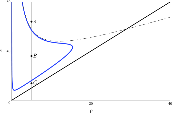
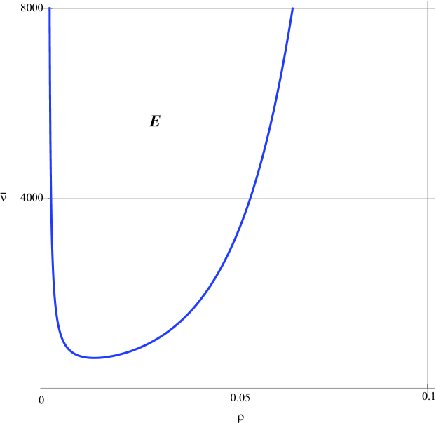
Figure 1: Bifurcation picture for $D_{max}=12$, $\kappa=1$, $T=1$, $\bar{T}=T/2$. The solid black line is $\bar{\nu}={\kappa\rho T}/{\bar{T}}$ (see (10)), the dashed line is $\bar{\nu}=\kappa(\rho+D_{max})^{2}/\rho$ and it is related to (7). Optimal patterns for $A$, $B$ and $C$ are shown on Fig. 3

Figure 2: The region $E$ with optimal constant control $u=1$. Below this region, this diagram is connected with Fig. 1

The only potential optimal control in that family is therefore $u(t)=1$ for all times. Using the expressions computed previously, this control can be a candidate optimal control law only if $y_{0}=y_{0min}$ as we have seen earlier and the complete dynamics should satisfy:

$$\bar{\lambda}\bar{y}\left(\frac{\bar{\mu}}{1+\bar{y}}-r-1\right)+\bar{y}=\lambda_{0}y_{0}\left(\frac{\bar{\mu}}{1+y_{0}}-r\right)$$ (26)

$$\bar{y}=\displaystyle y_{0}e^{(r+1)(T-\bar{T})}$$ (27)

$$\lambda_{0}=\displaystyle\bar{\lambda}e^{(r+1)(T-\bar{T})}-\displaystyle\frac{e^{(r+1)(T-\bar{T})}-1}{r+1}$$ (28)

with $\lambda_{0}<1$ and $\bar{\lambda}<1$.

4 Bifurcation analysis

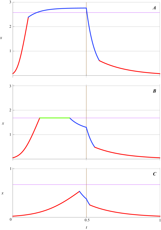
Figure 3: Different optimal patterns: (A) $\bar{\nu}=14$, (B) $\bar{\nu}=36$, (C) $\bar{\nu}=64$; $\rho=5$, $D_{max}=12$, $\kappa=1$, $T=1$, $\bar{T}=T/2$. Red: $u=0$, Blue: $u=1$, Green: intermediate control $u\in[0,1]$. Magenta line indicates the level $x=\kappa y_{\sigma}$ (see (8))

In this section, we will consider fixed values of all parameters except of $\bar{\nu}$ and $\rho$. We build a bifurcation diagram for these two parameters by identifying in which region no solution is possible (where (10) is not satisfied, it is below the solid black line on Fig. 1), and where the optimal solution is bang-singular-bang (Fig. 1, inside the blue curve), bang-bang (Fig. 1, outside the blue curve and above the solid black line), and constant at value $1$ (see Fig. 2). But the last case is only realized for extremely large values of $\bar{\nu}$. We see that the region where singular control can exist is smaller than what is defined by condition (21). This is due to the fact that, though the singular control is possible, there is not enough time for the control to reach that level (see Fig. 3(C)). For larger values of $\bar{\nu}$, no singular control is possible and the optimal solution in the light region goes toward the equilibrium corresponding to $u=1$ (see Fig. 3(A)). In that case, as well as in the bang-singular-bang case, the solutions go to the optimal solution of the constant light problem (Fig. 3(B)).

5 Conclusions

We have shown that, because of the day-night constraint, the productivity rate cannot be as high as it could have been without it. However, when the maximal growth rate is sufficiently larger than the respiration rate, we manage to have a temporary phase where the productivity rate is at or near this level. The maximal harvesting at the end of the light phase and at the beginning of the dark phase minimizes the biomass during the dark phase and, consequently, the net respiration. If the maximal growth rate is very large, the optimal solution consists in constantly applying maximal control because the biomass that is built-up in the light phase needs to be harvested even during the night.

References

- [1] O. Bernard, P. Masci and A. Sciandra, "A photobioreactor model in nitrogen limited conditions", in 6th Vienna International Conference on Mathematical Modelling MATHMOD 2009, Vienna, Austria, 2009.
- [2] Y. Chisti, Biodisel from microalgae. Biotechnology Advances, vol. 25, 2007, pp 294-306.
- [3] M. Droop, Vitamin B12 and marine ecology. IV. the kinetics of uptake growth and inhibition in Monochrysis lutheri. J. Mar. Biol. Assoc., vol. 48(3), 1968, pp 689-733.
- [4] J. Huismann et al., Principles of the light-limited chemostat: theory and ecological applications. Antonie van Leeuvenhoek, vol. 81, 2002, pp 117-133.
- [5] M. Huntley, D. Redalje, Co2 mitigation et renewable oil from photosynthetic microbes: A new appraisal. Mitigation et Adaptation Strategies for Global Change, vol. 12, 2007, pp 573-608.
- [6] E.G. Gilbert, Optimal Periodic Control: a General Theory of Necessary Conditions. SIAM J. Control and Optimization, vol. 15(5), 1977, pp 717-746.
- [7] A.A. Melikyan, Generalized Characteristics of First Order PDEs: Applications in Optimal Control and Differential Games. Birkhäuser, Boston; 1998.
- [8] P. Masci, O. Bernard, F. Grognard, Microalgal biomass productivity optimization based on a photobioreactor model, Computer Applications in Biotechnology, 2010.
- [9] J. Monod, Recherches sur la Croissance des Culteres Bactériennes. Herman, Paris; 1942.
- [10] L.S. Pontryagin, V.G. Boltyansky, R.V. Gamkrelidze, E.F. Mishchenko, Mathematical Theory of Optimal Processes. Wiley-Interscience, New York; 1962.
- [11] P. Spolaore, C. Joannis-Cassan, E. Duran, A. Isambert, Commercial applications of microalgae. Journal of Bioscience and Bioengineering, vol. 101(2), 2006, pp 87-96.