Topological recursion for the Poincaré polynomial of the combinatorial moduli space of curves

Abstract.

We show that the Poincaré polynomial associated with the orbifold cell decomposition of the moduli space of smooth algebraic curves with distinct marked points satisfies a topological recursion formula of the Eynard-Orantin type. The recursion uniquely determines the Poincaré polynomials from the initial data. Our key discovery is that the Poincaré polynomial is the Laplace transform of the number of Grothendieck’s dessins d’enfants.

1. Introduction

The Euler characteristic of the moduli space ${\mathcal{M}}_{g,n}$ of smooth algebraic curves of genus $g$ and $n$ distinct marked points has a closed formula

(1.1) $$\chi\left({\mathcal{M}}_{g,n}\right) =(-1)^{n-1}\frac{(2g-3+n)!}{(2g-2)!}\cdot\zeta(1-2g)$$

$$=(-1)^{n}\frac{(2g-3+n)!}{(2g)!}(2g-1)b_{2g}$$

due to Harer and Zagier [14], where $\zeta(s)$ is the Riemann zeta function and $b_{r}$ the Bernoulli number defined by

$$\frac{x}{e^{x}-1}=\sum_{r=0}\frac{b_{r}}{r!}\;x^{r}.$$

A relation of this formula to quantum field theory, in particular matrix models, was discovered by Penner [28], and a proof of (1.1) in terms of an asymptotic analysis of the Feynman diagram expansion of the Penner matrix model was established in [21].

A Feynman diagram for the Penner model is a double-edge graph of ’t Hooft [32], which we call a ribbon graph following Kontsevich [16]. The reason that ribbon graphs appear in the calculation of the Euler characteristic of the moduli space lies in the isomorphism of topological orbifolds

(1.2) $${{\mathcal{M}}}_{g,n}\times{\mathbb{R}}_{+}^{n}\cong RG_{g,n}$$

due to Harer [13], Mumford [25], and Strebel [31]. Here

(1.3) $$RG_{g,n}=\coprod_{\begin{subarray}{c}\Gamma{\text{ ribbon graph}}\\ {\text{of type }}(g,n)\end{subarray}}\frac{{\mathbb{R}}_{+}^{e(\Gamma)}}{{\text{\rm{Aut}}}(\Gamma)}$$

is the smooth orbifold [30] consisting of metric ribbon graphs of a given topological type $(g,n)$ with valence $3$ or more, $e(\Gamma)$ is the number of edges of the ribbon graph $\Gamma$, and ${\text{\rm{Aut}}}(\Gamma)$ is the group of ribbon graph automorphisms of $\Gamma$ that fix every face. The Penner model is the generating function of the Euler characteristic of $RG_{g,n}$. As an element of the formal power series in two variables $z$ and $M$, we have the equality

(1.4) $$\log\int_{{\mathcal{H}}_{M}}\exp\left(-\sum_{j=2}^{\infty}\frac{(\sqrt{z})^{j-2}}{j}\;{\text{\rm{trace}}}(X^{j})\right)dX\\ =\sum_{\begin{subarray}{c}g\geq 0,\;n>0\\ 2g-2+n>0\end{subarray}}(-1)^{n}\;\chi\left(RG_{g,n}\right)\frac{M^{n}}{n!}\;z^{2g-2+n},$$

where the parameter $M$ appears as the size of the Hermitian matrix $X$ in the left-hand side, ${\mathcal{H}}_{M}$ is the linear space of $M\times M$ Hermitian matrices, and $dX$ is a suitably normalized Lebesgue measure on ${\mathcal{H}}_{M}$. We refer to [21] for the precise meaning of the equality.

Although the matrix integral (1.4) gives an effective tool to calculate the Euler characteristic

$$\chi\left(RG_{g,n}\right)=\sum_{\begin{subarray}{c}\Gamma{\text{ ribbon graph}}\\ {\text{of type }}(g,n)\end{subarray}}\frac{(-1)^{e(\Gamma)}}{|{\text{\rm{Aut}}}(\Gamma)|},$$

it does not tell us anything about more refined information of the orbifold cell structure of $RG_{g,n}$. One can ask: Isn’t there any effective tool to find more numerical information about the orbifold $RG_{g,n}$?

The purpose of this paper is to answer this question. Our answer is again based on an idea from physics, this time utilizing the Eynard-Orantin topological recursion theory [8].

For a fixed $(g,n)$ in the stable range, i.e., $2g-2+n>0$, we choose $n$ variables $t_{1},t_{2},\dots,t_{n}$, and define the function

$$z(t_{i},t_{j})=\frac{(t_{i}+1)(t_{j}+1)}{2(t_{i}+t_{j})}.$$

An edge $\eta$ of a ribbon graph $\Gamma$ bounds two faces, say $i_{\eta}$ and $j_{\eta}$. These two faces may be actually the same. Now we define the Poincaré polynomial of $RG_{g,n}$ in the $z$-variables by

(1.5) $$F_{g,n}(t_{1},\dots,t_{n})=\sum_{\begin{subarray}{c}\Gamma{\text{ ribbon graph}}\\ {\text{of type }}(g,n)\end{subarray}}\frac{(-1)^{e(\Gamma)}}{|{\text{\rm{Aut}}}(\Gamma)|}\prod_{\begin{subarray}{c}\eta\text{ edge}\\ \text{of }\Gamma\end{subarray}}z\!\left(t_{i_{\eta}},t_{j_{\eta}}\right),$$

which is a polynomial in $z(t_{i},t_{j})$ but actually a symmetric rational function in $t_{1},\dots,t_{n}$. Our main theorem of this paper is a topological recursion formula that uniquely determines the Poincaré polynomials. To state the formula in a compact fashion, we use the following notation. Let $N=\{1,2,\dots,n\}$ be the index set labeling the marked points of a smooth algebraic curve. The faces of a ribbon graph of type $(g,n)$ are also labeled by the same set. For every subset $I\subset N$, we denote

$$t_{I}=\left(t_{i}\right)_{i\in I}.$$

Theorem 1.1.

The Poincaré polynomial $F_{g,n}(t_{N})$ with $(g,n)$ in the stable range

$$2g-2+n>0$$

is uniquely determined by the following topological recursion formula from the initial values $F_{0,3}(t_{1},t_{2},t_{3})$ and $F_{1,1}(t_{1})$.

(1.6) $$F_{g,n}(t_{N})\\ =-\frac{1}{16}\int_{-1}^{t_{1}}\Biggr{[}\sum_{j=2}^{n}\frac{t_{j}}{t^{2}-t_{j}^{2}}\Bigg{(}\frac{(t^{2}-1)^{3}}{t^{2}}\frac{\partial}{\partial t}F_{g,n-1}(t,t_{N\setminus\{1,j\}})-\frac{(t_{j}^{2}-1)^{3}}{t_{j}^{2}}\frac{\partial}{\partial t_{j}}F_{g,n-1}(t_{N\setminus\{1\}})\Bigg{)}\\ +\sum_{j=2}^{n}\frac{(t^{2}-1)^{2}}{t^{2}}\frac{\partial}{\partial t}F_{g,n-1}(t,t_{N\setminus\{1,j\}})\\ +\frac{1}{2}\;\frac{(t^{2}-1)^{3}}{t^{2}}\frac{\partial^{2}}{\partial u_{1}\partial u_{2}}\Bigg{(}F_{g-1,n+1}(u_{1},u_{2},t_{N\setminus\{1\}})\\ +\sum_{\begin{subarray}{c}g_{1}+g_{2}=g\\ I\sqcup J=N\setminus\{1\}\end{subarray}}^{\rm{stable}}F_{g_{1},|I|+1}(u_{1},t_{I})F_{g_{2},|J|+1}(u_{2},t_{J})\Bigg{)}\Bigg{|}_{u_{1}=u_{2}=t}\;\Biggr{]}\;dt.$$

Here the last sum is taken over all partitions $g_{1}+g_{2}=g$ and set partitions $I\sqcup J=N\setminus\{1\}$ subject to the stability conditions $2g_{1}-1+|I|>0$ and $2g_{2}-1+|J|>0$.

Remark 1.2.

1. It was shown in [5] that the symmetric differential $d_{1}\otimes\cdots\otimes d_{n}F_{g,n}(t_{N})$ satisfies an Eynard-Orantin type topological recursion. The relation between the Euler characteristic of ${\mathcal{M}}_{g,n}$ and the Eynard-Orantin theory was first pointed out in [27].

2. The word topological recursion refers to the inductive structure on the quantity $2g-2+n$, which is the absolute value of the Euler characteristic of an oriented $n$-punctured surface of genus $g$. Reduction of the quantity $2g-2+n$ by one has appeared in many recent works on moduli theory of curves, Gromov-Witten theory and related topics. This includes the operation of cutting off a pair of pants from a bordered surface as in [19, 20], the Hurwitz move or the cut-and-join equation of Hurwitz numbers [11, 15, 33], the edge removal operation on $RG_{g,n}$ of [5, 26], and many generalizations including [3, 4, 7, 17, 18, 23, 24, 35, 36].

By the definition of $F_{g,n}(t_{N})$ and the fact that $z(1,1)=1$, the Poincaré polynomial recovers the Euler characteristic of the moduli space ${\mathcal{M}}_{g,n}$ as the special value

$$F_{g,n}(1,1,\dots,1)=\chi\left(RG_{g,n}\right)=(-1)^{n}\chi\left({\mathcal{M}}_{g,n}\right).$$

The Poincaré polynomial becomes particularly simple when $n=1$. We have

(1.7) $$F_{g,1}(t)=\sum_{\begin{subarray}{c}\Gamma{\text{ ribbon graph}}\\ {\text{of type }}(g,1)\end{subarray}}\frac{(-1)^{e(\Gamma)}}{|{\text{\rm{Aut}}}(\Gamma)|}\;z^{e(\Gamma)},$$

where

(1.8) $$z=z(t,t)=\frac{(t+1)^{2}}{4t}.$$

An immediate generalization of the above formula is the diagonal value

(1.9) $$F_{g,n}(t,t,\dots,t)=\sum_{\begin{subarray}{c}\Gamma{\text{ ribbon graph}}\\ {\text{of type }}(g,n)\end{subarray}}\frac{(-1)^{e(\Gamma)}}{|{\text{\rm{Aut}}}(\Gamma)|}\;z^{e(\Gamma)}.$$

Because of this formula our terminology of calling $F_{g,n}(t_{N})$ the “Poincaré polynomial” is justified.

Although it is not obvious from the definition or even from Theorem 1.1, the symmetric rational function $F_{g,n}(t_{1},\dots,t_{n})$ is actually a Laurent polynomial. Therefore, it makes sense to extract the highest degree terms. If we naively extract the top degree term from $z(t_{i},t_{j})$, then we obtain

$$z^{\rm{top}}(t_{i},t_{j})=\frac{t_{i}t_{j}}{2(t_{i}+t_{j})}.$$

Since the number of edges of a ribbon graph is maximum for a trivalent graph, we obtain the following.

Theorem 1.3.

The Poincaré polynomial $F_{g,n}(t_{N})$ is a Laurent polynomial in $t_{1},t_{2},\dots,t_{n}$ of degree $3(2g-2+n)$ such that every monomial term contains only an odd power of each $t_{j}$. The leading homogeneous polynomial $F_{g,n}^{\rm{top}}(t_{N})$ of $F_{g,n}(t_{N})$ is given by

(1.10) $$F_{g,n}^{\rm{top}}(t_{N}) =\sum_{\begin{subarray}{c}\Gamma{\text{ trivalent ribbon}}\\ {\text{graph of type }}(g,n)\end{subarray}}\frac{(-1)^{e(\Gamma)}}{|{\text{\rm{Aut}}}(\Gamma)|}\prod_{\begin{subarray}{c}\eta\text{ edge}\\ \text{of }\Gamma\end{subarray}}\frac{t_{i_{\eta}}t_{j_{\eta}}}{2\left(t_{i_{\eta}}+t_{j_{\eta}}\right)}$$

$$=\frac{(-1)^{n}}{2^{5g-5+2n}}\sum_{\begin{subarray}{c}d_{1}+\cdots+d_{n}\\ =3g-3+n\end{subarray}}{\langle}\tau_{d_{1}}\cdots\tau_{d_{n}}{\rangle}_{g,n}\prod_{j=1}^{n}\frac{(2d_{j})!}{d_{j}!}\left(\frac{t_{j}}{2}\right)^{2d_{j}+1},$$

where

$${\langle}\tau_{d_{1}}\cdots\tau_{d_{n}}{\rangle}_{g,n}=\int_{{\overline{\mathcal{M}}}_{g,n}}c_{1}({\mathbb{L}}_{1})^{d_{1}}\cdots c_{1}({\mathbb{L}}_{n})^{d_{n}}$$

are the $\psi$-class intersection numbers of the tautological cotangent line bundles ${\mathbb{L}}_{1},\dots,{\mathbb{L}}_{n}$ on ${\overline{\mathcal{M}}}_{g,n}$. The above formula is identical to the boxed formula of Kontsevich [16, page 10]. The topological recursion (1.6) restricts to the leading terms $F_{g,n}^{\rm{top}}(t_{N})$ and recovers the Virasoro constraint condition, or the DVV-formula, of the $\psi$-class intersection numbers due to Dijkgraaf-Verlinde-Verlinde [6] and Witten [34].

It requires the deep theory of Mirzakhani [19, 20] to relate the leading terms $F_{g,n}^{\rm{top}}(t_{N})$ and the intersection numbers because of the difference between ${\mathcal{M}}_{g,n}$ and ${\overline{\mathcal{M}}}_{g,n}$. The contribution of Theorem 1.3 is to identify the origin of the Virasoro constraint condition as the edge-removal operation of ribbon graphs of [5, 26], and to clarify the relation between the combinatorics of counting problems and the geometry of intersection numbers. For the moduli space of vector bundles on curves, Harder and Narasimhan used Deligne’s solution of the Weil conjecture to obtain the Poincaré polynomial. Although what we are dealing with in this article is much simpler than the situation of [12], we find that again a counting problem plays a key role in calculating the Poincaré polynomial. Here the critical differences are that we use lattice point counting rather than moduli theory over the finite field ${\mathbb{F}}_{q}$, and that through (1.10) the counting problem also leads to the intersection numbers of the compactified moduli space ${\overline{\mathcal{M}}}_{g,n}$.

We note that the polynomial situation of Theorem 1.3 is similar to the case of simple Hurwitz numbers studied in [7, 24]. Indeed, the result of [24] is that the Laplace transform of simple Hurwitz numbers as a function of a partition is a polynomial that satisfies a topological recursion. This recursion proves the DVV formula of [6, 16, 34] when restricted to the leading terms, and also proves the $\lambda_{g}$-conjecture (the theorem of [9, 10]) when restricted to the lowest degree homogeneous terms. In a surprising similarity, we show that the Laurent polynomial $F_{g,n}(t_{1},\dots,t_{n})$ is the Laplace transform of the number of Grothendieck’s dessins d’enfants [1, 22, 29].

One can ask: Why does the Laplace transform appear in this context? A short answer is that the Laplace transform here is in fact the mirror map that transforms the A-model side of topological string theory to the B-model side. We do not investigate this idea any further in this paper, and refer to the introduction of [5, 7, 24] for more discussion.

This paper is organized as follows. We review the necessary information on the ribbon graph complex in Section 2. In Section 3, we recall the topological recursion for the number of lattice points of $RG_{g,n}$ that was established in [5]. We then show in Section 4 that the Laplace transform of this number is exactly the Poincaré polynomial of (1.5). A differential equation for the Poincaré polynomials is derived in Section 5. The initial values of the recursion formula are calculated in Section 6. In the final section we prove Theorem 1.1 and Theorem 1.3.

2. The combinatorial model of the moduli space

We begin by listing basic facts about ribbon graphs and the combinatorial model for the moduli space ${\mathcal{M}}_{g,n}$ due to Harer [13], Mumford [25] and Strebel [31], following [22]. Ribbon graphs are often referred to as Grothendieck’s dessins d’enphants. The standard literature on this subject is [29], which contains Grothendieck’s esquisse. We do not consider any number theoretic aspects of the dessins in this paper.

A ribbon graph of topological type $(g,n)$ is the $1$-skeleton of a cell-decomposition of a closed oriented topological surface $\Sigma$ of genus $g$ that decomposes the surface into a disjoint union of $v$ $0$-cells, $e$ $1$-cells, and $n$ $2$-cells. The Euler characteristic of the surface is given by $2-2g=v-e+n$. The $1$-skeleton of a cell-decomposition is a graph $\Gamma$ drawn on $\Sigma$, which consists of $v$ vertices and $e$ edges. An edge can form a loop. We denote by $\Sigma_{\Gamma}$ the cell-decomposed surface with $\Gamma$ its $1$-skeleton. Alternatively, a ribbon graph can be defined as a graph with a cyclic order given to the incident half-edges at each vertex. By abuse of terminology, we call the boundary of a $2$-cell of $\Sigma_{\Gamma}$ a boundary of $\Gamma$, and the $2$-cell itself as a face of $\Gamma$.

A metric ribbon graph is a ribbon graph with a positive real number (the length) assigned to each edge. For a given ribbon graph $\Gamma$ with $e=e(\Gamma)$ edges, the space of metric ribbon graphs is ${\mathbb{R}}_{+}^{e(\Gamma)}/{\text{\rm{Aut}}}(\Gamma)$, where the automorphism group acts by permutations of edges (see [22, Section 1]). We restrict ourselves to the case that ${\text{\rm{Aut}}}(\Gamma)$ fixes each $2$-cell of the cell-decomposition. We also require that every vertex of a ribbon graph has degree (i.e., valence) $3$ or more. Using the canonical holomorphic coordinate systems on a topological surface of [22, Section 4] and the Strebel differentials [31], we have an isomorphism of topological orbifolds [13, 25]

(2.1) $${{\mathcal{M}}}_{g,n}\times{\mathbb{R}}_{+}^{n}\cong RG_{g,n}.$$

Here

$$RG_{g,n}=\coprod_{\begin{subarray}{c}\Gamma{\text{ ribbon graph}}\\ {\text{of type }}(g,n)\end{subarray}}\frac{{\mathbb{R}}_{+}^{e(\Gamma)}}{{\text{\rm{Aut}}}(\Gamma)}$$

is the orbifold consisting of metric ribbon graphs of a given topological type $(g,n)$. The gluing of orbi-cells is done by making the length of a non-loop edge tend to $0$. The space $RG_{g,n}$ is a smooth orbifold (see [22, Section 3] and [30]). We denote by $\pi:RG_{g,n}\longrightarrow{\mathbb{R}}_{+}^{n}$ the natural projection via (2.1), which is the assignment of the collection of perimeter length of each boundary to a given metric ribbon graph.

Take a ribbon graph $\Gamma$. Since ${\text{\rm{Aut}}}(\Gamma)$ fixes every boundary component of $\Gamma$, they are labeled by $N=\{1,2\dots,n\}$. For the moment let us give a label to each edge of $\Gamma$ by an index set $E=\{1,2,\dots,e\}$. The edge-face incidence matrix is defined by

(2.2) $$A_{\Gamma} =\big{[}a_{i\eta}\big{]}_{i\in N,\;\eta\in E};$$

$$a_{i\eta} =\text{ the number of times edge $\eta$ appears in face $i$}.$$

Thus $a_{i\eta}=0,1,$ or $2$, and the sum of the entries in each column is always $2$. The $\Gamma$ contribution of the space $\pi^{-1}(p_{1},\dots,p_{n})=RG_{g,n}({\mathbf{p}})$ of metric ribbon graphs with a prescribed perimeter $\mathbf{p}=(p_{1},\dots,p_{n})$ is the orbifold polytope

$$P_{\Gamma}(\mathbf{p})/{\text{\rm{Aut}}}(\Gamma),\qquad P_{\Gamma}(\mathbf{p})=\{\mathbf{x}\in{\mathbb{R}}_{+}^{e}\;|\;A_{\Gamma}\mathbf{x}=\mathbf{p}\},$$

where $\mathbf{x}=(\ell_{1},\dots,\ell_{e})$ is the collection of edge lengths of the metric ribbon graph $\Gamma$. We have

(2.3) $$\sum_{i\in N}p_{i}=\sum_{i\in N}\sum_{\eta\in E}a_{i\eta}\ell_{\eta}=2\sum_{\eta\in E}\ell_{\eta}.$$

3. Topological recursion for the number of integral ribbon graphs

In this section we recall the topological recursion for the number of metric ribbon graphs $RG_{g,n}^{{\mathbb{Z}}_{+}}$ whose edges have integer lengths, following [5]. We call such a ribbon graph an integral ribbon graph. We can interpret an integral ribbon graph as Grothendieck’s dessin d’enfant by considering an edge of integer length as a chain of edges of length one connected by bivalent vertices, and reinterpreting the notion of ${\text{\rm{Aut}}}(\Gamma)$ suitably. Since we do not go into the number theoretic aspects of dessins, we stick to the more geometric notion of integral ribbon graphs.

Definition 3.1.

The weighted number $\big{|}RG_{g,n}^{{\mathbb{Z}}_{+}}({\mathbf{p}})\big{|}$ of integral ribbon graphs with prescribed perimeter lengths ${\mathbf{p}}\in{\mathbb{Z}}_{+}^{n}$ is defined by

(3.1) $$N_{g,n}({\mathbf{p}})=\big{|}RG_{g,n}^{{\mathbb{Z}}_{+}}({\mathbf{p}})\big{|}=\sum_{\begin{subarray}{c}\Gamma{\text{ ribbon graph}}\\ {\text{of type }}(g,n)\end{subarray}}\frac{\big{|}\{{\mathbf{x}}\in{\mathbb{Z}}_{+}^{e(\Gamma)}\;|\;A_{\Gamma}{\mathbf{x}}={\mathbf{p}}\}\big{|}}{|{\text{\rm{Aut}}}(\Gamma)|}.$$

Since the finite set $\{{\mathbf{x}}\in{\mathbb{Z}}_{+}^{e(\Gamma)}\;|\;A_{\Gamma}{\mathbf{x}}={\mathbf{p}}\}$ is a collection of lattice points in the polytope $P_{\Gamma}({\mathbf{p}})$ with respect to the canonical integral structure ${\mathbb{Z}}\subset{\mathbb{R}}$ of the real numbers, $N_{g,n}({\mathbf{p}})$ can be thought of counting the number of lattice points in $RG_{g,n}({\mathbf{p}})$ with a weight factor $1/|{\text{\rm{Aut}}}(\Gamma)|$ for each ribbon graph. The function $N_{g,n}({\mathbf{p}})$ is a symmetric function in ${\mathbf{p}}=(p_{1},\dots,p_{n})$ because the summation runs over all ribbon graphs of topological type $(g,n)$.

Remark 3.2.

Since the integral vector ${\mathbf{x}}$ is restricted to take strictly positive values, we would have $N_{g,n}({\mathbf{p}})=0$ if we were to substitute ${\mathbf{p}}=0$. This normalization is natural from the point of view of lattice point counting and Grothendieck’s dessins d’enphants. However, we do not make such a substitution in this paper because we consider ${\mathbf{p}}$ as a strictly positive integer vector. This situation is similar to Hurwitz theory [7, 24], where a partition $\mu$ is a strictly positive integer vector that plays the role of our ${\mathbf{p}}$. We note that a different assignment of values was suggested in [26, 27].

For brevity of notation, we denote by $p_{I}=(p_{i})_{i\in I}$ for a subset $I\in N=\{1,2\dots,n\}$. The cardinality of $I$ is denoted by $|I|$. The following topological recursion formula was proved in [5] using the idea of ciliation of a ribbon graph.

Theorem 3.3 ([5]).

The number of integral ribbon graphs with prescribed boundary lengthes satisfies the topological recursion formula

(3.2) $$p_{1}N_{g,n}(p_{N})={\frac{1}{2}}\sum_{j=2}^{n}\Bigg{[}\sum_{q=0}^{p_{1}+p_{j}}q(p_{1}+p_{j}-q)N_{g,n-1}(q,p_{N\setminus\{1,j\}})\\ +H(p_{1}-p_{j})\sum_{q=0}^{p_{1}-p_{j}}q(p_{1}-p_{j}-q)N_{g,n-1}(q,p_{N\setminus\{1,j\}})\\ -H(p_{j}-p_{1})\sum_{q=0}^{p_{j}-p_{1}}q(p_{j}-p_{1}-q)N_{g,n-1}(q,p_{N\setminus\{1,j\}})\Bigg{]}\\ +{\frac{1}{2}}\sum_{0\leq q_{1}+q_{2}\leq p_{1}}q_{1}q_{2}(p_{1}-q_{1}-q_{2})\Bigg{[}N_{g-1,n+1}(q_{1},q_{2},p_{N\setminus\{1\}})\\ +\sum_{\begin{subarray}{c}g_{1}+g_{2}=g\\ I\sqcup J=N\setminus\{1\}\end{subarray}}^{\rm{stable}}N_{g_{1},|I|+1}(q_{1},p_{I})N_{g_{2},|J|+1}(q_{2},p_{J})\Bigg{]}.$$

Here

$$H(x)=\begin{cases}1\qquad x>0\\ 0\qquad x\leq 0\end{cases}$$

is the Heaviside function, and the last sum is taken for all partitions $g=g_{1}+g_{2}$ and $I\sqcup J=N\setminus\{1\}$ subject to the stability conditions $2g_{1}-1+{I}>0$ and $2g_{2}-1+|J|>0$.

4. The Laplace transform of the number of integral ribbon graphs

Let us consider the Laplace transform

(4.1) $$L_{g,n}(w_{1},\dots,w_{n})\overset{\rm{def}}{=}\sum_{{\mathbf{p}}\in{\mathbb{Z}}_{+}^{n}}N_{g,n}({\mathbf{p}})e^{-{\langle}{\mathbf{p}},w{\rangle}}$$

of the number of integral ribbon graphs $N_{g,n}({\mathbf{p}})$, where ${\langle}{\mathbf{p}},w{\rangle}=p_{1}w_{1}+\cdots+p_{n}w_{n}$, and the summation is taken over all integer vectors ${\mathbf{p}}\in{\mathbb{Z}}_{+}^{n}$ of strictly positive entries. In this section we prove that after the coordinate change of [5] from the $w$-coordinates to the $t$-coordinates defined by

(4.2) $$e^{-w_{j}}=\frac{t_{j}+1}{t_{j}-1},\qquad j=1,2,\dots,n,$$

the Laplace transform $L_{g,n}(w_{N})$ becomes the Poincaré polynomial

(4.3) $$F_{g,n}(t_{1},\dots,t_{n})=L_{g,n}\big{(}w_{1}(t),\dots,w_{n}(t)\big{)}.$$

The Laplace transform $L_{g,n}(w_{N})$ can be evaluated using the definition of the number of integral ribbon graphs (3.1). Let $a_{\eta}$ be the $\eta$-th column of the incidence matrix $A_{\Gamma}$ so that

(4.4) $$A_{\Gamma}=\big{[}a_{1}\big{|}a_{2}\big{|}\cdots\big{|}a_{e(\Gamma)}\big{]}.$$

Then

(4.5) $$L_{g,n}(w_{N})=\sum_{{\mathbf{p}}\in{\mathbb{Z}}_{+}^{n}}N_{g,n}({\mathbf{p}})e^{-{\langle}{\mathbf{p}},w{\rangle}}\\ =\sum_{\begin{subarray}{c}\Gamma{\text{ ribbon graph}}\\ {\text{of type }}(g,n)\end{subarray}}\sum_{{\mathbf{p}}\in{\mathbb{Z}}_{+}^{n}}\frac{1}{|{\text{\rm{Aut}}}(\Gamma)|}\big{|}\{{\mathbf{x}}\in{\mathbb{Z}}_{+}^{e(\Gamma)}\;|\;A_{\Gamma}{\mathbf{x}}={\mathbf{p}}\}\big{|}e^{-{\langle}{\mathbf{p}},w{\rangle}}\\ =\sum_{\begin{subarray}{c}\Gamma{\text{ ribbon graph}}\\ {\text{of type }}(g,n)\end{subarray}}\frac{1}{|{\text{\rm{Aut}}}(\Gamma)|}\sum_{{\mathbf{x}}\in{\mathbb{Z}}_{+}^{e(\Gamma)}}e^{-{\langle}A_{\Gamma}{\mathbf{x}},w{\rangle}}\\ =\sum_{\begin{subarray}{c}\Gamma{\text{ ribbon graph}}\\ {\text{of type }}(g,n)\end{subarray}}\frac{1}{|{\text{\rm{Aut}}}(\Gamma)|}\prod_{\begin{subarray}{c}\eta\text{ edge}\\ \text{of }\Gamma\end{subarray}}\sum_{\ell_{\eta}=1}^{\infty}e^{-{\langle}a_{\eta},w{\rangle}\ell_{\eta}}\\ =\sum_{\begin{subarray}{c}\Gamma{\text{ ribbon graph}}\\ {\text{of type }}(g,n)\end{subarray}}\frac{1}{|{\text{\rm{Aut}}}(\Gamma)|}\prod_{\begin{subarray}{c}\eta\text{ edge}\\ \text{of }\Gamma\end{subarray}}\frac{e^{-{\langle}a_{\eta},w{\rangle}}}{1-e^{-{\langle}a_{\eta},w{\rangle}}}.$$

Every edge $\eta$ bounds two faces, which we call face $i_{\eta}^{+}$ and face $i_{\eta}^{-}$. When $a_{i\eta}=2$, these faces are the same. We then calculate

(4.6) $$\frac{e^{-{\langle}a_{\eta},w{\rangle}}}{1-e^{-{\langle}a_{\eta},w{\rangle}}}=-z\!\left(t_{i_{\eta}^{+}},t_{i_{\eta}^{-}}\right),$$

where

(4.7) $$z(t_{i},t_{j})\overset{\rm{def}}{=}\frac{(t_{i}+1)(t_{j}+1)}{2(t_{i}+t_{j})}.$$

This follows from (4.2) and

$$\frac{e^{-(w_{i}+w_{j})}}{1-e^{-(w_{i}+w_{j})}} =\frac{\frac{(t_{i}+1)(t_{j}+1)}{(t_{i}-1)(t_{j}-1)}}{1-\frac{(t_{i}+1)(t_{j}+1)}{(t_{i}-1)(t_{j}-1)}}=-\frac{(t_{i}+1)(t_{j}+1)}{2(t_{i}+t_{j})}=-z(t_{i},t_{j}),$$

$$\frac{e^{-2w_{i}}}{1-e^{-2w_{i}}} =-\frac{(t_{i}+1)^{2}}{4t_{i}}=-z(t_{i},t_{i}).$$

Note that since $z(t_{i},t_{j})$ is a symmetric function, which face is named $i_{\eta}^{+}$ or $i_{\eta}^{-}$ does not matter. From (4.5) and (4.6), we have established

Theorem 4.1.

The Laplace transform $L_{g,n}(w_{N})$ in terms of the $t$-coordinates (4.2) is the Poincaré polynomial

(4.8) $$F_{g,n}(t_{N})=\sum_{\begin{subarray}{c}\Gamma{\text{ ribbon graph}}\\ {\text{of type }}(g,n)\end{subarray}}\frac{(-1)^{e(\Gamma)}}{|{\text{\rm{Aut}}}(\Gamma)|}\prod_{\begin{subarray}{c}\eta\text{ edge}\\ \text{of }\Gamma\end{subarray}}z\!\left(t_{i_{\eta}^{+}},t_{i_{\eta}^{-}}\right).$$

Corollary 4.2.

The evaluation of $F_{g,n}(t_{N})$ at $t_{1}=\cdots=t_{n}=1$ gives the Euler characteristic of $RG_{g,n}$

(4.9) $$F_{g,n}(1,1\dots,1)=\chi\left(RG_{g,n}\right)=(-1)^{n}\chi\left({\mathcal{M}}_{g,n}\right).$$

Furthermore, if we evaluate at $t_{j}=-1$ for any $j$, then we have

(4.10) $$F_{g,n}(t_{1},t_{2}\dots,t_{n})\big{|}_{t_{j}=-1}=0$$

as a function in the rest of the variables $t_{N\setminus\{j\}}$.

Proof.

The Euler characteristic calculation immediately follows from $z(1,1)=1$.

Consider a ribbon graph $\Gamma$ of type $(g,n)$. Its $j$-th face has at least one edge on its boundary. Therefore,

$$\prod_{\eta\text{ edge of }\Gamma}z\!\left(t_{i_{\eta}^{+}},t_{i_{\eta}^{-}}\right)$$

has a factor $(t_{j}+1)$ by (4.7). It holds for every ribbon graph $\Gamma$ in the summation of (4.8). Therefore, (4.10) follows. ∎

5. Topological recursion for the Poincaré polynomials

In this section we prove that the Poincaré polynomials satisfy a differential equation.

Theorem 5.1.

The Poincaré polynomial $F_{g,n}(t_{N})$ satisfies the following differential recursion equation.

(5.1) $$\frac{\partial}{\partial t_{1}}F_{g,n}(t_{N})\\ =-\frac{1}{16}\sum_{j=2}^{n}\left[\frac{t_{j}}{t_{1}^{2}-t_{j}^{2}}\left(\frac{(t_{1}^{2}-1)^{3}}{t_{1}^{2}}\frac{\partial}{\partial t_{1}}F_{g,n-1}(t_{N\setminus\{j\}})-\frac{(t_{j}^{2}-1)^{3}}{t_{j}^{2}}\frac{\partial}{\partial t_{j}}F_{g,n-1}(t_{N\setminus\{1\}})\right)\right]\\ -\frac{1}{16}\sum_{j=2}^{n}\frac{(t_{1}^{2}-1)^{2}}{t_{1}^{2}}\frac{\partial}{\partial t_{1}}F_{g,n-1}(t_{N\setminus\{j\}})\\ -\frac{1}{32}\;\frac{(t_{1}^{2}-1)^{3}}{t_{1}^{2}}\frac{\partial^{2}}{\partial u_{1}\partial u_{2}}\Bigg{[}F_{g-1,n+1}(u_{1},u_{2},t_{N\setminus\{1\}})\\ +\sum_{\begin{subarray}{c}g_{1}+g_{2}=g\\ I\sqcup J=N\setminus\{1\}\end{subarray}}^{\rm{stable}}F_{g_{1},|I|+1}(u_{1},t_{I})F_{g_{2},|J|+1}(u_{2},t_{J})\Bigg{]}\Bigg{|}_{u_{1}=u_{2}=t_{1}}.$$

Proof.

We first calculate the Laplace transform of (3.2) and establish a differential equation for $L_{g,n}(w_{N})$. We then change the variables from $w_{N}$ to $t_{N}$ using (4.2). The operation we need to do is to multiply both sides of (3.2) by $e^{-{\langle}{\mathbf{p}},w{\rangle}}$ and take the sum with respect to all integers $p_{1}\geq 0$ and $p_{N\setminus\{1\}}\in{\mathbb{Z}}_{+}^{n-1}$. Since the left-hand side of (3.2) is $p_{1}N_{g,n}(p_{N})$, we can allow $p_{1}=0$ in the summation.

The result of this operation to the left-hand side of (3.2) is $-\frac{\partial}{\partial w_{1}}L_{g,n}(w_{N})$. The operation applied to the first line of the right-hand side gives

(5.2) $$\sum_{j=2}^{n}\sum_{p_{1}=0}^{\infty}\sum_{p_{N\setminus\{1\}}\in{\mathbb{Z}}_{+}^{n-1}}\sum_{q=0}^{p_{1}+p_{j}}q\;\frac{p_{1}+p_{j}-q}{2}\;N_{g,n-1}(q,p_{N\setminus\{1,j\}})e^{-{\langle}{\mathbf{p}},w{\rangle}}\\ =\sum_{j=2}^{n}\sum_{q=0}^{\infty}\sum_{p_{N\setminus\{1,j\}}\in{\mathbb{Z}}_{+}^{n-2}}q\;N_{g,n-1}(q,p_{N\setminus\{1,j\}})e^{-{\langle}p_{N\setminus\{1,j\}},w_{N\setminus\{1,j\}}{\rangle}}e^{-qw_{1}}\\ \times\sum_{\ell=0}^{\infty}\ell e^{-2\ell w_{1}}\sum_{p_{j}=1}^{q+2\ell}e^{p_{j}(w_{1}-w_{j})},$$

where we set $p_{1}+p_{j}-q=2\ell$. Note that $N_{g,n}(p_{N})=0$ unless $p_{1}+\cdots+p_{n}$ is even, because of (2.3). Therefore, in the Laplace transform we are summing over all $p_{N}\in{\mathbb{Z}}_{+}^{n}$ such that $p_{1}+\cdots+p_{n}\equiv 0\mod 2$. Since $N_{g,n-1}(q,p_{N\setminus\{1,j\}})=0$ unless $q+p_{2}+\cdots+\widehat{p_{j}}+\cdots+p_{n}\equiv 0\mod 2$, only those $p_{1},p_{j}$ and $q$ satisfying $p_{1}+p_{j}-q\equiv 0\mod 2$ contribute in the summation. Thus we can replace $p_{1}+p_{j}-q$ by $2\ell$. The $p_{j}$-summation of (5.2) gives

$$\sum_{p_{j}=1}^{q+2\ell}e^{-qw_{1}}\ell e^{-2\ell w_{1}}e^{p_{j}(w_{1}-w_{j})}=\ell e^{-(q+2\ell)w_{1}}\frac{e^{w_{1}-w_{j}}-e^{(1+q+2\ell)(w_{1}-w_{j})}}{1-e^{w_{1}-w_{j}}}\\ =\frac{e^{w_{1}-w_{j}}}{1-e^{w_{1}-w_{j}}}\left(e^{-qw_{1}}\ell e^{-2\ell w_{1}}-e^{-qw_{j}}\ell e^{-2\ell w_{j}}\right).$$

Since the $\ell$-summation and the $q$-summation are separated now, (5.2) becomes

$$\sum_{j=2}^{n}\frac{e^{w_{1}-w_{j}}}{1-e^{w_{1}-w_{j}}}\Bigg{[}\frac{1}{(e^{w_{1}}-e^{-w_{1}})^{2}}\left(-\frac{\partial}{\partial w_{1}}\right)L_{g,n-1}(w_{N\setminus\{j\}})\\ -\frac{1}{(e^{w_{j}}-e^{-w_{j}})^{2}}\left(-\frac{\partial}{\partial w_{j}}\right)L_{g,n-1}(w_{N\setminus\{1\}})\Bigg{]}.$$

The second line of (3.2) gives

$$\sum_{j=2}^{n}\sum_{p_{1}=0}^{\infty}\sum_{p_{N\setminus\{1\}}\in{\mathbb{Z}}_{+}^{n-1}}H(p_{1}-p_{j})\sum_{q=0}^{p_{1}-p_{j}}q\;\frac{p_{1}-p_{j}-q}{2}N_{g,n-1}(q,p_{N\setminus\{1,j\}})e^{-{\langle}{\mathbf{p}},w{\rangle}}\\ =\sum_{j=2}^{n}\sum_{\ell=0}^{\infty}\ell e^{-2\ell w_{1}}\sum_{p_{j}=1}^{\infty}e^{-p_{j}(w_{1}+w_{j})}\\ \times\sum_{q=0}^{\infty}e^{-qw_{1}}\sum_{p_{N\setminus\{1,j\}}\in{\mathbb{Z}}_{+}^{n-2}}q\;N_{g,n-1}(q,p_{N\setminus\{1,j\}})e^{-{\langle}p_{N\setminus\{1,j\}},w_{N\setminus\{1,j\}}{\rangle}}\\ =\sum_{j=2}^{n}\frac{e^{-(w_{1}+w_{j})}}{1-e^{-(w_{1}+w_{j})}}\;\frac{1}{(e^{w_{1}}-e^{-w_{1}})^{2}}\left(-\frac{\partial}{\partial w_{1}}\right)L_{g,n-1}(w_{N\setminus\{j\}})\\ =\sum_{j=2}^{n}\left(\frac{1}{1-e^{-(w_{1}+w_{j})}}-1\right)\frac{1}{(e^{w_{1}}-e^{-w_{1}})^{2}}\left(-\frac{\partial}{\partial w_{1}}\right)L_{g,n-1}(w_{N\setminus\{j\}}),$$

where we set $p_{1}-p_{j}-q=2\ell$. Similarly, after putting $p_{j}-p_{1}-q=2\ell$, the third line of (3.2) yields

$$-\sum_{j=2}^{n}\sum_{p_{1}=0}^{\infty}\sum_{p_{N\setminus\{1\}}\in{\mathbb{Z}}_{+}^{n-1}}H(p_{j}-p_{1})\sum_{q=0}^{p_{j}-p_{1}}q\;\frac{p_{j}-p_{1}-q}{2}N_{g,n-1}(q,p_{N\setminus\{1,j\}})e^{-{\langle}{\mathbf{p}},w{\rangle}}\\ =-\sum_{j=2}^{n}\sum_{p_{1}=0}^{\infty}e^{-p_{1}(w_{1}+w_{j})}\sum_{\ell=0}^{\infty}\ell e^{-2\ell w_{j}}\\ \times\sum_{q=0}^{\infty}e^{-qw_{j}}\sum_{p_{N\setminus\{1,j\}}\in{\mathbb{Z}}_{+}^{n-2}}q\;N_{g,n-1}(q,p_{N\setminus\{1,j\}})e^{-{\langle}p_{N\setminus\{1,j\}},w_{N\setminus\{1,j\}}{\rangle}}\\ =-\sum_{j=2}^{n}\frac{1}{1-e^{-(w_{1}+w_{j})}}\;\frac{1}{(e^{w_{j}}-e^{-w_{j}})^{2}}\left(-\frac{\partial}{\partial w_{j}}\right)L_{g,n-1}(w_{N\setminus\{1\}}).$$

Summing all contributions, we obtain

$$\sum_{j=2}^{n}\left(\frac{e^{w_{1}-w_{j}}}{1-e^{w_{1}-w_{j}}}+\frac{1}{1-e^{-(w_{1}+w_{j})}}\right)\Bigg{[}\frac{1}{(e^{w_{1}}-e^{-w_{1}})^{2}}\left(-\frac{\partial}{\partial w_{1}}\right)L_{g,n-1}(w_{N\setminus\{j\}})\\ -\frac{1}{(e^{w_{j}}-e^{-w_{j}})^{2}}\left(-\frac{\partial}{\partial w_{j}}\right)L_{g,n-1}(w_{N\setminus\{1\}})\Bigg{]}\\ -\frac{1}{(e^{w_{1}}-e^{-w_{1}})^{2}}\left(-\frac{\partial}{\partial w_{1}}\right)\sum_{j=2}^{n}L_{g,n-1}(w_{N\setminus\{j\}}).$$

To compute the result of our operation to the fourth and the fifth lines of (3.2), we note that for any function $f(q_{1},q_{2})$ we have

$${\frac{1}{2}}\sum_{p_{1}=0}^{\infty}\sum_{0\leq q_{1}+q_{2}\leq p_{1}}q_{1}q_{2}(p_{1}-q_{1}-q_{2})e^{-p_{1}w_{1}}f(q_{1},q_{2})\\ ={\frac{1}{2}}\sum_{q_{1}=0}^{\infty}\sum_{q_{2}=0}^{\infty}\sum_{\ell=0}^{\infty}2\ell e^{-2\ell w_{1}}e^{-(q_{1}+q_{2})w_{1}}q_{1}q_{2}f(q_{1},q_{2})\\ =\frac{1}{(e^{w_{1}}-e^{-w_{1}})^{2}}\left.\frac{\partial^{2}}{\partial u_{1}\partial u_{2}}\widehat{f}(u_{1},u_{2})\right|_{u_{1}=u_{2}=w_{1}},$$

where we set $p_{1}-q_{1}-q_{2}=2\ell$, and

$$\widehat{f}(u_{1},u_{2})=\sum_{q_{1}=1}^{\infty}\sum_{q_{2}=1}^{\infty}f(q_{1},q_{2})e^{-(q_{1}u_{1}+q_{2}u_{2})}.$$

The reason that $p_{1}-q_{1}-q_{2}$ is even comes from the fact that we are summing over $p_{N}\in{\mathbb{Z}}_{+}^{n}$ subject to $p_{1}+\cdots+p_{n}\equiv 0\mod 2$, while in the fourth line of (3.2) contributions vanish unless $q_{1}+q_{2}+p_{2}+\cdots+p_{n}\equiv 0\mod 2$. Therefore, we can restrict the summation over those $p_{1},q_{1}$ and $q_{2}$ subject to $p_{1}\equiv q_{1}+q_{2}\mod 2$. The same condition can be imposed on the summation for the fifth line of (3.2).

Adding all the above, we establish

(5.3) $$\frac{\partial}{\partial w_{1}}L_{g,n}(w_{N})\\ =\sum_{j=2}^{n}\left(\frac{e^{w_{1}-w_{j}}}{1-e^{w_{1}-w_{j}}}+\frac{1}{1-e^{-(w_{1}+w_{j})}}\right)\Bigg{[}\frac{1}{(e^{w_{1}}-e^{-w_{1}})^{2}}\;\frac{\partial}{\partial w_{1}}L_{g,n-1}(w_{N\setminus\{j\}})\\ -\frac{1}{(e^{w_{j}}-e^{-w_{j}})^{2}}\;\frac{\partial}{\partial w_{j}}L_{g,n-1}(w_{N\setminus\{1\}})\Bigg{]}\\ -\sum_{j=2}^{n}\frac{1}{(e^{w_{1}}-e^{-w_{1}})^{2}}\;\frac{\partial}{\partial w_{1}}L_{g,n-1}(w_{N\setminus\{j\}})\\ -\frac{1}{(e^{w_{1}}-e^{-w_{1}})^{2}}\;\frac{\partial^{2}}{\partial u_{1}\partial u_{2}}\Bigg{[}L_{g-1,n+1}(u_{1},u_{2},w_{N\setminus\{1\}})\\ +\sum_{\begin{subarray}{c}g_{1}+g_{2}=g\\ I\sqcup J=N\setminus\{1\}\end{subarray}}^{\rm{stable}}L_{g_{1},|I|+1}(u_{1},w_{I})L_{g_{2},|J|+1}(u_{2},w_{J})\Bigg{]}\Bigg{|}_{u_{1}=u_{2}=w_{1}}.$$

From (4.2) we find

$$\frac{\partial}{\partial w_{j}} =\frac{t_{j}^{2}-1}{2}\;\frac{\partial}{\partial t_{j}}$$

$$\frac{1}{(e^{w_{j}}-e^{-w_{j}})^{2}} =\frac{1}{16}\;\frac{(t_{j}^{2}-1)^{2}}{t_{j}^{2}}$$

$$\frac{e^{w_{1}-w_{j}}}{1-e^{w_{1}-w_{j}}}+\frac{1}{1-e^{-(w_{1}+w_{j})}} =-\frac{t_{j}(t_{1}^{2}-1)}{t_{1}^{2}-t_{j}^{2}}.$$

It is now a straightforward calculation to convert (5.3) to (5.1). ∎

6. Initial values

In this section we calculate the initial values $F_{0,3}(t_{1},t_{2},t_{3})$ and $F_{1,1}(t)$.

   

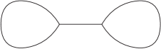
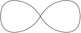
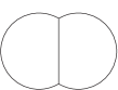
Figure 6.1. Three kinds of ribbon graphs of type $(0,3)$.

There are three kinds of ribbon graphs of type $(g,n)=(0,3)$ as listes in Figure 6.1. Each graph has no nontrivial automorphisms since every face is fixed. Therefore, we have

(6.1) $$F_{0,3}(t_{1},t_{2},t_{3})\\ =(-1)^{3}\bigg{(}z(t_{1},t_{1})z(t_{1},t_{2})z(t_{1},t_{3})+z(t_{2},t_{2})z(t_{2},t_{1})z(t_{2},t_{3})+z(t_{3},t_{3})z(t_{3},t_{1})z(t_{3},t_{2})\bigg{)}\\ +(-1)^{2}\bigg{(}z(t_{1},t_{2})z(t_{1},t_{3})+z(t_{2},t_{1})z(t_{2},t_{3})+z(t_{3},t_{1})z(t_{3},t_{2})\bigg{)}\\ +(-1)^{3}z(t_{1},t_{2})z(t_{1},t_{3})z(t_{2},t_{3})\\ =-\frac{1}{16}(t_{1}+1)(t_{2}+1)(t_{3}+1)\left(1+\frac{1}{t_{1}\;t_{2}\;t_{3}}\right).$$

The first line of the right-hand side of (6.1) corresponds to the dumbbell shape (the left graph of Figure 6.1), the second line to the infinity sign (the center graph of Figure 6.1), and the third line to the right graph of Figure 6.1.

                      

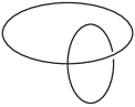
Figure 6.2. Two kinds of ribbon graphs of type $(1,1)$.

There are two graphs of type $(g,n)=(1,1)$, as shown in Figure 6.2. The graph on the left has automorphism group ${\mathbb{Z}}/6{\mathbb{Z}}$, and the graph on the right has automorphism group ${\mathbb{Z}}/4{\mathbb{Z}}$. Thus we have

(6.2) $$F_{1,1}(t)=\frac{(-1)^{3}}{6}z(t,t)^{3}+\frac{(-1)^{2}}{4}z(t,t)^{2}=-\frac{1}{384}\;\frac{(t+1)^{4}}{t^{2}}\left(t-4+\frac{1}{t}\right).$$

7. Consequences of the differential equation

Since (5.1) is a differential equation, we need to determine the initial condition with respect to the variable $t_{1}$ in order to uniquely solve it for $F_{g,n}(t_{N})$. In this section, we prove Theorem 1.1 by determining the initial value for the differential equation (5.1).

Theorem 7.1.

The Poincaré polynomial $F_{g,n}(t_{N})$ is uniquely determined by the differential equation (5.1) and the vanishing property (4.10).

Proof.

Suppose we have determined $F_{g,n}(t_{N})$ for all values of $(g,n)$ subject to

$$0<2g-2+n<m-1$$

for a given $m\geq 2$. Take any $(g,n)$ such that $2g-2+n=m$. Then (5.1) determines $\frac{\partial}{\partial t_{1}}F_{g,n}(t_{N})$. We denote by $r(t_{N})$ the right-hand side of (5.1), and define

(7.1) $$F_{g,n}(t_{N})=\int_{-1}^{t_{1}}r(t_{N})dt_{1}.$$

The lower bound is chosen so that (4.10) holds. Since $F_{g,n}(-1,t_{2},\dots,t_{n})=0$ as a function in $t_{N\setminus\{1\}}$, there is no room to add any function in $t_{N\setminus\{1\}}$ to the right-hand side of (7.1). We have thus uniquely determined $F_{g,n}(t_{N})$. This completes the proof. ∎

Since formula (7.1) is (1.6), we have thus proved Theorem 1.1.

The definition of the Poincaré polynomial (1.5) contains a factor like $\frac{1}{t_{i}+t_{j}}$. Surprisingly, $F_{g,n}(t_{N})$ is indeed a Laurent polynomial.

Theorem 7.2.

The Poincaré polynomial $F_{g,n}(t_{N})$ is a Laurent polynomial in $t_{1},t_{2},\dots,t_{n}$ of degree $3(2g-2+n)$. Moreover, every monomial appearing in $F_{g,n}(t_{N})$ contains only an odd power of each $t_{j}$.

Proof.

Here again suppose the statement is true for all values of $(g,n)$ subject to

$$0<2g-2+n<m-1$$

for a given $m\geq 2$. Take an arbitrary $(g,n)$ such that $2g-2+n=m$. Let $r(t_{N})$ denote the right-hand side of (5.1). There are two issues we need to address. The first one is division by $(t_{1}^{2}-t_{j}^{2})$ in the first line of $r(t_{N})$, since $\frac{1}{t_{1}^{2}-t_{j}^{2}}$ is not a Laurent polynomial. The second issue is the integration (7.1), which could produce logarithmic terms.

Lemma 7.3.

Consider a Laurent polynomial in one variable $f(x)$ that contains only odd powers of $x$. Then

(7.2) $$\frac{y}{x^{2}-y^{2}}\left(\frac{(x^{2}-1)^{3}}{x^{2}}\frac{\partial}{\partial x}\;f(x)-\frac{(y^{2}-1)^{3}}{y^{2}}\frac{\partial}{\partial y}\;f(y)\right)$$

is a Laurent polynomial in $x$ and $y$ such that each monomial contains only an even power of $x$ and an odd power of $y$.

If $h(x)$ is a Laurent polynomial in $x^{2}$, then $\frac{h(x)-h(y)}{x^{2}-y^{2}}$ is a Laurent polynomial in $x^{2}$ and $y^{2}$. Therefore,

$$\frac{1}{x^{2}-y^{2}}\left(\frac{(x^{2}-1)^{3}}{x^{2}}\frac{\partial}{\partial x}\;f(x)-\frac{(y^{2}-1)^{3}}{y^{2}}\frac{\partial}{\partial y}\;f(y)\right)$$

is a Laurent polynomial in $x^{2}$ and $y^{2}$. This proves the lemma.

Thus we know that $r(t_{N})$ is a Laurent polynomial in $t_{1},\dots,t_{n}$ such that each monomial contains an even power of $t_{1}$ and an odd powers of $t_{j}$ for every $j>1$. Therefore,

$$F_{g,n}(t_{N})=\int_{-1}^{t_{1}}r(t_{N})dt_{1}$$

is a Laurent polynomial in $t_{1},\dots,t_{n}$ such that every monomial term contains only an odd power of each $t_{j}$. This completes the proof of the theorem. ∎

Based on the work [2], it is noted in [5] that the symmetric homogeneous polynomial in $t_{1},\dots,t_{n}$ consisting of the leading terms of

$$2^{5g-5+2n}\;\frac{\partial^{n}}{\partial t_{1}\cdots\partial t_{n}}F_{g,n}(t_{N})$$

is the generating function of the $\psi$-class intersection numbers on the Deligne-Mumford stack ${\overline{\mathcal{M}}}_{g,n}$ considered in [6, 16, 34], and that the restriction of the recursion (5.1) to the leading terms, after taking the differentiation with respect to $t_{2},\dots,t_{n}$, is equivalent to the Virasoro constraint condition of the $\psi$-class intersection numbers. This proves Theorem 1.3.

Although we do not utilize the following fact in this paper, we note that the Laurent polynomial $F_{g,n}(t_{N})$ is invariant under the coordinate change $t_{j}\longmapsto\frac{1}{t_{j}}$. This is because

$$z(t_{i},t_{j})=z\!\left(\frac{1}{t_{i}},\frac{1}{t_{j}}\right).$$

Proposition 7.4.

The Poincaré polynomial is invariant under the transformation $t_{j}\longmapsto\frac{1}{t_{j}}$

$$F_{g,n}(t_{1},t_{2},\dots,t_{n})=F_{g,n}\!\left(\frac{1}{t_{1}},\frac{1}{t_{2}},\dots,\frac{1}{t_{n}}\right).$$

Appendix A Examples

We record a few examples of the Poincaré polynomials here.

(A.1) $$F_{0,4}(t_{1},t_{2},t_{3},t_{4})=\frac{1}{2^{8}}\;(t_{1}+1)(t_{2}+1)(t_{3}+1)(t_{4}+1)\\ \times\left[\sum_{j=1}^{4}t_{j}^{2}-\sum_{j=1}^{4}t_{j}-5-\sum_{i<j}\frac{1}{t_{i}t_{j}}+\frac{1}{t_{1}t_{2}t_{3}t_{4}}\left(-5-\sum_{j=1}^{4}\frac{1}{t_{j}}+\sum_{j=1}^{4}\frac{1}{t_{j}^{2}}\right)\right].$$

(A.2) $$F_{1,2}(t_{1},t_{2})=\frac{1}{2^{11}}\;\Bigg{[}t_{1}^{5}t_{2}+t_{1}t_{2}^{5}+\frac{t_{1}^{3}\;t_{2}^{3}}{3}+t_{1}^{5}+t_{2}^{5}-6(t_{1}^{3}t_{2}+t_{1}t_{2}^{3})-\frac{17}{3}\;(t_{1}^{3}+t_{2}^{3})\\ +27\;t_{1}t_{2}+26(t_{1}+t_{2})+\frac{128}{3}+4\left(\frac{t_{1}}{t_{2}}+\frac{t_{2}}{t_{1}}\right)+26\left(\frac{1}{t_{1}}+\frac{1}{t_{2}}\right)+\frac{27}{t_{1}t_{2}}\\ -\frac{17}{3}\left(\frac{1}{t_{1}^{3}}+\frac{1}{t_{2}^{3}}\right)-6\left(\frac{1}{t_{1}t_{2}^{3}}+\frac{1}{t_{1}^{3}t_{2}}\right)+\left(\frac{1}{t_{1}^{5}}+\frac{1}{t_{2}^{5}}\right)+\frac{1}{3}\;\frac{1}{t_{1}^{3}\;t_{2}^{3}}+\left(\frac{1}{t_{1}t_{2}^{5}}+\frac{1}{t_{1}^{5}t_{2}}\right)\Bigg{]}.$$

(A.3) $$F_{2,1}(t)=-\frac{1}{2^{19}}\;\frac{(t+1)^{8}}{t^{4}}\Bigg{(}\frac{35}{3}\;t^{5}-\frac{280}{3}\;t^{4}+333\;t^{3}-704\;t^{2}+\frac{5018}{5}\;t\\ -\frac{5424}{5}+\frac{5018}{5}\;t^{-1}-704\;t^{-2}+333\;t^{-3}-\frac{280}{3}\;t^{-4}+\frac{35}{3}\;t^{-5}\Bigg{)}\\ =-\frac{35}{6}\;z^{9}+\frac{105}{4}\;z^{8}-\frac{93}{2}\;z^{7}+\frac{161}{4}\;z^{6}-\frac{84}{5}\;z^{5}+\frac{21}{8}\;z^{4},$$

where $z$ is defined by (1.8).

(A.4) $$F_{3,1}(t)=-\frac{1}{2^{30}}\;\frac{(t+1)^{12}}{t^{6}}\Bigg{(}\frac{5005}{3}\;t^{9}-20020\;t^{8}+112343\;t^{7}-\frac{1181488}{3}\;t^{6}\\ +975692\;t^{5}-1842448\;t^{4}+\frac{25312028}{9}\;t^{3}-\frac{10959056}{3}\;t^{2}+\frac{88361050}{21}\;t\\ -\frac{277329032}{63}+\frac{88361050}{21}\;t^{-1}-\frac{10959056}{3}\;t^{-2}+\frac{25312028}{9}\;t^{-3}-1842448\;t^{-4}\\ +975692\;t^{-5}-\frac{1181488}{3}\;t^{-6}+112343\;t^{-7}-20020\;t^{-8}+\frac{5005}{3}\;t^{-9}\Bigg{)}\\ =-\frac{5005}{3}\;z^{15}+\frac{25025}{2}\;z^{14}-41118\;z^{13}+\frac{929929}{12}\;z^{12}-\frac{183955}{2}\;z^{11}\\ +\frac{283767}{4}\;z^{10}-\frac{317735}{9}\;z^{9}+10813\;z^{8}-\frac{25443}{14}\;z^{7}+\frac{495}{4}z^{6}.$$

Acknowledgement.

The authors are indebted to Kevin Chapman for providing them with the computational results reported in [5]. During the preparation of this paper, M.M. received support from the American Institute of Mathematics, the National Science Foundation, and Universiti Teknologi Malaysia. The paper was completed while he was visiting Tsinghua University in Beijing. He is particularly grateful to Jian Zhou for his hospitality, stimulating discussions and useful comments on this work. The research of M.P. was supported by the University of California, Davis, and the University of Wisconsin-Eau Claire.

References

• [1] G. V. Belyi, On galois extensions of a maximal cyclotomic fields, Math. U.S.S.R. Izvestija 14, 247–256 (1980).
• [2] J. Bennett, D. Cochran, B. Safnuk, and K. Woskoff, Topological recursion for symplectic volumes of moduli spaces of curves, in preparation.
• [3] V. Bouchard, A. Klemm, M. Mariño, and S. Pasquetti, Remodeling the B-model, Commun. Math. Phys. 287, 117–178 (2008).
• [4] V.  Bouchard and M.  Mariño, Hurwitz numbers, matrix models and enumerative geometry, Proc. Symposia Pure Math. 78, 263–283 (2008).
• [5] K. Chapman, M. Mulase, and B. Safnuk, Topological recursion and the Kontsevich constants for the volume of the moduli of curves, Preprint (2010).
• [6] R. Dijkgraaf, E. Verlinde, and H. Verlinde, Loop equations and Virasoro constraints in non-perturbative two-dimensional quantum gravity, Nucl. Phys. B348, 435–456 (1991).
• [7] B. Eynard, M. Mulase and B. Safnuk, The Laplace transform of the cut-and-join equation and the Bouchard-Mariño conjecture on Hurwitz numbers, arXiv:0907.5224 math.AG (2009).
• [8] B. Eynard and N. Orantin, Invariants of algebraic curves and topological expansion, Communications in Number Theory and Physics 1, 347–452 (2007).
• [9] C. Faber and R. Pandharipande, Hodge integrals and Gromov-Witten theory, Invent. Math. 139, 173–199 (2000).
• [10] C. Faber and R. Pandharipande, Hodge integrals, partition matrices, and the $\lambda_{g}$ conjecture, Ann. of Math. 157, 97–124 (2003).
• [11] I.P. Goulden and D.M. Jackson, Transitive factorisations into transpositions and holomorphic mappings on the sphere, Proc. A.M.S., 125, 51–60 (1997).
• [12] G. Harder and M. S. Narasimhan, On the cohomology groups of moduli spaces of vector bundles on curves, Math. Ann. 212, 215–248 (1975).
• [13] J. L. Harer, The cohomology of the moduli space of curves, in Theory of Moduli, Montecatini Terme, 1985 (Edoardo Sernesi, ed.), Springer-Verlag, 1988, pp. 138–221.
• [14] J. L. Harer and D. Zagier, The Euler characteristic of the moduli space of curves, Inventiones Mathematicae 85, 457–485 (1986).
• [15] A. Hurwitz, Über Riemann’sche Flächen mit gegebene Verzweigungspunkten, Mathematische Annalen 39, 1–66 (1891).
• [16] M. Kontsevich, Intersection theory on the moduli space of curves and the matrix Airy function, Communications in Mathematical Physics 147, 1–23 (1992).
• [17] K. Liu and H. Xu, Recursion formulae of Higher Weil–Petersson volumes, Intern. Math. Res. Notices, Vol. 2009, No. 5, 835–859 (2009).
• [18] M. Mariño, Open string amplitudes and large order behavior in topological string theory, arXiv:hep-th/0612127 (2006–2008).
• [19] M. Mirzakhani, Simple geodesics and Weil-Petersson volumes of moduli spaces of bordered Riemann surfaces, Invent. Math. 167, 179–222 (2007).
• [20] M. Mirzakhani, Weil-Petersson volumes and intersection theory on the moduli space of curves, J. Amer. Math. Soc. 20, 1–23 (2007).
• [21] M. Mulase, Asymptotic analysis of a Hermitian matrix integral, International Journal of Mathematics 6, 881–892 (1995).
• [22] M. Mulase and M. Penkava, Ribbon graphs, quadratic differentials on Riemann surfaces, and algebraic curves defined over $\overline{\mathbb{Q}}$, The Asian Journal of Mathematics 2 (4), 875–920 (1998).
• [23] M. Mulase and B. Safnuk, Mirzakhani’s recursion relations, Virasoro constraints and the KdV hierarchy, Indian J. Math. 50, 189–228 (2008).
• [24] M. Mulase and N. Zhang, Polynomial recursion formula for linear Hodge integrals, Communications in Number Theory and Physics 4, (2010).
• [25] D. Mumford, Towards an enumerative geometry of the moduli space of curves (1983), in “Selected Papers of David Mumford,” 235–292 (2004).
• [26] P. Norbury, Counting lattice points in the moduli space of curves, arXiv:0801.4590 (2008).
• [27] P. Norbury, String and dilaton equations for counting lattice points in the moduli space of curves, arXiv:0905.4141 (2009).
• [28] R. Penner, Perturbation series and the moduli space of Riemann surfaces, J. Differ. Geom. 27, 35–53 (1988).
• [29] L. Schneps and P. Lochak, Geometric Galois actions, London Mathematical Society Lecture Notes Series 242, 1997.
• [30] D. D. Sleator, R. E. Tarjan, and W. P. Thurston, Rotation distance, triangulations, and hyperbolic geometry, Journal of the American Mathematical Society 1, 647–681 (1988).
• [31] K.  Strebel, Quadratic differentials, Springer-Verlag, 1984.
• [32] G. ’t Hooft, A planer diagram theory for strong interactions, Nuclear Physics B 72, 461–473 (1974).
• [33] R. Vakil, Harvard Thesis 1997.
• [34] E. Witten, Two dimensional gravity and intersection theory on moduli space, Surveys in Differential Geometry 1, 243–310 (1991).
• [35] J. Zhou, Local Mirror Symmetry for One-Legged Topological Vertex, arXiv:0910.4320 (2009).
• [36] J. Zhou, Local Mirror Symmetry for the Topological Vertex arXiv:0911.2343 (2009).