Quantum anomalous Hall states in the $p$-orbital honeycomb optical lattices

Abstract

We study the quantum anomalous Hall states in the $p$-orbital bands of the honeycomb optical lattices loaded with the single component fermions. Such an effect has not been realized in both condensed matter and cold atom systems yet. By applying the available experimental technique developed by Gemelke et al. to rotate each lattice site around its own center Gemelke et al. (2010); Gemelke (2007); Sarajic et al. (2009), the band structures become topologically non-trivial. At a certain rotation angular velocity $\Omega$, a flat band structure appears with localized eigenstates carrying chiral current moments. With imposing the soft confining potential, the density profile exhibits a wedding-cake shaped distribution with insulating plateaus at commensurate fillings. Moreover, the inhomogeneous confining potential induces dissipationless circulation currents whose magnitudes and chiralities vary with the distance from the trap center. In the insulating regions the Hall conductances are quantized, and in the metallic regions the directions and magnitudes of chiral currents cannot be described by the usual local-density-approximation. The quantum anomalous Hall effects are robust at temperature scales small compared to band gaps, which increases the feasibility of experimental realizations.

I Introduction

The anomalous Hall effect appears in ferromagnets in the absence of external magnetic fields which was discovered soon after the Hall effect. The mechanism of the anomalous Hall effect has been debated for a long time, including theories of the anomalous velocity from the interband matrix elements Karplus and Luttinger (1954), the screw scattering Smit (1954), and the side jump Berger (1970). Recently, a new perspective has been developed from topological band properties, the Berry curvature of the Bloch wave eigenstates Jungwirth et al. (2002); Nagaosa (2006); Nagaosa et al. (2010); Xiao et al. (2009); Qiao et al. (2010); Tomizawa and Kontani (2009), which has been very successful. The Berry curvatures serve as an effective magnetic field in the crystal momentum space, leading to an anomalous transversal velocity of electrons when electric fields are applied Xiao et al. (2009). The anomalous transversal velocity of electrons gives the intrinsic contribution to the observed anomalous Hall conductivity in ferromagnetic semiconductors.

The integer quantum Hall effect (QHE) is the quantized version of the Hall effect, in which Hall conductances are precisely quantized at integer values. This effect arises in the two dimensional electron gases in magnetic fields with integer fillings of Landau levels. The quantization of the Hall conductance is protected by the non-trivial band structure topology characterized by the Thouless-Kohmoto-Nightingale-den Nijs (TKNN) number, or the Chern number Thouless et al. (1982); Kohmoto (1985).

In order to achieve a non-zero Chern number pattern, time-reversal symmetry needs to be broken, but Landau levels are not necessary. Integer QHEs can appear as a result of the parity anomaly of the 2D Dirac fermions Jackiw (1984); Fradkin et al. (1986); Haldane (1988). Haldane constructed a tight binding model in the honeycomb lattice with Bloch wave band structures, and showed that it exhibits quantum Hall states with $\nu=\pm 1$ Haldane (1988). This effect is termed “quantum anomalous Hall effect” (QAHE) because the net magnetic flux is zero in each unit cell and there are no Landau levels. The Haldane model has been taken as a prototype model for QAHEs.

The Hall effect has been generalized into electron systems with spin degrees of freedom as “spin Hall effect”, in which transverse spin currents instead of charge currents are induced by electric fields Dyakonov and Perel (1971); Hirsch (1999); Sinova et al. (2004); Murakami et al. (2003); Kato et al. (2004); Wunderlich et al. (2005). Different from the Hall effect, the spin Hall effect maintains time-reversal symmetry. Topological insulators are the quantum version of the spin Hall systems, which exist in both 2D and 3D systems. Their band structures are characterized by the $Z_{2}$-topological index Bernevig et al. (2006); Qi et al. (2008); Kane and Mele (2005); Sheng et al. (2006); Moore and Balents (2007); Roy (2009); Fu et al. (2007); Fu and Kane (2007); Zhang et al. (2009a). These states have robust gapless helical edge modes with odd number of edge channels in 2D systems Kane and Mele (2005); Wu et al. (2006); Xu and Moore (2006), and odd number of surface Dirac cones in 3D systems Fu et al. (2007); Fu and Kane (2007); Zhang et al. (2009a). Topological insulators have been experimentally observed in 2D quantum wells through transport measurements König et al. (2007), and also in 3D systems of Bi_xSb_1-x, Bi₂Te₃, Bi₂Se₃, and Sb₂Te₃ through the angle-resolved photoemission spectroscopy Hsieh et al. (2008, 2009); Xia et al. (2009); Chen et al. (2009) and the absence of backscattering from scanning tunnelling microscopy spectroscopy Roushan et al. (2009); Alpichshev et al. (2010); Zhang et al. (2009b).

Among all these Hall effects mentioned above, only the QAHE has not been experimentally observed yet. Several proposals have been suggested to realize this novel Hall effect in semiconductor systems with topological band structures by breaking time-reversal symmetry, such as ferromagnetic ordering Qi et al. (2006); Liu et al. (2008); Onoda and Nagaosa (2003); Yu et al. (2010). Because no external magnetic fields are involved, QAHE states are expected to realize the dissipationless charge transport with much less stringent conditions than those of the quantum Hall effect. This is essential for future device applications.

On the other hand, the development of cold atom physics has provided a new opportunity for the study of QHEs and QAHEs. Several methods to realize these effects have been proposed including globally rotating traps and optical lattices, or introducing effective gauge potential generated by laser beams Ho and Yip (2000); Scarola and Sarma (2007); Umucalilar et al. (2008a); Zhu et al. (2006); Zhang (2010); Shao et al. (2008); Stanescu et al. (2010); Liu et al. (2010). In particular, the Haldane-like models were proposed in Refs Shao et al. (2008); Stanescu et al. (2010); Liu et al. (2010). Furthermore, the realization of the quantum spin Hall systems has also been proposed Goldman et al. (2010). All these proposals involve experimental techniques to be developed.

In a previous paper Wu (2008a), one of us has proposed to realize the QAHE in the $p$-orbital bands in the honeycomb optical lattices through orbital angular momentum polarizations. This can be achieved by rotating each optical site around its own center, but there is no overall lattice rotation. The net effect of this type of rotation is the “orbital Zeeman effect”, which breaks the degeneracy of the onsite $p_{x}\pm ip_{y}$ orbitals. This gives rise to non-trivial topological band structures, and provides a natural way to realize the Haldane model. Increasing the rotation angular velocity induces the topological phase transition by changing the band structure Chern numbers. In the regime of large rotation angular velocities, the band structures reduce into two copies of Haldane’s model for each of the $p_{x}\pm ip_{y}$ orbitals, respectively.

The main advantage of this proposal is that all the experimental techniques involved are available. The honeycomb optical lattice was constructed long time ago Grynberg et al. (1993). Recently, the superfluid-Mott insulator phase transitions of bosons have been observed in the honeycomb lattice by Sengstock’s group Soltan-Panahi et al. (2010). The rotation technique has been developed by Gemelke, Sarajlic, and Chu Gemelke et al. (2010). They have applied it to rotate the triangular lattice filled with bosons to study the fractional quantum Hall physics Sarajic et al. (2009); Gemelke (2007). For the purpose of studying QAHE, we only need to apply this technique to the honeycomb lattice and load it with fermions.

This proposal brings a natural connection between the QAHE and orbital physics in optical lattices. Orbital is a degree of freedom independent of charge and spin, which was originally investigated in solid state systems. It plays an important role in superconductivity, magnetism, and transport properties in transition metal oxides. The key features of orbital physics are orbital degeneracy and spatial anisotropy. Optical lattices bring new features to orbital physics which are not easily accessible in solid state orbital systems. First, optical lattices are rigid and free from Jahn-Teller distortions, thus orbital degeneracy is robust. Second, the metastable bosons pumped into high orbital bands exhibit novel superfluidity beyond Feynman’s “no-node” theory Liu and Wu (2006); Wu et al. (2006); Stojanović et al. (2008); Wu (2009); Isacsson and Girvin (2005); Kuklov (2006), which does not appear in ⁴He and the previous study of cold bosons. Excitingly, this unconventional type of BECs have been experimentally observed recently Müller et al. (2007); Wirth et al. (2010). Third, $p$-orbitals have a stronger spatial anisotropy than that of $d$ and $f$-orbitals, while correlation effects in $p$-orbital solid state systems (e.g. semiconductors) are not that strong. In contrast, interaction strength in optical lattices is tunable. We can integrate strong correlation effects with strong spatial anisotropy more closely than ever in $p$-orbital optical lattice systems Wu et al. (2007); Wu (2008b); Wu and Das Sarma (2008); Zhang et al. (2010). Recently, we also extend the research of orbital physics with cold atoms into unconventional Cooper pairings, which includes the $f$-wave Cooper pairing Lee et al. (2010) in the honeycomb lattice, and the “frustrated Cooper pairing” in the triangular lattice Hung et al. (2009).

This paper is as an expanded version of the previous publication of Ref. Wu (2008a) on QAHE in the $p$-orbital band in optical lattices. We will also present new results including the chiral flat band structures which occur at an intermediate rotating angular velocity. The effects of the confining potential are investigated in detail, including the distributions of densities and anomalous Hall currents. The quantized anomalous conductances appear in the band insulating regime at commensurate fillings. The magnitudes and chiralities of anomalous Hall currents in the metallic regions cannot be described by the usual local-density-approximations.

The rest of the paper is organized as follows. In Sec. II, we give an introduction to the experimental setup and the orbital Zeeman coupling. In Sec. III, a heuristic picture is given to arrive at the Haldane model at large rotation angular velocities. In Sec. IV, the band structures including Berry curvatures and flat bands are studied. In Sec. V, the spatial distributions of the particle density and anomalous Hall currents in the inhomogeneous harmonic trap is studied. Finite temperature effects are also studied. In Sec. VI, a brief discussion on the detection of the anomalous Hall current is presented. Conclusions are made in Sec. VII.

II The tight-binding Hamiltonian with the on-site rotation

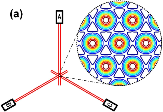
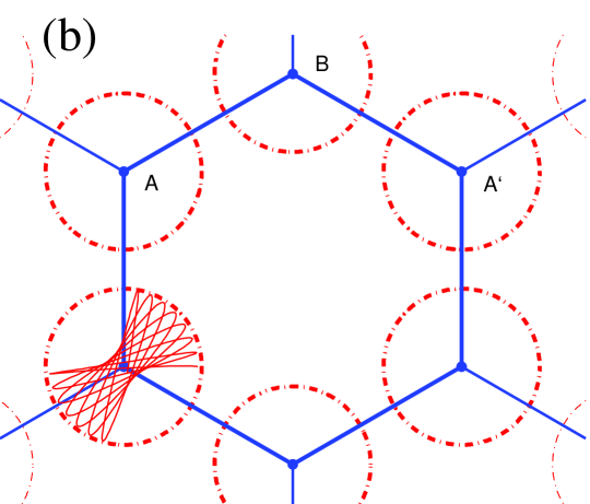
Figure 1: (Color online)  a) The sketch of the honeycomb optical lattice. The three laser beams cross each other at 120^∘ in the $xy$-plane. Phase modulators are placed in the paths of the two beams. b) The illustration of the on-site rotation by Gemelke et al. Gemelke (2007); Sarajic et al. (2009); Gemelke et al. (2010). The entire lattice takes the motions of a fast oscillation with the frequency $\omega_{\text{RF}}$ and a slow precession with the frequency $\Omega$, as schematically plotted with the red solid lines in one lattice site. After taking the time average of the fast oscillation, atoms feel that each site is rotating around its own center with the precession frequency $\Omega$, which is plotted with the red dot dash line around each site.

In this section we describe the experimental setup by Gemelke et al. to realize the on-site rotation of optical lattices Gemelke et al. (2010); Gemelke (2007); Sarajic et al. (2009), and then construct the effective tight-binding model for such a system.

II.1 The experiment setup by Gemelke et al.

The honeycomb optical lattice was experimentally realized quite some time ago Grynberg et al. (1993); Zhu et al. (2007); Lee et al. (2009); Soltan-Panahi et al. (2010). It is constructed by three phase coherent coplanar laser beams with polarization along the $z$-axis, intersecting each other with $120^{\circ}$ in the $xy$-plane. The schematic diagram of the experiment setup is shown in Fig. 1. The potential minima of the interference pattern form the honeycomb lattice if the laser frequency is blue-detuned from the atom resonance frequency. The advantage of this technique is that the phase shift in the laser beams only leads to shift entire lattices without destroying the lattice geometry.

The on-site rotation technique by Gemelke et al. was originally applied to the triangular lattice Sarajic et al. (2009); Gemelke et al. (2010). It would be straightforward to apply the same method to the honeycomb lattice. Two electro-optic modulators are placed in two of the laser beams, and the phase modulated potential is Gemelke (2007)

$$V(\vec{r}) = V_{0}[\cos(\vec{k}_{1}\cdot\vec{r}+\phi^{+})+\cos(\vec{k}_{2}\cdot\vec{r}+\phi^{-})$$ (1)

$$+ \cos(\vec{k}_{3}\cdot\vec{r}-\phi^{+}-\phi^{-})],$$

where $\vec{k}_{i}=\frac{1}{2}\epsilon_{ijk}(\vec{q}_{j}-\vec{q}_{k})$; $\vec{q}_{i}(i=1,2,3)$ are the wavevectors of the three coplanar laser beams satisfying $|q_{1}|=|q_{2}|=|q_{3}|=q$. In the following of this paper, we use the definition of recoil energy $E_{r}=\hbar^{2}q^{2}/(2M)$ where $M$ is the atom mass. Please note that this definition of $E_{r}$ is 3 times smaller than that used in Ref. Wu and Das Sarma (2008) which is defined as $\hbar^{2}k^{2}/(2M)$. In Eq. 1, $\phi^{\pm}=\eta\sin(\Omega t\pm{\frac{2\pi}{3}})\sin(\omega_{\text{RF}}t)$ where $\Omega$ is the slow precession frequency; $\eta$ is a phase modulating constant which determines the amplitude of the oscillation; $\omega_{\text{RF}}$ is the fast rotation frequency at radio frequency. Atoms do not follow the fast oscillation and only feel a time average of the potential as

$$V(\vec{r},t)=V_{0}\sum_{i=1}^{3}\big{[}A_{i}(t)\cos(\vec{k}_{i}\cdot\vec{r})\big{]},$$ (2)

where $A_{i}(t)=J_{0}[\eta\sin(\Omega t+\frac{2\pi}{3})]$; $J_{0}$ is the zeroth order Bessel function; $\eta$ is a small parameter Gemelke (2007).

Eq. 2 still maintains the same lattice translational symmetry. Around each potential minimum $\vec{r}_{0}$ in the original lattice without rotation, the potential can be expanded to the second order, yielding a slightly anisotropic harmonic potential:

$$V(\vec{r}-\vec{r}_{0},t) \approx {V_{0}\over 4}\Big{\{}\frac{8\pi^{2}}{3}\left(1-\frac{\eta^{2}}{8}\right)|\vec{r}-\vec{r}_{0}|^{2}+\frac{\eta^{2}\pi^{2}}{6}$$ (3)

$$\times \left|\vec{r}-\vec{r}_{0}\right|^{2}\cos\big{[}\frac{\pi}{3}+2(\Omega t+\varphi_{\vec{r}-\vec{r}_{0}})\big{]}\Big{\}},\ \ \$$

which rotates with a slow frequency of $\Omega$. Here $\varphi_{\vec{r}-\vec{r}_{0}}$ is the polar angle of $\vec{r}-\vec{r}_{0}$. The slight deformation of the optical potential processes around each site center, which can be regarded as an on-site rotation.

II.2 The tight-binding Hamiltonian

Now we construct the effective tight-binding model to describe the above system. First of all, each lattice site is rotating around its own center, and there is no overall rotation of the entire lattice. In other words, the system still has the lattice translational symmetry. There should be no vector potential for inter-site hopping associated with the Coriolis force. Within each site, the rotation angular velocity couples to the onsite orbital angular momentum through the orbital Zeeman coupling. Such a coupling also exists in solid state systems in the presence of external magnetic fields. However, the typical energy scales of the Zeeman couplings, including both spin and orbital channels, are at most at meV which are tiny compared to band widths. They usually do not change the band topology. The advantage of the experiments by Gemelke et al. Gemelke (2007); Sarajic et al. (2009); Gemelke et al. (2010) is that the orbital Zeeman energy scale can easily reach the order of kHz, which is comparable to band widths.

The orbital Zeeman term from the onsite rotation becomes important in orbital bands with angular momenta higher than $s$. For the $p_{x,y}$-orbital bands, one of us Wu (2008a) introduced the following coupling as

$$H_{L}=-\Omega\sum_{\vec{r}}L_{z}(\vec{r})=i\hbar\Omega\sum_{\vec{r}}\big{\{}p^{{\dagger}}_{x,\vec{r}}p_{y,\vec{r}}-p^{{\dagger}}_{y,\vec{r}}p_{x,\vec{r}}\big{\}}.$$ (4)

It breaks the degeneracy between $p_{x}\pm ip_{y}$ states, and induces topologically non-trivial band structures as presented in later sections.

The remaining part of the tight-binding Hamiltonian is as usual. In Ref Wu et al. (2007); Wu and Das Sarma (2008), one of us studied the $p_{x,y}$-orbital bands in the honeycomb optical lattice filled with spinless fermions, which is the counterpart of graphene described by the $p_{z}$-orbital but exhibits fundamentally different properties. The tight-binding Hamiltonian reads

$$H_{0} = t_{\parallel}\sum_{\vec{r}\in A}\sum^{3}_{i=1}\big{\{}p^{{\dagger}}_{i,\vec{r}}p_{i,\vec{r}+\hat{e}_{i}}+h.c.\big{\}}-\mu\sum_{\vec{r}\in A\oplus B}n(\vec{r}),~{}$$ (5)

where $\hat{e}_{1,2}=\pm\frac{\sqrt{3}}{2}\hat{x}+\frac{1}{2}\hat{y}$ and $\hat{e}_{3}=-\hat{y}$; $A$ and $B$ are indices of two different sublattices; $t_{\parallel}$ is the $\sigma$-bonding describing the longitudinal banding of $p$-orbitals along the bond direction; $\mu$ is the chemical potential; $n(\vec{r})=p^{{\dagger}}_{x,\vec{r}}p_{x,\vec{r}}+p^{{\dagger}}_{y,\vec{r}}p_{y,\vec{r}}$ is the filling number at site $\vec{r}$. The operators $\hat{p}_{i,\vec{r}}$ are defined as the projection of $p$-orbital along the vector $\hat{e}_{i}$ as $\vec{p}_{\vec{r}}=p_{x,\vec{r}}\hat{x}+p_{y,\vec{r}}\hat{y}$. Rigorously speaking, $t_{\parallel}$ should be time-dependent which depends on the oscillation amplitude $\eta$. Here we neglect this time-dependence by assuming $\eta$ is small. $t_{\parallel}$ is positive as a result of the odd parity of the $p$ -orbitals. The $\pi$-bonding $t_{\perp}$ is much weaker than the $\sigma$-bonding. For example, $t_{\perp}/t_{\parallel}$ can be easily suppressed around $1\%$ Wu (2008a) within realistic experimental parameters of $V_{0}/E_{r}=15$, thus the $t_{\perp}$ is not considered in most of this paper unless in Sect. IV.3. The band Hamiltonian to be investigated below is the combination between Eq. 4 and Eq. 5 as

$$H=H_{0}+H_{L}.$$ (6)

III The appearance of the Haldane model at large rotation angular velocities

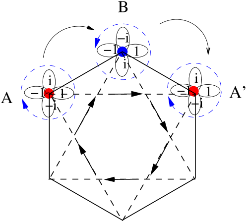
Figure 2: (Color online) The pattern of the induced complex-valued NNN hopping at $\Omega\gg t_{\parallel}$, which is generated by the virtual hopping between orbitals with opposite chiralities. From Wu Wu (2008a).

Haldane proposed a tight-bonding model for the QAHE effect whose Bloch wave band structure is topologically non-trivial Haldane (1988). The Hamiltonian of the Haldane model is defined in the honeycomb lattice, which reads

$$H=-t\sum_{\langle ij\rangle}\Big{\{}a^{{\dagger}}_{i}a_{j}+h.c.\Big{\}}+\sum_{\langle\langle ij\rangle\rangle}\Big{\{}t^{\prime}_{ij}a^{{\dagger}}_{i}a_{j}+h.c.\Big{\}},$$ (7)

where $\langle ij\rangle$ represents the nearest-neighbor (NN) hopping; $\langle\langle ij\rangle\rangle$ represents the next-nearest-neighbor (NNN) hopping. The NNN hopping $t^{\prime}=|t^{\prime}|e^{\pm i\phi}$ is complex-valued whose argument takes $\pm\phi$ if the hopping from $i$ to $j$ is anticlockwise (clockwise) with respect to the plaquette center. Eq. 7 breaks time-reversal symmetry. The band spectra exhibit two gapped Dirac cones in the Brillouin zone (BZ), whose mass values have opposite signs. The band structure has the non-vanishing Chern numbers $\pm 1$, which leads to the QAHE with $\nu=\pm 1$. In the system with the open boundary conduction, unidirectional edge currents appear surrounding the system, i.e., the edge currents are chiral.

Before the detailed study on the band structures of our $p$-orbital Hamiltonian Eq. 6, we present an intuitive picture that the on-site rotation induces complex-valued NNN hopping terms in the limit of $\Omega/t_{\parallel}\gg 1$ as in the Haldane model. As a result, the Gemelke type rotation provides a possibility to realize the QAHE state in the cold atom experiments. In the presence of rotation, the on-site eigen-orbitals become $p_{x}\pm ip_{y}$ with an energy splitting of $2\Omega$. When $\Omega\gg t_{\parallel}$, each level of $p_{x}\pm ip_{y}$ broadens into a band without overlapping each other. We consider the case that $\Omega>0$, such that the low energy sector of the Hilbert space consists of the $p_{x}+ip_{y}$ orbital state. The leading order term of the effective Hamiltonian in this sector is just the NN hopping with the hopping integral of $\frac{1}{2}t_{\parallel}$. Moreover, the second order perturbation process generates the NNN hopping with complex-valued integral as explained below.

Let us consider the two-step virtual hopping process illustrated in Fig. 2. In the first step, the atom starting from the low energy sector of the $p_{x}+ip_{y}$ orbital in the A-site hops into the high energy sector of the $p_{x}-ip_{y}$ orbital in the nearest neighbor B-site. The phases along the AB-bond is $30^{\circ}$ from the A-site and $150^{\circ}$ from the B-site, thus there is a phase mismatch of $120^{\circ}$. The corresponding hopping integral is complex-valued with $\frac{1}{2}t_{\parallel}e^{i\frac{2}{3}\pi}$. Similarly, during the second step the atom hops back into the $p_{x}+ip_{y}$ orbital in the NNN A-site with the complex hopping integral $\frac{1}{2}t_{\parallel}e^{i\frac{2}{3}\pi}$. The hopping process is $(A+)\to(B-)\to(A^{\prime}+)$ where $\pm$ represents the chirality of $p_{x}\pm ip_{y}$ orbitals. The corresponding amplitude is calculated as follows:

$$t_{\text{NNN}} = \frac{\langle A^{\prime}+|H_{0}|B-\rangle\langle B-|H_{0}|A+\rangle}{-2\Omega}$$ (8)

$$= -{\frac{t_{{\small\parallel}}^{2}}{8\Omega}}e^{i4\pi/3}.\ \ \$$

All the NNN hoppings have the same phase value following the arrows, which is exactly the same as in the Haldane model. The above analysis applies to the high energy sector as well. Thus we have two copies of the Haldane model, each for the $p_{x}\pm ip_{y}$ bands, respectively.

IV Band structures in the homogeneous system

In this section, we present the band spectra in the homogeneous system with the periodical boundary conditions (PBC). The general structure is studied in Sec. IV.1, and the interesting flat band structure is presented in Sec. IV.2.

IV.1 The general band structures

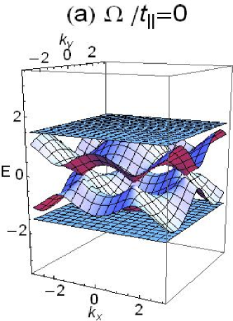
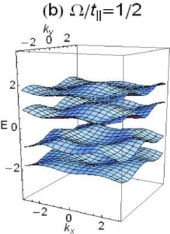
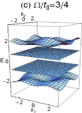
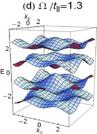
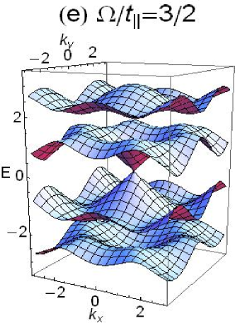
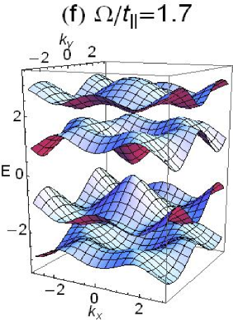
Figure 3: (Color online)  The band structures of the Hamiltonian Eq. [15]. With increasing rotation velocity from (a) $\Omega/t_{\parallel}=0$ to (f) $\Omega/t_{\parallel}=1.7$. The flat bands appear at $\Omega/t_{\parallel}=\frac{3}{4}$. Energies are in unit of hopping strength $t_{\parallel}$ and wavevectors are in the unit of $1/a$, which is the reciprocal of the lattice constant. The energies of these two flat bands are $E/t_{\parallel}=\pm\frac{3}{4}$.

We define the four-component spinor representation for the two-orbital wavefunctions in the two sublattices as

$$|\psi_{\vec{k}}\rangle=\left[p_{Ax}(\vec{k}),p_{Ay}(\vec{k}),p_{Bx}(\vec{k}),p_{By}(\vec{k})\right]^{T}.$$ (9)

After performing the Fourier transform, the Hamiltonian Eq. 6 becomes

$$H=\sum_{\vec{k}}\psi^{{\dagger}}_{a}(\vec{k})[H_{ab}(\vec{k})-\delta_{ab}\mu]\psi_{b}(\vec{k}),$$ (10)

where $H_{ab}(\vec{k})$ is written as

$$\left(\begin{array}[]{cccc}0&i\Omega&\frac{3}{4}(e^{i\vec{k}\cdot\vec{e}_{1}}+e^{i\vec{k}\cdot\vec{e}_{2}})&\frac{\sqrt{3}}{4}(e^{i\vec{k}\cdot\vec{e}_{1}}-e^{i\vec{k}\cdot\vec{e}_{2}})\\ -i\Omega&0&\frac{\sqrt{3}}{4}(e^{i\vec{k}\cdot\vec{e}_{1}}-e^{i\vec{k}\cdot\vec{e}_{2}})&\frac{1}{4}(e^{i\vec{k}\cdot\vec{e}_{1}}+e^{i\vec{k}\cdot\vec{e}_{2}})+e^{i\vec{k}\cdot\vec{e}_{3}}\\ h.c.&&0&i\Omega\\ &&-i\Omega&0,\end{array}\right).$$ (15)

The band structure in the absence of rotation i.e., $\Omega=0$, has been studied in Ref. Wu et al. (2007); Wu and Das Sarma (2008), which includes both flat bands (the bottom and top bands) and two dispersive bands with Dirac cones as depicted in Fig. 3 (a). The flat bands and dispersive bands touch at the center of the first BZ, and two dispersive bands touch at Dirac cones. The location of the Dirac cones are at $\vec{k}=(\pm\frac{4\pi}{3\sqrt{3}a},0)$ Wu et al. (2007); Wu and Das Sarma (2008). The band flatness means that the corresponding band eigenstates can be constructed as localized states in real space. Each hexagonal plaquette supports one localized eigenstate whose orbital configuration on each site is along the tangent direction as presented in Fig. 2a in Ref. Wu et al. (2007). When the filling is inside the flat bands, interaction effects are non-perturbative. This results in the exact solutions of the Wigner crystallization for spinless fermions Wu et al. (2007) and the flat band ferromagnetism for spinful fermions Zhang et al. (2010). For the dispersive bands, although their spectra are the same as in graphene, their eigen-wavefunctions are fundamentally different exhibiting rich orbital structures as presented in Ref. Wu and Das Sarma (2008).

When the on-site rotation is turned on, i.e., $\Omega>0$, band gaps open. The previous touching points between the first and second bands at $\Omega=0$ split. The lowest band is no longer flat, and the center of the second band is pushed up as depicted in Fig. 3 (b). The Dirac cones between the middle two dispersive bands also become gapped. In this case, the topology of each band $n~{}(n=1\sim 4)$ is characterized by the Chern number defined as

$$C_{n}=\frac{1}{2\pi}\int d^{2}k~{}F_{n,xy}(\vec{k}),$$ (16)

where the Berry curvature $F_{n,xy}$ is defined as

$$F_{n,xy}(\vec{k})=\partial_{k_{x}}A_{n,y}(\vec{k})-\partial_{k_{y}}A_{n,x}(\vec{k}),$$ (17)

and $A_{n,\mu}(\mu=x,y)$ is the Berry gauge potential in momentum space defined as

$$A_{n,\mu}=i\langle\psi_{n}(\vec{k})|\partial_{k_{\mu}}|\psi_{n}(\vec{k})\rangle.$$ (18)

The Chern number patterns at $\Omega>0$ have been calculated in Ref. Wu (2008a), and the distribution of the Berry curvatures $F_{n,xy}$ in the BZ is depicted in Fig. 2 of Ref. Wu (2008a). Below a critical value of the rotation angular velocity $\Omega_{c}/t_{\parallel}=\frac{3}{2}$, the Chern number pattern reads

$$C_{1}=-C_{4}=1;~{}~{}~{}C_{2}=-C_{3}=0.$$ (19)

At $\Omega_{c}/t_{\parallel}=\frac{3}{2}$, a single Dirac cone connecting the second and third bands shows up at $\vec{k}=(0,0)$, which triggers a topological phase transition. Beyond $\Omega_{c}$, this Dirac point becomes gapped, and the Chern number pattern becomes

$$C_{1}=-C_{2}=1;~{}~{}~{}C_{3}=-C_{4}=-1.$$ (20)

In this case, the band structure is qualitatively the same as the two copies of the Haldane model as discussed in Sec. III.

IV.2 Flat bands at $\Omega/t_{\parallel}=\frac{3}{4}$

It is evident in Fig. 3 (c) that the second and third bands become flat at $\Omega/t_{\parallel}=\frac{3}{4}$. In this part, we discuss various properties of the flat bands, including the localized eigen-states, the distribution of the Berry curvature, and the interaction effects.

IV.2.1 Localized eigen-states

The band flatness usually means that the eigen-states can be reconstructed as localized states in real space. We assume that each localized eigenstate exists within a single hexagon plaquette constructed as follows

$$|\psi_{\vec{R}}\rangle=\sum_{j=1}^{6}(-)^{j-1}e^{i(j-1)\phi}\Big{\{}\cos\theta_{j}|p_{j,x}\rangle-\sin\theta_{j}|p_{j,y}\rangle\Big{\}},\ \ \$$ (21)

where $\vec{R}$ is the coordinate of the plaquette center; $j$ is the site index within the same plaquette and $\theta_{j}=(j-1)\frac{\pi}{3}$; $e^{i\phi}$ is the phase factor to be determined satisfying the periodical boundary condition $e^{i6\phi}=1$; the factor of $(-)^{j-1}$ is a sign convention because of the odd parity of the $p$-orbitals. The $p$-orbital configuration on each site $j$ is along the tangent direction. Substituting Eq. 21 into the band Hamiltonian, we arrive at the condition for Eq. 21 to be the eigenstate as

$$\Omega=-{\frac{\sqrt{3}}{2}}\sin{\phi},\ \ \,E=-{\frac{3}{2}}\cos{\phi},$$ (22)

where $\phi=0,\pm\frac{\pi}{3},\pm\frac{2\pi}{3},\pi$. For the cases of $\phi=0$ and $\pi$, they are the situations studied before in Ref. Wu et al. (2007) without the on-site rotation. The other four cases are with the on-site rotation. Without loss of any generality, we take $\phi=-\frac{\pi}{3}$ and $\phi=-\frac{2\pi}{3}$ such that $\Omega/t_{\parallel}=\frac{3}{4}>0$ and $E/t_{\parallel}=\pm\frac{3}{4}$. The schematic diagram of these two typical localized state is shown in Fig. 4 (a) and (b), respectively.

The main difference between these two groups of localized states at $\Omega=0$ and $\Omega/t_{\parallel}=\frac{3}{4}$ is that there exists a current around each plaquette for the latter case. The current operator along each bond is defined as

$$\hat{J}_{\vec{r},\vec{r}^{+}\hat{e}_{i}}=i\frac{t_{\parallel}}{\hbar}\Big{\{}\hat{p}^{\dagger}_{\vec{r}}\cdot\hat{e}_{i})(\hat{p}_{\vec{r}+\hat{e}_{i}}\cdot\hat{e}_{i})-h.c.\Big{\}}.$$ (23)

For the localized plaquette eigen-states of both bands with $E=\pm\frac{3}{4}t_{\parallel}$, the currents have the same value and chirality as

$$J=-\sqrt{3}\Omega.$$ (24)

Eq. 24 indicates that the current direction is opposite to the rotation and the magnitude is proportional to the angular velocity $\Omega$.

At $\Omega/t_{\parallel}=\frac{3}{4}$, we solve the eigenvectors for the two flat bands in momentum space as

$$|\psi_{\vec{k},\mp}\rangle=\frac{1}{\sqrt{N_{\mp}(\vec{k})}}\left(\begin{array}[]{c}\frac{1}{2}e^{-ik\cdot e_{1}\mp i\chi_{1}}+\frac{1}{2}e^{-ik\cdot e_{2}\mp i\chi_{2}}-e^{-ik\cdot e_{3}\mp i\chi_{3}}\\ \frac{\sqrt{3}}{2}e^{-ik\cdot e_{1}\mp i\chi_{1}}-\frac{\sqrt{3}}{2}e^{-ik\cdot e_{2}\mp i\chi_{2}}\\ \pm(\frac{1}{2}e^{ik\cdot e_{1}\mp i\chi_{1}}+\frac{1}{2}e^{ik\cdot e_{2}\mp i\chi_{2}}-e^{ik\cdot e_{3}\mp i\chi_{3}})\\ \mp(\frac{\sqrt{3}}{2}e^{ik\cdot e_{1}\mp i\chi_{1}}-\frac{\sqrt{3}}{2}e^{ik\cdot e_{2}\mp i\chi_{2}})\end{array}\right),$$ (29)

where $\psi_{\mp}(\vec{k})$ represent eigenvectors for the bands with $E/t_{\parallel}=\mp\frac{3}{4}$, respectively; $\chi_{1}={\frac{\pi}{6}},\chi_{2}={\frac{5\pi}{6}}$, and $\chi_{3}={\frac{3\pi}{2}}$. The normalization factors $N_{\mp}(\vec{k})$ read

$$N_{\mp}(\vec{k})=2\Big{[}3-\sum_{i}\cos(\vec{k}\cdot\vec{b}_{i}\mp\frac{2}{3}\pi)\Big{]}.$$ (30)

These flat band Bloch wave states can be represented as the linear superpositions of the localized eigenstates in Eq. 21 as :

$$|\psi_{\vec{k},\mp}\rangle={\frac{1}{\sqrt{N_{\mp}(\vec{k})}}}\sum_{\vec{R}}e^{i\vec{k}\cdot\vec{R}}|\psi_{R}\rangle$$ (31)

where $|\psi_{R}\rangle$ is defined in Eq. 21.

IV.2.2 Brief discussions on interaction effects

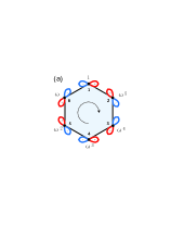
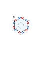
Figure 4: (Color online)  Configurations of the localized eigenstates of the two flat bands at $\Omega/t_{\parallel}=\frac{3}{4}$ for (a) $E/t_{\parallel}=-\frac{3}{4}$ and (b) $E/t_{\parallel}=\frac{3}{4}$, respectively. $\omega=e^{i\frac{\pi}{3}}$ is the relative phase factor between neighboring sites. The plaquette currents directions are clockwise for both (a) and (b) in the opposite direction of the $\Omega$.

The band flatness means that interaction effects are always important compared to the vanishing kinetic energy scale. In our previous studies Wu et al. (2007); Wu and Das Sarma (2008); Zhang et al. (2010), we have examined the non-perturbative effects in the flat bands (the lowest and highest bands) in the same system at $\Omega=0$. In Ref. Wu et al. (2007); Wu and Das Sarma (2008), we have shown that the flat bands result in the exact solution of Wigner crystal configuration for spinless fermions in the lowest band. At $\langle n\rangle=\frac{1}{6}$, which corresponds to that $\frac{1}{3}$ of the flat band plaquette states are occupied, the occupied plaquettes form a triangular lattice structure without touching each other. As filling increases, exact solutions are no longer available. Self-consistent mean-field theory calculation shows a serials of insulating states with different orbital orderings at commensurate fillings Wu and Das Sarma (2008). Similarly, in Ref. Zhang et al. (2010), we found the exact flat-band ferromagnetism for spinful fermions in the flat bands.

For the flat bands occurring at $\Omega/t_{\parallel}=\frac{3}{4}$, the physics will be similar to the previous studies at $\Omega=0$. However, the flat bands here are in the middle. When $\mu$ lies in the flat bands, there are always background particles or holes filling in the dispersive bands. The solutions of the Wigner crystal and flat-band ferromagnetism is only valid if the interaction energy scale is smaller than the band gaps between the flat bands and the dispersive bands. For example, when the filling is inside the second band, the effect from the background filling cannot be neglected, if the interaction energy scale is stronger than the band gap.

IV.2.3 Berry curvatures v.s. local eigen-states

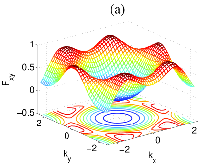
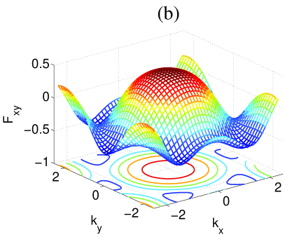
Figure 5: (Color online)   The Berry curvature $F_{xy}$(in unit of $a^{2}$) distribution at $\Omega/t_{\parallel}=\frac{3}{4}$ for the 1st (a) and 2nd (b) bands. The Chern numbers for the 1st and 2nd bands are 1 and 0, respectively. The unit of wave vector is $1/a$.

The current carried by the localized eigenstates of the flat bands depicted in Fig. 4 is chiral. It looks very similar to the classic picture of cyclotron orbit of electrons in the external magnetic fields. We would expect that in a system with the open boundary condition, the fully filled flat band would result in edge currents and contributes to the quantized anomalous Hall conductance. However, we need to be very careful with this, which turns out to be incorrect. We have performed a preliminary diagonalization for a finite size system with the open boundary condition. The number of degeneracy for the flat bands equals to the number of plaquettes plus 1. We conjecture that this extra state should not belong to a particular plaquette but rather distribute along the edge, which carries a current in the opposite direction and cancels the contribution from other plaquette states. Further examinations on this problem will be deferred to a later publication.

We calculate the Berry curvature distributions at $\Omega/t_{\parallel}=\frac{3}{4}$ for the 1st and 2nd bands as presented in Fig. 5 (a) and (b), respectively. Those of the 3rd (4th) band are just with an opposite sign compared to the 2nd (1st) band due to the particle-hole symmetry of the band Hamiltonian. The 1st and 4th bands are topologically non-trivial with the Chern number $\pm 1$. However, the 2nd and 3rd bands, which are flat, are topologically trivial with the zero Chern number. In fact, these two bands should not contribute to quantum anomalous Hall conductance when they are fully filled. This is confirmed from the anomalous Hall current calculation in the inhomogeneous trap as presented in Sec. V.

IV.3 Effects of the $\pi$-bonding to band structures

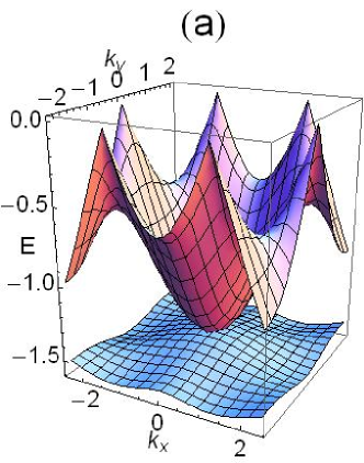
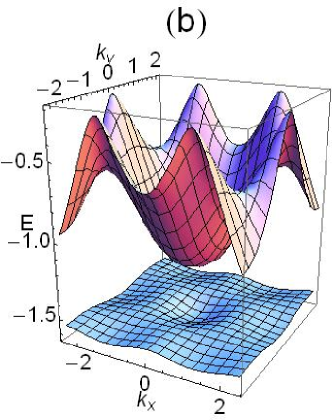
Figure 6: (Color online)   The band structures with both $\pi$-bonding $(t_{\perp}/t_{\parallel}=0.05)$ and on-site rotation $\Omega$. Only the lower two bands are presented, and the spectra of the other two bands are symmetric with respect to zero energy. (a) At $\Omega/t_{\parallel}=0$, the two bands remain touching at the center of the BZ. The lowest band develops dispersion at the order of $t_{\parallel}$. (b) At $\Omega/t_{\parallel}=0.2$, the gap opens between the lower two bands. The lowest band is topologically non-trivial and nearly flat.

So far, we have neglected $\pi$-bonding $t_{\perp}$ which can be easily suppressed around $1\%$ of $t_{\parallel}$ at intermediate optical potential strength Wu and Das Sarma (2008). Here we explicitly present its effects to band structures for the case of a realtively weak lattice potentials by taking $t_{\perp}/t_{\parallel}=0.05$. The projections of $p_{x,y}$-orbitals perpendicular to the $\hat{e}_{1,2,3}$ directions are defined as $p^{\prime}_{1,2}=-\frac{1}{2}p_{x}\pm\frac{\sqrt{3}}{2}p_{y},p^{\prime}_{3}=p_{x}$, respectively. The $\pi$-bonding Hamiltonian can be written as

$$H_{\pi} = -t_{\perp}\sum_{\vec{r}\in A,i=1\sim 3}\Big{\{}p^{\prime\dagger}_{\vec{r},i}p^{\prime}_{\vec{r}+a\hat{e}_{i},i}+h.c.\Big{\}},$$ (32)

where the hopping integral of the $\pi$-bonding has the opposite sign to that of the $\sigma$-bonding. In momentum space, Eq. 32 transforms into

$$H_{\pi} = -t_{\perp}\sum_{k}\psi^{\dagger}_{\alpha}(\vec{k})H_{\pi,\alpha\beta}(\vec{k})\psi_{\beta}(\vec{k}),$$ (33)

with the martix kernel $H_{\pi}(\vec{k})$ as

$$\left(\begin{array}[]{cccc}0&0&\frac{1}{4}(e^{i\vec{k}\cdot\hat{e}_{1}}+e^{i\vec{k}\cdot\hat{e}_{2}})+e^{i\vec{k}\cdot\hat{e}_{3}}&\frac{3}{4}(-e^{i\vec{k}\cdot\vec{e}_{1}}+e^{i\vec{k}\cdot\hat{e}_{2}})\\ 0&0&\frac{3}{4}(-e^{i\vec{k}\cdot\vec{e}_{1}}+e^{i\vec{k}\cdot\vec{e}_{2}})&\frac{\sqrt{3}}{4}(e^{i\vec{k}\cdot\vec{e}_{1}}+e^{i\vec{k}\cdot\vec{e}_{2}})\\ h.c.&&0&0\\ &&0&0\end{array}\right).$$ (38)

The effects of $\pi$-bonding $t_{\perp}$ are presented in Fig. 6. The spectra remain symmetric with respect to zero energy, and thus only the lower two bands are presented. As presented in Ref. Wu and Das Sarma (2008), at $\Omega=0$, the bottom bands are no longer rigorously flat but develops a finite width at the order of $t_{\perp}$. The lower two bands remain touching at $\vec{k}=(0,0)$ with parabolic spectra, and the bottom band has a negative curvature. With increasing $\Omega$, as in the case of $t_{\perp}=0$, the band gap at the order of $\Omega$ opens. Furthermore, $\Omega$ lowers the energies of the bottom band near the center of the BZ, which suppresses its dispersion. As a result, we arrive at a nearly flat band with non-zero Chern number. The ratio between the width of the bottom band and the gap between the lower two bands can reach the order of 5 as shown in Fig. 6 b. Recently, we notice that the nearly flat bands with non-trivial Chern number have been attracting attention, for its possible realization of fraction quantum Hall states in the lattice Sun et al. (2010); Neupert et al. (2010); Tang et al. (2010).

V Anomalous Hall currents in harmonic trap potentials

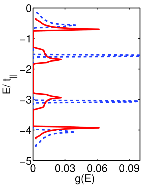
Figure 7: (Color online)  The DOS of the $p_{x,y}$-orbital model Eq. 5 and Eq. 4 in the homogeneous system. The red solid lines are the DOS at $\Omega/t_{\parallel}=\frac{1}{2}$ whereas the blue dash lines are the DOS at $\Omega/t_{\parallel}=\frac{3}{4}$.

In section IV, the homogeneous $p$-orbital system with the PBC has been studied, in which the wavevector $k$ is a good quantum number. However, in reality the honeycomb lattice is inhomogeneous with a soft harmonic confining trap. In this section, we shall consider the anomalous Hall currents in such a realistic system.

The trapping potential adds a new term in the band Hamiltonian $H_{0}+H_{L}$ of Eqs. 5 and 4 as

$$H_{T}=\sum_{\vec{r}}V_{T}(r)n(\vec{r}).$$ (40)

The trapping potential $V_{T}(r)$ reads

$$V_{T}(r)=\frac{1}{2}M\omega_{T}^{2}r^{2}=\frac{\beta t_{\parallel}}{2}\big{(}\frac{r}{a}\big{)}^{2},$$ (41)

where $a$ is the lattice constant, $\beta=\frac{\hbar\omega_{T}}{t_{\parallel}}(\frac{a}{l_{0}})^{2}$; $l_{0}=\sqrt{\frac{\hbar}{M\omega_{T}}}$ is the trapping length scale. The typical value of the trapping frequency $\omega_{T}$ is in the order of 10Hz, and that of the recoil energy $E_{r}$ is roughly several kHz Leggett (2001). In Ref. Wu and Das Sarma (2008), we have calculated that $t_{\parallel}/E_{r}=0.24$ for $V_{0}/E_{r}=15$, thus $\hbar\omega/t_{\parallel}$ is at the order of 0.1. The typical trapping length scale is several lattice constants. Taking into account all these factors, we choose a convenient value of $\beta=0.01$ for later calculations.

In the inhomogeneous system with trapping potential, the on-site rotation induces the circulating currents along the azimuthal direction. We will study the spatial distributions of the these anomalous Hall currents and particle density. Because the band topology has a transition at $\Omega_{c}/t_{\parallel}=\frac{3}{2}$, the results are presented at different sets of parameters below, at, and above $\Omega_{c}$. Our results are calculated by using the eigen-wavefunctions from the numerical diagonalization of the free Hamiltonian in an open lattice with the trapping potential. We also use a modified local-density-approximation (LDA) to understand the exact results. The size of the lattice is with the radius of $r/a=40$.

V.1 Low rotation angular velocity

In this subsection the angular velocities are taken as $\Omega/t_{\parallel}=\frac{1}{2}$ and $\frac{3}{4}$ below $\Omega_{c}$. The chemical potential is chosen as $\mu/t_{\parallel}=2.3$ to guarantee that all bands are filled at the center of the trap. The spatial distribution of the particle density exhibits a four-layered wedding cake-like structure. The density plateaus correspond to the band insulating regions, where the local chemical potential, defined as $\mu_{loc}(r)=\mu-V_{T}(r)$, lies inside band gaps. Furthermore, the anomalous Hall currents flow along the tangent direction, whose conductances are quantized in the insulating regions.

V.1.1 The insulating plateaus of $\langle n(r)\rangle$

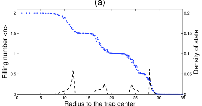
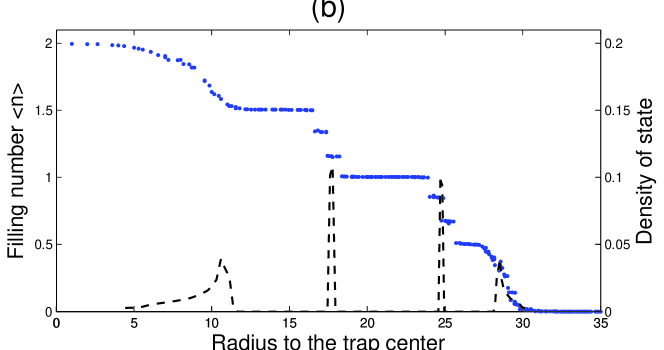
Figure 8: (Color online) The particle density distributions $\langle n(\vec{r})\rangle$ v.s. the radius $r$ at (a) $\Omega/t_{\parallel}=\frac{1}{2}$ and (b) $\frac{3}{4}$, which exhibit a four-layer wedding cake shape (the blue dots). The radius is in the unit of the lattice constant $a$. The DOS at the local chemical potential $\mu_{loc}(r)$ in the LDA approximation is plotted with the black dash lines. $\mu_{loc}(r)/t_{\parallel}=2.3$ at the center of the trap and $\omega_{T}/t_{\parallel}=0.1$.

We first present the density of states (DOS) for the $p$-orbital bands in the homogeneous system at $\Omega/t_{\parallel}=\frac{1}{2}$, and $\frac{3}{4}$ in Fig. 7. The DOS is defined as

$$g(E)=\int\frac{d^{2}k}{(2\pi)^{2}}\delta(E(\vec{k})-E).$$ (42)

At $\Omega/t_{\parallel}=\frac{3}{4}$, the strong divergence of the DOS is indicated at the 2nd and 3rd bands due to the appearance of the flat bands. At the small value of $\Omega/t_{\parallel}=\frac{1}{2}$, the DOS of the 1st and 4th bands are larger than the 2nd and 3rd bands, which is a reminiscence of the band flatness at $\Omega=0$. Moreover, it is obvious that the band gaps open at $\Omega_{c}>0$. For the chemical potential $\mu$ lying in the band gaps, the system is in the band insulating states with the commensurate values of the particle number per site $\langle n\rangle=\frac{1}{2},1,\frac{3}{2}$, and $2$, respectively.

In the inhomogeneous trap, the real space distributions of the filling number $\langle n(\vec{r})\rangle$ are calculated by using the eigenstate wavefunction obtained through diagonalizing the Hamiltonian, which are depicted in Fig. 8 for $\Omega/t_{\parallel}=\frac{1}{2}$ and $\frac{3}{4}$. In both cases, plateaus appear at $\langle n\rangle=\frac{1}{2},1,\frac{3}{2}$. These plateaus can be understood within the LDA picture. Recall the band structure in Fig. 3 and the DOS in Fig. 7. When $\mu_{loc}(r)$ lies in the band gaps, the filling number stops increasing until $\mu_{loc}(r)$ reaches next band edge. The local DOS at site $\vec{r}$ at the energy $\mu_{loc}(r)$ is also plotted, which roughly proportional to $\partial_{r}n(r)$. It is clear that the locations of the plateaus of $\langle n(r)\rangle$ are and band gaps are consistent.

Because the honeycomb lattice breaks the $SO(2)$ rotational symmetry down to the 6-fold one, lattice sites with the same magnitude of $r$ may have different values of $\langle n(r)\rangle$. They are slightly scattered in the metallic regions between different plateaus as depicted in Fig. 8 (a) and (b). In the case of $\Omega/t_{\parallel}=\frac{3}{4}$, the distribution of $\langle n(r)\rangle$ exhibit devil’s stair-like features Bak (1982, 1986). In the cliffs as filling in the middle two flat bands whose degeneracies are slightly lifted by the potential gradient. If with interactions, the flat band regime may further exhibit plateaus of Mott-insulating states with orbital orderings, which will be deferred to a later research.

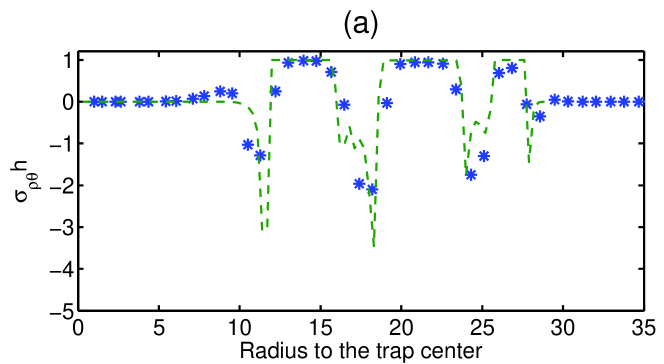
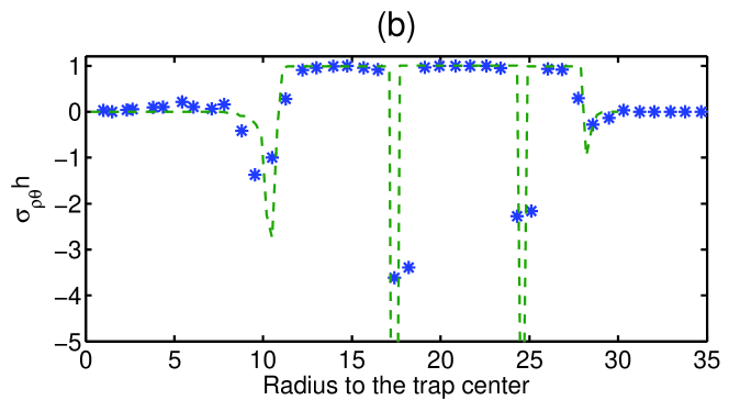
Figure 9: (Color online)   The effective local Hall conductance $\sigma_{\rho\theta}(r)$ v.s. $r$ defined in Eq. 44 at $\Omega/t_{\parallel}=\frac{1}{2}$ (a) and $\frac{3}{4}$ (b). The radius is in the unit of the lattice constant $a$. The results from diagonalizing the free Hamiltonian with the trapping potential is marked with asterisks, and those from the modified LDA are plotted with dashed lines. $\sigma_{\rho\theta}$ is quantized in the insulating plateaus with commensurate fillings of $\langle n(r)\rangle$.

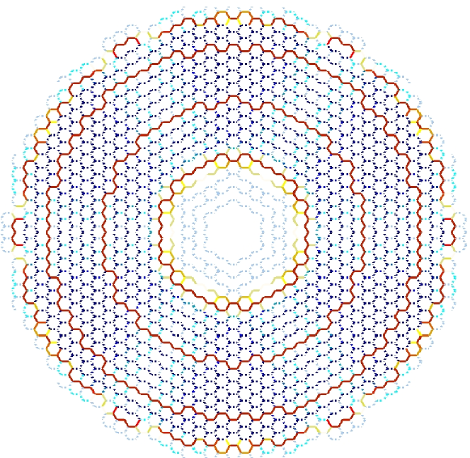
Figure 10: (Color online)   The pattern of the anomalous Hall current in the honeycomb lattice with the confining trap at the rotation of $\Omega/t_{\parallel}=0.75$. The blue dotted (red solid) lines represent the counterclockwise (clockwise) anomalous Hall currents, respectively. The color depth indicates the magnitude of the current. The reversed direction of the anomalous Hall currents (red solid lines) in the metallic regions between two neighboring plateaus can be explained as the anomalous contribution from the gradient of $\langle n(r)\rangle$.

V.1.2 QAHE currents in the insulating density plateaus

Due to the non-trivial topology of the band structure, anomalous Hall currents circulate along the azimuthal direction due to the radial potential gradient. The plateaus of the filling number $\langle n(r)\rangle$ correspond to the insulating quantum anomalous Hall regions with quantized Hall conductance. Compared with the usual quantum Hall systems, the on-site rotation breaks time-reversal symmetry and brings non-trivial topology to the band structures without Landau levels.

The anomalous Hall current along each bond is calculated by using the eigen-wavefunctions obtained from the diagonalization of the real space $p$-orbital Hamiltonian as

$$J_{\vec{r},\vec{r}^{+}\hat{e}_{i}}=i\frac{t_{\parallel}}{\hbar}\sum_{n}\langle|(\hat{p}^{\dagger}_{\vec{r}}\cdot\hat{e}_{i})(\hat{p}_{\vec{r}+\hat{e}_{i}}\cdot\hat{e}_{i})-h.c.|\rangle,$$ (43)

where $\langle||\rangle$ represents the ground state at $T=0$ or thermal average at finite temperatures. Let us focus on those bonds orienting along the azimuthal direction, and define the effective local Hall conductance as

$$\sigma_{\rho\theta}^{\text{eff}}(r)=-{j_{\theta}\over\partial_{r}V_{T}},$$ (44)

where $r$ is the radius of the middle point of the bond; $j_{\theta}$ is the current density; $V_{T}$ is the trapping potential. In our honeycomb lattice system, the current density is defined as the current on each bond $J_{\vec{r},\vec{r}^{+}\hat{e}_{i}}$ divides the distance between neighboring parallel bonds.

In the homogeneous systems, the Hall conductance is represented as

$$\sigma_{\rho\theta}=\frac{1}{h}\frac{1}{2\pi}\sum_{i}\int\mathrm{d}^{2}kF_{i,xy}(\vec{k})n_{f}(i,k),$$ (45)

where $n_{f}$ is the Fermi distribution function; $i$ is the band index. When the chemical potential is inside band gaps, $\sigma_{\rho\theta}$ is quantized as the sum of the Chern numbers of the occupied bands Xiao et al. (2009); Thouless et al. (1982); Kohmoto (1985)

$$\sigma_{\rho\theta}=\frac{1}{h}\sum_{i}C_{i}.$$ (46)

For the cases of $\Omega/t_{\parallel}=\frac{1}{2},\frac{3}{4}$, the Chern number pattern is the same as $C_{1}=-C_{4}=1$ and $C_{2}=-C_{3}=0$ Wu (2008a). The quantized Hall conductances reads $0$, $1$, $1$ and $1$ as $\mu$ lies from above the band top down to the three consecutive three band gaps.

The results of $\sigma_{\rho\theta}^{\text{eff}}(r)$ (defined in Eq. 44) v.s $r$ are marked as asterisks in Fig. 9 (a) and (b) for $\Omega/t_{\parallel}=\frac{1}{2}$ and $\frac{3}{4}$, respectively, which are obtained by diagonalizing the free but inhomogeneous Hamiltonian. The real space circulating current pattern at $\Omega/t_{\parallel}=\frac{3}{4}$ is depicted in Fig. 10. The quantized Hall conductances in the insulating plateau regions can be understood within the LDA picture. At the center, the local chemical potential $\mu_{loc}(r)$ lies above the band top, and the conductance is therefore zero. As moving into the insulating density plateaus of $\langle n(r)\rangle=\frac{3}{2},1$, and $\frac{1}{2}$, $\sigma^{\text{eff}}_{\rho\theta}$ is quantized at $1/h$. Counterclockwise currents are plotted as blue dash line under the harmonic trap potential. When the radius $r>30$, the Fermi level is lower than the band bottom, thus the current vanishes again.

V.1.3 Anomalous Hall currents in the metallic regions

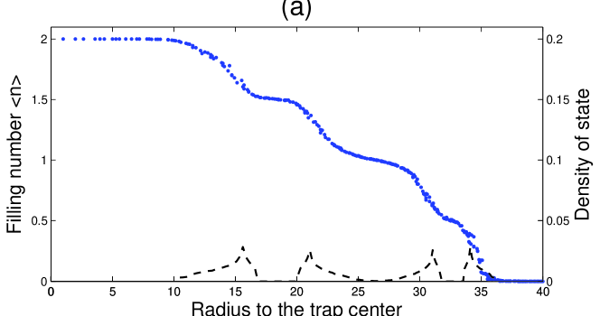
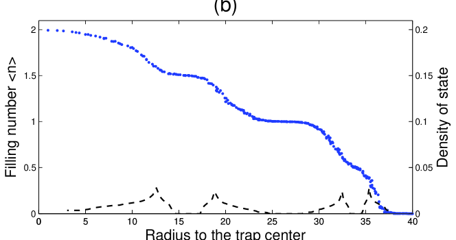
Figure 11: (Color online)  The particle density distributions $\langle n(\vec{r})\rangle$ v.s. the radius $r$ at (a) $\Omega/t_{\parallel}=\frac{3}{2}$ and (b) $2$ (the blue dots). The radius is in the unit of the lattice constant $a$. The DOS at the local chemical potential $\mu_{loc}(r)$ in the LDA approximation is plotted with the black dash lines. $\mu_{loc}(r)/t_{\parallel}=3.5$ at the center of the trap and $\omega_{T}/t_{\parallel}=0.1$.

Between two adjacent insulating plateaus, the system is metallic with incommensurate fillings of $\langle n(r)\rangle$, therefore the anomalous Hall conductances are non-quantized. The Hall current response to the radial potential gradient is non-local in these inhomogeneous metallic regions. The effective Hall conductance $\sigma_{\rho\theta}$ defined in Eq. 44 cannot be obtained from Eq 45 of the homogeneous system by using LDA with a local chemical potential $\mu_{loc}(r)$. For example, the currents can reverse the direction to be clockwise in the metallic regions in Fig. 9 (a) and (b). However, because of the Chern number pattern of $C_{2}=C_{3}=0$ and $C_{1}=-C_{4}=1$, the Hall conductance $\sigma_{\rho\theta}$ defined in Eq. 45 is always positive within the LDA at $\frac{1}{2}<\langle n\rangle<1$ which corresponds to that $\mu_{loc}(r)$ lies in the gap between the 1st and 2nd bands, The naive LDA results would only give rise to counterclockwise Hall currents in these two metallic regions.

Now we propose a modified LDA method to fit the above exact results from diagonalization. We define the effective driving force as the derivative of the spatial-dependent part of the ground state energy density as

$$F(r) = \frac{1}{n(r)}\frac{\partial}{\partial_{r}}\Big{\{}(\mu_{loc}(r)-E_{B}(\Omega))n(r)\Big{\}}$$ (47)

$$= F_{\text{drift}}+F_{\text{diff}},$$

where $E_{B}(\Omega)$ is the band bottom energy; $F_{\text{drift}}$ and $F_{\text{diff}}$ are defined as

$$F_{\text{drift}} = -\partial_{r}V_{T}(r),$$

$$F_{\text{diff}} = \frac{\mu_{loc}(r)-E_{B}(\Omega)}{n(r)}\partial_{r}n(r).$$ (48)

$F_{\text{drift}}$ comes from the gradient of the trapping potential, while $F_{\text{diff}}$ is the chemical pressure from the particle density gradient.

Correspondingly, the anomalous Hall currents can be interpreted by two contributions from the “drift” and “diffusive” Hall currents as

$$J_{\theta}(r) = J_{\text{drift},\theta}(r)+J_{\text{diff},\theta}(r)$$ (49)

$$= \sigma_{\rho\theta}(r)\big{\{}F_{\text{drift}}(r)+F_{\text{diff}}(r)\big{\}},$$

where $\sigma_{\rho\theta}(r)$ is obtained from Eq. 45 in the LDA by using the local chemical potential $\mu_{loc}(r)$. Thus $\sigma^{\text{eff}}_{\rho\theta}(r)$ defined in Eq. 44 is related to $\sigma_{\rho\theta}(r)$ through

$$\sigma^{\text{eff}}_{\rho\theta}(r)=\sigma_{\rho\theta}(r)\Big{\{}1+\frac{F_{\text{ diff}}(r)}{F_{\text{drift}}(r)}\Big{\}}.$$ (50)

The results of the effective Hall conductance $\sigma^{\text{eff}}_{\rho\theta}(r)$ using this modified LDA is presented in Fig. 9 with dashed lines, which nicely agrees with the exact results.

In the insulating plateaus, $F_{\text{diff}}=0$, thus the modified LDA reduces back to the naive LDA. However, in the metallic regions, $\partial_{r}n(r)$ has the opposite direction to $\partial_{r}V_{T}$. As a result, the direction of $J_{\text{diff},\theta}$ is also opposite to that of $J_{\text{drift},\theta}$. The reversed direction of the Hall currents in the metallic regions can be understood as the contribution of “diffusive” Hall current dominates over that of the “drift” Hall current.

V.2 Large rotation angular velocities ($\Omega/t_{\parallel}=\frac{3}{2},2$)

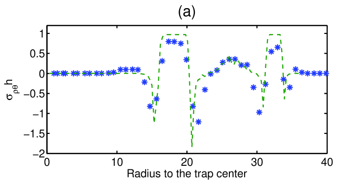
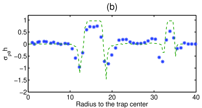
Figure 12: (Color online)   The effective local Hall conductance $\sigma_{\rho\theta}(r)$ v.s. $r$ defined in Eq. 44 at $\Omega/t_{\parallel}=\frac{3}{2}$ (a) and $2$ (b). The radius is in the unit of the lattice constant $a$. The results from diagonalizing the free Hamiltonian with the trapping potential is marked with asterisks, and those from the modified LDA are plotted with dashed lines.

In this subsection, we consider the large rotation angular velocities at $\Omega/t_{\parallel}=\frac{3}{2}$ and $2$ which are at and above $\Omega_{c}/t_{\parallel}=\frac{3}{2}$, respectively. The band structure topology above $\Omega_{c}$ changes to a different Chern number pattern of $C_{1}=-C_{2}=C_{3}=-C_{4}=1$. The chemical potential $\mu/t_{\parallel}$ is chosen to 3.5, which guarantees that all bands are filled at $r=0$.

The distributions of the filling number $\langle n(\vec{r})\rangle$ are depicted in Fig. 11 at (a) $\Omega/t_{\parallel}=\frac{3}{2}$ and (b) $\Omega/t_{\parallel}=2$, respectively. At $\Omega/t_{\parallel}=\frac{3}{2}$, the 2nd and 3rd bands touch each other at a Dirac cone located at the center of the BZ. The DOS vanishes linearly, and thus the density profile exhibits a soft slope instead of a flat plateau in Fig. 11 (a). In both Fig. 11 (a) and (b), the density distributions between the 1st and 2nd bands also exhibit soft slopes although there do exist a band gap in the homogeneous system. This is because the potential gradient increases as $r$ goes larger in the confining trap, which closes the small gap between the 1st and 2nd bands at large values of $\Omega$.

The local anomalous Hall conductances defined in Eq. 44 are depicted in Fig. 12 at $\Omega/t_{\parallel}=\frac{3}{2}$ and $2$. In the insulating plateaus between the 3rd and 4th bands, $\sigma_{\rho\theta}$ is close to the quantized value of $1/h$ for both rotation angular velocities. The small deviation comes from the finite width of the insulating regions. In the region with soft slopes of the distributions of $\langle n(r)\rangle$ between the 1st and 2nd bands, $\sigma_{\rho\theta}$ is significantly smaller than $1/h$ because this region is not rigorously insulating. In the inhomogeneous metallic regions, the values of the local anomalous Hall currents are non-quantized which are determined by the combined effects from the gradients of the trapping potential and the density distribution.

V.3 Temperature effects

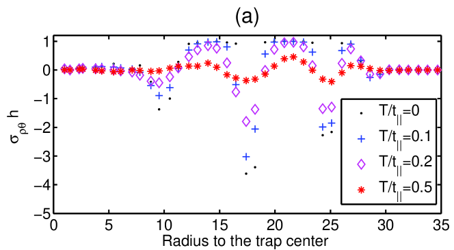
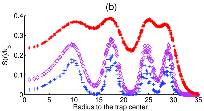
Figure 13: (Color online)   The radial distributions of (a) the anomalous Hall conductance $\sigma_{\rho\theta}(\vec{r},T)$ and (b) the entropy $S(\vec{r},T)$ with $\Omega/t_{\parallel}=\frac{3}{4}$. The black dot, blue “+”, magenta diamonds and red asterisks of the data represent temperatures at $T=0$, $T/t_{\parallel}=0.1$, $T/t_{\parallel}=0.2$ and $T/t_{\parallel}=0.5$, respectively.

In this subsection, we briefly discuss the finite temperature effects to the anomalous Hall conductance. The QAHE is a topological property existing in band insulating regions, thus it is robust against finite temperatures provided their scale is small compared to the band gap. On the other hand, we do expect that the anomalous Hall conductance in the metallic regions will be significantly affected by finite temperatures.

The radial distribution of the local anomalous Hall conductance $\sigma_{\rho\theta}^{\text{eff}}(r)$ v. s. $r$ is plotted in Fig. 13 (a) at different temperatures. The rotation angular velocity is taken as $\Omega/t_{\parallel}=\frac{3}{4}$. In this case, the band gaps are at the same order of $t_{\parallel}$ as shown in Fig. 7. $\sigma_{\rho\theta}$ remains nearly quantized in the insulating regions for $T/t_{\parallel}=0.1\sim 0.2$. According to the calculation of band structures in Ref. Wu and Das Sarma (2008), $t_{\parallel}\approx 0.24E_{r}$ at $V_{0}/E_{r}=15$ and the typical energy scale of $E_{r}$ is $0.1\sim 0.2\mu K$, thus the QAHE signature should survive at the order of $10$nK, which is an experimentally accessible temperature scale. In the metallic regions, naturally $\sigma_{\rho\theta}$’s are more strongly affected by finite temperatures. As $T$ further increases to the half value of $t_{\parallel}$, the quantized signatures of $\sigma_{\rho\theta}$ disappear.

We also present the entropy distributions in real space at various temperatures as shown in Fig. 13 (b). The local entropy is defined as

$$S(\vec{r},T) = -k_{B}\sum_{i}|\psi_{i}(\vec{r})|^{2}\Big{\{}n_{i}(T)\ln n_{i}(T)$$ (51)

$$+ (1-n_{i}(T))\ln[1-n_{i}(T)]\Big{\}},$$

where $k_{B}$ is the Boltzmann constant; the subscript $i$ is the index of energy levels; $\psi_{i}(\vec{r})$ is the wavefunction at the location $\vec{r}$; $n_{i}(T)$ is the Fermi distribution function. At low temperatures (e.g. $T/t_{\parallel}=0.1$ and $0.2$), $S(\vec{r},T)$ concentrates in the gapless metallic regions, and remains negligible in the band insulating regions. We have the coexistence of the insulating QAHE regions and the metallic regions to hold a significant amount of entropy. The tolerance of the large residue entropy densities in the trap greatly facilitates the experimental realization of the QAHE state. As temperatures go high, say, $T/t_{\parallel}=0.5$, the entropy distribution becomes more uniform, and there are no clear distinctions between insulating and metallic regions any more. This agrees with the picture in Fig. 13 (a), in which the plateaus of quantized anomalous Hall conductance disappear.

VI Experimental detections

In experiments, the plateaus of commensurate fillings of atoms in Fig. 8 and Fig. 11 can be observed by measuring the in-trap density distribution or the compressibility of the lattice system, as clearly demonstrated in recent experiments Jördens et al. (2008); Sherson et al. (2010); Schneider et al. (2008); Bakr et al. (2009). However, the density plateaus cannot distinguish the conventional band insulators and the quantum anomalous Hall insulators.

In solid state systems, the Hall conductivity are obtained from transport measurements, which are very difficult for the cold atom experiments. Nevertheless, it has been proposed to detect through the response of the atom density to an external magnetic field Umucalilar et al. (2008b), which can be realized by further rotating the harmonic trap Haljan et al. (2001) or coupling atoms with additional laser fields. In particular, the motion of atoms in laser fields leads to an artificial magnetic field, which has been observed in a recent experiment Lin et al. (2009). In the presence of an artificial magnetic field, the quantized anomalous Hall conductivity $\sigma_{xy}=\left(\frac{\partial n}{\partial B}\right)_{\mu}$, according to the well-known Streda formula Streda (1982) derived for the quantum Hall effects in the solid state. Therefore the density of atoms changes linearly with respect to the applied magnetic field when $\sigma_{xy}$ is quantized in some regions of the harmonic trap.

Another possible method to detect the anomalous Hall current is as follows. We assume all atoms are initially prepared in a hyperfine ground state $\left|1\right\rangle$. To detect the anomalous Hall current shown in Fig. 9, we apply a local two-photon Raman transition using two co-propagating focused laser beams in a small area $S$ to transfer atoms in $S$ to another hyperfine state $\left|2\right\rangle$. A subsequent time-of-flight measurement of the velocity distribution of atoms in state $\left|2\right\rangle$ gives the initial velocity distribution (thus the current) of atoms in the state $\left|1\right\rangle$ in the optical lattice. The above density and current measurements provide the experimental signature of the quantum anomalous Hall effects in the $p$-orbital honeycomb lattice.

VII Conclusions and Outlook

In summary, we have proposed the realization of the quantum anomalous Hall states in the cold atom optical lattices based on the experimentally available technique of the on-site rotation developed by Gemelke et al. This rotation generates the orbital Zeeman coupling whose energy scale can reach the order of the band width. In the $p$-orbital bands of the honeycomb lattice, the band structures become topologically non-trivial at any nonzero rotation angular velocities. A topological transition occurs at $\Omega_{c}/t_{\parallel}=\frac{3}{2}$ with different band Chern number patterns below and above $\Omega_{c}$. At $\Omega>\Omega_{c}$, the band topology is equivalent to a double copy of Haldane’s quantum anomalous Hall model. Flat band structures are also found at $\Omega/t_{\parallel}=\frac{3}{4}$ whose localized eigenstates can be constructed as circulating plaquette current states. The flat band structures may bring strong correlation effects, such as Wigner crystal and ferromagnetism, when interactions are turned on.

The effects of the spatial inhomogeneity to the $p$-orbital quantum anomalous Hall states are also investigated. At each commensurate filling of $\frac{1}{2},1,\frac{3}{2}$, and 2, the density profile exhibits insulating plateaus, whose Hall conductances are quantized at integer values. In the metallic regions between two adjacent plateaus, the anomalous Hall currents are determined by the non-local response, which can be understood as the combined effects of the gradients of the confining potential and particle density. We have also showed that the QAHE is robust at finite but low temperatures compared to band gaps.

We further point out that the generation of the quantum anomalous Hall states from this “orbital Zeeman” effect is very general, not just for the honeycomb lattice. The advantage of the $p$-orbital honeycomb lattice is that an infinitesimal value of $\Omega$ is enough to generate the quantum anomalous Hall states. For other generic lattice structures, beyond a critical value of $\Omega$ which is comparable to the band width, the orbital Zeeman effect generates inverted orbital bands of different orbital angular momenta. The further hybridization among them brings non-trivial band topology, which is a similar mechanism to achieve topological insulators in semi-conducting systems through spin-orbit couplings. A systematic study will be presented in a later publication.

References

- Gemelke et al. (2010) N. Gemelke, E. Sarajlic, and S. Chu, Rotating Few-body Atomic Systems in the Fractional Quantum Hall Regime, arXiv:1007.2677 (2010).
- Gemelke (2007) N. Gemelke, Ph.D. thesis (2007).
- Sarajic et al. (2009) E. Sarajic, N. Gemelke, S.-W. Chiow, S. Herrman, H. Müller, and S. Chu, Coherent control of ultracold matter: Fractional quantum hall physics and large-area atom interferometry (2009).
- Karplus and Luttinger (1954) R. Karplus and J. M. Luttinger, Phys. Rev. 95, 1154 (1954).
- Smit (1954) J. Smit, Physica 24, 39 (1954).
- Berger (1970) L. Berger, Phys. Rev. B 2, 4559 (1970).
- Jungwirth et al. (2002) T. Jungwirth, Q. Niu, and A. MacDonald, Phys. Rev. Lett. 88, 207208 (2002).
- Nagaosa (2006) N. Nagaosa, J. Phys. Soc. Jpn 75, 42001 (2006).
- Nagaosa et al. (2010) N. Nagaosa, J. Sinova, S. Onoda, A. H. MacDonald, and N. P. Ong, Reviews of Modern Physics 82, 1539 (2010).
- Xiao et al. (2009) D. Xiao, M.-C. Chang, and Q. Niu, arXiv:0907:2021 (2009).
- Qiao et al. (2010) Z. Qiao, S. A. Yang, W. Feng, W. Tse, J. Ding, Y. Yao, J. Wang, and Q. Niu, Chern Number Creation in Graphene from Rashba and Exchange Effects, arXiv:1005.1672 (2010).
- Tomizawa and Kontani (2009) T. Tomizawa and H. Kontani, Phys. Rev. B 80, 100401 (2009).
- Thouless et al. (1982) D. J. Thouless, M. Kohmoto, M. P. Nightingale, and M. den Nijs, Phys. Rev. Lett. 49, 405 (1982).
- Kohmoto (1985) M. Kohmoto, Ann. Phys. 160, 296 (1985).
- Jackiw (1984) R. Jackiw, Phys. Rev. D 29, 2375 (1984).
- Fradkin et al. (1986) E. Fradkin, E. Dagotto, and D. Boyanovsky, Phys. Rev. Lett. 57, 2967 (1986).
- Haldane (1988) F. D. M. Haldane, Phys. Rev. Lett. 61, 2015 (1988).
- Dyakonov and Perel (1971) M. I. Dyakonov and V. I. Perel, Physics Letters A 35, 459 (1971).
- Hirsch (1999) J. E. Hirsch, Phys. Rev. Lett. 83, 1834 (1999).
- Sinova et al. (2004) J. Sinova, D. Culcer, Q. Niu, N. A. Sinitsyn, T. Jungwirth, and A. H. MacDonald, Phys. Rev. Lett. 92, 126603 (2004).
- Murakami et al. (2003) S. Murakami, N. Nagaosa, and S.-C. Zhang, Science 301, 1348 (2003).
- Kato et al. (2004) Y. K. Kato, R. C. Myers, A. C. Gossard, and D. D. Awschalom, Science 306, 1910 (2004).
- Wunderlich et al. (2005) J. Wunderlich, B. Kaestner, J. Sinova, and T. Jungwirth, Phys. Rev. Lett. 94, 047204 (2005).
- Bernevig et al. (2006) B. A. Bernevig, T. L. Hughes, and S.-C. Zhang, Science 314, 1757 (2006).
- Qi et al. (2008) X.-L. Qi, T. L. Hughes, and S.-C. Zhang, Phys. Rev. B 78, 195424 (2008).
- Kane and Mele (2005) C. L. Kane and E. J. Mele, Phys. Rev. Lett. 95, 146802 (2005).
- Sheng et al. (2006) D. N. Sheng, Z. Y. Weng, L. Sheng, and F. D. M. Haldane, Phys. Rev. Lett. 97, 036808 (2006).
- Moore and Balents (2007) J. E. Moore and L. Balents, Phys. Rev. B 75, 121306 (2007).
- Roy (2009) R. Roy, Phys. Rev. B 79, 195321 (2009).
- Fu et al. (2007) L. Fu, C. L. Kane, and E. J. Mele, Phys. Rev. Lett. 98, 106803 (2007).
- Fu and Kane (2007) L. Fu and C. L. Kane, Phys. Rev. B 76, 045302 (2007).
- Zhang et al. (2009a) H. Zhang, C.-X. Liu, X.-L. Qi, X. Dai, Z. Fang, and S.-C. Zhang, Nat Phys 5, 438 (2009a).
- Wu et al. (2006) C. Wu, B. A. Bernevig, and S.-C. Zhang, Phys. Rev. Lett. 96, 106401 (2006).
- Xu and Moore (2006) C. Xu and J. E. Moore, Phys. Rev. B 73, 064417 (2006).
- König et al. (2007) M. König, S. Wiedmann, C. Brüne, A. Roth, H. Buhmann, L. W. Molenkamp, X. L. Qi, and S. C. Zhang, Science 318, 766 (2007).
- Hsieh et al. (2008) D. Hsieh, D. Qian, L. Wray, Y. Xia, Y. S. Hor, R. J. Cava, and M. Z. Hasan, Nature 452, 970 (2008).
- Hsieh et al. (2009) D. Hsieh, Y. Xia, L. Wray, D. Qian, A. Pal, J. H. Dil, J. Osterwalder, F. Meier, G. Bihlmayer, C. L. Kane, et al., Science 323, 919 (2009).
- Xia et al. (2009) Y. Xia, D. Qian, D. Hsieh, L. Wray, A. Pal, H. Lin, A. Bansil, D. Grauer, Y. S. Hor, R. J. Cava, et al., Nat Phys 5, 398 (2009).
- Chen et al. (2009) Y. L. Chen, J. G. Analytis, J.-H. Chu, Z. K. Liu, S.-K. Mo, X. L. Qi, H. J. Zhang, D. H. Lu, X. Dai, Z. Fang, et al., Science 325, 178 (2009).
- Roushan et al. (2009) P. Roushan, J. Seo, C. V. Parker, Y. S. Hor, D. Hsieh, D. Qian, A. Richardella, M. Z. Hasan, R. J. Cava, and A. Yazdani, Nature 460, 1106 (2009).
- Alpichshev et al. (2010) Z. Alpichshev, J. G. Analytis, J.-H. Chu, I. R. Fisher, Y. L. Chen, Z. X. Shen, A. Fang, and A. Kapitulnik, Phys. Rev. Lett. 104, 016401 (2010).
- Zhang et al. (2009b) T. Zhang, P. Cheng, X. Chen, J.-F. Jia, X. Ma, K. He, L. Wang, H. Zhang, X. Dai, Z. Fang, et al., Phys. Rev. Lett. 103, 266803 (2009b).
- Qi et al. (2006) X.-L. Qi, Y.-S. Wu, and S.-C. Zhang, Phys. Rev. B 74, 085308 (2006).
- Liu et al. (2008) C.-X. Liu, X.-L. Qi, X. Dai, Z. Fang, and S.-C. Zhang, Phys. Rev. Lett. 101, 146802 (2008).
- Onoda and Nagaosa (2003) M. Onoda and N. Nagaosa, Phys. Rev. Lett. 90, 206601 (2003).
- Yu et al. (2010) R. Yu, W. Zhang, H.-J. Zhang, S.-C. Zhang, X. Dai, and Z. Fang, Science 329, 61 (2010).
- Ho and Yip (2000) T. L. Ho and S. K. Yip, Phys. Rev. Lett. 84, 4031 (2000).
- Scarola and Sarma (2007) V. W. Scarola and S. D. Sarma, Phys. Rev. Lett. 98, 210403 (2007).
- Umucalilar et al. (2008a) R. O. Umucalilar, H. Zhai, and M. O. Oktel, Phys. Rev. Lett. 100, 070402 (2008a).
- Zhu et al. (2006) S.-L. Zhu, H. Fu, C. J. Wu, S. C. Zhang, and L. M. Duan, Phys. Rev. Lett. 97, 240401 (2006).
- Zhang (2010) C. Zhang, arXiv:1004.4231 (2010).
- Shao et al. (2008) L. B. Shao, S.-L. Zhu, L. Sheng, D. Y. Xing, and Z. D. Wang, Phys. Rev. Lett. 101, 246810 (2008).
- Stanescu et al. (2010) T. D. Stanescu, V. Galitski, and S. Das Sarma, Phys. Rev. A 82, 013608 (2010).
- Liu et al. (2010) X.-J. Liu, X. Liu, C. Wu, and J. Sinova, Phys. Rev. A 81, 033622 (2010).
- Goldman et al. (2010) N. Goldman, I. Satija, P. Nikolic, A. Bermudez, M. A. Martin-Delgado, M. Lewenstein, and I. B. Spielman, Phys. Rev. Lett. 105, 255302 (2010).
- Wu (2008a) C. Wu, Phys. Rev. Lett. 101, 186807 (2008a).
- Grynberg et al. (1993) G. Grynberg, B. Lounis, P. Verkerk, J. Y. Courtois, and C. Salomon, Phys. Rev. Lett. 70, 2249 (1993).
- Soltan-Panahi et al. (2010) P. Soltan-Panahi, J. Struck, P. Hauke, A. Bick, W. Plenkers, G. Meineke, C. Becker, P. Windpassinger, M. Lewenstein, and K. Sengstock, arXiv:1005.1276 (2010).
- Liu and Wu (2006) W. V. Liu and C. Wu, Phys. Rev. A 74, 013607 (2006).
- Stojanović et al. (2008) V. M. Stojanović, C. Wu, W. V. Liu, and S. Das Sarma, Phys. Rev. Lett. 101, 125301 (2008).
- Wu (2009) C. Wu, Modern Physics Letters B 23, 1 (2009).
- Isacsson and Girvin (2005) A. Isacsson and S. M. Girvin, Phys. Rev. A 72, 053604 (2005).
- Kuklov (2006) A. B. Kuklov, Phys. Rev. Lett. 97, 110405 (2006).
- Müller et al. (2007) T. Müller, S. Fölling, A. Widera, and I. Bloch, Phys. Rev. Lett. 99, 200405 (2007).
- Wirth et al. (2010) G. Wirth, M. Ölschläger, and A. Hemmerich, arXiv:1006.0509 (2010).
- Wu et al. (2007) C. Wu, D. Bergman, L. Balents, and S. Das Sarma, Phys. Rev. Lett. 99, 070401 (2007).
- Wu (2008b) C. Wu, Phys. Rev. Lett. 100, 200406 (2008b).
- Wu and Das Sarma (2008) C. Wu and S. Das Sarma, Phys. Rev. B 77, 235107 (2008).
- Zhang et al. (2010) S. Zhang, H.-h. Hung, and C. Wu, Phys. Rev. A 82, 053618 (2010).
- Lee et al. (2010) W.-C. Lee, C. Wu, and S. Das Sarma, Phys. Rev. A 82, 053611 (2010).
- Hung et al. (2009) H.-h. Hung, W.-C. Lee, and C. Wu, arXiv:0910.0507 (2009).
- Zhu et al. (2007) S.-L. Zhu, B. Wang, and L. M. Duan, Phys. Rev. Lett. 98, 260402 (2007).
- Lee et al. (2009) K. L. Lee, B. Grémaud, R. Han, B.-G. Englert, and C. Miniatura, Phys. Rev. A 80, 043411 (2009).
- Sun et al. (2010) K. Sun, Z. Gu, H. Katsura, and S. Das Sarma, ArXiv e-prints (2010), eprint 1012.5864.
- Neupert et al. (2010) T. Neupert, L. Santos, C. Chamon, and C. Mudry, ArXiv e-prints (2010), eprint 1012.4723.
- Tang et al. (2010) E. Tang, J. Mei, and X. Wen, ArXiv e-prints (2010), eprint 1012.2930.
- Leggett (2001) A. J. Leggett, Rev. Mod. Phys. 73, 307 (2001).
- Bak (1982) P. Bak, Rep. Prog. Phys. 45, 587 (1982).
- Bak (1986) P. Bak, Phys. Today 39, 38 (1986).
- Jördens et al. (2008) R. Jördens, N. Strohmaier, K. Günter, H. Moritz, and T. Esslinger, Nature 455, 204 (2008).
- Sherson et al. (2010) J. F. Sherson, C. Weitenberg, M. Endres, M. Cheneau, I. Bloch, and S. Kuhr, Nature 467, 68 (2010).
- Schneider et al. (2008) U. Schneider, L. Hackermuller, S. Will, T. Best, I. Bloch, T. A. Costi, R. W. Helmes, D. Rasch, and A. Rosch, Science 322, 1520 (2008).
- Bakr et al. (2009) W. S. Bakr, J. I. Gillen, A. Peng, S. Foelling, and M. Greiner, Nature 462, 74 (2009).
- Umucalilar et al. (2008b) R. O. Umucalilar, H. Zhai, and M. O. Oktel, Phys. rev. lett. 100, 070402 (2008b).
- Haljan et al. (2001) P. C. Haljan, I. Coddington, P. Engels, and E. A. Cornell, Phys. Rev. lett. 87, 210403 (2001).
- Lin et al. (2009) Y.-J. Lin, R. L. Compton, K. J. Garcia, J. V. Porto, and I. B. Spielman, Nature 462, 628 (2009).
- Streda (1982) P. Streda, J. Phys. C 15, L717 (1982).