Characterizing Galaxy Clusters with Gravitational Potential

Abstract

We propose a simple estimator for the gravitational potential of cluster-size halos using the temperature and density profiles of the intracluster gas based on the assumptions of hydrostatic equilibrium and spherical symmetry. Using high resolution cosmological simulations of galaxy clusters, we show that the scaling relation between this estimator and the gravitational potential has a small intrinsic scatter of $\sim 8\%-15\%$, and it is insensitive to baryon physics outside the cluster core. The slope and the normalization of the scaling relation vary weakly with redshift, and they are relatively independent of the choice of radial range used and the dynamical states of the clusters. The results presented here provide a possible way for using the cluster potential function as an alternative to the cluster mass function in constraining cosmology using galaxy clusters.

1. Introduction

Clusters of galaxies are useful probes of cosmology. The evolution of their abundance probes the growth of structure and therefore provides constraints on cosmological parameters (e.g., see Voit, 2005; Allen et al., 2011, for reviews). Clusters are readily observable in multiple wavelengths. In addition to the optical, the regime where galaxy clusters are first observed, hot gas in the deep gravitational wells of clusters shines in X-ray. In the sub-millimeter regime, galaxy clusters appear as distortions in the cosmic microwave background (CMB) as the hot electrons in the intracluster medium (ICM) scatter off CMB photons through inverse Compton scattering known as the Sunyaev–Zeldovich (SZ) effect (Sunyaev & Zeldovich, 1970; Carlstrom et al., 2002). In recent years, cosmological constraints have been yielded using cluster counts alone in optical surveys (e.g., Bahcall et al., 2003; Gladders et al., 2007; Rozo et al., 2010), in X-ray (e.g., Vikhlinin et al., 2009; Mantz et al., 2008, 2010), and in SZ (e.g., Vanderlinde et al., 2010; Sehgal et al., 2011). Cluster abundances and clustering also can also give us constraints on primordial non-gaussianity (e.g., Cunha et al., 2010) and models of gravity (e.g., Schmidt et al., 2009; Rapetti et al., 2010)

Ideally the simplest way to constrain cosmology is to measure the abundance of observable signals from clusters and constrain cosmology directly from them, e.g., constraining cosmology through direct comparison of the cluster temperature function predicted from theory against observations. However, current theoretical models are unable to model clusters by their observables to the precision necessary for constraining cosmological parameters down to percent level. On the other hand, theory does provide accurate and precise predictions of the cluster mass function (e.g., Jenkins et al., 2001; Warren et al., 2006; Tinker et al., 2008). The current paradigm of cluster cosmology therefore relies on estimating the cluster mass function from cluster observables via well-calibrated observable-mass relations.

Instead of focusing on cluster mass, an alternative is to characterize clusters by their gravitational potential, a quantity which is also well predicted by theory. Gravitational potential has potentially three advantages over mass. First, observable quantities, such as gas temperature and gravitational lensing signals, depend on the gravitational potential directly and only indirectly on mass. Therefore gravitational potential provides a more direct connection to cluster observables. Second, the shape of gravitational potential is more spherical than the matter distribution, and this may reduce the scatter in scaling relation due to the non-sphericity of matter distribution. Third, different definitions of halo mass exists, and they are not necessarily tied to the observable properties of cluster. For example, friends-of-friends (FoF) algorithm (e.g., Einasto et al., 1984; Davis et al., 1985), frequently used in defining halos in simulations, is difficult to implement in observations. Also, FoF halo in general has irregular shape (e.g., Lukić et al., 2009) and this poses another difficulty when relating to observations, where in most cases measurements are made within some circular annulus. Another way of defining a halo is through spherical overdensity, where average overdensity inside the halo is some value times the mean background density or the critical density of the universe. While this definition is more observationally-oriented, the halo mass defined this way artificially evolves with redshift as the mean background density and the critical density both change with redshift.

Efforts have been recently made both theoretically and observationally in characterizing clusters with their gravitational potential. Angrick & Bartelmann (2009) derived the abundance of cluster potential minima using a Gaussian random field formalism (Bardeen et al., 1986), and was used to predict cluster temperature function using a simple spherical-collapse model to model the nonlinear evolution of the cluster potential. On the observational side, Churazov et al. (2008, 2010) measured profiles of the gravitational potential of elliptical galaxies using both X-ray observations and stellar kinematics to constrain non-thermal pressure in those galaxies. It should then be straightforward, at least in principle, to extend these measurements to group and cluster-size systems.

In this paper, we show that the cluster potential can be measured reliably via observables, and that the cluster potential can serve as the defining quantity of cluster. We use simulations to estimate the gravitational potential of galaxy clusters by constructing a simple potential estimator based on intracluster gas profiles, motivated by the observational results of Churazov et al. (2008, 2010). In Section 2 we describe the simulations used in the paper. In Section 3 we describe our estimator of the cluster potential. In Section 4 we show the results of the scaling relations of this potential estimator and the gravitational potential. In Section 5 we give our summary and discussion.

2. Simulations

The simulation data we used are identical to those in Nagai et al. (2007a, b), where 16 cluster-sized systems are simulated using the Adaptive Refinement Tree $N$-body$+$gas-dynamics code (Kravtsov, 1999; Kravtsov et al., 2002), which is an Eulerian code that uses adaptive refinement in space and time, and non-adaptive refinement in mass (Klypin et al., 2001) to achieve the dynamic ranges to resolve the cores of halos formed in self-consistent cosmological simulations. The simulations assume a flat $\Lambda$CDM model: $\Omega_{\rm m}=1-\Omega_{\Lambda}=0.3$, $\Omega_{\rm b}=0.04286$, $h=0.7$ and $\sigma_{8}=0.9$, where the Hubble constant is defined as $100h{\ \rm km\ s^{-1}\ Mpc^{-1}}$, and $\sigma_{8}$ is the mass variance within spheres of radius $8\,h^{-1}$ Mpc. The simulations were run using a uniform $128^{3}$ grid with eight levels of mesh refinement. The box size for CL101–CL107 is $120\,h^{-1}$ Mpc comoving on a side and is $80\,h^{-1}$ Mpc comoving for CL3–CL24. This corresponds to peak spatial resolution of $\approx 7\,h^{-1}$ kpc and $5\,h^{-1}$ kpc for the two box sizes respectively. Only the inner regions $\sim 3$–$10\,h^{-1}$ Mpc surrounding the cluster center were adaptively refined. The dark matter (DM) particle mass in the region around each cluster was $m_{\rm p}\simeq 9.1\times 10^{8}\,h^{-1}\,{M_{\odot}}$ for CL101–107 and $m_{\rm p}\simeq 2.7\times 10^{8}\,h^{-1}\,{M_{\odot}}$ for CL3–24, while other regions were simulated with a bottom mass resolution.

In Table 1 we report $r_{500c}$ (the radius of the cluster within which its average density is 500 times the critical density), $M_{500c}$ (the mass within $r_{500c}$), and our classification of the dynamical state of the cluster based on the morphology of their mock X-ray images. Details of the classification can be found in Nagai et al. (2007b). The cluster center is defined as the location of the potential minimum.

We assess the effects of dissipative gas physics on the relation between the cluster potential and gas properties by comparing two sets of clusters simulated with the same initial conditions but with different prescription of gas physics. In the first set, the gas follows simple physics without any radiative cooling or star formation. We refer this set of clusters as non-radiative (NR) clusters. In the second set, metallicity-dependent radiative cooling, star formation, supernova feedback and a uniform UV background were added. We refer this set of clusters as cooling+star formation (CSF) clusters. For a detailed description of the gas physics implemented in the CSF clusters, please see Nagai et al. (2007a).

Table 1Properties of the Simulated Clusters at $z=0$

Cluster ID	$M_{500c}$	$r_{500c}$	Relaxed (1)
	(1014 $h^{-1}{M_{\odot}}$)	($h^{-1}$ Mpc)	/Unrelaxed (0)
CL101	9.02	1.16	0
CL102	5.45	0.98	0
CL103	5.70	0.99	0
CL104	5.40	0.98	1
CL105	4.86	0.94	0
CL106	3.47	0.84	0
CL107	2.57	0.76	1
CL3	2.09	0.71	1
CL5	1.31	0.61	1
CL6	1.68	0.66	0
CL7	1.42	0.63	1
CL9	0.83	0.52	0
CL10	0.67	0.49	1
CL11	0.90	0.54	0
CL14	0.77	0.51	1
CL24	0.35	0.39	0

3. Estimator of the Gravitational Potential

Following Churazov et al. (2008), we use a simple estimator of the cluster potential based on gas observables. Under the assumptions of hydrostatic equilibrium, the gradient of the gravitational potential is related to the pressure gradient and density of gas by

$$\nabla\phi=-\frac{\nabla P}{\rho_{g}},$$ (1)

where $\phi$ is the gravitational potential, $\rho_{g}$ is the density of the intracluster gas, and $P$ is the gas pressure. The gravitational potential can be obtained as a function of gas temperature $T$ and gas density when we integrate Equation (1) by parts:

$$\phi=-\int\frac{{d}P}{\rho_{g}}+{\rm constant}=-\frac{k_{\rm B}T}{\mu m_{\rm H}}-\int\frac{k_{\rm B}T}{\mu m_{\rm H}}{d}\ln\rho_{g}+{\rm constant}$$ (2)

where $k_{\rm B}$ is the Boltzmann constant, $\mu=0.59$ is the mean molecular weight for the fully ionized ICM, and $m_{\rm H}$ is the mass of the hydrogen atom.

Physical properties relate not to the absolute value of the potential but the difference in the potential. The difference of the spherically averaged gravitational potential between two arbitrary radii $r_{1}$ and $r_{2}$ can be directly calculated from the temperature and density profiles. We define our potential difference estimator which is based on the temperature and density profiles of the intracluster gas as $\Delta\psi$,

$$\Delta\psi\equiv\psi(r_{2})-\psi(r_{1})=-\left.\frac{kT(r)}{\mu m_{\rm H}}\right|^{2}_{1}-\int^{r_{2}}_{r_{1}}\frac{kT(r)}{\mu m_{\rm H}}\frac{{d}\ln\rho_{g}}{{d}r}{d}r\,.$$ (3)

One can note that $\psi$ is actually the enthalpy of the intracluster gas. If $\Delta\psi$ is a perfect estimator of the true potential difference $\Delta\phi$, then obviously we have $\Delta\psi=\Delta\phi$. Since in real clusters, neither the gravitational potential is strictly spherical, nor the intracluster gas obeys perfect hydrostatic equilibrium, we expect $\Delta\psi$ to deviate from $\Delta\phi$. To assess how well $\Delta\psi$ measures $\Delta\phi$ statistically, we fit a scaling relation of the two quantities using ordinary least squares:

$$\log\Delta\phi=\alpha\log\left(\Delta\psi/\Delta\psi_{0}\right)+\log\Delta\phi_{0}\,,$$ (4)

where we set $\mu m_{\rm H}\Delta\psi_{0}=20$ keV. Assuming that the residuals follow a log-normal distribution, we calculate the intrinsic scatter as the root mean square of the residuals $\delta_{\ln\Delta\phi}$ divided by $\sqrt{N-2}$ where $N$ is the total number of clusters:

$$\sigma_{\ln\Delta\psi}^{2}=\frac{1}{N-2}\sum_{i}^{N}\left(\ln\Delta\phi_{i}-\alpha\ln\left(\Delta\psi/\Delta\psi_{0}\right)-\ln\Delta\phi_{0}\right)^{2}.$$ (5)

Note that we follow the convention of using natural log for the log-normal scatter.

As $\Delta\psi$ and $\Delta\phi$ are dimensionally the same, we expect the slope of the scaling relation between them to be close to unity. We therefore also compute the scatter of the relation assuming unity slope, i.e., $\alpha=1$. In this case, we compute the intrinsic scatter as the root mean square of the residuals divided by $\sqrt{N-1}$ because of one less free parameter. We estimate the errors of the parameters $\alpha$, $\log\Delta\phi_{0}$ and $\sigma_{\ln\Delta\psi}$ by generating $10^{5}$ bootstrap samples.

We calculate the radial profiles for each cluster using logarithmically spaced bins, with a total of 100 bins spanning a comoving radial range from $1$ $h^{-1}$ kpc to $5$ $h^{-1}$ Mpc. Note that our results are not affected by the exact details of the binning scheme. The potential difference $\Delta\phi$ for each cluster is calculated from the potential profile directly measured from the simulation. The potential at each radial bin is calculated as the volume-average of the potential over all hydrodynamic cells inside the bin.

To calculate $\Delta\psi$, we measure the spherically averaged gas density profile and temperature profile for each simulated cluster. The temperature profile is measured as mass-weighted temperature $T_{{\rm mw}}$ which is the correct representation of the average specific gas thermal energy. For each radial shell, $T_{{\rm mw}}$ is calculated as

$$T_{{\rm mw}}=\frac{\sum_{i}\rho_{i}T_{i}\Delta V_{i}}{\sum_{i}\rho_{i}\Delta V_{i}},$$ (6)

where $\rho_{i}$, $T_{i}$, and $\Delta V_{i}$ are the gas density, gas temperature, and volume of the cell $i$ inside the radial shell and summed over all cells inside the radial bin.

Although mass-weighted temperature can in principle be measured by combining X-ray and SZ observations (e.g., Ameglio et al., 2007; Mroczkowski et al., 2007; Puchwein & Bartelmann, 2007), X-ray observations alone do not measure the mass-weighted temperature. To approximate the temperature measured from X-ray spectra, we calculate $\Delta\psi$ with the spectroscopic-like temperature $T_{{\rm sl}}$ (Mazzotta et al., 2004) which describes the temperature measured by Chandra and XMM-Newton well:

$$T_{{\rm sl}}=\frac{\sum_{i}\rho_{i}^{2}T_{i}^{-0.75}T_{i}\Delta V_{i}}{\sum_{i}\rho_{i}^{2}T_{i}^{-0.75}\Delta V_{i}}$$ (7)

This weighting scheme preferentially weighs more toward regions with high gas density and low temperature. In our calculation of the spectroscopic-like temperature, we exclude cells that have temperature less than $10^{6}$ K, which is well below the instrumental response of current X-ray instruments. We denote different $\Delta\psi$ and the fitting parameters that use the mass-weighted temperature and the spectroscopic-like temperature by subscripts “${{\rm mw}}$” and “${{\rm sl}}$”, respectively.

4. Testing the Estimator

Table 2Scaling Relation Parameters at $z=0.0$ for $r_{1}=(0.0,0.2,0.4)r_{500c}$ and $r_{2}=r_{500c}$

		$z=0.0$
$[r_{1}/r_{500c},r_{2}/r_{500c}]=$		$[0.0,1.0]$	$[0.2,1.0]$	$[0.4,1.0]$
$\alpha_{{\rm mw}}$	CSF	$0.896\pm 0.098$	$1.018\pm 0.046$	$1.056\pm 0.066$
	NR	$0.965\pm 0.030$	$0.970\pm 0.035$	$1.017\pm 0.048$
$\alpha_{{\rm sl}}$	CSF	$0.984\pm 0.059$	$1.010\pm 0.043$	$1.051\pm 0.121$
	NR	$0.951\pm 0.041$	$0.946\pm 0.054$	$0.993\pm 0.061$
$\log(\mu m_{\rm H}\Delta\phi_{0,{\rm mw}})$	CSF	$1.607\pm 0.022$	$1.334\pm 0.014$	$1.362\pm 0.033$
	NR	$1.327\pm 0.007$	$1.333\pm 0.014$	$1.356\pm 0.035$
$\log(\mu m_{\rm H}\Delta\phi_{0,{\rm sl}})$	CSF	$1.686\pm 0.013$	$1.375\pm 0.015$	$1.476\pm 0.067$
	NR	$1.336\pm 0.008$	$1.342\pm 0.019$	$1.370\pm 0.037$
$\sigma_{\ln\Delta\phi,{{\rm mw}}}$	CSF	$0.182\pm 0.027$	$0.088\pm 0.021$	$0.140\pm 0.035$
	NR	$0.064\pm 0.014$	$0.085\pm 0.019$	$0.131\pm 0.028$
$\sigma_{\ln\Delta\phi,{{\rm sl}}}$	CSF	$0.121\pm 0.017$	$0.072\pm 0.016$	$0.190\pm 0.024$
	NR	$0.075\pm 0.010$	$0.110\pm 0.016$	$0.147\pm 0.026$
		Fixed slope $\alpha=1$
		$z=0.0$
$[r_{1}/r_{500c},r_{2}/r_{500c}]=$		$[0.0,1.0]$	$[0.2,1.0]$	$[0.4,1.0]$
$\log(\mu m_{\rm H}\Delta\phi_{0,{\rm mw}})$	CSF	$1.597\pm 0.020$	$1.330\pm 0.009$	$1.335\pm 0.015$
	NR	$1.330\pm 0.007$	$1.341\pm 0.009$	$1.347\pm 0.014$
$\log(\mu m_{\rm H}\Delta\phi_{0,{\rm sl}})$	CSF	$1.686\pm 0.013$	$1.372\pm 0.008$	$1.419\pm 0.019$
	NR	$1.340\pm 0.008$	$1.360\pm 0.012$	$1.374\pm 0.015$
$\sigma_{\ln\Delta\phi,{{\rm mw}}}$	CSF	$0.195\pm 0.029$	$0.091\pm 0.023$	$0.148\pm 0.038$
	NR	$0.070\pm 0.015$	$0.090\pm 0.018$	$0.136\pm 0.029$
$\sigma_{\ln\Delta\phi,{{\rm sl}}}$	CSF	$0.125\pm 0.017$	$0.074\pm 0.017$	$0.198\pm 0.020$
	NR	$0.083\pm 0.013$	$0.119\pm 0.019$	$0.152\pm 0.026$

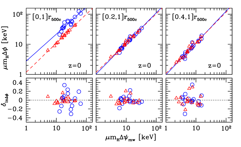
Figure 1.— Top panels: scaling relations of the potential difference $\Delta\phi$ and an estimator of the potential difference $\Delta\psi$ constructed from gas density and mass-weighted temperature. The potential and the gas observables are measured from three sets of radial separations: from the cluster center to $r_{500c}$ (left panel), from $0.2r_{500c}$ to $r_{500c}$ (middle panel), and from $0.4r_{500c}$ to $r_{500c}$ (right panel). The blue circles are for the CSF clusters and the red triangles are for the NR clusters. The blue solid line and the red dashed line are the fitted relation for the CSF and NR clusters respectively. The bottom panels show the corresponding residuals of the fits in the top panels.

We use high-resolution cosmological cluster simulations to compare the potential difference estimator $\Delta\psi$ with the real potential difference $\Delta\phi$ directly measured from the simulation. We have made following assumptions for our estimator.

1. Input gas physics has little or no effect on the robustness of the estimator.

2. The assumption of hydrostatic equilibrium is justified.

3. The use of spectroscopic-like temperature is adequate to estimate the potential with little increase in the scatter of the $\Delta\phi$–$\Delta\psi$ relation.

4. The $\Delta\phi$–$\Delta\psi$ relation does not evolve with redshift.

5. The intrinsic scatter of the $\Delta\phi$–$\Delta\psi$ relation follows log-normal distribution.

In the following, we test the validity of the assumptions (1) – (4) and quantify the amount of scatter in the $\Delta\phi$–$\Delta\psi$ relation. For (5), we need a larger sample of clusters to quantify the deviation from log-normal behavior for the scatter which we leave it for future work.

We report the values of the fitted slopes $\alpha$, normalization $\log(\mu m_{\rm H}\Delta\phi_{0})$ and intrinsic scatter $\sigma_{\ln\Delta\phi}$ of the $\Delta\phi$–$\Delta\psi$ scaling relations in upper halves of Table 2 – Table 4. In the lower halves of these tables, we report the normalization and intrinsic scatter where we fit the $\Delta\phi$–$\Delta\psi$ relation with the slope fixed to unity, $\alpha=1$. We report values of the fitted parameters estimated using both mass-weighted and spectroscopic-like temperatures wherever possible. Since we are measuring and estimating the potential difference between the inner radius $r_{1}$ and the outer radius $r_{2}$, for convenience we denote the radial interval for each scaling relation as $[r_{1},r_{2}]$.

Table 3Scaling Relation Parameters at $z=0.0,0.6,1.0$ for $r_{1}=0.2r_{500c}$ and $r_{2}=r_{500c}$

$[r_{1},r_{2}]=$		$[0.2r_{500c},r_{500c}]$
$z=$		$0.0$	$0.6$	$1.0$
$\alpha_{{\rm mw}}$	CSF	$1.018\pm 0.046$	$0.936\pm 0.050$	$0.912\pm 0.030$
	NR	$0.970\pm 0.035$	$0.901\pm 0.056$	$0.916\pm 0.054$
$\alpha_{{\rm sl}}$	CSF	$1.010\pm 0.043$	$0.852\pm 0.070$	$0.895\pm 0.034$
	NR	$0.946\pm 0.054$	$0.875\pm 0.062$	$0.881\pm 0.069$
$\log(\mu m_{\rm H}\Delta\phi_{0,{\rm mw}})$	CSF	$1.334\pm 0.014$	$1.324\pm 0.016$	$1.314\pm 0.018$
	NR	$1.333\pm 0.014$	$1.300\pm 0.025$	$1.321\pm 0.027$
$\log(\mu m_{\rm H}\Delta\phi_{0,{\rm sl}})$	CSF	$1.375\pm 0.015$	$1.350\pm 0.036$	$1.380\pm 0.023$
	NR	$1.342\pm 0.019$	$1.313\pm 0.030$	$1.332\pm 0.037$
$\sigma_{\ln\Delta\phi,{{\rm mw}}}$	CSF	$0.088\pm 0.021$	$0.094\pm 0.018$	$0.069\pm 0.011$
	NR	$0.085\pm 0.019$	$0.150\pm 0.022$	$0.080\pm 0.014$
$\sigma_{\ln\Delta\phi,{{\rm sl}}}$	CSF	$0.072\pm 0.016$	$0.150\pm 0.022$	$0.076\pm 0.013$
	NR	$0.110\pm 0.016$	$0.130\pm 0.014$	$0.107\pm 0.014$
		Fixed slope $\alpha=1$
$[r_{1},r_{2}]=$		$[0.2r_{500c},r_{500c}]$
$z=$		$0.0$	$0.6$	$1.0$
$\log(\mu m_{\rm H}\Delta\phi_{0,{\rm mw}})$	CSF	$1.330\pm 0.009$	$1.349\pm 0.010$	$1.353\pm 0.009$
	NR	$1.341\pm 0.009$	$1.345\pm 0.013$	$1.367\pm 0.010$
$\log(\mu m_{\rm H}\Delta\phi_{0,{\rm sl}})$	CSF	$1.372\pm 0.008$	$1.418\pm 0.017$	$1.436\pm 0.010$
$(\alpha=1)$	NR	$1.360\pm 0.012$	$1.372\pm 0.015$	$1.401\pm 0.014$
$\sigma_{\ln\Delta\phi,{{\rm mw}}}$	CSF	$0.091\pm 0.023$	$0.102\pm 0.021$	$0.087\pm 0.011$
	NR	$0.090\pm 0.018$	$0.129\pm 0.020$	$0.099\pm 0.026$
$\sigma_{\ln\Delta\phi,{{\rm sl}}}$	CSF	$0.074\pm 0.017$	$0.172\pm 0.024$	$0.099\pm 0.013$
	NR	$0.119\pm 0.019$	$0.153\pm 0.020$	$0.136\pm 0.035$

Table 4Scaling Relation Parameters at $z=0.0,0.6,1.0$ for $r_{1}=0.2r_{500c}$ and $r_{2}=r_{500c}$ for $\Delta\phi^{\rm NR}-\Delta\psi^{\rm CSF}$ Relation

$[r_{1},r_{2}]=$		$[0.2r_{500c},r_{500c}]$
$z=$		$0.0$	$0.6$	$1.0$
$\alpha_{{\rm mw}}$		$1.072\pm 0.088$	$1.002\pm 0.074$	$1.024\pm 0.068$
$\alpha_{{\rm sl}}$		$1.070\pm 0.084$	$0.867\pm 0.122$	$0.997\pm 0.086$
$\log(\mu m_{\rm H}\Delta\phi_{0,{\rm mw}})$		$1.271\pm 0.024$	$1.288\pm 0.022$	$1.278\pm 0.036$
$\log(\mu m_{\rm H}\Delta\phi_{0,{\rm sl}})$		$1.315\pm 0.026$	$1.295\pm 0.053$	$1.348\pm 0.050$
$\sigma_{\ln\Delta\phi,{{\rm mw}}}$		$0.184\pm 0.035$	$0.187\pm 0.045$	$0.137\pm 0.020$
$\sigma_{\ln\Delta\phi,{{\rm sl}}}$		$0.164\pm 0.031$	$0.270\pm 0.054$	$0.162\pm 0.030$
		Fixed slope $\alpha=1$
$[r_{1},r_{2}]=$		$[0.2r_{500c},r_{500c}]$
$z=$		$0.0$	$0.6$	$1.0$
$\log(\mu m_{\rm H}\Delta\phi_{0,{\rm mw}})$		$1.255\pm 0.019$	$1.287\pm 0.019$	$1.267\pm 0.014$
$\log(\mu m_{\rm H}\Delta\phi_{0,{\rm sl}})$		$1.297\pm 0.017$	$1.356\pm 0.028$	$1.350\pm 0.017$
$\sigma_{\ln\Delta\phi,{{\rm mw}}}$		$0.182\pm 0.036$	$0.180\pm 0.042$	$0.133\pm 0.029$
$\sigma_{\ln\Delta\phi,{{\rm sl}}}$		$0.163\pm 0.031$	$0.269\pm 0.058$	$0.157\pm 0.028$

4.1. Effects of Dissipation

Assuming hydrostatic equilibrium, we measure $\Delta\phi$ and $\Delta\psi_{{\rm mw}}$ in the simulated clusters for both CSF and NR clusters at $z=0$ for different radial distance separations: $[r_{1},r_{2}]$ where we set $r_{1}/r_{500c}=0,0.2$ and $0.4$, and fix $r_{2}=r_{500c}$, as it is the typical outermost radius current X-ray surveys are capable of measuring. This is also the radius within which the cluster is relaxed (Evrard et al., 1996) and where the non-thermal pressure small, $\lesssim 10\%$ (e.g., Evrard, 1990; Rasia et al., 2006; Nagai et al., 2007b). However, as we show later the estimator is robust to the exact choice of radial separation.

In Figure 1, we plot the $\Delta\phi$–$\Delta\psi_{{\rm mw}}$ relations for $[r_{1},r_{2}]/r_{500c}=[0,1],[0.2,1],[0.4,1]$ for both CSF and NR clusters. All slopes of the relations are within the expected value of unity to within $1\sigma$. The normalization $\log(\mu m_{\rm H}\Delta\psi_{0})$ is also near to the expected value of $\log 20\approx 1.3$. The intrinsic scatter varies from $\sim 6\%$ to $15\%$, depending on the radial separation and input cluster physics. In general the resulted scatters of the fixed slope relations increase slightly compared to those where the slope is a free parameter. The normalizations of the fixed slope relation remain unchanged to within $1\sigma$. The values of the fitted parameters are reported in Table 2.

For $[r_{1},r_{2}]/r_{500c}=[0.2,1],[0.4,1]$, the slope, normalization and scatter are similar for both CSF and NR clusters. Dissipative gas physics has little effect on the potential estimator outside the cluster core $r_{1}\gtrsim 0.2r_{500c}$.

For $[r_{1},r_{2}]/r_{500c}=[0,1]$, while the slope is similar in both CSF and NR clusters, the normalization of the CSF relation is offset to a higher value compared to the NR relation. As we discuss in Section 4.2, the higher normalization is due to strong gas rotation in the CSF clusters, where $\Delta\psi$ underestimates $\Delta\phi$, shifting the data points to the left in the $\Delta\phi$–$\Delta\psi_{{\rm mw}}$ plane. This underestimation is also shown in the upper left panel of Figure 3, where $\Delta\psi_{{\rm mw}}/\Delta\phi$ is plotted as a function of the inner radius $r_{1}$. The CSF relation have a relatively large scatter of about $18\%$ due to strong dissipation in the cluster core regions.

The potential estimator $\Delta\psi$ is robust to dissipational gas physics outside the cluster core. As we show in Section 4.2 that once we correct for non-thermal pressure support due the gas motions, the estimator becomes robust to gas physics even when the cluster core is included.

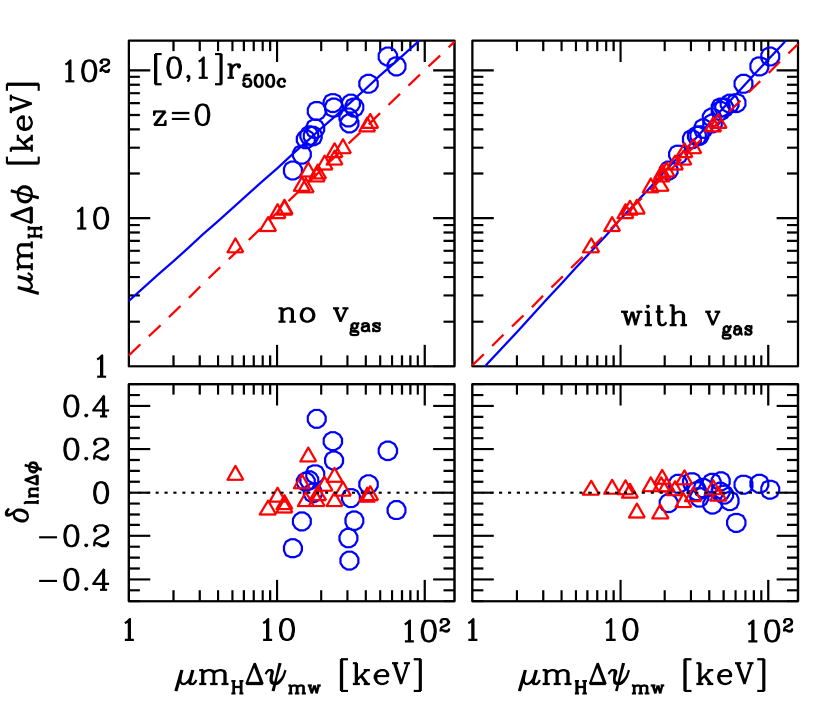
Figure 2.— Top panels: Scaling relations of the potential difference $\Delta\phi$ and an estimator of the potential difference $\Delta\psi$ constructed from gas density and mass-weighted temperature. The potential and the gas observables are measured from the cluster center to $r_{500c}$. The left panel shows the scaling relation without including pressure due to gas motions, while right panel shows the scaling relation with gas motions. The blue circles are for the CSF clusters and the red triangles are for the NR clusters. The blue solid line and the red dashed line are the fitted relation for the CSF and NR clusters respectively. The bottom panels show the corresponding residuals of the fits in the top panels.

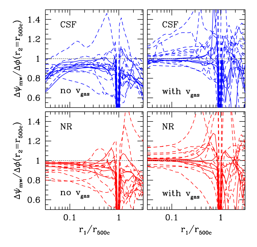
Figure 3.— $\Delta\psi_{{\rm mw}}/\Delta\phi$ as a function of the inner radius $r_{1}$ with the outer radius $r_{2}=r_{500c}$ at $z=0$. The solid lines represent relaxed clusters and the dashed lines represent unrelaxed clusters. Top panels show the CSF clusters and the bottom panels show the NR clusters. The left panels show the fiducial $\Delta\psi_{{\rm mw}}$ without including gas motions, while the right panels include pressure support form gas motions.

4.2. Non-thermal Pressure Support

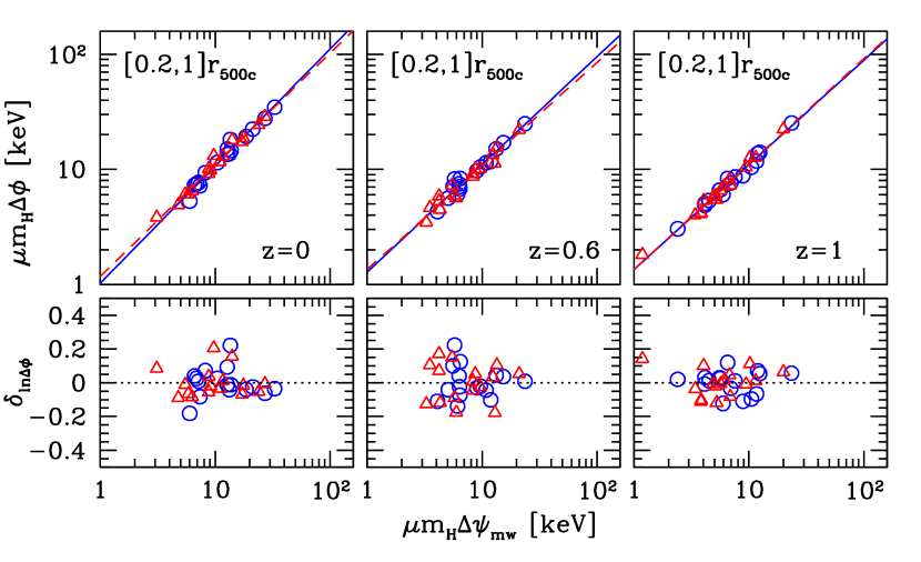
Figure 4.— Top panels: scaling relations of the potential difference $\Delta\phi$ and the potential difference estimator $\Delta\psi_{{\rm mw}}$ for a fixed radial separation with the inner radius $r_{1}=0.2r_{500c}$ and the outer radius $r_{2}=r_{500c}$ at different redshift: $z=0$ (left panel), $z=0.6$ (middle panel), and $z=1$ (right panel). The blue circles are for the CSF clusters and the red triangles are for the NR clusters. The blue solid line and the red dashed line are the fitted relation for the CSF and NR clusters respectively. The bottom panels show the corresponding residuals of the fits in the top panels.

We test the validity of the assumption of hydrostatic equilibrium of our potential estimator by explicitly including the contribution of non-thermal pressure support by gas motions, which are mainly responsible for the departure of hydrostatic equilibrium in our simulated clusters (Lau et al., 2009). The effects of gas motions can be corrected by including the following term $\Delta{\psi}_{\rm v_{gas}}$ in Equation (3), derived from the spherically symmetric radial Jean’s equation (e.g., Binney & Tremaine, 2008):

$$\Delta{\psi}_{\rm v_{gas}}=-\left(\overline{v_{r}^{2}}(r_{2})-\overline{v_{r}^{2}}(r_{1})\right)-\int^{r_{2}}_{r_{1}}\overline{v_{r}^{2}}\frac{{d}\ln\rho_{g}}{{d}r}{{d}r}-\int^{r_{2}}_{r_{1}}\frac{2\overline{v_{r}^{2}}-\overline{v_{t}^{2}}}{r}{{d}r}$$ (8)

where $\overline{v_{r}^{2}}$ and $\overline{v_{t}^{2}}$ are the radial and tangential components of the mean-square gas velocities averaged over the spherical radial shell, with respect to the cluster peculiar velocity defined as the average mass-weighted velocity of DM inside $r_{500c}$.

Figure 2 shows the scaling relation with and without the inclusion of the non-thermal pressure term $\Delta{\psi}_{\rm v_{gas}}$. Including gas motions, i.e., replacing $\Delta{\psi}_{{\rm mw}}$ with $\Delta{\psi}_{{\rm mw}}+\Delta{\psi}_{\rm v_{gas}}$, results in better estimates of the potential difference by decreasing the scatter of the scaling relation to $\sim 5\%$ for $[0,1]r_{500c}$ for both NR and CSF clusters This is illustrated more clearly in Figure 3 where we plot the deviations of the estimated potential difference $\Delta\psi_{{\rm mw}}$ from the true potential difference $\Delta\phi$ as a function of $r_{1}$ with $r_{2}$ fixed at $r_{500c}$, with solid lines representing the dynamically relaxed clusters and dashed lines representing the unrelaxed clusters. Without the inclusion of gas motions, $\Delta\psi_{{\rm mw}}$ underestimates $\Delta\phi$ by about $\sim 5\%$–$20\%$ for $r_{1}\gtrsim 0.1r_{500c}$ in both NR and CSF clusters, a value that is consistent with gas motions biasing the thermal pressure low by about the same amount (Lau et al., 2009). Most of the scatter is driven by the dynamically disturbed systems in the sample. For $r_{1}$ approaching $r_{2}=r_{500c}$, the scatter in both CSF and NR clusters increases as the outer regions of the cluster are less relaxed. In the inner region $r_{1}\lesssim 0.1r_{500c}$, the deviations from hydrostatic equilibrium are approximately constant for the NR clusters, but for CSF clusters, $\Delta\psi_{{\rm mw}}$ increasingly underestimates $\Delta\phi$ as $r_{1}$ decreases due to strong gas rotation near the core where the gas is rotationally supported induced by gas cooling (Lau et al., 2011). Including gas motions takes into the account the effective potential due to the rotation, leading to a better recovery of the true potential difference and agreement between the scaling relations of the CSF and the NR clusters. This is shown in the upper-right panel of Figure 2.

4.3. Spectroscopic-like Temperature

The spectroscopic-like temperature $T_{{\rm sl}}$ (Equation (7)) is generally less than the mass-weighted temperature $T_{{\rm mw}}$ (Equation (6)), as it weighs toward colder and denser gas. As shown in Table 2, for different $[r_{1},r_{500c}]$ the scatter in the $\Delta\phi$–$\Delta\psi_{{\rm sl}}$ relation is also larger than $\Delta\phi$–$\Delta\psi_{{\rm mw}}$ relation, as $\Delta\psi_{{\rm sl}}$ is biased towards the colder and denser gas, whose fractions and locations vary across different clusters. Nevertheless, the scatter is increased only by a few percent, with the exception for $[r_{1},r_{2}]=[0.4,1]r_{500c}$ where the large scatter is driven by a single cluster which has abnormally low $T_{{\rm sl}}$ due to a dense gas clump.

Comparing the $\Delta\phi$–$\Delta\psi_{{\rm sl}}$ relation between the CSF and NR clusters, we find that the normalization for the CSF relations are slightly higher than their NR counterparts at large $r_{1}$, because of the relatively larger number of cold dense clumps in the CSF clusters than in the NR clusters. Nevertheless their normalization agree to within 1$\sigma$.

To account for the limited angular resolution of X-ray observations, when we measure $T_{{\rm sl}}$, we average it over a radial window of $\Delta r=100$ kpc centered on the radius of interest. Varying the size of this window from $50$ kpc to $200$ kpc has little effect in changing the $\Delta\phi$–$\Delta\psi_{{\rm sl}}$ relations.

4.4. Evolution with Redshift

Next, we investigate the evolution of the $\Delta\phi$–$\Delta\psi$ relations by fixing $[r_{1},r_{2}]=[0.2,1]r_{500c}$ and fit the relations at $z=0.0,0.6$ and $1.0$. Figure 4 shows the resulting plots. All the relations at higher redshift are consistent with the $z=0$ results to within $2\sigma$. Scatter decreases slightly with increasing redshift and there is a weak trend of decreasing slope with redshift. The values of the parameters are shown in Table 3.

The apparent weak evolution in the $\Delta\phi$–$\Delta\psi$ relation can perhaps be explained by the lack of change in the gravitational potential over time once the DM halo has formed. For example, Li et al. (2007) demonstrated semi-analytically that the circular velocity at the virial radius of the halo remains relatively unchanged throughout much of its mass accretion history. Given that our sample size is quite small (16 clusters), the apparent redshift evolution could be driven by a few clusters. A complete understanding of the redshift evolution of the potential well and a full characterization of the redshift evolution of the $\Delta\phi$–$\Delta\psi$ relation will require tests using simulations with more clusters and redshift outputs than the current study.

4.5. Choice of Radial Separations

In principle $r_{1}$ and $r_{2}$ that define $\Delta\phi\equiv\phi(r_{2})-\phi(r_{1})$ and $\Delta\psi$ can be chosen arbitrary. In practice, the best choice of $[r_{1},r_{2}]$ would be the one that gives the lowest scatter. Once corrected for pressure from gas motions, the larger $|r_{1}-r_{2}|$ will result in less scatter, as the integral in $\Delta\psi$ (Equation (3)) encompasses larger radial range thus making the estimator more robust to small-scale variations in gas density and temperature. For example, setting $[r_{1},r_{2}]=[0.1,2]r_{500c}$ gives a scatter of about $\sim 6\%$, compared to $\sim 8\%$ for $[r_{1},r_{2}]=[0.1,1]r_{500c}$. Decreasing $r_{1}$ also gives smaller scatter as long as one stays away from the cluster core for the CSF clusters. For example,the scatter decreases from $\sim 14\%$ for $[r_{1},r_{2}]=[0.4,1]r_{500c}$ to $\sim 9\%$ for $[r_{1},r_{2}]=[0.2,1]r_{500c}$. For $r_{2}>r_{500c}$, the cluster gas deviates from hydrostatic equilibrium significantly with radius and $\Delta\psi$ underestimates the true potential difference $\Delta\phi$. However, this underestimation is small. As shown in Figure 5, the slope and normalization of the scaling relation are essentially the same as the radial interval changes from $[r_{1},r_{2}]=[0.5,1]r_{500c}$ to $[r_{1},r_{2}]=[0.1,2]r_{500c}$. The underestimation in the potential is significantly less than that of the hydrostatic mass estimate because $\Delta\psi$ encompasses a large region of the cluster interior where deviation from hydrostatic equilibrium is small, while the hydrostatic cluster mass measured at a particular radius is dependent on the local value of the pressure gradient.

Following similar logic, the choice of $r_{1}$ and $r_{2}$ should not be limited to functions of $r_{500c}$. Defining $r_{1}$ and $r_{2}$ through $r_{500c}$ can be undesirable as $r_{500c}$ depends on cosmology through the Hubble parameter $H(z)$. One choice of the radial interval, independent of the halo radius, is simply the physical distance separations. Figure 6 shows the scaling relations for $[r_{1},r_{2}]=[0.2,1]$Mpc at $z=0.0$, $0.6$ and $1.0$. For this radial separation the $\Delta\phi$–$\Delta\psi$ relation has a relatively small scatter of $\sim$ $8\%$–$9\%$ for the given redshifts. The values of slope and the normalization of the relations are similar to those with $r_{1}$ and $r_{2}$ being functions of $r_{500c}$ . The relation is the same for the different input gas physics. Redshift evolution of the relation is weak but requires more investigation as discussed in Section 4.4.

4.6. Calibration for $N$-body Simulations

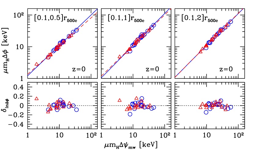
Figure 5.— Top panels: scaling relations of the potential difference $\Delta\phi$ and the potential difference estimator $\Delta\psi_{{\rm mw}}$ at $z=0$ for inner radius $r_{1}=0.1r_{500c}$ and outer radius $r_{2}=0.5r_{500c}$ (left panel), $r_{2}=r_{500c}$ (middle panel) and $r_{2}=2r_{500c}$ (right panel). The blue circles are for the CSF clusters and the red triangles are for the NR clusters. The blue solid line and the red dashed line are the fitted relation for the CSF and NR clusters respectively. The bottom panels show the corresponding residuals of the fits in the top panels.

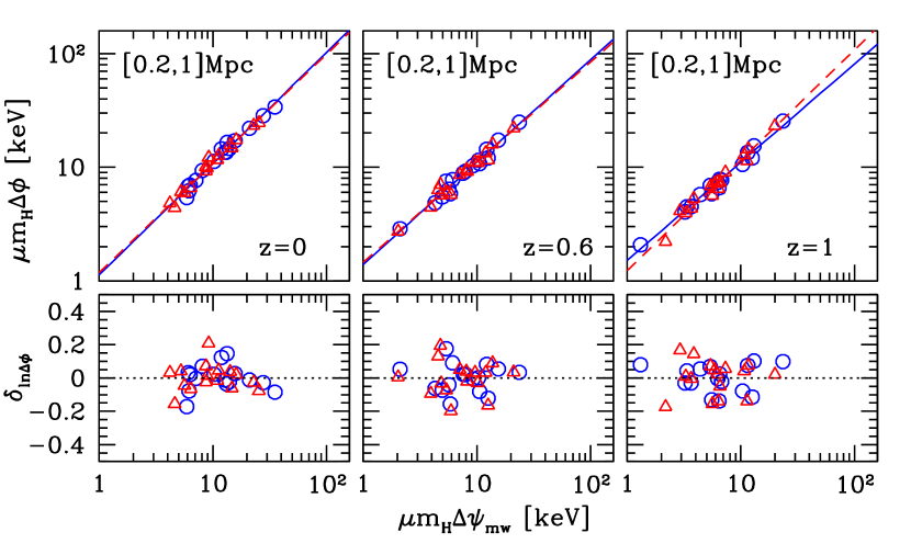
Figure 6.— Top panels: scaling relations of the potential difference $\Delta\phi$ and the potential difference estimator $\Delta\psi_{{\rm mw}}$ for a fixed radial separation with the inner radius $r_{1}=0.2$ Mpc and the outer radius $r_{2}=1$ Mpc at different redshift: $z=0$ (left panel), $z=0.6$ (middle panel), and $z=1$ (right panel). The blue circles are for the CSF clusters and the red triangles are for the NR clusters. The blue solid line and the red dashed line are the fitted relation for the CSF and NR clusters respectively. The bottom panels show the corresponding residuals of the fits in the top panels.

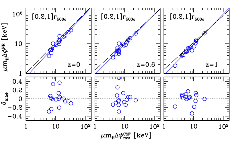
Figure 7.— Top panels: scaling relations of the potential difference $\Delta\phi^{\rm NR}$ in the NR clusters and the potential difference estimator $\Delta\psi_{{\rm mw}}^{\rm CSF}$ of the corresponding CSF clusters, for a fixed radial separation with the inner radius $r_{1}=0.2r_{500c}$ and the outer radius $r_{2}=0.5r_{500c}$ at different redshift: $z=0$ (left panel), $z=0.6$ (middle panel) and $z=1$ (right panel). The blue circles are for the CSF clusters and the red triangles are for the NR clusters. The blue solid line is fitted relation. The black dashed line is the best fit for the $\Delta\phi^{\rm CSF}$–$\Delta\psi_{{\rm mw}}^{\rm CSF}$ relation. The bottom panels show the corresponding residuals of the fits in the top panels.

Although becoming increasingly feasible, full cosmological hydrodynamical simulations of cluster formation with realistic physics like radiative cooling, star formation and active galactic nucleus feedback are expensive to run. A cheaper way would be using these simulations to calibrate less expensive dissipationless $N$-body simulations. Since both pure $N$-body simulations and our NR clusters have gravity as the only driving physics, the results of our NR clusters should be similar to the that of the $N$-body results. In this subsection, we therefore investigate how well our more realistic CSF clusters measure the gravitational potential wells of the NR clusters, and therefore the potential wells of clusters in $N$-body simulations. The results will be useful for calibrating a cluster potential function from pure $N$-body simulations.

We estimate the NR potential difference $\Delta\phi^{\rm NR}$ using the potential estimator of the CSF clusters $\Delta\psi^{\rm CSF}_{{\rm mw}}$. In Figure 7, we show the comparison between the $\Delta\phi^{\rm NR}$–$\Delta\psi^{\rm CSF}_{{\rm mw}}$ relation for $[r_{1},r_{2}]=[0.2,1]r_{500c}$ at $z=0.0,0.6$, and $1.0$ (in blue solid lines) and the $\Delta\phi^{\rm CSF}$–$\Delta\psi^{\rm CSF}_{{\rm mw}}$ relation (in black dashed lines). The slope of the $\Delta\phi^{\rm NR}$–$\Delta\psi^{\rm CSF}_{{\rm mw}}$ relation is steeper than the $\Delta\phi^{\rm CSF}$–$\Delta\psi^{\rm CSF}_{{\rm mw}}$ relation. This is because dissipation results in deeper potential wells in the CSF clusters compared to their NR counterparts, and this effect is stronger in small size halos which have lower virial temperature. Therefore $\Delta\psi^{\rm CSF}_{{\rm mw}}$ overestimates the potential difference $\Delta\phi^{\rm NR}$ more for the smaller size systems, leading to a steeper slope in the $\Delta\phi^{\rm NR}-\Delta\psi^{\rm CSF}_{{\rm mw}}$ relation. The scatter in $\Delta\phi^{\rm NR}$–$\Delta\psi^{\rm CSF}_{{\rm mw}}$ relation also increases because the NR clusters are not in exact identical dynamical states as their CSF counterparts as the dynamical evolution of each cluster halo is affected by the dissipative gas physics which changes the structure and hence dynamics of the halos. Table 4 summarizes the fitted parameters.

5. Summary and Discussion

5.1. Summary of Key Results

In this paper we propose a simple estimator for the gravitational potential difference in clusters of galaxies. This estimator is based on the density and temperature profiles of the intracluster gas under the assumptions of hydrostatic equilibrium and spherical symmetry.

Using high resolution cosmological hydrodynamical simulations of galaxy clusters, we have tested that this estimator is a robust and accurate estimator of the true gravitational potential of simulated clusters. The key results are summarized below:

1. The scaling relation between this estimator and the true gravitational potential difference $\Delta\phi$–$\Delta\psi$ has an intrinsic scatter of $\sim$ $8\%$–$15\%$.

2. Input gas physics has little effect on the $\Delta\phi$–$\Delta\psi$ relation as long as the cluster core is excised.

3. The assumption of hydrostatic equilibrium is justified outside the cluster core. Adding non-thermal pressure support reduces the scatter in the $\Delta\phi$–$\Delta\psi$ relation for all radii. The core need not be excised when non-thermal pressure support is included.

4. With the core excised or kinetic pressure from gas motions included, the slope and normalization of the $\Delta\phi$–$\Delta\psi$ scaling relation are relatively independent of the choice of radial separations. The scatter of the relation decreases as the separation increases.

5. The use of spectroscopic-like temperature is adequate to estimate the potential with little increase in scatter in the $\Delta\phi$–$\Delta\psi$ relation.

6. The $\Delta\phi$–$\Delta\psi$ relation evolves weakly with redshift. A full characterization of redshift evolution is needed.

The results presented above suggest that gravitational potential can serve as a useful alternative to cluster mass for cluster cosmology. X-ray mass-observable scaling relations are usually dependent on baryonic physics. For example, the normalization of the current tightest mass-observable relation, the $M$–$Y_{\rm X}$ relation (Kravtsov et al., 2006), is dependent on non-thermal pressure support; the normalization of the cluster mass–gas mass $M$–$M_{\rm gas}$ relation, is affected by the input gas physics (Fabjan et al., 2011). Our results show that the potential scaling relation, with appropriate radial range selection, is little affected by both of these effects.

Gravitational potential has another advantage over mass in that it is more spherical than that of the matter distribution. The assumption of spherical symmetry works better for gravitational potential than matter density, and this is perhaps partly why the potential scaling relation has relatively small scatter compared to mass-observable relations.

An essential characteristic of the gravitational potential scaling relation is that we are free to choose the radius where we measure the potential, not limiting to the halo radius defined in terms of overdensity with respect to the mean density of critical density of the universe, both of them functions of cosmology. This takes away the rather arbitrary nature of cluster mass, where different cluster mass definitions give different cluster mass functions (e.g., White, 2002; Tinker et al., 2008).

Despite the advantages given above, there are also several caveats and uncertainties in using the proposed potential estimator for cluster cosmology. We see a weakly evolving redshift evolution in the potential scaling relation that needs to be understood well before using gravitational potential for cluster cosmology. Although the potential measured at different radial separations result in essentially the same potential scaling relation, it is uncertain whether the different radial separation would result in different cluster potential function. Furthermore, we have assumed spherical symmetry for the gravitational potential and the gas distribution, but have not tested for the effect of deviation from spherical symmetry, although we expect that the effect to be small compared to the effect on cluster mass. Since our gravitational potential estimator involves an integral over radius of gas temperature and density, which is the dominant term in the estimator (Equation (3)), the gas density and temperature profiles may need to be measured with high spatial resolution. Accurate measurements of gas temperature also require high-resolution X-ray spectrometers. This can be technically challenging, especially if we want to measure the potential of high-$z$ clusters. However, we note that combined X-ray/SZ analysis is able to recover the temperature profile without the need of X-ray spectra (e.g., Nord et al., 2009).

5.2. Toward the Cluster Potential Function

Given the results presented in the paper, it will be interesting to see whether the cluster potential function is indeed a better alternative for constraining cosmology than the commonly adopted cluster mass function. In this subsection, we discuss ways to improve the potential scaling relations and to construct the cluster potential function.

We suggest that future modeling efforts toward the goal of using the cluster potential function for cluster cosmology should focus on two main areas: (1) further investigation on the intrinsic nature of the potential scaling relation and the properties of the cluster potential function and (2) implementation of the potential scaling relation in actual observations.

The first aspect aims to answer the question whether the cluster potential function can replace the cluster mass function for cosmology. To see whether the cluster potential function has more constraining power than the cluster mass function, comparison between the cluster potential function and the cluster mass function calibrated from the same large-scale simulation is required. The comparison will have to focus on whether cluster function recovers the fiducial cosmological parameters better in terms of degeneracies between parameters, statistical errors, and systematic uncertainties. Simulations with statistically large sample of clusters at multiple redshifts will help constraining the weak redshift evolution of the potential scaling relation shown in the current work. They will also help further characterize the scatter and systematics of the potential scaling relation, for example, deviations from lognormal distribution in the scatter.

The second aspect focuses on developing new ways of characterizing gravitational potentials based on cluster observables and apply them to synthetic and real observations. For example, the potential estimator proposed in the current work will benefit from mock X-ray analyses in addressing systematics like gas clumping (Mathiesen et al., 1999; Simionescu et al., 2011; Nagai & Lau, 2011) and some of its observational challenges discussed in the previous subsection. It is reasonable to expect that other types of cluster potential estimators exist and may even perform better than the one proposed in this paper. For example, gravitational lensing signals like shear and convergence depend on the projected gravitational potential and may provide a new probe to the gravitational potential. Velocity dispersion of cluster galaxies directly probes the cluster potential, although it can be affected by velocity anisotropy and projection effects. SZ signals measure the integrated gas pressure, and it is similar to the gas enthalpy-based estimator proposed in the current work. Multiple probes of the gravitational field will be helpful in determining systematics, and the covariance of different potential estimator may also improve the precision of the measured potential, as it is for the case of cluster mass proxies (Stanek et al., 2010).

Clearly, much more work is needed to address these issues and we hope that this paper provide a starting point for the investigation of using the cluster potential function for cosmology.

References

- Allen et al. (2011) Allen, S. W., Evrard, A. E., & Mantz, A. B. 2011, ARAA, in press, arXiv:1103.4829
- Ameglio et al. (2007) Ameglio, S., Borgani, S., Pierpaoli, E., & Dolag, K. 2007, MNRAS, 382, 397
- Angrick & Bartelmann (2009) Angrick, C., & Bartelmann, M. 2009, A&A, 494, 461
- Bahcall et al. (2003) Bahcall, N. A. et al. 2003, ApJ, 585, 182
- Bardeen et al. (1986) Bardeen, J. M., Bond, J. R., Kaiser, N., & Szalay, A. S. 1986, ApJ, 304, 15
- Binney & Tremaine (2008) Binney, J., & Tremaine, S. 2008, Galactic Dynamics (2nd ed.; Princeton Univ. Press)
- Carlstrom et al. (2002) Carlstrom, J. E., Holder, G. P., & Reese, E. D. 2002, ARA&A, 40, 643
- Churazov et al. (2008) Churazov, E., Forman, W., Vikhlinin, A., Tremaine, S., Gerhard, O., & Jones, C. 2008, MNRAS, 388, 1062
- Churazov et al. (2010) Churazov, E. et al. 2010, MNRAS, 404, 1165
- Cunha et al. (2010) Cunha, C., Huterer, D., & Doré, O. 2010, Phys. Rev. D, 82, 023004
- Davis et al. (1985) Davis, M., Efstathiou, G., Frenk, C. S., & White, S. D. M. 1985, ApJ, 292, 371
- Einasto et al. (1984) Einasto, J., Klypin, A. A., Saar, E., & Shandarin, S. F. 1984, MNRAS, 206, 529
- Evrard (1990) Evrard, A. E. 1990, ApJ, 363, 349
- Evrard et al. (1996) Evrard, A. E., Metzler, C. A., & Navarro, J. F. 1996, ApJ, 469, 494
- Fabjan et al. (2011) Fabjan, D., Borgani, S., Rasia, E., Bonafede, A., Dolag, K., Murante, G., & Tornatore, L. 2011, arXiv:1102.2903
- Gladders et al. (2007) Gladders, M. D., Yee, H. K. C., Majumdar, S., Barrientos, L. F., Hoekstra, H., Hall, P. B., & Infante, L. 2007, ApJ, 655, 128
- Jenkins et al. (2001) Jenkins, A., Frenk, C. S., White, S. D. M., Colberg, J. M., Cole, S., Evrard, A. E., Couchman, H. M. P., & Yoshida, N. 2001, MNRAS, 321, 372
- Klypin et al. (2001) Klypin, A., Kravtsov, A. V., Bullock, J. S., & Primack, J. R. 2001, ApJ, 554, 903
- Kravtsov (1999) Kravtsov, A. V. 1999, PhD thesis, New Mexico State Univ.
- Kravtsov et al. (2002) Kravtsov, A. V., Klypin, A., & Hoffman, Y. 2002, ApJ, 571, 563
- Kravtsov et al. (2006) Kravtsov, A. V., Vikhlinin, A., & Nagai, D. 2006, ApJ, 650, 128
- Lau et al. (2009) Lau, E. T., Kravtsov, A. V., & Nagai, D. 2009, ApJ, 705, 1129
- Lau et al. (2011) Lau, E. T., Nagai, D., Kravtsov, A. V., & Zentner, A. R. 2011, ApJ, 734, 93
- Li et al. (2007) Li, Y., Mo, H. J., van den Bosch, F. C., & Lin, W. P. 2007, MNRAS, 379, 689
- Lukić et al. (2009) Lukić, Z., Reed, D., Habib, S., & Heitmann, K. 2009, ApJ, 692, 217
- Mantz et al. (2008) Mantz, A., Allen, S. W., Ebeling, H., & Rapetti, D. 2008, MNRAS, 387, 1179
- Mantz et al. (2010) Mantz, A., Allen, S. W., Rapetti, D., & Ebeling, H. 2010, MNRAS, 406, 1759
- Mathiesen et al. (1999) Mathiesen, B., Evrard, A. E., & Mohr, J. J. 1999, ApJ, 520, L21
- Mazzotta et al. (2004) Mazzotta, P., Rasia, E., Moscardini, L., & Tormen, G. 2004, MNRAS, 354, 10
- Mroczkowski et al. (2007) Mroczkowski, T. et al. 2007, BAAS, 38, 857
- Nagai et al. (2007a) Nagai, D., Kravtsov, A. V., & Vikhlinin, A. 2007a, ApJ, 668, 1
- Nagai & Lau (2011) Nagai, D., & Lau, E. T. 2011, ApJ, 731, L10
- Nagai et al. (2007b) Nagai, D., Vikhlinin, A., & Kravtsov, A. V. 2007b, ApJ, 655, 98
- Nord et al. (2009) Nord, M. et al. 2009, A&A, 506, 623
- Puchwein & Bartelmann (2007) Puchwein, E., & Bartelmann, M. 2007, A&A, 474, 745
- Rapetti et al. (2010) Rapetti, D., Allen, S. W., Mantz, A., & Ebeling, H. 2010, MNRAS, 406, 1796
- Rasia et al. (2006) Rasia, E. et al. 2006, MNRAS, 369, 2013
- Rozo et al. (2010) Rozo, E. et al. 2010, ApJ, 708, 645
- Schmidt et al. (2009) Schmidt, F., Vikhlinin, A., & Hu, W. 2009, Phys. Rev. D, 80, 083505
- Sehgal et al. (2011) Sehgal, N. et al. 2011, ApJ, 732, 44
- Simionescu et al. (2011) Simionescu, A. et al. 2011, Science, 331, 1576
- Stanek et al. (2010) Stanek, R., Rasia, E., Evrard, A. E., Pearce, F., & Gazzola, L. 2010, ApJ, 715, 1508
- Sunyaev & Zeldovich (1970) Sunyaev, R. A., & Zeldovich, Y. B. 1970, Ap&SS, 7, 3
- Tinker et al. (2008) Tinker, J., Kravtsov, A. V., Klypin, A., Abazajian, K., Warren, M., Yepes, G., Gottlöber, S., & Holz, D. E. 2008, ApJ, 688, 709
- Vanderlinde et al. (2010) Vanderlinde, K. et al. 2010, ApJ, 722, 1180
- Vikhlinin et al. (2009) Vikhlinin, A. et al. 2009, ApJ, 692, 1060
- Voit (2005) Voit, G. M. 2005, Rev. Mod. Phys., 77, 207
- Warren et al. (2006) Warren, M. S., Abazajian, K., Holz, D. E., & Teodoro, L. 2006, ApJ, 646, 881
- White (2002) White, M. 2002, ApJS, 143, 241