KP line solitons and Tamari lattices

Abstract

The KP-II equation possesses a class of line soliton solutions which can be qualitatively described via a tropical approximation as a chain of rooted binary trees, except at “critical” events where a transition to a different rooted binary tree takes place. We prove that these correspond to maximal chains in Tamari lattices (which are poset structures on associahedra). We further derive results that allow to compute details of the evolution, including the critical events. Moreover, we present some insights into the structure of the more general line soliton solutions. All this yields a characterization of possible evolutions of line soliton patterns on a shallow fluid surface (provided that the KP-II approximation applies).

1 Introduction

The Kadomtsev-Petviashvili (KP) II equation possesses exact solutions consisting of an arbitrary number of line solitons [1, 2, 3, 4, 5]. More comprehensive studies of the structure of the rather complex networks emerging in this way have been undertaken quite recently [6, 7, 8, 9, 10, 11, 12, 13, 14, 15, 16, 17, 18] (see also the review [19] and the references cited therein). Whereas in these works a classification in terms of the asymptotic behavior at large negative and positive times, and large (positive or negative) values of the coordinate transverse to the main propagation direction, has been addressed, in the present work we proceed toward an understanding of the full evolution.

It is rather difficult to generate specific line soliton patterns in a laboratory (but see [18, 19] for recent progress). In order to test the validity of the KP approximation, there is at least the possibility to generate such networks by chance and then to observe their evolution qualitatively, i.e. as a (time-ordered) sequence of certain patterns. For a subclass of KP line soliton solutions we demonstrate in this work that the allowed evolutions are in correspondence with maximal chains in a Tamari lattice [20] (see also [21, 22, 23, 24, 25, 26, 27, 28, 29, 30, 31, 32, 33, 34, 35, 36] for some work related to Tamari lattices).

The Tamari lattice $\mathbb{T}_{n}$ can be defined as a partially ordered set (poset) in which the elements consist of different ways of grouping a sequence of $n+1$ objects into pairs using parentheses (binary bracketing). The partial order is imposed by allowing only a rightward application of the associativity law: $(ab)c\to a(bc)$. $\mathbb{T}_{1}$ has a single element, $(ab)$, which can also be represented as the rooted binary tree on the left side in Fig. 1. $\mathbb{T}_{2}$ is given by $(ab)c\to a(bc)$, which corresponds to the two rooted binary trees on the right of Fig. 1.

Figure 1: The tree on the left side represents the Tamari lattice $\mathbb{T}_{1}$ which consists of a single node. On the right side, a corresponding representation of $\mathbb{T}_{2}$ is shown.

For a sequence of four objects $abcd$, the five possible groupings are $((ab)c)d$, $(a(bc))d$, $a((bc)d)$, $a(b(cd))$ and $(ab)(cd)$. The Tamari lattice $\mathbb{T}_{3}$ then consists of the two chains $((ab)c)d\to(a(bc))d\to a((bc)d)\to a(b(cd))$ and $((ab)c)d\to(ab)(cd)\to a(b(cd))$, and thus forms a pentagon.

In section 2 we specify the class of KP line soliton solutions, which is the central object of this work, and demonstrate their rooted tree structure. In section 3 we make further steps toward a classification of such solutions as evolutions of rooted trees. This somewhat pedagogical approach is supplemented by general results derived in Appendix Appendix A: Some general results. Section 4 presents some insights concerning the understanding of general line soliton solutions. Section 5 draws some conclusions and briefly summarizes further results, elaborated in additional appendices.

2 Rooted tree structure of the simplest class of KP line soliton solutions

Writing the variable $u$ of the KP equation as

$$u=2\,\log(\tau)_{xx}\,,$$

with a function $\tau$, the KP equation

$$(-4\,u_{t}+u_{xxx}+6\,uu_{x})_{x}+3\,u_{yy}=0$$

(where e.g. $u_{x}=\partial u/\partial x$) is transformed into the Hirota bilinear form

$$4\,(\tau\,\tau_{xt}-\tau_{x}\,\tau_{t})-3\,(\tau\,\tau_{yy}-\tau_{y}{}^{2})-\tau\,\tau_{xxxx}+4\,\tau_{x}\,\tau_{xxx}-3\,\tau_{xx}{}^{2}=0\;.$$

The simplest class of line soliton solutions is then given by

$$\tau=\sum_{k=1}^{M+1}e^{\theta_{k}}\,,\qquad\theta_{k}=p_{k}\,x+p_{k}^{2}\,y+c_{k}\,,$$ (2.1)

provided we make the replacement

$$c_{k}\mapsto p_{k}^{3}\,t+c_{k}\;.$$ (2.2)

$p_{k},c_{k}$ are real constants and $M\in\mathbb{N}$. The absorption of the time variable $t$ into the parameter $c_{k}$ (via the inverse of the above redefinition) is very helpful at the moment. Without restriction of generality we can assume that $p_{1}<\cdots<p_{M+1}$. The $xy$-plane is divided into regions dominated by one of the phases (see also [8]). Let us call the region where $\theta_{i}>\theta_{k}$, for all $k\neq i$, the $\theta_{i}$-region. There we have

$$\log(\tau)=\theta_{i}+\log\Big{(}1+\sum_{j=1\atop j\neq i}^{M+1}e^{-(\theta_{i}-\theta_{j})}\Big{)}\simeq\theta_{i}\,,$$

where the approximation is valid sufficiently far away from the boundary. Hence

$$\log(\tau)\simeq\max\{\theta_{1},\ldots,\theta_{M+1}\}\,,$$

where the right hand side can be regarded as a tropical version of $\log(\tau)$ (see also Appendix Appendix D: Tropical approximation). Away from the boundary of a dominating phase region, $\max\{\theta_{1},\ldots,\theta_{M+1}\}$ is linear in $x$, hence $u$ vanishes. A line soliton branch thus corresponds to a boundary line between two dominating phase regions. This is the picture that underlies our approach toward a classification of KP line soliton solutions. For $M=1$ we have a single line soliton. Fig. 2 shows the case $M=2$.

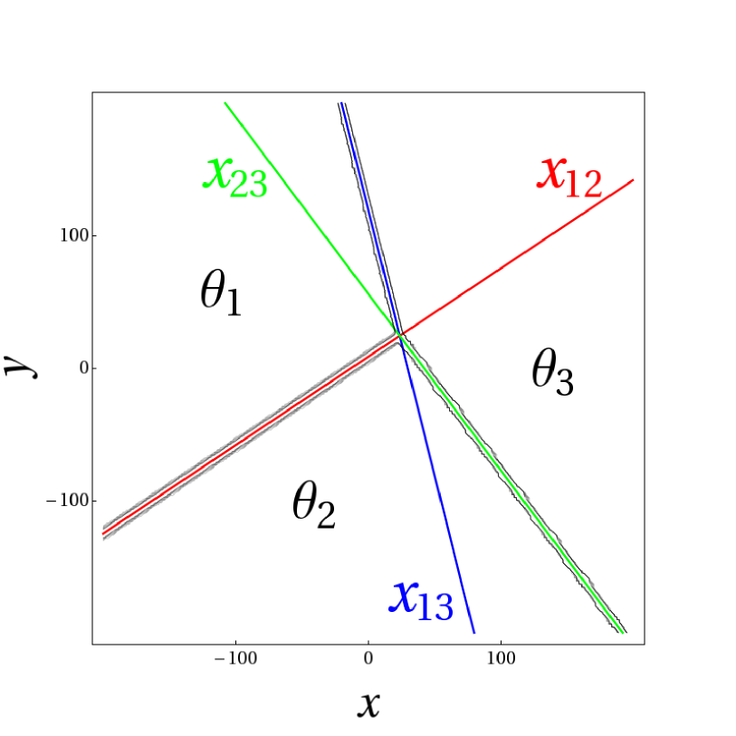
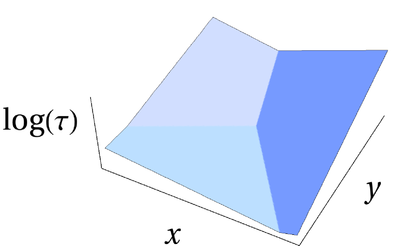
Figure 2: A contour plot of a line soliton solution with $M=2$ at a fixed time. This is an example of a “Miles resonance” [37]. The thin lines are boundary lines between two phase regions that are dominated by another phase, so that they are not visible in a line soliton plot. This solution keeps its form for all times (while moving from the right to the left) and can be represented by the trivial Tamari lattice $\mathbb{T}_{1}$. The right figure shows a plot of $\log(\tau)$ at the same time. It confirms the tropical description of the line soliton solution as the boundary between three planes determined by the tropical function $\max\{\theta_{1},\theta_{2},\theta_{3}\}$.

For $i\neq j$, we have

$$\theta_{i}-\theta_{j}=(p_{i}-p_{j})[x-x_{ij}(y)]\,,$$

where

$$x_{ij}(y)=-(p_{i}+p_{j})\,y-c_{ij}=x_{ji}(y)\,,\qquad c_{ij}=\frac{c_{i}-c_{j}}{p_{i}-p_{j}}=c_{ji}\;.$$

Hence $\theta_{i}=\theta_{j}$ determines the boundary line $x=x_{ij}(y)$ between the region where $\theta_{i}$ dominates $\theta_{j}$ and the region where $\theta_{j}$ dominates $\theta_{i}$. Such a line cannot be parallel to the $x$-axis. Consequently it divides the plane into a left and a right part.

Proposition 2.1.

For $p_{i}<p_{j}$ we have

$$\theta_{i}\,\gtrless\,\theta_{j}\qquad\mbox{for}\qquad x\lessgtr x_{ij}(y,t)\,,$$

i.e. $\theta_{i}$ dominates $\theta_{j}$ on the left side of the line $x=x_{ij}(y,t)$, and vice versa on the right side. $\square$

A particular consequence is that, for all $i=1,\ldots,M+1$, the $\theta_{i}$-region is convex, and thus in particular connected. For $M>1$ we have the identity

$$x_{ij}(y)-x_{ik}(y)=(p_{k}-p_{j})(y-y_{ijk})\qquad\mbox{with}\quad y_{ijk}=-c_{ijk}\,,$$ (2.3)

where

$$c_{ijk}=\frac{c_{ij}-c_{ik}}{p_{j}-p_{k}} = \frac{c_{i}}{(p_{i}-p_{j})(p_{i}-p_{k})}+\frac{c_{j}}{(p_{j}-p_{k})(p_{j}-p_{i})}+\frac{c_{k}}{(p_{k}-p_{i})(p_{k}-p_{j})}$$

$$= \frac{c_{i}}{(p_{i}-p_{j})(p_{i}-p_{j})}+\mbox{cyclic permutations}$$

is totally symmetric (i.e. invariant under arbitrary permutations of $i,j,k$). It follows that the boundary lines $(x_{ij}(y),y)$ and $(x_{ik}(y),y)$ meet in the point

$$P_{ijk}=(x_{ijk},y_{ijk})\,,$$

where

$$x_{ijk}=x_{ij}(y_{ijk})=-\frac{c_{i}(p_{j}^{2}-p_{k}^{2})+c_{j}(p_{k}^{2}-p_{i}^{2})+c_{k}(p_{i}^{2}-p_{j}^{2})}{(p_{i}-p_{j})(p_{j}-p_{k})(p_{k}-p_{i})}\;.$$

It further follows that also the line $(x_{jk}(y),y)$ passes through $P_{ijk}$. At the “critical point” $P_{ijk}$ we have $\theta_{i}=\theta_{j}=\theta_{k}$ (see also Fig. 2).

Proposition 2.2.

Let $p_{i}<p_{j}<p_{k}$. Then

$$\begin{array}[]{l}x_{ij}(y)<x_{ik}(y)<x_{jk}(y)\\ x_{ij}(y)>x_{ik}(y)>x_{jk}(y)\end{array}\quad\mbox{for}\quad\begin{array}[]{l}y<y_{ijk}\\ y>y_{ijk}\end{array}\;.$$

Proof: This is an immediate consequence of (2.3). $\square$

A (part of a) boundary line $x=x_{ij}(y)$ is called non-visible if it lies in a region where $\theta_{i}$ (or $\theta_{j}$) is dominated by another phase. Otherwise it is called visible. Correspondingly, the critical points can be classified as visible or non-visible. Visibility of $P_{ijk}$ means that at this point the $\theta_{i}$-, $\theta_{j}$-, and $\theta_{k}$-region meet.

Proposition 2.3.

Let $p_{i}<p_{j}<p_{k}$. Then the half-lines $\{x=x_{ij}(y)\,|\,y>y_{ijk}\}$, $\{x=x_{jk}(y)\,|\,y>y_{ijk}\}$ and $\{x=x_{ik}(y)\,|\,y<y_{ijk}\}$ are non-visible.

Proof: The following identity is easily verified,

$$\theta_{k}-\theta_{i}=(p_{k}-p_{i})[x-x_{ij}(y)+(p_{k}-p_{j})(y-y_{ijk})]\;.$$

Hence, along $x=x_{ij}(y)$, $y>y_{ijk}$, $\theta_{k}$ dominates $\theta_{i}$, so that this half-line is non-visible. The same identity written in the form

$$\theta_{i}-\theta_{k}=-(p_{k}-p_{i})[x-x_{jk}(y)-(p_{j}-p_{i})(y-y_{ijk})]\,,$$

respectively

$$\theta_{j}-\theta_{i}=(p_{j}-p_{i})[x-x_{ik}(y)-(p_{k}-p_{j})(y-y_{ijk})]\,,$$

implies the non-visibility of the other two half-lines. $\square$

As a consequence of the last proposition, if $P_{ijk}$ is visible, then only the half-lines $\{x=x_{ij}(y)\,|\,y<y_{ijk}\}$, $\{x=x_{jk}(y)\,|\,y<y_{ijk}\}$ and $\{x=x_{ik}(y)\,|\,y>y_{ijk}\}$ are visible in a neighborhood of $P_{ijk}$ (Fig. 2 shows the case $M=2$). Fig. 3 summarizes the process connected with the passage of $y$ through a critical value, corresponding to a visible critical point. This gives a rule to construct a poset for each $M>1$. The nodes are the phases and an edge is directed from $\theta_{i}$ to $\theta_{j}$ if $i<j$, assuming that $p_{1}<\cdots<p_{M+1}$. We assign $x_{ij}$ to the corresponding edge. For $M=2$ this yields a poset structure on a triangle, for $M=3$ on a tetrahedron (see Fig. 3), and more generally on the complete graph on $M+1$ nodes, which can be viewed as an $M$-simplex.

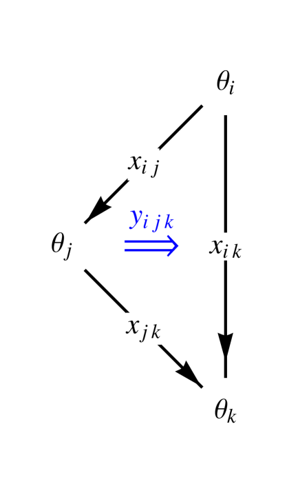
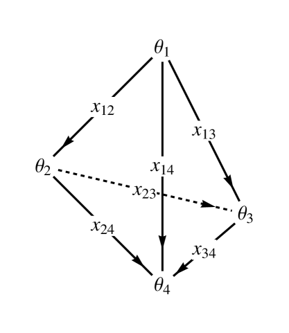
Figure 3: The left figure expresses what happens when $y$ passes a critical value $y_{ijk}$ corresponding to a visible critical point $P_{ijk}$ with $p_{i}<p_{j}<p_{k}$. The nodes coincide if $y=y_{ijk}$. For $y<y_{ijk}$ (left side of the left figure), $x_{ij}$ and $x_{ik}$ are visible (but not $x_{ik}$) and their order $x_{ij}<x_{ik}$ is expressed by the direction of the edges. For $y>y_{ijk}$ (vertical chain in the left figure), $x_{ik}$ is visible, but not the other two. The right figure shows the tetrahedron poset obtained in this way for $M=3$ with $p_{1}<p_{2}<p_{3}<p_{4}$. With each of its faces a critical value of $y$ is associated (and a corresponding “higher order” arrow), as in the left figure. Hence, e.g. for $y<\min\{y_{ijk}\}$ we have the chain $x_{12}<x_{23}<x_{34}$.

Proposition 2.4.

Let $p_{1}<p_{2}<\cdots<p_{M+1}$.
(1) For $y>\max\{y_{ijk}\}$, only the half-line $x=x_{1,M+1}(y)$ is visible.
(2) For $y<\min\{y_{ijk}\}$, all the half-lines $x=x_{m,m+1}(y)$, $m=1,\ldots,M$, are visible, and no other.

Proof: The following is a special case of the identity already used in the proof of Proposition 2.3,

$$\theta_{1}-\theta_{n}=(p_{1}-p_{n})[x-x_{1,M+1}(y)-(p_{M+1}-p_{n})(y-y_{1,n,M+1})]\;.$$

This implies $\theta_{1}>\theta_{n}$ along $x=x_{1,M+1}(y)$, $y>\max\{y_{ijk}\}$, for $n=2,\ldots,M$. Hence $x=x_{1,M+1}(y)$ is visible for large enough $y$. According to Proposition 2.3, all other lines are non-visible for large enough $y$. This proves (1). We also have

$$\theta_{m}-\theta_{n}=(p_{m}-p_{n})[x-x_{m,m+1}(y)-(p_{m+1}-p_{n})(y-y_{m,m+1,n})]\;.$$

Along $x=x_{m,m+1}(y)$, $y<\min\{y_{ijk}\}$, it implies $\theta_{m}>\theta_{n}$ for all $n\neq m,m+1$. As a consequence, this line is visible for large enough negative $y$, and this holds for $m=1,\ldots,M$. Again, Proposition 2.3 forbids other lines to be visible for large enough negative $y$, and this proves (2). $\square$

The last result (see also [13, 19]) implies the following asymptotic structure of a line soliton graph (from the restricted class considered in this section), see Fig. 4. For large enough $y$ there is only a single half-line. For large enough negative $y$ one observes $M$ lines. In particular, all $M+1$ regions of dominating phase extend to infinity in negative $y$-direction. This in turn implies that no bounded dominating phase regions exist (since the dominating phase regions are connected). Hence the graph has the structure of a rooted tree.

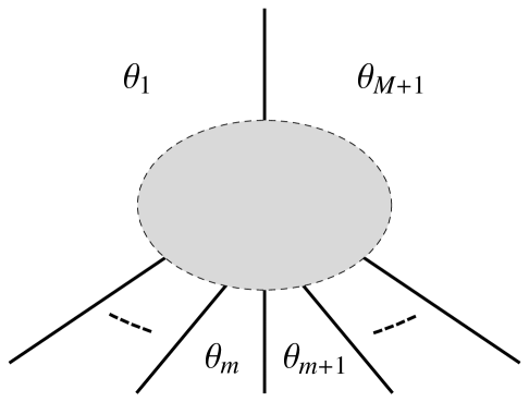
Figure 4: The asymptotic structure of a line soliton graph with $p_{1}<p_{2}<\cdots<p_{M+1}$. The order of the dominating phase regions is a consequence of $x_{m,m+1}<x_{m+1,m+2}$, $m=1,\ldots,M-1$, for $y$ smaller than all of its critical values, according to Proposition 2.2.

3 Time evolution of line soliton patterns

3.1 The first step

Let us reintroduce the time variable $t$ (which we hid away in the preceding section) via the replacement (2.2). Then we have

$$x_{ij}(y,t) = -(p_{i}+p_{j})\,y-(p_{i}^{2}+p_{i}p_{j}+p_{j}^{2})\,t-c_{ij}\,,$$

$$y_{ijk}(t) = -(p_{i}+p_{j}+p_{k})\,t-c_{ijk}\,,\qquad x_{ijk}(t)=x_{ij}(y_{ijk}(t),t)\,,$$

where $c_{ij}$ and $c_{ijk}$ are given by the previous formulae. The critical points $P_{ijk}$ now depend on $t$, hence they constitute “critical lines” in $\mathbb{R}^{3}$ (with coordinates $x,y,t$). For $M>2$ we have the identity

$$y_{ijk}(t)-y_{ijl}(t)=(p_{l}-p_{k})(t-t_{ijkl})\qquad\mbox{with}\quad t_{ijkl}=-c_{ijkl}\,,$$ (3.1)

where

$$c_{ijkl}=\frac{c_{ijk}-c_{ijl}}{p_{k}-p_{l}} = \frac{c_{i}}{(p_{i}-p_{j})(p_{i}-p_{k})(p_{i}-p_{l})}+\frac{c_{j}}{(p_{j}-p_{i})(p_{j}-p_{k})(p_{j}-p_{l})}$$

$$+\frac{c_{k}}{(p_{k}-p_{i})(p_{k}-p_{j})(p_{k}-p_{l})}+\frac{c_{l}}{(p_{l}-p_{i})(p_{l}-p_{j})(p_{l}-p_{k})}$$

$$= \frac{c_{i}}{(p_{i}-p_{j})(p_{i}-p_{k})(p_{i}-p_{l})}+\mbox{cyclic permutations}$$

is totally symmetric in the indices $i,j,k,l$. It follows that two critical points $P_{ijk}(t)$ and $P_{ijl}(t)$ coincide (only) at the time given by $t_{ijkl}$. Furthermore, at this value of time it turns out that also $P_{ikl}$ and $P_{jkl}$ coincide with this point. Hence we actually have a coincidence of (at least) four critical points. At the “critical event”

$$(P_{ijkl},t_{ijkl})\in\mathbb{R}^{3}\qquad\mbox{with}\qquad P_{ijkl}:=P_{ijk}(t_{ijkl})\,,$$

where the four critical lines intersect, we have $\theta_{i}=\theta_{j}=\theta_{k}=\theta_{l}$. For $M=3$, there is only a single critical time, namely $t_{1234}$, and $P_{1234}$ is visible at $t=t_{1234}$, i.e. a meeting point of line soliton branches (see Fig. 5). For $M>3$, there are ${M+1\choose 4}$ critical times, and the situation is more involved.

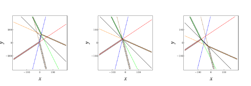
Figure 5: Evolution of a line soliton structure with $M=3$. These are snapshots at times $t<t_{1234}$ (left), $t=t_{1234}$ (middle) and $t>t_{1234}$ (right). Again, thin lines are boundary lines between two phase regions that are dominated by another phase and hence not visible in a line soliton plot. Disregarding the degenerate configuration at $t=t_{1234}$, this evolution can obviously be represented by the single chain of which the Tamari lattice $\mathbb{T}_{2}$ consists (see Fig. 1).

Proposition 3.1.

Let $p_{i}<p_{j}<p_{k}<p_{l}$. Then

$$\begin{array}[]{l}y_{ijk}(t)<y_{ijl}(t)<y_{ikl}(t)<y_{jkl}(t)\\ y_{ijk}(t)>y_{ijl}(t)>y_{ikl}(t)>y_{jkl}(t)\end{array}\quad\mbox{for}\quad\begin{array}[]{l}t<t_{ijkl}\\ t>t_{ijkl}\end{array}\;.$$

Proof: This is an immediate consequence of the identity (3.1). $\square$

Proposition 3.2.

Let $p_{i}<p_{j}<p_{k}<p_{l}$. Then
(1) $P_{ijl}(t)$ and $P_{jkl}(t)$ are non-visible for $t<t_{ijkl}$.
(2) $P_{ijk}(t)$ and $P_{ikl}(t)$ are non-visible for $t>t_{ijkl}$.

Proof: An identity used in the proofs of some propositions in section 2 generalizes via (2.2) to

$$\theta_{i}-\theta_{k}=(p_{i}-p_{k})[x-x_{ij}(y,t)+(p_{k}-p_{j})(y-y_{ijl}(t))+(p_{k}-p_{j})(p_{k}-p_{l})(t-t_{ijkl})]\;.$$

Evaluating this at $P_{ijl}(t)$, we obtain

$$\theta_{i}-\theta_{k}=(p_{k}-p_{i})(p_{k}-p_{j})(p_{l}-p_{k})(t-t_{ijkl})\,,$$

which is negative if $t<t_{ijkl}$, hence $P_{ijl}(t)$ is then non-visible. A similar argument applies in the other cases. $\square$

Proposition 3.3.

(1) For $t<\min\{t_{ijkl}\}$ only the critical points $P_{1,m,m+1}(t)$, $m=2,\ldots,M$, are visible.
(2) For $t>\max\{t_{ijkl}\}$ only the critical points $P_{m-1,m,M+1}(t)$, $m=2,\ldots,M$, are visible.

Proof: At $P_{1,m,m+1}(t)$ we have

$$\theta_{1}-\theta_{n}=-(p_{n}-p_{1})(p_{n}-p_{m})(p_{n}-p_{m+1})(t-t_{1,m,m+1,n})\,,$$

which, for $t$ smaller than all of its critical values, is positive for all $n$ different from $1,m,m+1$. Proposition 3.2, part 1, tells us that all other critical points are non-visible.

At $P_{m-1,m,M+1}(t)$ we have

$$\theta_{M+1}-\theta_{n}=(p_{M+1}-p_{n})(p_{n}-p_{m})(p_{n}-p_{m-1})(t-t_{n,m-1,m,M+1})\,,$$

which, for $t$ greater than all of its critical values, is positive for all $n$ different from $m-1,m,M+1$. Proposition 3.2, part 2, shows that all other critical points are non-visible. $\square$

Collecting our results, for $t$ smaller than all of its critical values the line soliton pattern can be represented by the left graph in Fig. 6 (note that $y_{1,m,m+1}<y_{1,m+1,m+2}$, $m=2,\ldots,M-1$, according to Proposition 3.1), and for $t$ greater than all of its critical values by the right graph (since then $y_{m,m+1,M+1}>y_{m+1,m+2,M+1}$, $m=1,\ldots,M-2$).

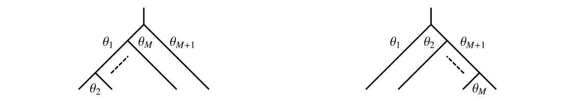
Figure 6: The structure of the solution for $t<\min\{t_{ijkl}\}$ (left tree) and $t>\max\{t_{ijkl}\}$ (right tree). For fixed $M$ these two trees form the maximal and the minimal element, respectively, of a Tamari lattice.

Together with Proposition 3.2, the next proposition describes what happens when time passes a critical value $t_{ijkl}$ with a visible critical point $P_{ijkl}$, see also Fig. 7. In particular it follows that, disregarding the “degenerate” cases at a critical time, for $M>1$ the graphs have the structure of a rooted binary tree.

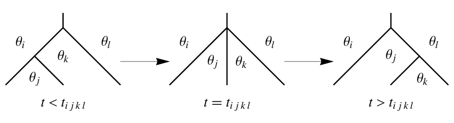
Figure 7: The evolution through a critical time $t_{ijkl}$ with visible critical point $P_{ijkl}$, where $p_{i}<p_{j}<p_{k}<p_{l}$. It amounts to a right-rotation (see e.g. [38]) applied to the first binary tree. This expresses a central feature of Tamari lattices, the rightward application of the associativity law mentioned in the introduction, in the language of binary trees (see also [23, 24, 26, 39, 32, 33]). It has to be considered as a local process, i.e. a binary tree displayed in this figure typically appears as a substructure of a bigger binary tree.

Proposition 3.4.

Let $p_{i}<p_{j}<p_{k}<p_{l}$. If $P_{ijkl}$ is visible at $t=t_{ijkl}$ and not a meeting point of more than four phases, then
(1) $P_{ijk}(t)$ and $P_{ikl}(t)$ are visible for $t<t_{ijkl}$,
(2) $P_{ijl}(t)$ and $P_{jkl}(t)$ are visible for $t>t_{ijkl}$.
Here $t$ is assumed to be close enough to $t_{ijkl}$ so that no other critical time with a visible critical point is in between.

Proof: For $t$ close enough to $t_{ijkl}$, a dominating phase in the vicinity of $P_{ijkl}$ can only be one of the four phases $\theta_{i},\theta_{j},\theta_{k},\theta_{l}$, as a consequence of the assumptions. As in the proof of Proposition 3.2, at $P_{ijl}(t)$ we have

$$\theta_{i}-\theta_{k}=(p_{k}-p_{i})(p_{k}-p_{j})(p_{l}-p_{k})(t-t_{ijkl})\,,$$

which is positive if $t>t_{ijkl}$. This excludes $\theta_{k}$ as a dominating phase. Since $\theta_{i}=\theta_{j}=\theta_{l}$ at $P_{ijl}(t)$, this critical point is visible. Clearly, $P_{ijl}(t)$ remains visible unless $t$ takes another critical value with a visible critical point. A similar argument applies to the other critical points. $\square$

Let us recall that, disregarding critical time values, any line soliton solution from the class defined in section 2 determines a time-ordered sequence of rooted binary trees (with the same number of leaves). Proposition 3.4 tells us that the rule according to which the transition from a binary tree to the next takes place is precisely the characteristic property of a Tamari lattice (see also Fig. 7). This leads to the following conclusion.

Theorem 3.5.

Each line soliton solution with $\tau$ of the form (2.1), $M>1$, and without coincidences of critical times defines a sequence of rooted binary trees which is a maximal chain in a Tamari lattice. $\square$

Up to $M=5$ we will show explicitly how every maximal chain in $\mathbb{T}_{M-1}$ is realized by line soliton solutions. Propositions 3.1, 3.2 and 3.4 have generalizations which are elaborated in Appendix Appendix A: Some general results and which will be important in the following. In particular, $x_{ij},y_{ijk},t_{ijkl}$ are special cases of (A.11).

Based on results of section 2 (in particular Propositions 2.2 and 2.3), a simple recipe to construct soliton binary trees can be formulated. A line soliton binary tree at a fixed time is indeed easily constructed from the sequence of ordered coordinates $y_{ijk}$ of the visible critical points $P_{ijk}$ via

$$x_{ik}\quad\stackrel{{\scriptstyle y_{ijk}}}{{\longrightarrow}}\quad(x_{ij},x_{jk})\,,$$ (3.3)

to be applied in the top to bottom direction (assuming $p_{i}<p_{j}<p_{k}$). Here we understand momentarily $x_{ij}$ to represent only the visible part of the line between (then dominating) phase regions $\theta_{i}$ and $\theta_{j}$. See Fig. 8 and also Appendix Appendix C: A symbolic representation of trees with levels, and a relation between permutohedra and Tamari lattices for further consequences.

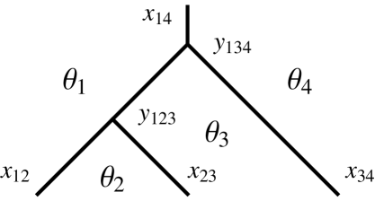
Figure 8: A binary tree constructed from the data $y_{134}>y_{123}$, starting with the root line $x_{14}$ and applying the branching rule (3.3) consecutively to the two nodes.

The transition to another binary tree at the critical time $t_{ijkl}$, i.e. the “rotation” shown in Fig. 7, can be expressed as

$$(y_{ikl},y_{ijk})\quad\stackrel{{\scriptstyle t_{ijkl}}}{{\longrightarrow}}\quad(y_{ijl},y_{jkl})\,,$$ (3.4)

assuming $p_{i}<p_{j}<p_{k}<p_{l}$. Here $(y_{ikl},y_{ijk})$ is a pair of neighbors in the decreasingly ordered sequence of critical $y$-values that determines a rooted binary tree associated with a line soliton solution at some event. In order to apply this map, it may be necessary to first apply a permutation (see Example 3.10 below and also Appendix Appendix C: A symbolic representation of trees with levels, and a relation between permutohedra and Tamari lattices). The initial rooted binary tree, corresponding to a line soliton solution at large negative values of $t$ (cf. Proposition 3.3), is determined by the sequence $(y_{1,M,M+1},y_{1,M-1,M},\ldots,y_{123})$. If we know the order of all critical times $t_{ijkl}$ that correspond to visible events, then (3.4) generates a description of the line soliton evolution as a chain of rooted binary trees.

Remark 3.6.

In section 2 we met a family of posets associated with simplexes, where the (directed) edges correspond to the critical values of $x$. There is a new family of posets where the nodes are given by the maximal chains in the corresponding poset of the first family. The (directed) edges are associated with the critical values of $y$, which are ordered increasingly from top to bottom along a chain. Now we note that the process determined by propositions 3.1, 3.2 and 3.4, hence (3.4), can be expressed as the graph in Fig. 9.

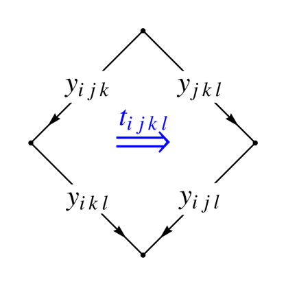
Figure 9: The process connected with the passage of $t$ through a visible critical value $t_{ijkl}$, where $p_{i}<p_{j}<p_{k}<p_{l}$. For $t<t_{ijkl}$ (left half of the figure), $y_{jkl}$ and $y_{ijl}$ are non-visible, whereas $y_{ijk}$ and $y_{ikl}$ are visible (at least if $t$ is greater than all other visible critical values that are smaller than $t_{ijkl}$). For $t>t_{ijkl}$ (right half of the figure), the latter pair becomes non-visible whereas $y_{jkl}$ and $y_{ijl}$ become visible (and remain visible at least until $t$ reaches the next critical value).

For $M=3$, Fig. 9 already displays the whole poset, which is thus a tetragon. The top node is given by the chain $x_{12}<x_{23}<x_{34}$, the left and right nodes by $x_{13}<x_{34}$ and $x_{12}<x_{24}$, respectively, and the bottom node by $x_{14}$. These data can be read off from the tetrahedron poset in Fig. 3. For $M=4$, we obtain the cube poset in Fig. 10. The top node is given by the longest maximal chain in the $M=4$ simplex poset of the first family, which is $x_{12}<x_{23}<x_{34}<x_{45}$. Using the rule expressed by the left graph of Fig. 3, the nodes in the next row are $x_{13}<x_{34}<x_{45}$, $x_{12}<x_{24}<x_{45}$ and $x_{12}<x_{23}<x_{35}$, respectively. In the next lower row we have $x_{14}<x_{45}$, $x_{13}<x_{35}$, and $x_{12}<x_{25}$. The bottom node is given by $x_{15}$. For $M>4$ we obtain a hypercube.

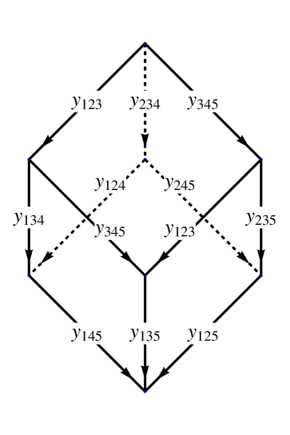
Figure 10: A poset with $M=4$. Five of its faces are associated with the critical values of $t$ according to the rule expressed in Fig. 9. The top face is an exception. It is associated with an additional kind of “critical value” of $t$, see Appendix Appendix B: A finer classification in terms of trees with levels.

For $t<\min\{t_{ijkl}\}$ we read off from the cube in Fig. 10 the chain $y_{123}<y_{134}<y_{145}$, which is the initial (rooted binary tree) configuration. If the first critical time is $t_{1234}$, then a transition to the tree determined by $y_{234}<y_{124}<y_{145}$ takes place, and for the further time development the only possibility is via the critical time $t_{1245}$ to $y_{234}<y_{245}<y_{125}$, and afterwards via $t_{2345}$ to $y_{345}<y_{235}<y_{125}$, which is the configuration for $t>\max\{t_{ijkl}\}$. If the first critical time is $t_{1345}$, then we have a transition to $y_{123}<y_{345}<y_{135}$. As a rooted binary tree, this is equivalent to the tree given by $y_{345}<y_{123}<y_{135}$, a transition encoded by the top face in Fig. 10. For the latter tree, the only possible further transition is via $t_{1235}$ to the unique final configuration for $t>\max\{t_{ijkl}\}$. All this results in the Tamari lattice $\mathbb{T}_{3}$ shown in Fig. 13 below. We will take a somewhat different route to it in order to be able to determine conditions under which the left or the right chain is realized, corresponding to which of the critical time values $t_{1234}$ and $t_{1345}$ is the smaller one.

3.2 The second step

To further classify the possible line soliton evolutions with $M>3$, we have to look at the cases where some of the critical times are equal. This corresponds to particular choices of the constants $c_{k}$. In order to analyze this, it turns out to be convenient to redefine the latter via

$$c_{k}\mapsto p_{k}^{4}\,t^{(4)}+c_{k}\qquad\quad k=1,\ldots,M+1\,,$$

with a new parameter $t^{(4)}$. If $t^{(4)}$ is identified with the next to $t$ evolution variable of the KP hierarchy, then the function $u$ (see section 2) also solves the second KP hierarchy equation. It should not be a big surprise that the hierarchy structure plays a simplifying role in the classification problem of line soliton solutions. Let us introduce the complete homogeneous symmetric polynomials

$$h_{m}(p_{i_{1}},\ldots,p_{i_{n}})=\sum_{\alpha_{1}+\cdots+\alpha_{n}=m}p_{i_{1}}^{\alpha_{1}}\,p_{i_{2}}^{\alpha_{2}}\cdots\,p_{i_{n}}^{\alpha_{n}}\,,$$

where $\alpha_{k}\in\mathbb{N}\cup\{0\}$. Then we have (see also (A.11))

$$x_{ij}(y,t,t^{(4)}) = -h_{1}(p_{i},p_{j})\,y-h_{2}(p_{i},p_{j})\,t-h_{3}(p_{i},p_{j})\,t^{(4)}-c_{ij}\,,$$

$$x_{ijk}(t,t^{(4)}) = x_{ij}(y_{ijk}(t,t^{(4)}),t,t^{(4)})\,,$$

$$y_{ijk}(t,t^{(4)}) = -h_{1}(p_{i},p_{j},p_{k})\,t-h_{2}(p_{i},p_{j},p_{k})\,t^{(4)}-c_{ijk}\,,$$

$$t_{ijkl}(t^{(4)}) = -h_{1}(p_{i},p_{j},p_{k},p_{l})\,t^{(4)}-c_{ijkl}\,,$$

with $c_{ij},c_{ijk}$ and $c_{ijkl}$ given in terms of $c_{i}$ by the previous formulae. We note that now a critical point $P_{ijk}$ depends on $t$ and $t^{(4)}$, hence it forms a surface in $\mathbb{R}^{4}$. The critical point $P_{ijkl}$ depends on $t^{(4)}$, hence it forms a line in $\mathbb{R}^{4}$, which is the intersection of the surfaces corresponding to $P_{ijk},P_{ikl},P_{ijl},P_{jkl}$.

We find (see also Proposition A.3)

$$t_{ijkl}(t^{(4)})-t_{ijkm}(t^{(4)})=(p_{m}-p_{l})(t^{(4)}-t^{(4)}_{ijklm})\qquad\mbox{with}\quad t^{(4)}_{ijklm}=-c_{ijklm}\,,$$ (3.5)

where

$$c_{ijklm}=\frac{c_{ijkl}-c_{ijkm}}{p_{l}-p_{m}}=\frac{c_{i}}{(p_{i}-p_{j})(p_{i}-p_{k})(p_{i}-p_{l})(p_{i}-p_{m})}+\mbox{cyclic permutations}\;.$$

If two critical times sharing three indices are equal, i.e. $t_{ijkl}=t_{ijkm}$, then it follows that (at least) five critical times are equal: $t_{ijkl}=t_{ijkm}=t_{ijlm}=t_{iklm}=t_{jklm}$. This happens when $t^{(4)}=t^{(4)}_{ijklm}$. At the critical event

$$(P_{ijklm},t_{ijkl}(t^{(4)}_{ijklm}),t^{(4)}_{ijklm})\in\mathbb{R}^{4}\,,$$

with projection point

$$P_{ijklm}:=P_{ijkl}(t^{(4)}_{ijklm})$$

in the $xy$-plane, we thus have $\theta_{i}=\theta_{j}=\theta_{k}=\theta_{l}=\theta_{m}$. The following is a direct consequence of (3.5) (see also Proposition A.4).

Proposition 3.7.

If $p_{i}<p_{j}<p_{k}<p_{l}<p_{m}$ we have

$$\begin{array}[]{l}t_{ijkl}(t^{(4)})<t_{ijkm}(t^{(4)})<t_{ijlm}(t^{(4)})<t_{iklm}(t^{(4)})<t_{jklm}(t^{(4)})\\ t_{ijkl}(t^{(4)})>t_{ijkm}(t^{(4)})>t_{ijlm}(t^{(4)})>t_{iklm}(t^{(4)})>t_{jklm}(t^{(4)})\end{array}\quad\mbox{for}\quad\begin{array}[]{l}t^{(4)}<t^{(4)}_{ijklm}\\ t^{(4)}>t^{(4)}_{ijklm}\end{array}\;.$$

$\square$

The next results are special cases of Propositions A.7 and A.8 in Appendix Appendix A: Some general results.

Proposition 3.8.

Let $p_{i}<p_{j}<p_{k}<p_{l}<p_{m}$. Then
(1) $P_{iklm}(t^{(4)})$ and $P_{ijkm}(t^{(4)})$ are non-visible for $t^{(4)}<t^{(4)}_{ijklm}$.
(2) $P_{ijkl}(t^{(4)}),P_{ijlm}(t^{(4)})$ and $P_{jklm}(t^{(4)})$ are non-visible for $t^{(4)}>t^{(4)}_{ijklm}$. $\square$

Proposition 3.9.

Let $p_{i}<p_{j}<p_{k}<p_{l}<p_{m}$ and suppose $P_{ijklm}$ is visible at $t=t_{ijkl}$, $t^{(4)}=t^{(4)}_{ijklm}$, and not a meeting point of more than five phases. The following holds for values of $t^{(4)}$ that are close enough to $t^{(4)}_{ijklm}$, so that no other critical value of $t^{(4)}$ with visible projection point is in between.
(1) $P_{ijkl}(t^{(4)}),P_{ijlm}(t^{(4)})$ and $P_{jklm}(t^{(4)})$ are visible, at the respective critical time, if $t^{(4)}<t^{(4)}_{ijklm}$.
(2) $P_{iklm}(t^{(4)})$ and $P_{ijkm}(t^{(4)})$ are visible, at the respective critical time, if $t^{(4)}>t^{(4)}_{ijklm}$. $\square$

Fig. 11 expresses the subgraph structure determined by Propositions 3.7, 3.8 and 3.9 as a process.

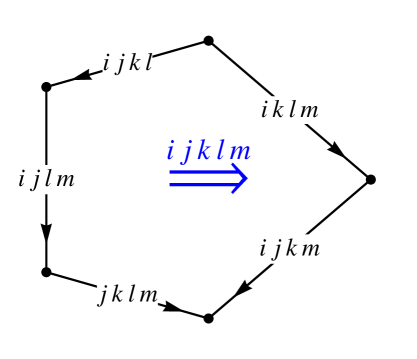
Figure 11: The process connected with the passage of $t^{(4)}$ through a critical value $t^{(4)}_{ijklm}$ with visible critical point $P_{ijklm}$, where $p_{i}<p_{j}<p_{k}<p_{l}<p_{m}$. Here $ijkl$ stands for $t_{ijkl}$ and $ijklm$ for $t^{(4)}_{ijklm}$. The left chain corresponds to $t^{(4)}<t^{(4)}_{ijklm}$, the right to $t^{(4)}>t^{(4)}_{ijklm}$. See also Fig. 13 for a special case.

Example 3.10.

Let $M=4$. For any fixed $t^{(4)}$, we have five critical times $t_{1234}(t^{(4)})$, $t_{1235}(t^{(4)})$, $t_{1245}(t^{(4)})$, $t_{1345}(t^{(4)})$, $t_{2345}(t^{(4)})$. The corresponding critical events have projection points $P_{1234}(t^{(4)})$, $P_{1235}(t^{(4)})$, $P_{1245}(t^{(4)})$, $P_{1345}(t^{(4)})$, $P_{2345}(t^{(4)})$, at which four phases meet. All these critical events coincide for $t^{(4)}=t^{(4)}_{12345}$. At the associated projection point $P_{12345}$ all the five phases meet, and it is therefore visible at $t=t_{1234}$ and $t^{(4)}=t^{(4)}_{12345}$. A description of the evolution of the line soliton pattern thus has to distinguish the cases $t^{(4)}<t^{(4)}_{12345}$ and $t^{(4)}>t^{(4)}_{12345}$.
(1) $t^{(4)}<t^{(4)}_{12345}$. From Propositions 3.7, 3.8 and 3.9, we obtain all “visible” critical times and they satisfy $t_{1234}<t_{1245}<t_{2345}$. Via (3.4) this yields

$$(y_{145},y_{134},y_{123})\stackrel{{\scriptstyle t_{1234}}}{{\longrightarrow}}(y_{145},y_{124},y_{234})\stackrel{{\scriptstyle t_{1245}}}{{\longrightarrow}}(y_{125},y_{245},y_{234})\stackrel{{\scriptstyle t_{2345}}}{{\longrightarrow}}(y_{125},y_{235},y_{345})\,,$$

which translates into the first sequence of rooted binary trees in Fig. 12.

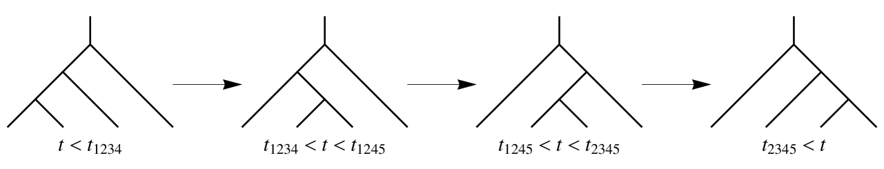
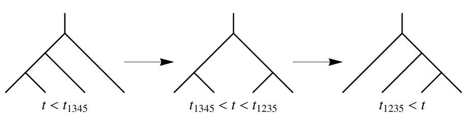
Figure 12: Evolution of line soliton patterns with $M=4$ and $t^{(4)}<t^{(4)}_{12345}$ (first chain), respectively $t^{(4)}>t^{(4)}_{12345}$ (second chain). These are the two maximal chains in the Tamari lattice $\mathbb{T}_{3}$, which forms a pentagon (see Fig. 13). Instead of assigning $t$-intervals to the trees, it is convenient to assign the corresponding critical values $t_{ijkl}$ to the arrows, i.e. the edges of the Tamari lattice (as in Figs. 11 and 13).

(2) $t^{(4)}>t^{(4)}_{12345}$. Then the “visible” critical times satisfy $t_{1345}<t_{1235}$. This leads to

$$(y_{145},y_{134},y_{123})\stackrel{{\scriptstyle t_{1345}}}{{\longrightarrow}}(y_{135},y_{345},y_{123})\stackrel{{\scriptstyle\mathrm{permutation}}}{{\longrightarrow}}(y_{135},y_{123},y_{345})\stackrel{{\scriptstyle t_{1235}}}{{\longrightarrow}}(y_{125},y_{235},y_{345})\,,$$

which translates into the second chain in Fig. 12. The tree in the middle allows the two possibilities $y_{123}<y_{345}$ and $y_{345}<y_{123}$ (in accordance with Proposition 3.1). A permutation is necessary in order to be able to apply (3.4) with the second critical time to the respective pair of neighbors. This makes sense if we regard the two possibilities as equivalent (and this has been done in Fig. 12). Resolving the “fine structure”, by determining the event where $y_{123}=y_{345}$, they can be distinguished in a setting of trees with levels [30], see Appendix Appendix B: A finer classification in terms of trees with levels.
The two sequences of rooted binary trees obtained for $t^{(4)}<t^{(4)}_{12345}$, respectively $t^{(4)}>t^{(4)}_{12345}$, are the two maximal chains in the Tamari lattice $\mathbb{T}_{3}$ (see Fig. 13).

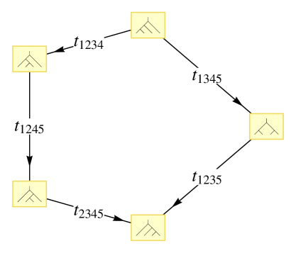
Figure 13: Representation of the Tamari lattice $\mathbb{T}_{3}$ by line soliton graphs (which is a special case of Fig. 11, see also Remark 3.6). The left chain is realized if $t^{(4)}<t^{(4)}_{12345}$, the right chain if $t^{(4)}>t^{(4)}_{12345}$ (see also Fig. 12). At $t=t_{1234}(t^{(4)}_{12345})$ and $t^{(4)}=t^{(4)}_{12345}$, a direct transition takes place from the uppermost to the lowermost tree.

3.3 The third step

For $M>4$ we redefine the constants $c_{k}$ once more,

$$c_{k}\mapsto p_{k}^{5}\,t^{(5)}+c_{k}\qquad\quad k=1,\ldots,M+1\,,$$

with a new parameter $t^{(5)}$. Then we have

$$x_{ij}(y,t,t^{(4)},t^{(5)}) = -h_{1}(p_{i},p_{j})\,y-h_{2}(p_{i},p_{j})\,t-h_{3}(p_{i},p_{j})\,t^{(4)}-h_{4}(p_{i},p_{j})\,t^{(5)}-c_{ij}\,,$$

$$x_{ijk}(t,t^{(4)},t^{(5)}) = x_{ij}(y_{ijk}(t,t^{(4)},t^{(5)}),t,t^{(4)},t^{(5)})\,,$$

$$y_{ijk}(t,t^{(4)},t^{(5)}) = -h_{1}(p_{i},p_{j},p_{k})\,t-h_{2}(p_{i},p_{j},p_{k})\,t^{(4)}-h_{3}(p_{i},p_{j},p_{k})\,t^{(5)}-c_{ijk}\,,$$

$$t_{ijkl}(t^{(4)},t^{(5)}) = h_{1}(p_{i},p_{j},p_{k},p_{l})\,t^{(4)}-h_{2}(p_{i},p_{j},p_{k},p_{l})\,t^{(5)}-c_{ijkl}\,,$$

$$t^{(4)}_{ijklm}(t^{(5)}) = -h_{1}(p_{i},p_{j},p_{k},p_{l},p_{m})\,t^{(5)}-c_{ijklm}\,,$$

with $c_{ij}$, $c_{ijk}$, $c_{ijkl}$ and $c_{ijklm}$ as defined previously (see also (A.9)). Coincidences of critical values of $t^{(4)}$ can only occur at the following critical values of $t^{(5)}$,

$$t^{(5)}_{ijklmn}=-c_{ijklmn}\,,$$

where

$$c_{ijklmn}=\frac{c_{ijklm}-c_{ijkln}}{p_{m}-p_{n}}=\frac{c_{i}}{(p_{i}-p_{j})(p_{i}-p_{k})(p_{i}-p_{l})(p_{i}-p_{m})(p_{i}-p_{n})}+\mbox{cyclic permutations}\;.$$

This follows from the identity (see also Proposition A.3)

$$t^{(4)}_{ijklm}-t^{(4)}_{ijkln}=(p_{n}-p_{m})(t^{(5)}-t^{(5)}_{ijklmn})\;.$$ (3.7)

Furthermore, at $t^{(5)}=t^{(5)}_{ijklmn}$ we have $t^{(4)}_{ijklm}=t^{(4)}_{ijkln}=t^{(4)}_{ijkmn}=t^{(4)}_{ijlmn}=t^{(4)}_{iklmn}=t^{(4)}_{jklmn}$. At this critical event (now a point in $\mathbb{R}^{5}$ with coordinates $x,y,t,t^{(4)},t^{(5)}$) having the projection

$$P_{ijklmn}:=P_{ijklm}(t^{(5)}_{ijklmn})$$

in the $xy$-plane, we have $\theta_{i}=\theta_{j}=\theta_{k}=\theta_{l}=\theta_{m}=\theta_{n}$. The following is a consequence of (3.7) (see also Proposition A.4).

Proposition 3.11.

If $p_{i}<p_{j}<p_{k}<p_{l}<p_{m}<p_{n}$, then

$$\begin{array}[]{l}t^{(4)}_{ijklm}<t^{(4)}_{ijkln}<t^{(4)}_{ijkmn}<t^{(4)}_{ijlmn}<t^{(4)}_{iklmn}<t^{(4)}_{jklmn}\\ t^{(4)}_{ijklm}>t^{(4)}_{ijkln}>t^{(4)}_{ijkmn}>t^{(4)}_{ijlmn}>t^{(4)}_{iklmn}>t^{(4)}_{jklmn}\end{array}\quad\mbox{for}\quad\begin{array}[]{l}t^{(5)}<t^{(5)}_{ijklmn}\\ t^{(5)}>t^{(5)}_{ijklmn}\end{array}\;.$$

$\square$

The next two propositions are special cases of Proposition A.7 and A.8, respectively.

Proposition 3.12.

Let $p_{i}<p_{j}<p_{k}<p_{l}<p_{m}<p_{n}$. Then
(1) $P_{ijkln}(t^{(5)}),P_{ijlmn}(t^{(5)})$ and $P_{jklmn}(t^{(5)})$ are non-visible for $t^{(5)}<t^{(5)}_{ijklmn}$.
(2) $P_{ijklm}(t^{(5)}),P_{ijkmn}(t^{(5)})$ and $P_{iklmn}(t^{(5)})$ are non-visible for $t^{(5)}>t^{(5)}_{ijklmn}$. $\square$

Proposition 3.13.

Let $p_{i}<p_{j}<p_{k}<p_{l}<p_{m}<p_{n}$ and suppose that $P_{ijklmn}$ is visible at $t=t_{ijkl}$, $t^{(4)}=t^{(4)}_{ijklm}$, $t^{(5)}=t^{(5)}_{ijklmn}$, and not a meeting point of more than six phases. The following holds for values of $t^{(5)}$ that are close enough to $t^{(5)}_{ijklmn}$, so that no other critical value of $t^{(5)}$ with visible projection point is in between.
(1) $P_{ijklm}(t^{(5)})$, $P_{ijkmn}(t^{(5)})$ and $P_{iklmn}(t^{(5)})$ are visible, at the respective critical values of $t$ and $t^{(4)}$, if $t^{(5)}<t^{(5)}_{ijklmn}$.
(2) $P_{jklmn}(t^{(5)}),P_{ijlmn}(t^{(5)})$ and $P_{ijkln}(t^{(5)})$ are visible, at the respective critical values of $t$ and $t^{(4)}$, if $t^{(5)}>t^{(5)}_{ijklmn}$. $\square$

Fig. 14 expresses a consequence of Propositions 3.11, 3.12 and 3.13 as a process.

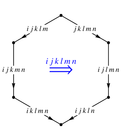
Figure 14: The process connected with the passage of $t^{(5)}$ through a critical value $t^{(5)}_{ijklmn}$ with a visible critical event, where $p_{i}<p_{j}<p_{k}<p_{l}<p_{m}<p_{n}$. Here $ijklm$ stands for $t^{(4)}_{ijklm}$ and $ijklmn$ for $t^{(5)}_{ijklmn}$. The left chain corresponds to $t^{(5)}<t^{(5)}_{ijklmn}$, the right to $t^{(5)}>t^{(5)}_{ijklmn}$. The nodes are classes of chains in a Tamari lattice, see Example 3.14.

Example 3.14.

For $M=5$ there is only a single critical value of $t^{(5)}$, namely $t^{(5)}_{123456}$, and $P_{123456}$ is visible at $t=t_{1234}$, $t^{(4)}=t^{(4)}_{12345}$ and $t^{(5)}=t^{(5)}_{123456}$, as a meeting point of all six phases. There are six critical values of $t^{(4)}$, namely $t^{(4)}_{12345},t^{(4)}_{12346},t^{(4)}_{12356},t^{(4)}_{12456},t^{(4)}_{13456},t^{(4)}_{23456}$. For $t^{(5)}<t^{(5)}_{123456}$, according to Proposition 3.11 we have to distinguish the cases where (1) $t^{(4)}<t^{(4)}_{12345}$, (2) $t^{(4)}_{12345}<t^{(4)}<t^{(4)}_{12356}$, (3) $t^{(4)}_{12356}<t^{(4)}<t^{(4)}_{13456}$, and (4) $t^{(4)}_{13456}<t^{(4)}$.
In case (1) we obtain from Proposition 3.7 the inequalities (a) $t_{1234}<t_{1235}<t_{1245}<t_{1345}<t_{2345}$, (b) $t_{1234}<t_{1236}<t_{1246}<t_{1346}<t_{2346}$, (c) $t_{1235}<t_{1236}<t_{1256}<t_{1356}<t_{2356}$, (d) $t_{1245}<t_{1246}<t_{1256}<t_{1456}<t_{2456}$, (e) $t_{1345}<t_{1346}<t_{1356}<t_{1456}<t_{3456}$, (f) $t_{2345}<t_{2346}<t_{2356}<t_{2456}<t_{3456}$. According to Proposition 3.8, the critical points appearing at the times $t_{1235}$, $t_{1236}$, $t_{1246}$, $t_{1345}$, $t_{1346}$, $t_{1356}$, $t_{1456}$, $t_{2346}$, $t_{2456}$ are non-visible. Their elimination leads to (a) $t_{1234}<t_{1245}<t_{2345}$, (b) $t_{1234}$, (c) $t_{1256}<t_{2356}$, (d) $t_{1245}<t_{1256}$, (e) $t_{3456}$, (f) $t_{2345}<t_{2356}<t_{3456}$, and the union determines the second poset in Fig. 15. Since Proposition A.9 does not identify any of the remaining critical times as “non-visible” (note that $t^{(4)}_{12345}$, $t^{(4)}_{12356}$ and $t^{(4)}_{13456}$ correspond to visible events according to Proposition 3.13), we can refer to Proposition A.10 in order to conclude that they all correspond to visible events only.

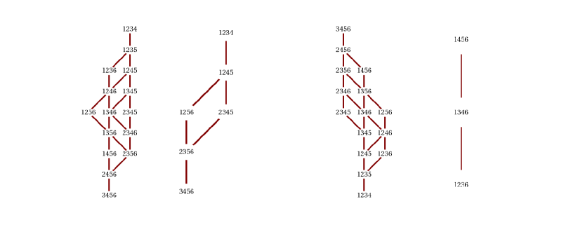
Figure 15: Intermediate step in the derivation of the possible line soliton evolutions for $M=5$ and $t^{(4)}<\min\{t^{(4)}_{ijklm}\}$ (pair of posets on the left), respectively $t^{(4)}>\max\{t^{(4)}_{ijklm}\}$ (pair of posets on the right). In both cases the first diagram is obtained as the union of all sequences of ordered critical times. The second diagram then results by dropping those critical times for which the critical event (or rather its projection in the $xy$-plane) is non-visible (and removing redundant edges). A four-digit number stands for the corresponding critical time.

Depending on the order of the critical time values $t_{1256}$ and $t_{2345}$, the evolution follows one of the two sequences of rooted binary trees in Fig. 16, easily elaborated with the help of (3.4).

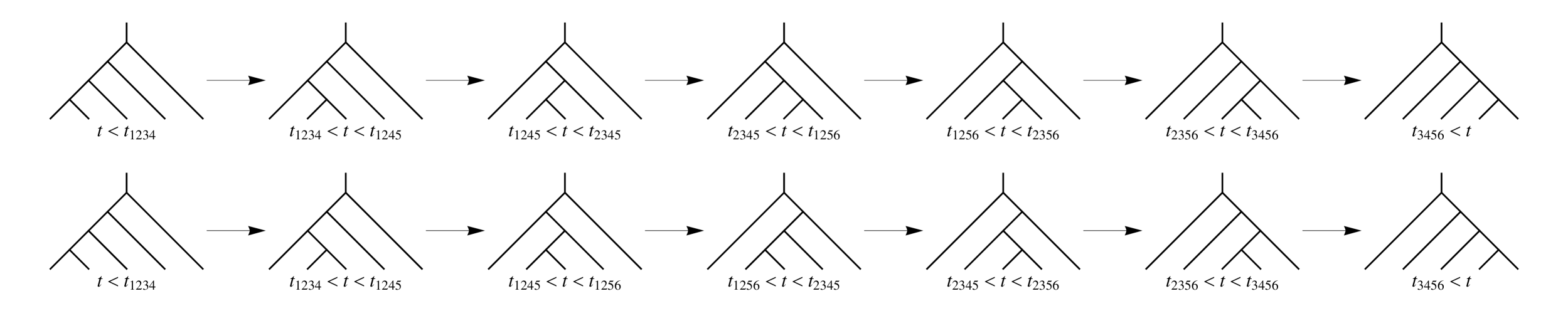
Figure 16: The two possible evolutions for $M=5$ and $t^{(4)}<\min\{t^{(4)}_{ijklm}\}$. They correspond to chains in the Tamari lattice $\mathbb{T}_{4}$.

In case (4) we have the inequalities (a’) $t_{1234}>t_{1235}>t_{1245}>t_{1345}>t_{2345}$, (b’) $t_{1234}>t_{1236}>t_{1246}>t_{1346}>t_{2346}$, (c’) $t_{1235}>t_{1236}>t_{1256}>t_{1356}>t_{2356}$, (d’) $t_{1245}>t_{1246}>t_{1256}>t_{1456}>t_{2456}$, (e’) $t_{1345}>t_{1346}>t_{1356}>t_{1456}>t_{3456}$, (f’) $t_{2345}>t_{2346}>t_{2356}>t_{2456}>t_{3456}$. Now we have to eliminate $t_{1234}$, $t_{1235}$, $t_{1245}$, $t_{1246}$, $t_{1256}$, $t_{1345}$, $t_{1356}$, $t_{2345}$, $t_{2346}$, $t_{2356}$, $t_{2456}$, $t_{3456}$ (see Fig. 15). The resulting sequence of rooted binary trees is shown in Fig. 17.

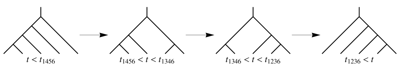
Figure 17: The evolution for $M=5$ and $t^{(4)}>\max\{t^{(4)}_{ijklm}\}$, another chain in the Tamari lattice $\mathbb{T}_{4}$.

Fig. 18 shows the resulting classes of chains in the cases (1)-(4).

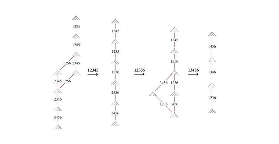
Figure 18: Classes of possible evolutions for $M=5$ and $t^{(5)}<t^{(5)}_{123456}$, corresponding to intervals of $t^{(4)}$ and transitions at critical values of $t^{(4)}$. This corresponds to the left chain in Fig. 14.

For $t^{(5)}>t^{(5)}_{123456}$, the corresponding (classes of) chains are displayed in Fig. 19. Collecting all different chains, we obtain the representation of the Tamari lattice $\mathbb{T}_{4}$ in Fig. 20.

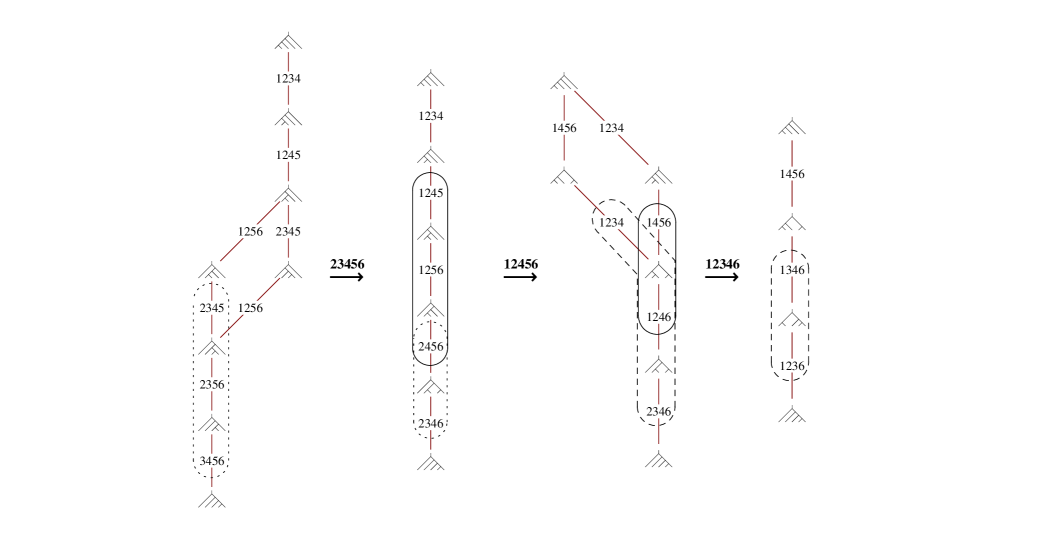
Figure 19: Classes of possible evolutions for $M=5$ and $t^{(5)}>t^{(5)}_{123456}$. This corresponds to the right chain in Fig. 14. As indicated by equally encircled parts, the deformation of a class into the next, as $t^{(4)}$ passes through a critical value, proceeds according to the left to right half pentagon structure of $\mathbb{T}_{3}$.

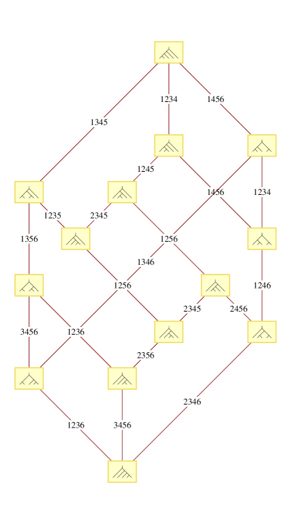
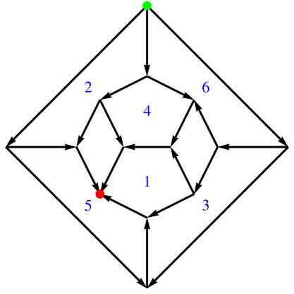
Figure 20: The left graph shows the representation of the Tamari lattice $\mathbb{T}_{4}$ in terms of rooted binary trees which represent line soliton patterns. The digraph on the right describes $\mathbb{T}_{4}$ without overlapping edges and makes evident that it consists of six pentagons and three tetragons. (The 2-faces of Tamari lattices are pentagons or tetragons, see e.g. [40].) Here the numbers assigned to the pentagons encode the critical times associated with the edges. For an edge between pentagon $i$ and pentagon $j$ we form the complement of $ij$ in $123456$, which then determines the associated critical time. Opposite edges of a tetragon have to be identified for this counting, so that e.g. $t_{1456}$ is assigned to the left uppermost arrow. Another familiar representation is as a poset structure on the associahedron [41, 42, 43] in three dimensions.

In order to realize a certain chain in $\mathbb{T}_{4}$, the critical times appearing along it all have to be smaller than the critical times of neighboring branches. Solving the inequalities arising in this way, one obtains the conditions in Table 1 (see also Tables 2 and 3 in Appendix Appendix B: A finer classification in terms of trees with levels). An example of a line soliton solution of type 1 in the table is displayed in Fig. 21.

1	$t_{1234},t_{1245},t_{2345},t_{1256},t_{2356},t_{3456}$	$\mu<0$	$\frac{p_{3}+p_{4}-p_{1}-p_{6}}{(p_{3}-p_{6})(p_{4}-p_{6})}<\lambda/\mu$
2	$t_{1234},t_{1245},t_{1256},t_{2345},t_{2356},t_{3456}$		$\frac{1}{p_{1}-p_{6}}<\lambda/\mu<\frac{p_{3}+p_{4}-p_{1}-p_{6}}{(p_{3}-p_{6})(p_{4}-p_{6})}$
3	$t_{1234},t_{1245},t_{1256},t_{2456},t_{2346}$		$\frac{1}{p_{3}-p_{6}}<\lambda/\mu<\frac{1}{p_{1}-p_{6}}$
4	$t_{1234},t_{1456},t_{1246},t_{2346}$		$\frac{p_{2}+p_{3}-p_{5}-p_{6}}{(p_{2}-p_{6})(p_{3}-p_{6})}<\lambda/\mu<\frac{1}{p_{3}-p_{6}}$
5	$t_{1456},t_{1234},t_{1246},t_{2346}$		$\frac{1}{p_{5}-p_{6}}<\lambda/\mu<\frac{p_{2}+p_{3}-p_{5}-p_{6}}{(p_{2}-p_{6})(p_{3}-p_{6})}$
6	$t_{1456},t_{1346},t_{1236}$	$\mu\leq 0$	$\frac{1}{p_{5}-p_{6}}\mu<\lambda$
		$\mu>0$	$\frac{1}{p_{2}-p_{6}}<\lambda/\mu$
7	$t_{1345},t_{1356},t_{3456},t_{1236}$		$\frac{p_{1}+p_{2}-p_{4}-p_{5}}{p_{1}p_{2}-p_{4}p_{5}+(p_{4}+p_{5}-p_{1}-p_{2})\,p_{6}}<\lambda/\mu<\frac{1}{p_{2}-p_{6}}$
8	$t_{1345},t_{1356},t_{1236},t_{3456}$		$\frac{1}{p_{4}-p_{6}}<\lambda/\mu<\frac{p_{1}+p_{2}-p_{4}-p_{5}}{p_{1}p_{2}-p_{4}p_{5}+(p_{4}+p_{5}-p_{1}-p_{2})\,p_{6}}$
9	$t_{1345},t_{1235},t_{1256},t_{2356},t_{3456}$		$\lambda/\mu<\frac{1}{p_{4}-p_{6}}$

Table 1: The nine maximal chains in the Tamari lattice $\mathbb{T}_{4}$, here described by the corresponding sequences of critical times $t_{ijkl}$, and the parameter conditions under which they occur. We set $\mu=t^{(4)}-t^{(4)}_{12345}$ and $\lambda=t^{(5)}-t^{(5)}_{123456}$. Recall that $p_{1}<p_{2}<p_{3}<p_{4}<p_{5}<p_{6}$.

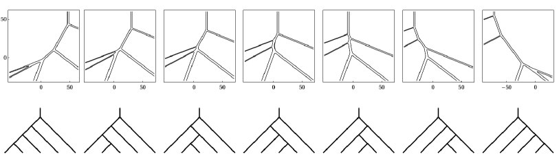
Figure 21: The evolution of a line soliton pattern of type 1 in Table 1. Here we have $\theta_{i}=p_{i}x+p_{i}^{2}y+p_{i}^{3}t+p_{i}^{4}t^{(4)}+p_{i}^{5}t^{(5)}+c_{i}$ with the choice $p_{1}=-2,p_{2}=-3/2,p_{3}=-1,p_{4}=1/2,p_{5}=5/4,p_{6}=2$ and $c_{1}=10,c_{2}=c_{3}=c_{4}=c_{5}=0,c_{6}=-10$. Furthermore, we set $\mu=-2$ and $\lambda=-1$. The line soliton plots are taken at $t=-10,-5.7,-3.6,0,4,10,20$.

The further steps needed to treat the cases $M>5$ should now be obvious and we refer to Appendix Appendix A: Some general results for corresponding general results.

4 On the general class of KP line soliton solutions

In the preceding sections (and Appendix Appendix A: Some general results) we restricted our considerations to a special class of line soliton solutions and achieved a complete description (in the tropical approximation) of their evolution. In this section we argue that more general solutions can actually be understood fairly well as superimpositions of solutions from the special class, with rather simple modifications. The somewhat qualitative picture layed out in this section still has to be elaborated in more detail, however.

The general class of line soliton solutions of the KP-II equation (and more generally its hierarchy) in Hirota form is well-known to be given by

$$\tau=f_{1}\wedge f_{2}\wedge\cdots\wedge f_{n}\,,$$

where

$$f_{i}=\sum_{j=1}^{M+1}\epsilon_{ij}\,e_{j}\,,\qquad e_{j}=e^{\theta_{j}}\,,\qquad\theta_{j}=\sum_{r=1}^{M}p_{j}^{r}\,t^{(r)}+c_{j}\,,$$

and the exterior product on the space of functions generated by the exponential functions $e_{j}$, $j=1,\ldots,M+1$, is defined by

$$e_{i_{1}}\wedge\cdots\wedge e_{i_{m}}=\Delta(p_{i_{1}},\ldots,p_{i_{m}})\,e_{i_{1}}\cdots e_{i_{m}}\,,$$

with the Vandermonde determinant (A.7). Hence

$$\tau=\sum_{1\leq i_{1}<\cdots<i_{n}\leq M+1}A_{i_{1}\ldots i_{n}}\,e_{i_{1}}\cdots e_{i_{n}}\quad\mbox{where}\quad A_{i_{1}\ldots i_{n}}=\epsilon_{1i_{1}}\cdots\epsilon_{ni_{n}}\,\Delta(p_{i_{1}},\ldots,p_{i_{n}})\;.$$

Example 4.1.

A subclass of the above class of solutions is given by

$$\tau = (e_{1}+e_{2})\wedge(e_{2}+e_{3})\wedge\cdots\wedge(e_{M}+e_{M+1})$$

$$= \sum_{i=1}^{M+1}e_{1}\wedge\cdots\wedge\widehat{e_{i}}\wedge e_{i+1}\wedge\cdots\wedge e_{M+1}$$

$$= \Delta(p_{1},\ldots,p_{M+1})\,e^{\theta_{1}+\cdots+\theta_{M+1}}\,\sum_{i=1}^{M+1}a_{i}\,e^{-\theta_{i}}\,,$$

where a hat indicates an omission, and $a_{i}=1/[(p_{i}-p_{1})\cdots(p_{i}-p_{i-1})(p_{i+1}-p_{i})\cdots(p_{M+1}-p_{i})]$. Assuming $p_{1}<p_{2}<\cdots<p_{M+1}$, $a_{i}$ is positive, hence it can be absorbed into the constant $c_{i}$. Moreover, the factor in front of the sum drops out in the expression $u=2\log(\tau)_{xx}$ for the KP soliton solution, so that an equivalent $\tau$-function is given by

$$\tilde{\tau}=\sum_{i=1}^{M+1}e^{-\theta_{i}}\;.$$

Via $p_{i}\mapsto-p_{i}$ and $c_{i}\mapsto-c_{i}$ (and with a renumbering of the $p$’s), this is the class of solutions treated in the main part of this work, up to the reflection $t^{(2r)}\mapsto-t^{(2r)}$, $r=1,2,\ldots$, which includes $y\mapsto-y$. The corresponding rooted binary trees are hence given by those of our simple class, but drawn upside down.

Remark 4.2.

Since the above expression for $\tau$ determines a KP solution, this also holds for

$$\tau^{\prime}=e^{-\theta_{1}-\cdots-\theta_{M+1}}\,\tau=\sum_{1\leq i_{1}<\cdots<i_{n}\leq M+1}A_{i_{1}\ldots i_{n}}\,e^{-\theta_{k_{1}}-\cdots-\theta_{k_{n^{\prime}}}}\,,$$

where $\{k_{1},\ldots,k_{n^{\prime}}\}=\{1,\ldots,M+1\}\setminus\{i_{1},\ldots,i_{n}\}$. Since the reflection $t^{(r)}\mapsto-t^{(r)}$, $r=1,2,\ldots$, is a symmetry of the KP equation, and since $c_{i}\mapsto-c_{i}$ preserves the above class of solutions, we conclude that also

$$\tau_{\star}=\sum_{1\leq i_{1}<\cdots<i_{n}\leq M+1}A_{i_{1}\ldots i_{n}}\,e^{\theta_{k_{1}}+\cdots+\theta_{k_{n^{\prime}}}}=\sum_{1\leq i_{1}<\cdots<i_{n}\leq M+1}A_{i_{1}\ldots i_{n}}\,e_{k_{1}}\cdots e_{k_{n^{\prime}}}$$

is a solution, which we call the dual of $\tau$.

Let us order the constants $p_{i}$ such that $p_{1}<\cdots<p_{M+1}$ and let us assume that no pair of the functions $f_{i}$, $i=1,\ldots,n$, has an $e_{j}$ in common. The cases excluded by this assumption can be recovered by taking a limit where pairs of neighboring $p$’s coincide. By absorbing the modulus of a nonvanishing constant $\epsilon_{ij}$ via a redefinition of the constant $c_{j}$, without restriction of generality we can assume that

$$\epsilon_{ij}\in\{0,\pm 1\}\;.$$

By demanding that the coefficients $A_{i_{1}\ldots i_{n}}$ are all non-negative, and at least one of them different from zero, we ensure that $\tau$ is positive and the KP solution is then regular. Then we obtain

$$\tau=\sum_{1\leq i_{1}<\cdots<i_{n}\leq M+1}|\epsilon_{1i_{1}}\cdots\epsilon_{ni_{n}}|\;e^{\theta_{i_{1}\ldots i_{n}}}\,,$$

where

$$\theta_{i_{1}\ldots i_{n}}=\theta_{i_{1}}+\cdots+\theta_{i_{n}}+\log\Delta(p_{i_{1}},\ldots,p_{i_{n}})\;.$$

In particular,

$$\theta_{ij}=\theta_{i}+\theta_{j}+\log(p_{j}-p_{i})\;.$$

For fixed values of the parameters $t^{(3)}=t,t^{(4)},\ldots$, the $xy$-plane is divided into regions where one of the phases $\theta_{i_{1}\ldots i_{n}}$ dominates all others. The line soliton segments are given by the visible boundaries of these regions. The tropical approximation now reads

$$\log(\tau)\simeq\max\{\theta_{i_{1}\ldots i_{n}}\,|\,1\leq i_{1}<\cdots<i_{n}\leq M+1,\,\epsilon_{1i_{1}}\cdots\epsilon_{ni_{n}}\neq 0\}\;.$$

In principle one can approach a classification of solutions in a similar way as done for the special class in the main part of this work. In the following we set $t^{(n)}=0$ for $n>3$ (more precisely, we absorb these variables into the constants $c_{i}$). Assuming $p_{i}<p_{j}$, $p_{k}<p_{l}$ and $p_{i}+p_{j}\neq p_{k}+p_{l}$, we have

$$\theta_{ij}-\theta_{kl}=(p_{i}+p_{j}-p_{k}-p_{l})(x-x_{ij,kl}(y,t))\,,$$ (4.1)

where

$$x_{ij,kl}(y,t) = \frac{1}{p_{i}+p_{j}-p_{k}-p_{l}}\Big{(}-(p_{i}^{2}+p_{j}^{2}-p_{k}^{2}-p_{l}^{2})\,y-(p_{i}^{3}+p_{j}^{3}-p_{k}^{3}-p_{l}^{3})\,t$$ (4.2)

$$-c_{i}-c_{j}+c_{k}+c_{l}+\log\Big{(}\frac{p_{l}-p_{k}}{p_{j}-p_{i}}\Big{)}\Big{)}\;.$$

The boundary between the regions associated with the two phases $\theta_{ij}$ and $\theta_{kl}$ is therefore given by $x=x_{ij,kl}(y,t)$. In particular, we find that

$$x_{ik,jk}=x_{ij}+\frac{1}{p_{j}-p_{i}}\,\log\Big{(}\frac{p_{k}-p_{i}}{p_{k}-p_{j}}\Big{)}\,,$$ (4.3)

with

$$x_{ij}(y,t)=-(p_{i}+p_{j})\,y-(p_{i}^{2}+p_{i}p_{j}+p_{j}^{2})\,t-c_{ij}$$

(an expression that already appeared in section 3.1). This in turn implies

$$x_{il,jl}-x_{ik,jk}=-\frac{1}{p_{j}-p_{i}}\,\ell(p_{i},p_{j},p_{k},p_{l})\,,$$

where

$$\ell(p_{i},p_{j},p_{k},p_{l})=\log\Big{(}\frac{(p_{k}-p_{i})(p_{l}-p_{j})}{(p_{l}-p_{i})(p_{k}-p_{j})}\Big{)}$$

is the logarithm of the cross ratio of the constants $p_{i},p_{j},p_{k},p_{l}$. Hence the boundary lines $x=x_{ik,jk}$ and $x=x_{il,jl}$, $k\neq l$, are always parallel with a constant (i.e. $y$- and $t$-independent) separation on the $x$-axis. We note that these “shifts” also do not depend on the parameters $c_{i}$ (hence also not on $t^{(n)}$, $n>3$). In particular, they coincide with the asymptotic phase shifts (difference of phase values for $x\to\pm\infty$) given in [19].

Furthermore, the boundary lines $x_{ij,kl}$, $x_{kl,mn}$ meet at the point with $y$-coordinate

$$y_{ij,kl,mn} = -\Big{(}\frac{p_{i}^{2}+p_{j}^{2}-p_{k}^{2}-p_{l}^{2}}{p_{i}+p_{j}-p_{k}-p_{l}}-\frac{p_{k}^{2}+p_{l}^{2}-p_{m}^{2}-p_{n}^{2}}{p_{k}+p_{l}-p_{m}-p_{n}}\Big{)}^{-1}\Big{(}$$

$$\frac{1}{p_{i}+p_{j}-p_{k}-p_{l}}\Big{[}(p_{i}^{3}+p_{j}^{3}-p_{k}^{3}-p_{l}^{3})\,t+c_{i}+c_{j}-c_{k}-c_{l}+\log\Big{(}\frac{p_{j}-p_{i}}{p_{l}-p_{k}}\Big{)}\Big{]}$$

$$-\frac{1}{p_{k}+p_{l}-p_{m}-p_{n}}\Big{[}(p_{k}^{3}+p_{l}^{3}-p_{m}^{3}-p_{n}^{3})\,t+c_{k}+c_{l}-c_{m}-c_{n}+\log\Big{(}\frac{p_{l}-p_{k}}{p_{n}-p_{m}}\Big{)}\Big{]}\Big{)},$$

provided that the inverses exist. Moreover, we have the identities

$$\theta_{ij}-\theta_{mn} = (p_{i}+p_{j}-p_{m}-p_{n})(x-x_{ij,kl})+\frac{1}{p_{i}+p_{j}-p_{k}-p_{l}}\Big{(}(p_{i}^{2}+p_{j}^{2})(p_{m}+p_{n}-p_{k}-p_{l})$$ (4.4)

$$+(p_{k}^{2}+p_{l}^{2})(p_{i}+p_{j}-p_{m}-p_{n})+(p_{m}^{2}+p_{n}^{2})(p_{k}+p_{l}-p_{i}-p_{j})\Big{)}(y-y_{ij,kl,mn}),\quad$$

and

$$\theta_{ij}-\theta_{kl} = (p_{i}+p_{j}-p_{k}-p_{l})(x-x_{ij,ik})+(p_{i}-p_{l})(p_{i}-p_{j}-p_{k}+p_{l})(y-y_{ij,ik,jl})$$ (4.5)

$$+\ell(p_{i},p_{l},p_{k},p_{j})\;.$$

They do not explicitly depend on $t$, nor on the constants $c_{i}$ and the $\log\Delta$ terms. The further analysis turns out to be quite involved, though. A fair qualitative understanding can be reached without a deeper analysis, however, as outlined in the following.

According to our assumptions, $\mathfrak{U}_{i}=\{\theta_{j}\,|\,\epsilon_{ij}\neq 0,\,j=1,\ldots,M+1\}$, $i=1,\ldots,n$, are disjoint sets. If we can neglect the effect of all the terms $\log\Delta(p_{i_{1}},\ldots,p_{i_{n}})$, then the tropical approximation is given by

$$\log(\tau)\simeq\sum_{i=1}^{n}\max(\mathfrak{U}_{i})\,,$$

which unveils the line soliton configuration as a superimposition of the line soliton configurations corresponding to the constituents $f_{i}$, $i=1,\ldots,n$.

Superimposing two line soliton configurations, due to the locality of the KP equation there can only be an interaction between them at points where a branch of one of them crosses a branch of the other. This is locally an interaction between two line solitons, where now we should switch on the $\log\Delta$ term. We shall see in the next example what this brings about.

For $M=3$, i.e. four phases, the regularity condition only allows the two 2-forms

$$\tau_{O}=(e_{1}+e_{2})\wedge(e_{3}+e_{4})\qquad\mbox{and}\qquad\tau_{P}=(e_{1}-e_{4})\wedge(e_{2}+e_{3})\,,$$

which belong to classes called “O-type” and “P-type” by some authors (see e.g. [15, 19]). We will consider the O-type solution in detail in Example 4.3. The analysis of the P-type solution is very much the same. In addition to the 2-form solutions, further regular solutions for $M=3$ are given by $\tau=e_{1}+e_{2}+e_{3}+e_{4}$, belonging to our special class, and its dual $\tau_{\star}=e_{2}\wedge e_{3}\wedge e_{4}+e_{1}\wedge e_{3}\wedge e_{4}+e_{1}\wedge e_{2}\wedge e_{4}+e_{1}\wedge e_{2}\wedge e_{3}$ (cf. Example 4.1). Further regular solutions are obtained from solutions with $M>3$ by taking limits where pairs of neighboring $p$’s coincide, see Example 4.6 below.

Example 4.3.

Assuming $p_{1}<p_{2}<p_{3}<p_{4}$, we have

$$\tau_{O}=(p_{3}-p_{1})\,e_{1}e_{3}+(p_{4}-p_{1})\,e_{1}e_{4}+(p_{3}-p_{2})\,e_{2}e_{3}+(p_{4}-p_{2})\,e_{2}e_{4}=e^{\theta_{13}}+e^{\theta_{14}}+e^{\theta_{23}}+e^{\theta_{24}}\;.$$

Our tropical approximation is given by

$$\log(\tau)\simeq\max\{\theta_{13},\theta_{14},\theta_{23},\theta_{24}\}\;.$$

If the constants $\log(p_{j}-p_{i})$ are negligible, then $\log(\tau)\simeq\max\{\theta_{1},\theta_{2}\}+\max\{\theta_{3},\theta_{4}\}$ and a plot of $\log(\tau)_{xx}$ is simply the result of superimposing the plots of $\log(e_{1}+e_{2})_{xx}$ and $\log(e_{3}+e_{4})_{xx}$, hence displaying two crossing lines, corresponding to $\theta_{1}=\theta_{2}$, respectively $\theta_{3}=\theta_{4}$ (see Fig. 22). In general, however, the constants $\log(p_{j}-p_{i})$ are not negligible, of course, and the situation is more complicated (see the right plot in Fig. 22).

Figure 22: The left phase region plot shows $\max\{\theta_{1},\theta_{2}\}+\max\{\theta_{3},\theta_{4}\}$ as a function of $x$ (horizontal axis) and $y$, the right one shows the full tropical approximation $\max\{\theta_{13},\theta_{14},\theta_{23},\theta_{24}\}$, at $t=0$ (and all higher $t^{(r)}$ also set to zero). Here we chose the solution of Example 4.3 with $p_{1}=-1,p_{2}=-1/2,p_{3}=1/4,p_{4}=5/4$ and $c_{1}=c_{4}=0,c_{2}=-c_{3}=-10$.

(4.1) together with (4.3) yields

$$\theta_{13}=\theta_{14}\quad\Longleftrightarrow x=x_{34}(y,t)+\frac{1}{p_{4}-p_{3}}\,\log\Big{(}\frac{p_{3}-p_{1}}{p_{4}-p_{1}}\Big{)}=:x_{13,14}(y,t)\,,$$

$$\theta_{23}=\theta_{24}\quad\Longleftrightarrow x=x_{34}(y,t)+\frac{1}{p_{4}-p_{3}}\,\log\Big{(}\frac{p_{3}-p_{2}}{p_{4}-p_{2}}\Big{)}=:x_{23,24}(y,t)\,,$$

$$\theta_{13}=\theta_{23}\quad\Longleftrightarrow x=x_{12}(y,t)+\frac{1}{p_{2}-p_{1}}\,\log\Big{(}\frac{p_{3}-p_{1}}{p_{3}-p_{2}}\Big{)}=:x_{13,23}(y,t)\,,$$

$$\theta_{14}=\theta_{24}\quad\Longleftrightarrow x=x_{12}(y,t)+\frac{1}{p_{2}-p_{1}}\,\log\Big{(}\frac{p_{4}-p_{1}}{p_{4}-p_{2}}\Big{)}=:x_{14,24}(y,t)\;.$$

Moreover, according to (4.1) and (4.2) we have

$$\theta_{13}=\theta_{24}\quad\Longleftrightarrow x=-\frac{1}{p_{1}+p_{3}-p_{2}-p_{4}}\Big{(}(p_{1}^{2}+p_{3}^{2}-p_{2}^{2}-p_{4}^{2})\,y+(p_{1}^{3}+p_{3}^{3}-p_{2}^{3}-p_{4}^{3})\,t$$

$$\qquad+c_{1}+c_{3}-c_{2}-c_{4}-\log\Big{(}\frac{p_{4}-p_{2}}{p_{3}-p_{1}}\Big{)}\Big{)}=:x_{13,24}(y,t)\,,$$

$$\theta_{14}=\theta_{23}\quad\Longleftrightarrow x=-\frac{1}{p_{1}+p_{4}-p_{2}-p_{3}}\Big{(}(p_{1}^{2}+p_{4}^{2}-p_{2}^{2}-p_{3}^{2})\,y+(p_{1}^{3}+p_{4}^{3}-p_{2}^{3}-p_{3}^{3})\,t$$

$$\qquad+c_{1}+c_{4}-c_{2}-c_{3}-\log\Big{(}\frac{p_{3}-p_{2}}{p_{4}-p_{1}}\Big{)}\Big{)}=:x_{14,23}(y,t)\;.$$

The boundary $\theta_{14}=\theta_{23}$ cannot be expressed in the form $x=x_{14,23}(y,t)$ if $p_{1}+p_{4}-p_{2}-p_{3}$ vanishes, it is then parallel to the $x$-axis. The other boundaries can always be expressed in this form (as a consequence of $p_{1}<p_{2}<p_{3}<p_{4}$). The two boundary lines given by $\theta_{13}=\theta_{14}$ and $\theta_{23}=\theta_{24}$, respectively, and also those given by $\theta_{13}=\theta_{23}$ and $\theta_{14}=\theta_{24}$, respectively, are always parallel, with a constant separation on the $x$-axis given by

$$x_{13,14}(y,t)-x_{23,24}(y,t) = \frac{1}{p_{4}-p_{3}}\,\ell(p_{1},p_{2},p_{3},p_{4})\,,$$

$$x_{14,24}(y,t)-x_{13,23}(y,t) = -\frac{1}{p_{2}-p_{1}}\,\ell(p_{1},p_{2},p_{3},p_{4})\;.$$

The point in which the boundary lines $x=x_{13,14}(y,t)$ and $x=x_{14,24}(y,t)$ intersect (at time $t$), and thus the three phases $\theta_{13},\theta_{14},\theta_{24}$ meet, has the $y$-coordinate

$$y_{13,14,24} = -\frac{1}{p_{1}+p_{2}-p_{3}-p_{4}}\Big{(}(p_{1}^{2}+p_{1}p_{2}+p_{2}^{2}-p_{3}^{2}-p_{3}p_{4}-p_{4}^{2})\,t+c_{12}-c_{34}$$

$$+\frac{1}{p_{4}-p_{3}}\log\Big{(}\frac{p_{3}-p_{1}}{p_{4}-p_{1}}\Big{)}+\frac{1}{p_{2}-p_{1}}\log\Big{(}\frac{p_{4}-p_{2}}{p_{4}-p_{1}}\Big{)}\Big{)}\;.$$

Similarly, the intersection point of the lines $x=x_{23,24}(y,t)$ and $x=x_{13,23}(y,t)$, where the three phases $\theta_{13},\theta_{23},\theta_{24}$ meet, has the $y$-coordinate

$$y_{13,23,24} = -\frac{1}{p_{3}+p_{4}-p_{1}-p_{2}}\Big{(}(p_{3}^{2}+p_{3}p_{4}+p_{4}^{2}-p_{1}^{2}-p_{1}p_{2}-p_{2}^{2})\,t+c_{34}-c_{12}$$

$$+\frac{1}{p_{4}-p_{3}}\log\Big{(}\frac{p_{4}-p_{2}}{p_{3}-p_{2}}\Big{)}+\frac{1}{p_{2}-p_{1}}\log\Big{(}\frac{p_{3}-p_{1}}{p_{3}-p_{2}}\Big{)}\Big{)}\;.$$

The difference is

$$\delta y_{\mathrm{shift}}=\frac{1}{p_{3}-p_{1}+p_{4}-p_{2}}\Big{(}\frac{1}{p_{4}-p_{3}}+\frac{1}{p_{2}-p_{1}}\Big{)}\,\ell(p_{1},p_{2},p_{3},p_{4})\,,$$

which is constant and moreover independent of the constants $c_{i}$. The difference of the corresponding $x$-coordinates is given by

$$\delta x_{\mathrm{shift}}=\frac{p_{2}^{2}-p_{1}^{2}+p_{4}^{2}-p_{3}^{2}}{(p_{3}-p_{1}+p_{4}-p_{2})(p_{2}-p_{1})(p_{4}-p_{3})}\,\ell(p_{1},p_{2},p_{3},p_{4})\;.$$

The slope of the corresponding soliton line segment is

$$\delta y_{\mathrm{shift}}/\delta x_{\mathrm{shift}}=-\frac{p_{2}-p_{1}+p_{4}-p_{3}}{p_{2}^{2}-p_{1}^{2}+p_{4}^{2}-p_{3}^{2}}\;.$$

We note that the shift becomes infinite in the limit $p_{2}\to p_{3}$ (since $\ell(p_{1},p_{2},p_{3},p_{4})$ then becomes infinite), so that the phase region $\theta_{23}$ in Fig. 22 disappears towards $y=-\infty$. Hence we end up with a Miles resonance in this limit.

As special cases of (4.4), we obtain

$$\theta_{13}-\theta_{24} = -(p_{4}-p_{3}+p_{2}-p_{1})(x-x_{13,23})-(p_{4}-p_{3})(p_{3}+p_{4}-p_{1}-p_{2})(y-y_{13,23,24})\,,$$

$$\theta_{23}-\theta_{13} = (p_{2}-p_{1})(x-x_{23,24})-(p_{2}-p_{1})(p_{3}+p_{4}-p_{1}-p_{2})(y-y_{13,23,24})\,,$$

$$\theta_{13}-\theta_{23} = -(p_{2}-p_{1})(x-x_{13,24})+(p_{2}-p_{1})(p_{4}-p_{3})\frac{p_{3}+p_{4}-p_{1}-p_{2}}{p_{4}-p_{3}+p_{2}-p_{1}}\,(y-y_{13,23,24})\;.$$

As a consequence, (for fixed $t$) the half lines $\{x=x_{13,23}(y,t)\,|\,y>y_{13,23,24}\}$, $\{x=x_{23,24}(y,t)\,|\,y>y_{13,23,24}\}$, and $\{x_{13,24}(y,t)\,|\,y<y_{13,23,24}\}$ are non-visible. Furthermore, we find

$$\theta_{13}-\theta_{24} = -(p_{4}-p_{3}+p_{2}-p_{1})(x-x_{13,14})+(p_{2}-p_{1})(p_{3}+p_{4}-p_{1}-p_{2})(y-y_{13,14,24})\,,$$

$$\theta_{14}-\theta_{13} = (p_{4}-p_{3})(x-x_{14,24})+(p_{4}-p_{3})(p_{3}+p_{4}-p_{1}-p_{2})(y-y_{13,14,24})\,,$$

$$\theta_{13}-\theta_{14} = -(p_{4}-p_{3})(x-x_{13,24})-(p_{2}-p_{1})(p_{4}-p_{3})\frac{p_{3}+p_{4}-p_{1}-p_{2}}{p_{4}-p_{3}+p_{2}-p_{1}}\,(y-y_{13,14,24})\;.$$

This shows that the half lines $\{x=x_{13,14}(y,t)\,|\,y<y_{13,14,24}\}$, $\{x=x_{14,24}(y,t)\,|\,y<y_{13,14,24}\}$, and $\{x_{13,24}(y,t)\,|\,y>y_{13,14,24}\}$ are non-visible. Moreover, one can show that the whole line given by $x=x_{14,23}$ is non-visible. All this is compatible with the right plot in Fig. 22, of course. We know that the complementary half lines are visible in the approximation where we neglect the phase shift terms $\log\Delta$ (and the two triple phase coincidences merge). Since (4.4) does not explicitly depend on these terms, we can conclude that they remain visible when switching the phase shifts on. Of course, we can confirm this by further explicit computations. For example, at the three-phase coincidence with $y$-coordinate $y_{13,23,24}$, (4.5) implies $\theta_{23}-\theta_{14}=\ell(p_{2},p_{1},p_{4},p_{3})>0$, hence this point is visible.

Example 4.4.

In case of $\tau_{P}$, the tropical approximation is $\log(\tau_{P})\simeq\max\{\theta_{12},\theta_{13},\theta_{24},\theta_{34}\}$. We can proceed as in Example 4.3. The line determined by $\theta_{12}=\theta_{34}$ can always be solved for $x$ (as a consequence of $p_{1}<p_{2}<p_{3}<p_{4}$) and turns out to be non-visible (see also Fig. 23). The slope of the line given by $\theta_{13}=\theta_{24}$ is $-(p_{1}-p_{2}+p_{3}-p_{4})/(p_{1}^{2}-p_{2}^{2}+p_{3}^{2}-p_{4}^{2})$. Furthermore, we obtain

$$x_{12,13}-x_{24,34}=\frac{1}{p_{3}-p_{2}}\,\ell(p_{2},p_{3},p_{1},p_{4})\,,\qquad x_{13,34}-x_{12,24}=-\frac{1}{p_{4}-p_{1}}\,\ell(p_{2},p_{3},p_{1},p_{4})\;.$$

In contrast to the case treated in Example 4.3, we need an additional condition, namely $p_{1}+p_{4}\neq p_{2}+p_{3}$, in order to ensure the existence of (then visible) three-phase coincidences, here with $y$-coordinate $y_{12,13,24}$, respectively $y_{13,24,34}$. Their distance along the $y$-axis is

$$y_{13,24,34}-y_{12,13,24}=-\frac{p_{1}-p_{2}+p_{3}-p_{4}}{(p_{3}-p_{2})(p_{4}-p_{1})(p_{1}+p_{4}-p_{2}-p_{3})}\,\ell(p_{2},p_{3},p_{1},p_{4})\;.$$

The excluded case where $p_{1}+p_{4}=p_{2}+p_{3}$ is further considered in Example 4.5.

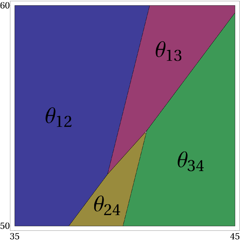
Figure 23: Phase region plot of $\max\{\theta_{12},\theta_{13},\theta_{24},\theta_{34}\}$ for the P-type solution at $t=0$ and with $p_{1}=-2,p_{2}=-1/2,p_{3}=1/4,p_{4}=5/4$, $c_{1}=c_{4}=0$, $c_{2}=-c_{3}=-10$.

Example 4.5.

Here we consider $\tau_{P}$ with $p_{1}+p_{4}=p_{2}+p_{3}$. Writing

$$p_{1}=\frac{1}{2}(q-a-b)\,,\quad p_{2}=\frac{1}{2}(q-a)\,,\quad p_{3}=\frac{1}{2}(q+a)\,,\quad p_{4}=\frac{1}{2}(q+a+b)\,,$$

which real constants $a,b>0$ and $q$, we find

$$x_{12,13} = -q\,y-\frac{1}{4}(a^{2}+3q^{2})\,t+\frac{1}{a}\Big{(}c_{2}-c_{3}-\log(1+2a/b)\Big{)}\,,$$

$$x_{12,24} = -q\,y-\frac{1}{4}[(a+b)^{2}+3q^{2}]\,t+\frac{1}{a+b}\Big{(}c_{1}-c_{4}-\log(1+2a/b)\Big{)}\,,$$

$$x_{12,34} = -q\,y-\frac{1}{4}(a^{2}+ab+b^{2}+3q^{2})\,t+\frac{1}{2a+b}(c_{1}+c_{2}-c_{3}-c_{4})\,,$$

$$x_{13,24} = -q\,y-\frac{1}{4}(3a^{2}+3ab+b^{2}+3q^{2})\,t+\frac{1}{b}(c_{1}-c_{2}+c_{3}-c_{4})\,,$$

$$x_{13,34} = -q\,y-\frac{1}{4}[(a+b)^{2}+3q^{2}]\,t+\frac{1}{a+b}\Big{(}c_{1}-c_{4}+\log(1+2a/b)\Big{)}\,,$$

$$x_{24,34} = -q\,y-\frac{1}{4}(a^{2}+3q^{2})\,t+\frac{1}{a}\Big{(}c_{2}-c_{3}+\log(1+2a/b)\Big{)}\;.$$

Hence all these lines are parallel with slope $-1/q$. The two boundary lines $x=x_{12,13}$ and $x=x_{24,34}$ move with the same speed, and the same holds for $x=x_{12,24}$ and $x=x_{13,34}$. We note that $x_{12,13}<x_{24,34}$ and $x_{12,24}<x_{13,34}$. Furthermore, we find the following coincidence events:

$$x_{13,24}=x_{13,34}=x_{24,34}\quad \quad t=t_{0}-\Delta t=:t_{-}$$

$$x_{12,34}=x_{13,24}\quad \quad t=t_{0}$$ at

$$x_{12,13}=x_{12,24}=x_{13,24}\quad \quad t=t_{0}+\Delta t=:t_{+}\,,$$

where

$$t_{0}=4\frac{a(c_{1}-c_{4})-(a+b)(c_{2}-c_{3})}{ab(a+b)(2a+b)}\,,\qquad\Delta t=\frac{4\log(1+2a/b)}{a(a+b)(2a+b)}>0\;.$$

Since $\theta_{12}-\theta_{13}=\frac{1}{4}ab(a+b)(t-t_{0})-\log(1+2a/b)$ and $\theta_{12}-\theta_{24}=-\frac{1}{4}ab(a+b)(t-t_{0})-\log(1+2a/b)$ on $x=x_{12,34}$, we conclude that this line is never visible. Hence also the event at $t_{0}$ is non-visible. Along $x=x_{12,13}$ we find $\theta_{12}-\theta_{24}=-(q-2p_{1})(q-p_{1}-p_{2})(p_{2}-p_{1})(t-t_{+})$ and $\theta_{12}-\theta_{34}=-(q-2p_{1})(q-p_{1}-p_{2})(p_{2}-p_{1})(t-t_{+})+2\log[(q-p_{2}-p_{1})/(p_{2}-p_{1})]$, which are both positive for $t<t_{+}$, and the first expression is negative for $t>t_{+}$. Hence $x=x_{12,13}$ is visible for $t<t_{+}$ and non-visible for $t>t_{+}$. In the same way we find that $x=x_{13,34}$ is visible for $t<t_{-}$ and non-visible for $t>t_{-}$, $x=x_{12,24}$ is visible for $t>t_{+}$ and non-visible for $t<t_{+}$, $x=x_{24,34}$ is visible for $t>t_{-}$ and non-visible for $t<t_{-}$, and $x=x_{13,24}$ is visible for $t_{-}<t<t_{+}$ and non-visible otherwise. There are no further visible lines. Hence, for $t<t_{-}$ and $t>t_{+}$ there are two visible boundary lines corresponding to two parallel line solitons (oblique to the $x$-axis). But for $t_{-}<t<t_{+}$ there are three parallel visible boundary lines, see also Fig. 24. This means that for $t<t_{-}$ and $t>t_{+}$ only three of the four phases are visible, and all four are visible only for $t_{-}<t<t_{+}$.

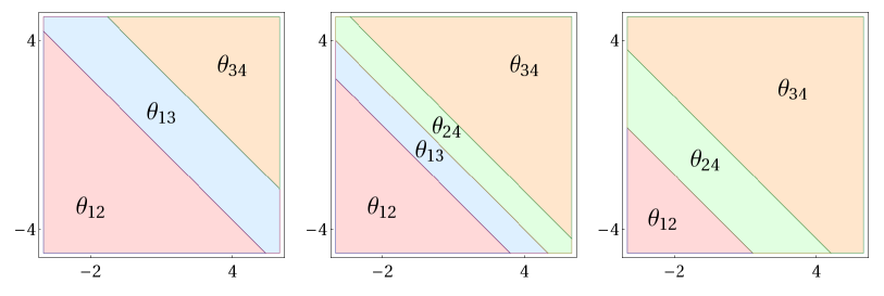
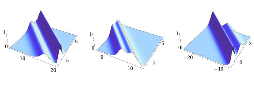
Figure 24: Phase region plot of a solution with two parallel line solitons, as described in Example 4.5, at times $t=-2,0,2$. They exchange a “virtual line soliton”. Here we chose $q=a=1$, $b=1/2$ and $c_{i}=0$, $i=1,\ldots,4$. To the right are plots of the exact solution at $t=-10,0,10$.

The tropical description provides us with an interpretation of the soliton interaction process. For $t<t_{-}$ (left of the three region plots in Fig. 24) the lines $x_{12,13}\simeq x_{23}$ and $x_{13,34}\simeq x_{14}$ represent two line solitons moving from right to left, where the latter is faster than the first. At $t_{-}$ the faster soliton sends off a virtual line soliton (corresponding to $x_{13,24}$) and thereby mutates to $x_{24,34}\simeq x_{23}$, which is a new manifestation of the slower line soliton. At $t_{+}$ the original slower soliton swallows the virtual one and mutates to $x_{12,24}\simeq x_{14}$, which is a new manifestation of the original faster soliton. A generalization of this solution, now with $n$ parallel line solitons, is given by

$$\tau=(e_{1}-(-1)^{n}e_{2n})\wedge(e_{2}-(-1)^{n-1}e_{2n-1})\wedge\cdots\wedge(e_{n-1}-e_{n+2})\wedge(e_{n}+e_{n+1})\,,$$

where $p_{1}<p_{2}<\cdots<p_{2n}$ and $p_{1}+p_{2n}=p_{2}+p_{2n-1}=\cdots=p_{n-1}+p_{n+2}=p_{n}+p_{n+1}$. Moreover, by taking the wedge product of two such functions, we can generate grid-like structures. For example, let

$$\tau=(e_{-6}+e_{-1})\wedge(e_{-5}-e_{-2})\wedge(e_{-4}+e_{-3})\wedge(e_{1}+e_{6})\wedge(e_{2}-e_{5})\wedge(e_{3}+e_{4})\,,$$

where $p_{-6}<p_{-5}<\cdots<p_{-1}<p_{1}<\cdots<p_{6}$, $p_{-6}+p_{-1}=p_{-5}+p_{-2}=p_{-4}+p_{-3}$ and $p_{1}+p_{6}=p_{2}+p_{5}=p_{3}+p_{4}$. Fig. 25 shows a plot of such a solution.

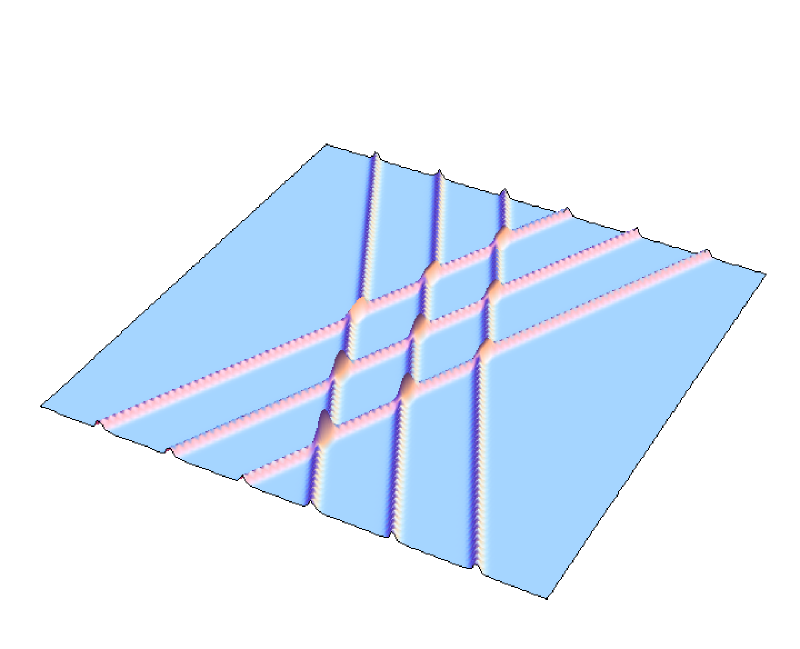
Figure 25: Plot of a grid-like solution at a fixed time, built from two families of parallel line solitons, as described in Example 4.5.

The above results suggest that the line soliton solution is generically obtained as a superimposition of the constituents (i.e. the factors in the wedge product, modulo conversion of negative to positive signs) and in addition with the creation of new line segments of constant length and slope due to the $\log\Delta$ phase shift terms, as in Example 4.3. Typically these new line segments will not be visible in a line soliton plot, with the exception of the extremal cases considered next.

We explore what happens when two neighboring constants, say $p_{i},p_{i+1}$, in the sequence of $p$’s approach each other. Writing $p_{i+1}-p_{i}=e^{-\alpha_{i}}$ and $b_{i}=e^{c_{i+1}-c_{i}}$, we have $e_{i+1}\simeq b_{i}\,e_{i}$ for large positive $\alpha_{i}$. If $i,i+1\in\{k_{1},\ldots,k_{n}\}$, we find

$$\log\Delta(p_{k_{1}},\ldots,p_{k_{n}})\simeq\log\Big{(}\frac{\partial}{\partial p_{i+1}}\Delta(p_{k_{1}},\ldots,p_{k_{n}})\Big{)}_{p_{i+1}=p_{i}}-\alpha_{i}\;.$$

As a consequence, the region dominated by $\theta_{k_{1},\ldots,i,i+1,\ldots,k_{n}}$ disappears in the limit $\alpha_{i}\to\infty$.

If $i+1\in\{k_{1},\ldots,k_{n}\}$, but $i\not\in\{k_{1},\ldots,k_{n}\}$, then

$$\theta_{k_{1}\ldots k_{n}} = \theta_{k_{1}}+\cdots+\theta_{i+1}+\cdots+\theta_{k_{n}}+\log\Delta(p_{k_{1}},\ldots,p_{i+1},\ldots,p_{k_{n}})$$

$$\simeq \theta_{k_{1}}+\cdots+\theta_{i}+\cdots+\theta_{k_{n}}+\log b_{i}+\log\Delta(p_{k_{1}},\ldots,p_{i},\ldots,p_{k_{n}})$$

$$= \theta_{k_{1}\ldots i\ldots k_{n}}+\log b_{i}=:\tilde{\theta}_{k_{1}\ldots i\ldots k_{n}}\;.$$

Hence the $\theta_{k_{1}\ldots i+1\ldots k_{n}}$-region passes into a $\tilde{\theta}_{k_{1}\ldots i\ldots k_{n}}$-region. Boundary lines between regions that do not carry an index $i+1$ remain unchanged.

We conclude that, as $p_{i+1}\to p_{i}$, each region with dominating phase of the form $\theta_{k_{1},\ldots,i,i+1,\ldots,k_{n}}$ is shifted away, the phase regions to its left and to its right meet, a corresponding boundary line is created.

Example 4.6.

We consider regular 2-form solutions with five phases (i.e. $M=4$), $p_{1}<p_{2}<p_{3}<p_{4}<p_{5}$, and limits where two neighboring constants coincide.
(1) $\tau=(e_{1}+e_{2})\wedge(e_{3}+e_{4}+e_{5})$. Setting $p_{3}=p_{2}$, we have $e_{3}=a\,e_{2}$ with a constant $a>0$. Recalling that a constant overall factor of $\tau$ does not change the respective KP soliton solution, after a redefinition of $c_{4}$ and $c_{5}$, and a renumbering, we obtain $\tau^{\prime}=(e_{1}+e_{2})\wedge(e_{2}+e_{3}+e_{4})$. Fig. 26 shows an example for what happens as $p_{3}\to p_{2}$. The phase region associated with this pair is shifted away to infinity in this limit.

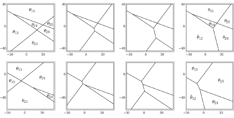
Figure 26: Tropical approximation of an exact solution of the form $\tau=(e_{1}+e_{2})\wedge(e_{3}+e_{4}+e_{5})$, i.e. a superposition of a single line soliton and a Miles resonance, at two different times. From left to right, $p_{3}$ approaches $p_{2}$. In the rightmost plots we have $p_{3}=p_{2}$.

(2) $\tau=(e_{1}+e_{2}-e_{5})\wedge(e_{3}+e_{4})$. Setting $p_{5}=p_{4}$, after a redefinition of $c_{1}$ and $c_{2}$ we end up with $\tau^{\prime}=(e_{1}+e_{2}-e_{4})\wedge(e_{3}+e_{4})$.
(3) $\tau=(e_{1}-e_{5})\wedge(e_{2}+e_{3}+e_{4})$. Setting $p_{5}=p_{4}$, after a redefinition of $c_{1}$ we obtain $\tau^{\prime}=(e_{1}-e_{4})\wedge(e_{2}+e_{3}+e_{4})$.
(4) $\tau=(e_{1}-e_{4}-e_{5})\wedge(e_{2}+e_{3})$. Setting $p_{4}=p_{3}$, redefining $c_{1}$ and $c_{5}$, and finally renaming $p_{5}$ to $p_{4}$, we find $\tau^{\prime}=(e_{1}-e_{3}-e_{4})\wedge(e_{2}+e_{3})$.
Starting with a regular six phase solution, via two limits we obtain a four phase solution:
(5) $\tau=(e_{1}+e_{2}-e_{6})\wedge(e_{3}+e_{4}+e_{5})$. We set $p_{6}=p_{5}$ and $p_{3}=p_{2}$ to obtain $(e_{1}+e_{2}-a\,e_{5})\wedge(b\,e_{2}+e_{4}+e_{5})$. We can achieve $a=1$ with a redefinition of $c_{1}$ and $c_{2}$, or $b=1$ with a redefinition of $c_{4}$ and $c_{5}$, but not both simultaneously. After a renumbering we obtain $\tau^{\prime}=(e_{1}+e_{2}-e_{4})\wedge(a\,e_{2}+e_{3}+e_{4})$, $a>0$. Fig. 27 shows a structure appearing in the tropical approximation that is not present in the full solution. But there are parameter values where the two bounded regions in the left plot in Fig. 27 indeed become visible (cf. Fig. 4 in [10]).

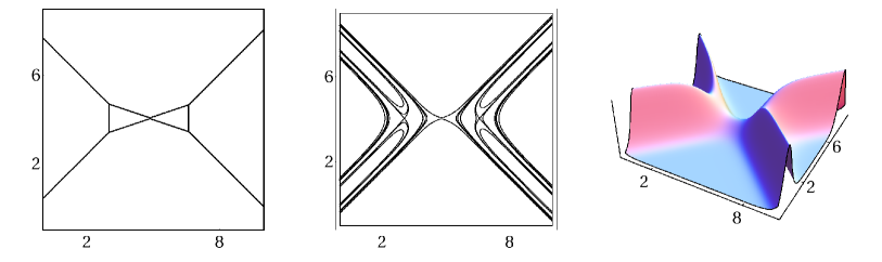
Figure 27: The left plot shows the tropical approximation of a solution of type (5) in Example 4.6 at a fixed time in a region of size comparable with the width of a line soliton. The other plots show the full solution in the same region as a contour plot and a three-dimensional plot over the $xy$-plane.

Together with $\tau_{O}$ and $\tau_{P}$, we have seven types of four-phase 2-form solutions (cf. the seven cases of $(2,2)$-solutions in [19]). Modulo redefinitions of the constants $c_{i}$, $\tau^{\prime}$ in (2) is the dual of that in (1), and also (3) and (4) are related in this way. $\tau_{O},\tau_{P}$ and $\tau^{\prime}$ in (5) are self-dual.

5 Summary of further results and conclusions

For the simplest class of KP-II line soliton solutions, we have shown that the time evolution can be described as a time-ordered sequence of rooted binary trees and that this constitutes a maximal chain in a Tamari lattice.

Moreover, we derived general results (in particular in Appendix Appendix A: Some general results) that allow to compute the data corresponding to transition events (where a rooted binary tree evolves into another). The fact that the soliton solutions extend to solutions of the KP hierarchy plays a crucial role in the derivation of these results.

Tamari lattices are related to quite a number of mathematical structures and our work adds to it by establishing a bridge to an integrable PDE, the KP equation (and moreover its hierarchy). The latter is well-known for other deep connections with various areas of mathematics.

The family of Tamari lattices is actually not the only family of posets (or lattices) showing up in the line soliton classification problem. We already met in section 2 a family where the nodes are the phases $\theta_{i}$ and the edges correspond to critical values of $x$. The underlying polytopes are a triangle ($M=2$), a tetrahedron ($M=3$), and their higher-dimensional analogs ($M>3$). Another family appeared in section 3.1. Its nodes consist of chains of critical $x$-values and the edges correspond to critical $y$-values. The underlying polytopes are a tetragon ($M=3$), a cube ($M=4$), and hypercubes for $M>4$.

According to Figs. 18 and 19 (see also Fig. 14) there is a new lattice of hexagon form. Its six nodes are given by the six classes built from the nine maximal chains of $\mathbb{T}_{4}$ (see Figs. 18 and 19, and also Appendix Appendix C: A symbolic representation of trees with levels, and a relation between permutohedra and Tamari lattices), and its edges correspond to the six critical values of $t^{(4)}$. This lattice is an analog of the pentagon Tamari lattice $\mathbb{T}_{3}$ and belongs to a new family. Its next member is obtained for $M=6$. It has 25 nodes, which consist of classes of maximal chains in $\mathbb{T}_{5}$ (see Appendix Appendix C: A symbolic representation of trees with levels, and a relation between permutohedra and Tamari lattices), and its (directed) edges are again determined by the critical values of $t^{(4)}$, see Fig. 28.

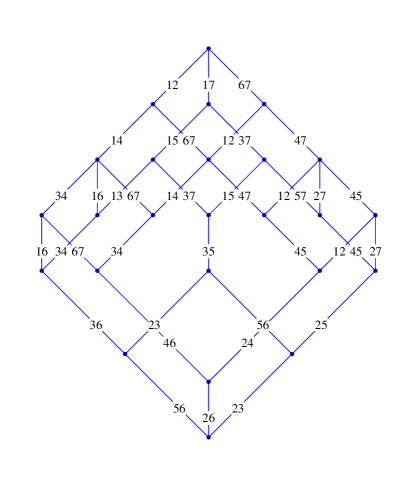
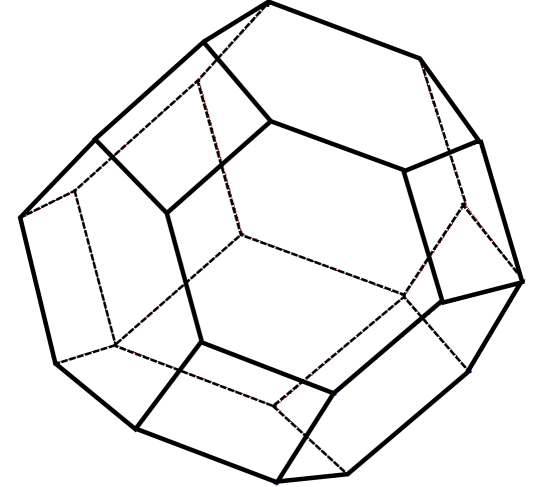
Figure 28: The left figure shows a new lattice. Its nodes are classes of maximal chains in $\mathbb{T}_{5}$ and the edges correspond to critical values of $t^{(4)}$. A two-digit number stands for its complement in $1234567$. The right figure represents this lattice as a polyhedron. It has 25 nodes, 39 edges and 16 faces, and it consists of seven hexagons and nine tetragons.

Moreover, we expect a hierarchy of families of lattices. We already mentioned the two families associated with the critical values of $x$ and $y$. The Tamari lattices correspond to the critical values of $t=t^{(3)}$, the next family is associated with the critical values of $t^{(4)}$. More generally, there is a family associated with the critical values of $t^{(n)}$, $n\in\mathbb{N}$. Comparison with the algebra of oriented simplexes formulated in [45] (see also [46]) in terms of higher-dimensional categories shows striking relations which should be further elaborated. An exploration of more general classes of line solitons might exhibit relations with other posets (or lattices) and polytopes.

In this work we solved the classification problem for the simplest class of KP-II line soliton solutions, corresponding to rooted trees. Our classification rests upon the exploration of events where phases coincide. At such an event the tree that describes the line soliton configuration changes its form. A finer description is obtained by taking also events into account at which a transition between two trees with levels (associated with the same rooted binary tree) takes place. Our exposition made contact with such a refinement at various places. A nice example is the “missing face” in the cube poset in Fig. 10. We elaborated this refinement in Appendix Appendix B: A finer classification in terms of trees with levels and explained in Appendix Appendix C: A symbolic representation of trees with levels, and a relation between permutohedra and Tamari lattices how it lifts the Tamari lattices (or associahedra) to permutohedra.

At first sight the classification for the simple class of line soliton solutions appears to be only a small step towards the classification of the whole set of line soliton solutions, which exhibit a much more complicated behavior. But this is not quite so, as outlined in section 4. Any line soliton solution can be written as a (suitably defined) exterior product of $\tau$-functions from the simple class. Generically such a product corresponds to superimposing the soliton graphs associated with the constituents. Since the interaction is local, there can only be a change in a neighborhood of a point where a soliton branch of one constituent meets a branch of another. At such a point a new line soliton segment (due to a phase shift) is created and its length does not depend on time and not on the constants $c_{i}$, but only on the values of the constants $p_{i}$. For generic parameter values, this effect is hardly visible. It becomes significant, however, in cases where some of the (a priori assumed to be different) constants $p_{i}$ coincide. These are the more complicated cases which should still be explored in more detail.

We expect that our tropical approximations of KP line soliton solutions have a place in the tropical (totally positive) Grassmannian [47, 48]. For other approaches to the KP line soliton classification problem we refer in particular to the review [19] and the references therein.

Finally, we would like to stress that the tropical approximation allows to zoom into the interaction structure of solitons and enriches it with an underlying quantum particle-like picture (see Example 4.5). We expect that this tropical approach will also be useful in case of other (in particular soliton) equations.

Appendix A: Some general results

A.1 Preparations

The phases $\theta_{k}$ appearing in the expression for the function $\tau$ have the form

$$\theta_{k}=\sum_{r=1}^{n-1}p_{k}^{r}\,t^{(r)}+c_{k}\,,$$

where $p_{k},c_{k}\in\mathbb{R}$ and $t^{(r)}$, $r=1,\ldots,n-1$, are real variables. The constants $p_{i}$ are assumed to be pairwise different. In previous sections we wrote $t^{(1)}=x,t^{(2)}=y,t^{(3)}=t$. In order to find the values of $t^{(r)}$ for which $\theta_{k_{1}}=\theta_{k_{2}}=\cdots=\theta_{k_{n}}=:-t^{(0)}$, we have to solve the linear system

$$p_{k_{i}}^{n-1}\,t^{(n-1)}+p_{k_{i}}^{n-2}\,t^{(n-2)}+\cdots+p_{k_{i}}\,t^{(1)}+t^{(0)}=-c_{k_{i}}\qquad\quad i=1,\ldots,n\,,$$

which is done with the help of Cramer’s rule. In particular, for $t^{(n-1)}$ we obtain the solution

$$t^{(n-1)}_{k_{1}\ldots k_{n}}=-c_{k_{1}\ldots k_{n}}\,,$$ (A.1)

where

$$c_{k_{1}\ldots k_{n}}=\frac{\kappa(p_{k_{1}},\ldots,p_{k_{n}})}{\Delta(p_{k_{1}},\ldots,p_{k_{n}})}$$ (A.2)

with the Vandermonde determinant

$$\Delta(p_{k_{1}},\ldots,p_{k_{n}})=\left|\begin{array}[]{cccc}1&p_{k_{1}}&\cdots&p_{k_{1}}^{n-1}\\ 1&p_{k_{2}}&\cdots&p_{k_{2}}^{n-1}\\ \vdots&\vdots&&\vdots\\ 1&p_{k_{n}}&\cdots&p_{k_{n}}^{n-1}\end{array}\right|=\prod_{1\leq i<j\leq n}(p_{k_{j}}-p_{k_{i}})$$ (A.7)

and

$$\kappa(p_{k_{1}},\ldots,p_{k_{n}}) = \left|\begin{array}[]{ccccc}1&p_{k_{1}}&\cdots&p_{k_{1}}^{n-2}&c_{k_{1}}\\ 1&p_{k_{2}}&\cdots&p_{k_{2}}^{n-2}&c_{k_{2}}\\ \vdots&\vdots&&\vdots&\vdots\\ 1&p_{k_{n}}&\cdots&p_{k_{n}}^{n-2}&c_{k_{n}}\end{array}\right|=(-1)^{n-1}\sum_{i=1}^{n}(-1)^{i-1}c_{k_{i}}\left|\begin{array}[]{cccc}1&p_{k_{1}}&\cdots&p_{k_{1}}^{n-2}\\ \vdots&\vdots&&\vdots\\ 1&p_{k_{i-1}}&\cdots&p_{k_{i-1}}^{n-2}\\ 1&p_{k_{i+1}}&\cdots&p_{k_{i+1}}^{n-2}\\ \vdots&\vdots&&\vdots\\ 1&p_{k_{n}}&\cdots&p_{k_{n}}^{n-2}\end{array}\right|$$

$$= \sum_{i=1}^{n}(-1)^{n-i}c_{k_{i}}\,\Delta(p_{k_{1}},\ldots,\widehat{p_{k_{i}}},\ldots,p_{k_{n}})\;.$$

Here a hat indicates an omission. Now (A.2) implies

$$c_{k_{1}\ldots k_{n}}=\sum_{i=1}^{n}\frac{c_{k_{i}}}{(p_{k_{i}}-p_{k_{1}})\cdots(p_{k_{i}}-p_{k_{i-1}})(p_{k_{i}}-p_{k_{i+1}})\cdots(p_{k_{i}}-p_{k_{n}})}\;.$$ (A.9)

Proposition A.1.

$$c_{k_{1}\ldots k_{n+1}}=\frac{c_{k_{1}\ldots\widehat{k_{i}}\ldots k_{n+1}}-c_{k_{1}\ldots\widehat{k_{j}}\ldots k_{n+1}}}{p_{k_{j}}-p_{k_{i}}}\qquad\quad(i\neq j)\;.$$

Proof: Since $c_{k_{1}\ldots k_{n}}$ is totally symmetric, it suffices to prove the formula for $i=1$ and $j=n+1$. Using (A.9) we have

$$c_{k_{2}\ldots k_{n+1}}-c_{k_{1}\ldots k_{n}}=\frac{c_{k_{n+1}}}{(p_{k_{n+1}}-p_{k_{2}})\cdots(p_{k_{n+1}}-p_{k_{n}})}-\frac{c_{k_{1}}}{(p_{k_{1}}-p_{k_{2}})\cdots(p_{k_{1}}-p_{k_{n}})}$$

$$+\sum_{r=2}^{n}\Big{(}\frac{1}{(p_{k_{r}}-p_{k_{n+1}})}-\frac{1}{(p_{k_{r}}-p_{k_{1}})}\Big{)}\frac{c_{k_{r}}}{(p_{k_{r}}-p_{k_{2}})\cdots(p_{k_{r}}-p_{k_{r-1}})(p_{k_{r}}-p_{k_{r+1}})\cdots(p_{k_{r}}-p_{k_{n}})}\,,$$

hence

$$\frac{c_{k_{2}\ldots k_{n+1}}-c_{k_{1}\ldots k_{n}}}{p_{k_{n+1}}-p_{k_{1}}}=\frac{c_{k_{1}}}{(p_{k_{1}}-p_{k_{2}})\cdots(p_{k_{1}}-p_{k_{n+1}})}+\frac{c_{k_{n+1}}}{(p_{k_{n+1}}-p_{k_{1}})\cdots(p_{k_{n+1}}-p_{k_{n}})}$$

$$+\sum_{r=2}^{n}\frac{c_{k_{r}}}{(p_{k_{r}}-p_{k_{1}})\cdots(p_{k_{r}}-p_{k_{r-1}})(p_{k_{r}}-p_{k_{r+1}})\cdots(p_{k_{r}}-p_{k_{n+1}})}=c_{k_{1}\ldots k_{n+1}}\;.$$

$\square$

Proposition A.2.

The substitution $c_{k}\mapsto c_{k}+p_{k}^{r}\,t^{(r)}$, with a variable $t^{(r)}$, has the following effect,

$$c_{k_{1}\ldots k_{n}}\mapsto c_{k_{1}\ldots k_{n}}+h_{r-n+1}(p_{k_{1}},\ldots,p_{k_{n}})\,t^{(r)}\,,$$

where $h_{m}$, $m=1,2,\ldots$, are the complete symmetric polynomials, and $h_{m}=0$ if $m<0$, $h_{0}=1$.

Proof: By linearity of the determinant, the substitution effects $\kappa(p_{k_{1}},\ldots,p_{k_{n}})$ as follows,

$$\kappa(p_{k_{1}},\ldots,p_{k_{n}})\mapsto\kappa(p_{k_{1}},\ldots,p_{k_{n}})+\left|\begin{array}[]{ccccc}1&p_{k_{1}}&\cdots&p_{k_{1}}^{n-2}&p_{k_{1}}^{r}\\ \vdots&\vdots&&\vdots&\vdots\\ 1&p_{k_{n}}&\cdots&p_{k_{n}}^{n-2}&p_{k_{n}}^{r}\end{array}\right|\,t^{(r)}\;.$$

The latter determinant equals $h_{r-n+1}(p_{k_{1}},\ldots,p_{k_{n}})\,\Delta(p_{k_{1}},\ldots,p_{k_{n}})$ (see e.g. [49]). Now the assertion follows from the expression (A.2) for $c_{k_{1}\ldots k_{n}}$. $\square$

A redefinition $c_{k}\mapsto c_{k}+\sum_{r=n}^{N}p_{k}^{r}\,t^{(r)}$ changes the expression for the phases to

$$\theta_{k}=\sum_{r=1}^{N}p_{k}^{r}\,t^{(r)}+c_{k}\,,$$

and, by application of the last proposition to (A.1), the critical value for the $n$-phase coincidence $\theta_{k_{1}}=\theta_{k_{2}}=\cdots=\theta_{k_{n}}$ now reads

$$t^{(n-1)}_{k_{1}\ldots k_{n}}=-\sum_{r=1}^{N+1-n}h_{r}(p_{k_{1}},\ldots,p_{k_{n}})\,t^{(n+r-1)}-c_{k_{1}\ldots k_{n}}\,,$$ (A.11)

where $n=2,3,\ldots,N+1$. In particular, $t^{(N)}_{k_{1}\ldots k_{N+1}}=-c_{k_{1}\ldots k_{N+1}}$. (A.11) also makes sense for $n=1$, where $\theta_{k}=-t^{(0)}_{k}$. The following proposition presents identities that have the same form irrespective of the value of $N$, i.e. their form is not affected by the redefinitions expressed in the last proposition. Of course, the ingredients (A.11) do depend on $N$.

Proposition A.3.

For $n=1,\ldots,N+1$ we have

$$t^{(n-1)}_{k_{1}\ldots\widehat{k_{i}}\ldots k_{n+1}}-t^{(n-1)}_{k_{1}\ldots\widehat{k_{j}}\ldots k_{n+1}}=(p_{k_{i}}-p_{k_{j}})(t^{(n)}-t^{(n)}_{k_{1}\ldots k_{n+1}})\qquad\qquad i,j=1,\ldots,n+1\;.$$ (A.12)

Proof: Using (A.11) for fixed $N$, and Proposition A.1, we obtain

$$t^{(n-1)}_{k_{1}\ldots\widehat{k_{i}}\ldots k_{n+1}}-t^{(n-1)}_{k_{1}\ldots\widehat{k_{j}}\ldots k_{n+1}}=(p_{k_{i}}-p_{k_{j}})\,c_{k_{1}\ldots k_{n+1}}$$

$$+\sum_{r=1}^{N+1-n}\Big{(}h_{r}(p_{k_{1}},\ldots,\widehat{p_{k_{j}}},\ldots,p_{k_{n+1}})-h_{r}(p_{k_{1}},\ldots,\widehat{p_{k_{i}}},\ldots,p_{k_{n+1}})\Big{)}\,t^{(n+r-1)}\;.$$

Eliminating $c_{k_{1}\ldots k_{n+1}}$ with the help of (A.11) (with $n$ replaced by $n+1$), we obtain

$$t^{(n-1)}_{k_{1}\ldots\widehat{k_{i}}\ldots k_{n+1}}-t^{(n-1)}_{k_{1}\ldots\widehat{k_{j}}\ldots k_{n+1}}=\underbrace{[h_{1}(p_{k_{1}},\ldots,\widehat{p_{k_{j}}},\ldots,p_{k_{n+1}})-h_{1}(p_{k_{1}},\ldots,\widehat{p_{k_{i}}},\ldots,p_{k_{n+1}})]}_{\mbox{$=p_{k_{i}}-p_{k_{j}}$}}\,t^{(n)}$$

$$-(p_{k_{i}}-p_{k_{j}})\,t^{(n)}_{k_{1}\ldots k_{n+1}}+\sum_{r=1}^{N+1-r}\Big{(}h_{r}(p_{k_{1}},\ldots,\widehat{p_{k_{j}}},\ldots,p_{k_{n+1}})-h_{r}(p_{k_{1}},\ldots,\widehat{p_{k_{i}}},\ldots,p_{k_{n+1}})$$

$$-(p_{k_{i}}-p_{k_{j}})\,h_{r-1}(p_{k_{1}},\ldots,p_{k_{n+1}})\Big{)}\,t^{(n+r-1)}\;.$$

But the last sum vanishes as a consequence of the identities

$$h_{r}(p_{k_{1}},\ldots,\widehat{p_{k_{j}}},\ldots,p_{k_{n+1}})-h_{r}(p_{k_{1}},\ldots,\widehat{p_{k_{i}}},\ldots,p_{k_{n+1}})=(p_{k_{i}}-p_{k_{j}})\,h_{r-1}(p_{k_{1}},\ldots,p_{k_{n+1}})\;.$$

$\square$

A.2 Main results

For fixed $M$, we have $M+1$ phases

$$\theta_{i}=\sum_{r=1}^{M}p_{i}^{r}\,t^{(r)}+c_{i}\qquad\quad i=1,\ldots,M+1\;.$$

In the following we regard the variables $t^{(r)}$, $r=1,\ldots,M$, as Cartesian coordinates on $\mathbb{R}^{M}$. The region in $\mathbb{R}^{M}$ where $\theta_{i}$ dominates is given by

$$\mathcal{U}_{i}=\{\mathbf{t}\in\mathbb{R}^{M}\,|\,\max\{\theta_{1}(\mathbf{t}),\ldots,\theta_{M+1}(\mathbf{t})\}=\theta_{i}(\mathbf{t})\}\;.$$

Associated with any set $\{k_{1},\ldots,k_{n+1}\}\subset\{1,\ldots,M+1\}$, $n>0$, there is a critical plane,

$$\mathcal{P}_{k_{1}\ldots k_{n+1}}=\{\mathbf{t}\in\mathbb{R}^{M}\,|\,\theta_{k_{1}}(\mathbf{t})=\cdots=\theta_{k_{n+1}}(\mathbf{t})\}\,,$$

which is an affine plane of dimension $M-n$. Since the $p_{i}$ are pairwise different, no pair of hyperplanes $\mathcal{P}_{ij}$, $1\leq i<j\leq M+1$, can be parallel. In particular, they cannot coincide and thus $\mathcal{U}_{i}\neq\emptyset$, $i=1,\ldots,M+1$. We also note that $\bigcup_{1\leq i\leq M+1}\mathcal{U}_{i}=\mathbb{R}^{M}$. Some obvious relations are

$$\mathcal{P}_{k_{1}\ldots k_{n+1}}\subset\mathcal{P}_{k_{1}\ldots k_{m+1}}\qquad\mbox{for}\qquad m<n\,,$$

and

$$\mathcal{P}_{k_{1}\ldots k_{n+1}}=\mathcal{P}_{k_{1}\ldots\widehat{k_{r}}\ldots k_{n+1}}\cap\mathcal{P}_{k_{1}\ldots\widehat{k_{s}}\ldots k_{n+1}}\qquad\mbox{for}\qquad r\neq s\,,$$

where a hat again indicates an omission, hence also

$$\mathcal{P}_{k_{1}\ldots k_{n+1}}=\bigcap_{r=1}^{n+1}\mathcal{P}_{k_{1}\ldots\widehat{k_{r}}\ldots k_{n+1}}\;.$$

We can use $t^{(n+1)},\ldots,t^{(M)}$ as coordinates on $\mathcal{P}_{k_{1}\ldots k_{n+1}}$, since on this subset of $\mathbb{R}^{M}$ the remaining coordinates are fixed as solutions of the system $\theta_{k_{1}}=\cdots=\theta_{k_{n+1}}=:-t^{(0)}$, i.e.

$$\sum_{r=0}^{n}p_{k_{j}}^{r}\,t^{(r)}=-c_{k_{j}}-\sum_{r=n+1}^{M}p_{k_{j}}^{r}\,t^{(r)}\qquad\quad j=1,\ldots,n+1\;.$$

We solve this system for $t^{(r)}$, $r=1,\ldots,n$, and denote the solutions as $t^{(r)}_{k_{1}\ldots k_{n+1}}(t^{(n+1)},\ldots,t^{(M)})$, $r=1,\ldots,n$. They depend linearly on the parameters $c_{i}$. For the highest we already found

$$t^{(n)}_{k_{1}\ldots k_{n+1}}(t^{(n+1)},\ldots,t^{(M)})=-\sum_{r=1}^{M-n}h_{r}(p_{k_{1}},\ldots,p_{k_{n+1}})\,t^{(n+r)}-c_{k_{1}\ldots k_{n+1}}\,,$$

which is totally symmetric in the lower indices. These are called critical values of $t^{(n)}$. The values of $t^{(r)}_{k_{1}\ldots k_{n+1}}(t^{(n+1)},\ldots,t^{(M)})$, $r=1,\ldots,n-1$, are then determined iteratively as functions of $t^{(n+1)},\ldots,t^{(M)}$. Hence the points of $\mathcal{P}_{k_{1}\ldots k_{n+1}}$ are given by

$$\mathbf{t}_{k_{1}\ldots k_{n+1}}(t^{(n+1)},\ldots,t^{(M)}):=\mathbf{t}(t^{(1)}_{k_{1}\ldots k_{n+1}},\ldots,t^{(n)}_{k_{1}\ldots k_{n+1}},t^{(n+1)},\ldots,t^{(M)})\,,$$

where we suppressed the arguments of $t^{(r)}_{k_{1}\ldots k_{n+1}}$.

Proposition A.4.

Let $\{k_{1},\ldots,k_{n+1}\}\subset\{1,\ldots,M+1\}$ and $p_{k_{i}}<p_{k_{j}}$. Then we have

$$t^{(n-1)}_{k_{1}\ldots\widehat{k_{j}}\ldots k_{n+1}}\lessgtr t^{(n-1)}_{k_{1}\ldots\widehat{k_{i}}\ldots k_{n+1}}\qquad\mbox{for}\qquad t^{(n)}\lessgtr t^{(n)}_{k_{1}\ldots k_{n+1}}\;.$$

Proof: This is an immediate consequence of (A.12). $\square$

Proposition A.5.

Let $\{k_{1},\ldots,k_{n+1}\}\subset\{1,\ldots,M+1\}$. Then

$$\theta_{k_{1}}-\theta_{k_{n+1}}=-\sum_{r=1}^{n}\Big{(}\prod_{j=1}^{r}(p_{k_{n+1}}-p_{k_{j}})\Big{)}\,(t^{(r)}-t^{(r)}_{k_{1}\ldots k_{r+1}})\;.$$ (A.13)

Proof: (A.12) with $n=1$ reads

$$\theta_{k_{1}}-\theta_{k_{2}}=-(p_{k_{2}}-p_{k_{1}})(x-x_{k_{1}k_{2}})\,,$$

which is the above formula for $n=1$. Assuming that the assertion holds for $n$, we can apply it with $\{k_{1},\ldots,k_{n},k_{n+2}\}$ to obtain

$$\theta_{k_{1}}-\theta_{k_{n+2}} = -\sum_{r=1}^{n-1}\Big{(}\prod_{j=1}^{r}(p_{k_{n+2}}-p_{k_{j}})\Big{)}\,(t^{(r)}-t^{(r)}_{k_{1}\ldots k_{r+1}})$$

$$-\Big{(}\prod_{j=1}^{n}(p_{k_{n+2}}-p_{k_{j}})\Big{)}\,(t^{(n)}-t^{(n)}_{k_{1}\ldots k_{n+1}}+t^{(n)}_{k_{1}\ldots k_{n+1}}-t^{(n)}_{k_{1}\ldots k_{n}k_{n+2}})$$

$$= -\sum_{r=1}^{n}\Big{(}\prod_{j=1}^{r}(p_{k_{n+2}}-p_{k_{j}})\Big{)}\,(t^{(r)}-t^{(r)}_{k_{1}\ldots k_{r+1}})$$

$$-\Big{(}\prod_{j=1}^{n}(p_{k_{n+2}}-p_{k_{j}})\Big{)}\,(t^{(n)}_{k_{1}\ldots k_{n+1}}-t^{(n)}_{k_{1}\ldots k_{n}k_{n+2}})\;.$$

Using (A.12) in the last factor, this becomes the asserted formula for $n+1$, which thus completes the induction step. $\square$

Corollary A.6.

Let $\{k_{1},\ldots,k_{n+1}\}\subset\{1,\ldots,M+1\}$. On $\mathcal{P}_{k_{1}\ldots k_{n}}$, we have

$$\theta_{k_{1}}-\theta_{k_{n+1}}=-(p_{k_{n+1}}-p_{k_{1}})(p_{k_{n+1}}-p_{k_{2}})\cdots(p_{k_{n+1}}-p_{k_{n}})(t^{(n)}-t^{(n)}_{k_{1}\ldots k_{n+1}})\;.$$ (A.14)

$\square$

A point $\mathbf{t}_{0}\in\mathcal{P}_{k_{1}\ldots k_{n+1}}$ will be called non-visible if there is an $m\not\in\{k_{1},\ldots,k_{n+1}\}$ such that $\theta_{m}(\mathbf{t}_{0})>\theta_{k_{1}}(\mathbf{t}_{0})$. Otherwise it will be called visible. In previous sections we considered the projection into the $xy$-plane, $P_{k_{1}\ldots k_{n+1}}(t^{(n+1)},\ldots,t^{(M)})$, of a point $\mathbf{t}_{k_{1}\ldots k_{n+1}}(t^{(n+1)},\ldots,t^{(M)})\in\mathcal{P}_{k_{1}\ldots k_{n+1}}$. Our previous notion of visibility of $P_{k_{1}\ldots k_{n+1}}(t^{(n+1)},\ldots,t^{(M)})$, which means ordinary visibility in a plot of $\max\{\theta_{1},\ldots,\theta_{M+1}\}$, is in fact equivalent to visibility of the latter point in $\mathbb{R}^{M}$. In the following, $\lceil n/2\rceil$ denotes the smallest integer greater than or equal to $n/2$, and $\lfloor n/2\rfloor$ the largest integer smaller than or equal to $n/2$.

Proposition A.7.

For $n=1,2,\ldots$, let $\{k_{1},\ldots,k_{n+1}\}\subset\{1,\ldots,M+1\}$, $p_{k_{1}}<p_{k_{2}}<\cdots<p_{k_{n+1}}$, and $t^{(n+1)}_{0},\ldots,t^{(M)}_{0}\in\mathbb{R}$. The following half-lines are non-visible:
(1) $\{\mathbf{t}_{k_{1}\ldots\,\widehat{k_{n-2r}}\,\ldots k_{n+1}}(t^{(n)},t^{(n+1)}_{0},\ldots,t^{(M)}_{0})\,|\,t^{(n)}<t^{(n)}_{k_{1}\ldots k_{n+1}}\}\subset\mathcal{P}_{k_{1}\ldots\,\widehat{k_{n-2r}}\,\ldots k_{n+1}}$, $r=0,\ldots,\lceil n/2\rceil-1$,
(2) $\{\mathbf{t}_{k_{1}\ldots\,\widehat{k_{n+1-2r}}\,\ldots k_{n+1}}(t^{(n)},t^{(n+1)}_{0},\ldots,t^{(M)}_{0})\,|\,t^{(n)}>t^{(n)}_{k_{1}\ldots k_{n+1}}\}\subset\mathcal{P}_{k_{1}\ldots\,\widehat{k_{n+1-2r}}\,\ldots k_{n+1}}$, $r=0,\ldots,\lfloor n/2\rfloor$.
Here $t^{(n)}_{k_{1}\ldots k_{n+1}}$ stands for $t^{(n)}_{k_{1}\ldots k_{n+1}}(t^{(n+1)}_{0},\ldots,t^{(M)}_{0})$.

Proof: On $\mathcal{P}_{k_{1}\ldots\widehat{k_{m}}\ldots k_{n}}$, (A.14) can be written in the form

$$\theta_{k_{1}}-\theta_{k_{m}}=-\Big{(}\prod_{j=1,\ldots,n+1\atop j\neq m}(p_{k_{m}}-p_{k_{j}})\Big{)}\,(t^{(n)}-t^{(n)}_{k_{1}\ldots k_{n+1}})\qquad\quad m=2,\ldots,n+1\;.$$

We actually consider this equation on $\mathcal{P}_{k_{1}\ldots\widehat{k_{m}}\ldots k_{n}}\cap\mathcal{E}$, where $\mathcal{E}$ is the plane in $\mathbb{R}^{M}$ determined by fixing the values of $t^{(n+1)},\ldots,t^{(M)}$ to $t^{(n+1)}_{0},\ldots,t^{(M)}_{0}$. As a consequence of our assumption $p_{k_{1}}<\cdots<p_{k_{n+1}}$, for $m=n+1$ the above expression is negative if $t^{(n)}>t^{(n)}_{k_{1}\ldots k_{n+1}}$, hence $\mathcal{P}_{k_{1}\ldots k_{n}}\cap\mathcal{E}$ is then non-visible. For $m=n$ the expression is negative if $t^{(n)}<t^{(n)}_{k_{1}\ldots k_{n+1}}$, hence $\mathcal{P}_{k_{1}\ldots k_{n-1}k_{n+1}}\cap\mathcal{E}$ is then non-visible. For $m=n-1$, the expression is negative if $t^{(n)}>t^{(n)}_{k_{1}\ldots k_{n+1}}$, hence $\mathcal{P}_{k_{1}\ldots k_{n-2}k_{n}k_{n+1}}\cap\mathcal{E}$ is then non-visible. This argument can be continued as long as $m>1$. On the remaining critical plane $\mathcal{P}_{k_{2}\ldots k_{n+1}}$, which appears in case (1) for odd $n$ and in case (2) for even $n$, we can write the above equation as

$$\theta_{k_{n+1}}-\theta_{k_{1}}=(-1)^{n+1}\Big{(}\prod_{j=2,\ldots,n+1}(p_{k_{j}}-p_{k_{1}})\Big{)}\,(t^{(n)}-t^{(n)}_{k_{1}\ldots k_{n+1}})\;.$$

This is negative if either $n$ is odd and $t^{(n)}<t^{(n)}_{k_{1}\ldots k_{n+1}}$, or if $n$ is even and $t^{(n)}>t^{(n)}_{k_{1}\ldots k_{n+1}}$. As a consequence, $\mathcal{P}_{k_{2}\ldots k_{n+1}}\cap\mathcal{E}$ is then non-visible. $\square$

We note that the set of critical planes in part 1 and part 2 of Proposition A.7 are complementary. In the following we call a critical point $\mathbf{t}_{0}\in\mathcal{P}_{k_{1}\ldots k_{n+1}}$ generic if it is not also a higher order critical point, i.e. if $\mathbf{t}_{0}\not\in\mathcal{P}_{k_{1}\ldots k_{n+2}}$ with any $k_{n+2}\not\in\{k_{1},\ldots,k_{n+1}\}$.

Proposition A.8.

Let $\{k_{1},\ldots,k_{n+1}\}\subset\{1,\ldots,M+1\}$ and $p_{k_{1}}<p_{k_{2}}<\cdots<p_{k_{n+1}}$. Let $\alpha,\beta$ be such that in the open interval $(\alpha,t^{(n)}_{k_{1}\ldots k_{n+1}})$, respectively $(t^{(n)}_{k_{1}\ldots k_{n+1}},\beta)$, there is no critical value of $t^{(n)}$ corresponding to a visible critical point. If $\mathbf{t}_{k_{1}\ldots k_{n+1}}(t^{(n+1)}_{0},\ldots,t^{(M)}_{0})$ is generic and visible, then the following line segments are visible:
(1) $\{\mathbf{t}_{k_{1}\ldots\,\widehat{k_{n+1-2r}}\,\ldots k_{n+1}}(t^{(n)},t^{(n+1)}_{0},\ldots,t^{(M)}_{0})\,|\,\alpha\leq t^{(n)}\leq t^{(n)}_{k_{1}\ldots k_{n+1}}\}\subset\mathcal{P}_{k_{1}\ldots\,\widehat{k_{n+1-2r}}\,\ldots k_{n+1}}$, where $r=0,\ldots,\lfloor n/2\rfloor$,
(2) $\{\mathbf{t}_{k_{1}\ldots\,\widehat{k_{n-2r}}\,\ldots k_{n+1}}(t^{(n)},t^{(n+1)}_{0},\ldots,t^{(M)}_{0})\,|\,t^{(n)}_{k_{1}\ldots k_{n+1}}\leq t^{(n)}\leq\beta\}\subset\mathcal{P}_{k_{1}\ldots\,\widehat{k_{n-2r}}\,\ldots k_{n+1}}$, where $r=0,\ldots,\lceil n/2\rceil-1$.
Here we set $t^{(n)}_{k_{1}\ldots k_{n+1}}=t^{(n)}_{k_{1}\ldots k_{n+1}}(t^{(n+1)}_{0},\ldots,t^{(M)}_{0})$.

Proof: In the following we use $\mathcal{E}$ as defined in the proof of Proposition A.7. Since we assume $\mathbf{t}_{0}:=\mathbf{t}_{k_{1}\ldots k_{n+1}}(t^{(n+1)}_{0},\ldots,t^{(M)}_{0})\in\mathcal{P}_{k_{1}\ldots k_{n+1}}$ to be visible, at $\mathbf{t}_{0}$ the phases $\theta_{k_{1}},\ldots,\theta_{k_{n+1}}$ coincide and dominate. Since $\mathbf{t}_{0}$ is assumed to be generic, there is a neighborhood of $\mathbf{t}_{0}$ in $\mathcal{E}$ which is covered by the polyhedral cones $\mathcal{U}_{k_{j}}\cap\mathcal{E}$, $j=1,\ldots,n+1$. Since each line $\mathcal{P}_{k_{1}\ldots\widehat{k_{n-2r}}\ldots k_{n+1}}\cap\mathcal{E}$, $r\in\{1,\ldots,n+1\}$, contains $\mathbf{t}_{0}$, it follows that its visible part $\mathcal{P}_{k_{1}\ldots\widehat{k_{n-2r}}\ldots k_{n+1}}\cap\mathcal{E}\cap\mathcal{U}_{k_{1}}\cap\cdots\cap\mathcal{U}_{k_{r-1}}\cap\mathcal{U}_{k_{r+1}}\cap\cdots\cap\mathcal{U}_{k_{n+1}}$ extends in the direction complementary to that in Proposition A.7, either indefinitely or up to a point of $\mathcal{E}$ where it meets $\mathcal{U}_{m}$ with some $m\not\in\{k_{1},\ldots,k_{n+1}\}$. We only need to consider the latter case further. Then $\{\mathbf{t}_{1}\}:=\mathcal{U}_{k_{1}}\cap\cdots\cap\mathcal{U}_{k_{r-1}}\cap\mathcal{U}_{k_{r+1}}\cap\cdots\cap\mathcal{U}_{k_{n+1}}\cap\mathcal{U}_{m}\cap\mathcal{E}$ is a visible point in $\mathcal{P}_{k_{1}\ldots\widehat{k_{n-2r}}\ldots k_{n+1}m}\cap\mathcal{E}$. Since the line between $\mathbf{t}_{0}$ and $\mathbf{t}_{1}$ is visible, it cannot be part of the non-visible half-line determined by Proposition A.7 applied to $\mathbf{t}_{1}$. $\square$

The following proposition shows that the existence of a visible critical point requires the existence of a visible critical point one level higher.

Proposition A.9.

Let $n\leq M$ and $t^{(r)}_{0}\in\mathbb{R}$, $r=n,\ldots,M$. If all points $\mathbf{t}_{k_{1}\ldots k_{n+1}}(t^{(n+1)}_{0},\ldots,t^{(M)}_{0})$, where $\{k_{1},\ldots,k_{n+1}\}\supset\{l_{1},\ldots,l_{n}\}$, are non-visible, then the line $\{\mathbf{t}_{l_{1}\ldots l_{n}}(t^{(n)},t^{(n+1)}_{0},\ldots,t^{(M)}_{0})\,|\,t^{(n)}\in\mathbb{R}\}$, is non-visible.

Proof: Let $\mathcal{E}$ again denote the set $\{\mathbf{t}\in\mathbb{R}^{M}\,|\,t^{(n+1)}=t^{(n+1)}_{0},\ldots,t^{(M)}=t^{(M)}_{0}\}$ and let $\mathbf{t}_{0}\in\mathcal{P}_{l_{1}\ldots l_{n}}\cap\mathcal{E}$ be visible. Since $n\leq M$, a critical point exists one level higher, given by $\{\mathbf{t}_{1}\}=\mathcal{P}_{k_{1}\ldots k_{n+1}}\cap\mathcal{E}$ with some $k_{1},\ldots,k_{n+1}$ such that $\{l_{1},\ldots,l_{n}\}\subset\{k_{1},\ldots,k_{n+1}\}$. If this point is visible, the proposition holds. If $\mathbf{t}_{1}$ is non-visible, then $\mathbf{t}_{1}\in\mathcal{U}_{m}\cap\mathcal{E}$ with some $m\not\in\{k_{1},\ldots,k_{n+1}\}$. Clearly, it cannot coincide with $\mathbf{t}_{0}$. By continuity, on the line segment between $\mathbf{t}_{0}$ and $\mathbf{t}_{1}$ a visible critical point then exists, which is $\mathbf{t}_{l_{1}\ldots l_{n}m}(t^{(n+1)}_{0},\ldots,t^{(M)}_{0})$. This proves that if $\mathbf{t}_{l_{1}\ldots l_{n}}(t^{(n)}_{0},t^{(n+1)}_{0},\ldots,t^{(M)}_{0})$ is visible, then there is a visible critical point $\mathbf{t}_{k_{1}\ldots k_{n+1}}(t^{(n+1)}_{0},\ldots,t^{(M)}_{0})$ with $\{l_{1},\ldots,l_{n}\}\subset\{k_{1},\ldots,k_{n+1}\}$. Our assertion is the negation of this statement. $\square$

Without restriction of generality we can choose

$$p_{1}<p_{2}<\cdots<p_{M+1}\;.$$

There is only a single critical value $t^{(M)}_{1,\ldots,M+1}$. As a meeting point of all phases, $\mathbf{t}(t^{(M)}_{1,\ldots,M+1})$ is visible. Proposition A.4 shows that, for $1\leq i<j\leq M+1$,

$$t^{(M-1)}_{1,\ldots,\hat{j},\ldots,M+1}\lessgtr t^{(M-1)}_{1,\ldots,\hat{i},\ldots,M+1}\qquad\mbox{for}\qquad t^{(M)}\lessgtr t^{(M)}_{k_{1}\ldots k_{M+1}}\;.$$

According to Propositions A.7 and A.8, only the half-lines

$$\{\mathbf{t}_{1,\ldots,\widehat{M-2r},\ldots,M+1}(t^{(M)})\,|\,t^{(M)}>t^{(M)}_{k_{1}\ldots k_{M+1}}\}\subset\mathcal{P}_{1,\ldots,\widehat{M-2r},\ldots,M+1}\qquad\quad r=0,\ldots,\lceil(M+1)/2\rceil-1\,,$$

$$\{\mathbf{t}_{1,\ldots,\widehat{M-2r+1},\ldots,M+1}(t^{(M)})\,|\,t^{(M)}<t^{(M)}_{k_{1}\ldots k_{M+1}}\}\subset\mathcal{P}_{1,\ldots,\widehat{M-2r+1},\ldots,M+1}\quad r=0,\ldots,\lfloor(M+1)/2\rfloor$$

are visible. We note that the two sets of lines are complementary, and each of them is visible in exactly one of the two half-spaces (corresponding to $t^{(M)}>t^{(M)}_{k_{1}\ldots k_{M+1}}$, respectively $t^{(M)}<t^{(M)}_{k_{1}\ldots k_{M+1}}$). Proceeding in this way, we find that each critical 2-plane $\mathcal{P}_{k_{1}\ldots k_{M-1}}$ is visible in some region of $\mathbb{R}^{M}$, and so forth. Since $\mathcal{P}_{k_{1}\ldots k_{M+1}}$ is contained in all critical planes, they all contain visible points.

The next result is particularly helpful.

Proposition A.10.

All non-visible critical points are obtained by application of Proposition A.7 only to visible critical points, and by Proposition A.9.

Proof: Let $\mathbf{t}_{0}=\mathbf{t}_{l_{1}\ldots l_{n}}(t_{0}^{(n)},\ldots,t_{0}^{(M)})$ be non-visible. If there is no visible critical point of the form $\mathbf{t}_{k_{1}\ldots k_{n+1}}(t_{0}^{(n+1)},\ldots,t_{0}^{(M)})$, with $\{l_{1},\ldots,l_{n}\}\subset\{k_{1},\ldots,k_{n+1}\}$, then the non-visibility of $\mathbf{t}_{0}$ is a consequence of Proposition A.9. If there is a visible critical point of the above form, then there is also a visible critical point $\mathbf{t}_{1}$ such that no other visible critical point exists on the line segment joining $\mathbf{t}_{0}$ and $\mathbf{t}_{1}$. Since $\mathbf{t}_{0}$ cannot lie on the visible side of $\mathbf{t}_{1}$ as determined by Proposition A.8, it lies on the non-visible side of $\mathbf{t}_{1}$ as determined by Proposition A.7. Hence the non-visibility of $\mathbf{t}_{0}$ is a consequence of Proposition  A.7. $\square$

The chains of rooted binary trees describing line soliton solutions can be constructed from the knowledge of the “visible” critical values $t^{(n)}_{k_{1},\ldots,k_{n+1}}$, $n=1,\ldots,M$, and their order (determined top down via Proposition A.4). For $t^{(n+1)}$ from the interval between two of its critical values (formally including $\pm\infty$), the corresponding visible critical values of $t^{(n)}$ are obtained from all critical values simply by deleting all those that are non-visible by an application of the rules of Propositions A.4, A.7 and A.9 (where the latter may not be necessary).

Of course, one can establish further useful results about the visibility or non-visibility of critical points. The following is an example.

Proposition A.11.

(1) Let $0\leq r<s\leq\lceil(n+1)/2\rceil-1$ and $t^{(n+1)}_{0}<t^{(n+1)}_{k_{1}\ldots k_{n+2}}(t^{(n+2)}_{0},\ldots,t^{(M)}_{0})$. Then the whole line $\{\mathbf{t}_{k_{1}\ldots\widehat{k_{n+1-2s}}\ldots\widehat{k_{n+1-2r}}\ldots k_{n+2}}(t^{(n)},t^{(n+1)}_{0},\ldots,t^{(M)}_{0})\,|\,t^{(n)}\in\mathbb{R}\}$ is non-visible.
(2) Let $0\leq r<s\leq\lfloor(n+1)/2\rfloor$ and $t^{(n+1)}_{0}>t^{(n+1)}_{k_{1}\ldots k_{n+2}}(t^{(n+2)}_{0},\ldots,t^{(M)}_{0})$. Then the whole line $\{\mathbf{t}_{k_{1}\ldots\widehat{k_{n+2-2s}}\ldots\widehat{k_{n+2-2r}}\ldots k_{n+2}}(t^{(n)},t^{(n+1)}_{0},\ldots,t^{(M)}_{0})\,|\,t^{(n)}\in\mathbb{R}\}$ is non-visible.

Proof: We only prove (1). If $t^{(n+1)}_{0}<t^{(n+1)}_{k_{1}\ldots k_{n+2}}(t^{(n+2)}_{0},\ldots,t^{(M)}_{0})$, then Proposition A.4 implies

$$t_{k_{1}\ldots\widehat{k_{n+1-2r}}\ldots k_{n+2}}(t^{(n+1)}_{0},\ldots,t^{(M)}_{0})<t_{k_{1}\ldots\widehat{k_{n+1-2s}}\ldots k_{n+2}}(t^{(n+1)}_{0},\ldots,t^{(M)}_{0})\;.$$

$\mathbf{t}_{k_{1}\ldots\widehat{k_{n+1-2s}}\ldots\widehat{k_{n+1-2r}}\ldots k_{n+2}}(t^{(n)},t^{(n+1)}_{0},\ldots,t^{(M)}_{0})$, where $t^{(n)}<t_{k_{1}\ldots\widehat{k_{n+1-2s}}\ldots k_{n+2}}(t^{(n+1)}_{0},\ldots,t^{(M)}_{0})$, is non-visible by application of Proposition A.7. But, again as a consequence of Proposition A.7, it is also non-visible for $t^{(n)}>t_{k_{1}\ldots\widehat{k_{n+1-2r}}\ldots k_{n+2}}(t^{(n+1)}_{0},\ldots,t^{(M)}_{0})$. $\square$

Example A.12.

Let $M=5$ and $t^{(5)}<t^{(5)}_{123456}$. Applying Proposition A.11 (part 1) with $n=4$, we find that the events associated with the critical times $t_{1246},t_{2346},t_{2456}$ are non-visible. Since these are all possible critical times at which $y_{246}$ can coincide with other critical $y$-values, and since there is no corresponding node in the initial rooted binary tree, it cannot appear during any line soliton evolution (with $t^{(5)}<t^{(5)}_{123456}$). The non-visibility of $y_{246}$ also follows by an application of Proposition A.9. As a consequence, the left tree in Fig. 29 does not appear in Fig. 18.
If $t^{(5)}>t^{(5)}_{123456}$, Proposition A.11 (part 2) with $n=4$ shows that $t_{1235},t_{1345},t_{1356}$ are non-visible. This in turn implies that $y_{135}$ can never show up, which excludes the right tree in Fig. 29, which indeed does not appear in Fig. 19.

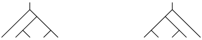
Figure 29: Rooted binary trees possessing a node with $y_{246}$, respectively $y_{135}$.

Appendix B: A finer classification in terms of trees with levels

A finer description of line soliton evolutions can be achieved by using the refinement of (rooted) binary trees to “trees with levels” [30]. Fig. 30 shows such a refinement of the second chain in Fig. 12, including also the degenerate trees at $t=t_{1345}$ and $t=t_{1235}$ which are not binary. Here we took into account that a time $t_{0}$ exists at which the two subtrees appearing between $t_{1345}$ and $t_{1235}$ have the same height, i.e. the same $y$-value. The third and the fifth tree are the two trees with levels associated with the forth tree in Fig. 30.

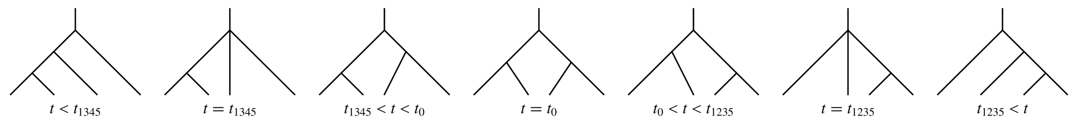
Figure 30: A finer description of the evolution as compared with that given by the second chain in Fig. 12. The third and the fifth tree are the two trees with levels associated with the tree in the middle.

Setting $t^{(5)}$ and higher variables to zero, the condition $y_{ijk}=y_{lmn}$ determines the “critical” time

$$t_{ijk;lmn}=-\frac{1}{p_{i}+p_{j}+p_{k}-p_{l}-p_{m}-p_{n}}\Big{(}c_{ijk}-c_{lmn}+[h_{2}(p_{i},p_{j},p_{k})-h_{2}(p_{l},p_{m},p_{n})]\,t^{(4)}\Big{)}\,,$$

provided that $p_{i}+p_{j}+p_{k}\neq p_{l}+p_{m}+p_{n}$.

Example B.1.

Let $M=4$. In the case considered in Fig. 30, we have $t_{0}=t_{123;345}$ and

$$t_{0}-t_{1345}=\frac{(p_{4}-p_{2})(p_{5}-p_{2})}{p_{4}-p_{1}+p_{5}-p_{2}}\,(t^{(4)}-t^{(4)}_{12345})\,,\quad t_{1235}-t_{0}=\frac{(p_{4}-p_{1})(p_{4}-p_{2})}{p_{4}-p_{1}+p_{5}-p_{2}}\,(t^{(4)}-t^{(4)}_{12345})\;.$$

Assuming $p_{1}<\cdots<p_{5}$, these expressions are both positive since the chain is only realized if $t^{(4)}>t^{(4)}_{12345}$ (right chain in Fig. 13). Furthermore,

$$x_{345}(t_{0})-x_{123}(t_{0})=\frac{(p_{4}-p_{1})(p_{4}-p_{2})(p_{5}-p_{1})(p_{5}-p_{2})}{p_{4}-p_{1}+p_{5}-p_{2}}\,(t^{(4)}-t^{(4)}_{12345})>0\;.$$

$\square$

After introduction of $t^{(5)}$, the analogous condition $t_{ijkl}=t_{mnrs}$ determines the following critical value of $t^{(4)}$,

$$t^{(4)}_{ijkl;mnrs} = -\frac{1}{p_{i}+p_{j}+p_{k}+p_{l}-p_{m}-p_{n}-p_{r}-p_{s}}\Big{(}c_{ijkl}-c_{mnrs}$$

$$+[h_{2}(p_{i},p_{j},p_{k},p_{l})-h_{2}(p_{m},p_{n},p_{r},p_{s})]\,t^{(5)}\Big{)}\,,$$

provided that $p_{i}+p_{j}+p_{k}+p_{l}\neq p_{m}+p_{n}+p_{r}+p_{s}$. See Fig. 31 for an example.

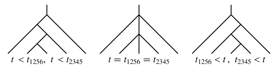
Figure 31: A transition through a coincidence of two critical times, $t_{1256}$ and $t_{2345}$, corresponding to the critical value $t^{(4)}_{1256;2345}$. This is a simultaneous rotation with respect to two different nodes.

A further useful formula is

$$t_{ijkl}-t_{mnrs}=(p_{m}+p_{n}+p_{r}+p_{s}-p_{i}-p_{j}-p_{k}-p_{l})(t^{(4)}-t^{(4)}_{ijkl;mnrs})\;.$$

Depending on the order of the $p$’s, and whether $t^{(4)}>t^{(4)}_{ijkl;mnrs}$ or $t^{(4)}<t^{(4)}_{ijkl;mnrs}$, this determines the relative order of $t_{ijkl}$ and $t_{mnrs}$.

Example B.2.

Let $M=5$. The additional critical values of $t^{(4)}$ can be used to refine Figs. 18 and 19. For $t^{(5)}<t^{(5)}_{12345}$, they have to satisfy the inequalities $t^{(4)}_{1256;2345}<t^{(4)}_{12345}<t^{(4)}_{12356}<t^{(4)}_{1236;3456}<t^{(4)}_{13456}$. Indeed, we find

$$t^{(4)}_{1236;3456}-t^{(4)}_{12356} = -\frac{(p_{4}-p_{1})(p_{4}-p_{2})}{p_{4}+p_{5}-p_{1}-p_{2}}\,(t^{(5)}-t^{(5)}_{123456})>0\,,$$

$$t^{(4)}_{13456}-t^{(4)}_{1236;3456} = -\frac{(p_{4}-p_{2})(p_{5}-p_{2})}{p_{4}+p_{5}-p_{1}-p_{2}}\,(t^{(5)}-t^{(5)}_{123456})>0\,,$$

so that $t^{(4)}_{1236;3456}$ always exists. This is not so for $t^{(4)}_{1256;2345}$. Firstly, it is only defined if $p_{1}+p_{6}\neq p_{3}+p_{4}$. Secondly,

$$t^{(4)}_{12345}-t^{(4)}_{1256;2345}=\frac{(p_{6}-p_{3})(p_{6}-p_{4})}{p_{1}+p_{6}-p_{3}-p_{4}}\,(t^{(5)}-t^{(5)}_{123456})$$

is positive only if $p_{1}+p_{6}<p_{3}+p_{4}$ holds.

For $t^{(5)}>t^{(5)}_{12345}$, the inequalities $t^{(4)}_{1256;2345}<t^{(4)}_{23456}<t^{(4)}_{12456}<t^{(4)}_{1234;1456}<t^{(4)}_{12346}$ have to be satisfied. We find

$$t^{(4)}_{1234;1456}-t^{(4)}_{12456} = \frac{(p_{5}-p_{3})(p_{6}-p_{3})}{p_{5}+p_{6}-p_{2}-p_{3}}\,(t^{(5)}-t^{(5)}_{123456})>0\,,$$

$$t^{(4)}_{12346}-t^{(4)}_{1234;1456} = \frac{(p_{5}-p_{2})(p_{5}-p_{3})}{p_{5}+p_{6}-p_{2}-p_{3}}\,(t^{(5)}-t^{(5)}_{123456})>0\,,$$

so that $t^{(4)}_{1234;1456}$ always exists. But $t^{(4)}_{1256;2345}$ only shows up if

$$t^{(4)}_{23456}-t^{(4)}_{1256;2345}=\frac{(p_{3}-p_{1})(p_{4}-p_{1})}{p_{1}+p_{6}-p_{3}-p_{4}}\,(t^{(5)}-t^{(5)}_{123456})$$

is positive, which requires $p_{1}+p_{6}>p_{3}+p_{4}$. The possible orders of the critical $t^{(4)}$-values are summarized in Table 2.

$t^{(5)}<t^{(5)}_{12345}$	$p_{1}+p_{6}<p_{3}+p_{4}$	$t^{(4)}_{1256;2345}<t^{(4)}_{12345}<t^{(4)}_{12356}<t^{(4)}_{1236;3456}<t^{(4)}_{13456}$
	$p_{1}+p_{6}>p_{3}+p_{4}$	$t^{(4)}_{12345}<t^{(4)}_{12356}<t^{(4)}_{1236;3456}<t^{(4)}_{13456}$
$t^{(5)}>t^{(5)}_{12345}$	$p_{1}+p_{6}>p_{3}+p_{4}$	$t^{(4)}_{1256;2345}<t^{(4)}_{23456}<t^{(4)}_{12456}<t^{(4)}_{1234;1456}<t^{(4)}_{12346}$
	$p_{1}+p_{6}<p_{3}+p_{4}$	$t^{(4)}_{23456}<t^{(4)}_{12456}<t^{(4)}_{1234;1456}<t^{(4)}_{12346}$

Table 2: $M=5$. The conditions under which the additional critical values $t^{(4)}_{1256;2345}$ and $t^{(4)}_{1236;3456}$, or both, are realized, and the corresponding order of critical values.

The additional critical values of $t^{(4)}$ moreover allow us to express the conditions in Table 1 under which a line soliton solution corresponds to one of the maximal chains in $\mathbb{T}_{4}$ in terms of inequalities involving only $t^{(4)}$ and its critical values. Here we use some of the above and similar expressions for the differences of critical values of $t^{(4)}$. The results are collected in Table 3.

1	$t_{1234},t_{1245},t_{2345},t_{1256},t_{2356},t_{3456}$	$t^{(4)}<\min\{t^{(4)}_{12345},t^{(4)}_{23456},t^{(4)}_{2345;1256}\}$
2	$t_{1234},t_{1245},t_{1256},t_{2345},t_{2356},t_{3456}$	$t^{(4)}_{2345;1256}<t^{(4)}<\min\{t^{(4)}_{12345},t^{(4)}_{23456}\}$
3	$t_{1234},t_{1245},t_{1256},t_{2456},t_{2346}$	$t^{(4)}_{23456}<t^{(4)}<\min\{t^{(4)}_{12345},t^{(4)}_{12456}\}$
4	$t_{1234},t_{1456},t_{1246},t_{2346}$	$t^{(4)}_{12456}<t^{(4)}<\min\{t^{(4)}_{12346},t^{(4)}_{1234;1456}\}$
5	$t_{1456},t_{1234},t_{1246},t_{2346}$	$t^{(4)}_{1234;1456}<t^{(4)}<t^{(4)}_{12346}$
6	$t_{1456},t_{1346},t_{1236}$	$t^{(4)}>\max\{t^{(4)}_{12346},t^{(4)}_{13456}\}$
7	$t_{1345},t_{1356},t_{3456},t_{1236}$	$t^{(4)}_{12345}<t^{(4)}<\min\{t^{(4)}_{12356},t^{(4)}_{23456}\}$
8	$t_{1345},t_{1356},t_{1236},t_{3456}$	$t^{(4)}_{12356}<t^{(4)}<\min\{t^{(4)}_{13456},t^{(4)}_{1236;3456}\}$
9	$t_{1345},t_{1235},t_{1256},t_{2356},t_{3456}$	$t^{(4)}_{1236;3456}<t^{(4)}<t^{(4)}_{13456}$

Table 3: The sequences of critical times determining the nine maximal chains in the Tamari lattice $\mathbb{T}_{4}$, and the conditions under which they are realized by line soliton solutions, here expressed in terms of $t^{(4)}$ and its extended set of critical values. Note that the latter are functions of $t^{(5)}$ and, depending on the value of $t^{(5)}$, they satisfy certain inequalities. See also Fig. 32.

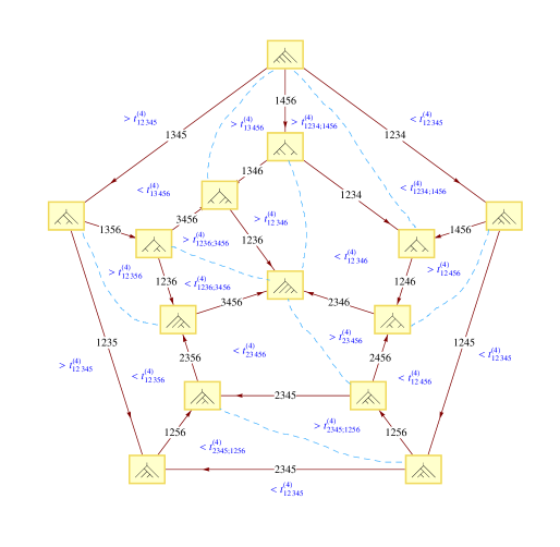
Figure 32: A representation of the Tamari lattice $\mathbb{T}_{4}$ and the conditions on $t^{(4)}$ under which the respective chains are realized by line soliton solutions. Here e.g. $>t^{(4)}_{12346}$ stands for $t^{(4)}>t^{(4)}_{12346}$. A number $ijkl$ assigned to an edge represents a critical transition time $t_{ijkl}$. On a dashed line, $t^{(4)}$ is equal to a critical value, and this corresponds to a direct transition, skipping a next neighbor on a maximal chain. For any of the additional critical values that take care of trees with levels, this is a transition in a tetragon (whereas for an ordinary critical value it takes place in a pentagon).

Appendix C: A symbolic representation of trees with levels, and a relation between permutohedra and Tamari lattices

This appendix presents some results that should also be of interest beyond the line soliton classification problem. We should stress, however, that not all statements are accompanied by a rigorous proof.

C.1 A poset structure for permutohedra

Let us assign to each node of a rooted binary tree a separate level and number the levels from top to bottom. The node on level $i$ will then be represented by the natural number $n_{i}$ if it lies on the $n_{i}$-th edge, where the edges are consecutively numbered from left to right along the level. The highest node (root node) thus always corresponds to $n_{1}=1$. In this way any rooted binary tree with levels [30] (see also Appendix Appendix B: A finer classification in terms of trees with levels) and with $r$ (internal) nodes is uniquely represented by a sequence of natural numbers $n_{1},n_{2},\ldots,n_{r}$ with $n_{i}\leq i$, $i=1,\ldots,r$, and any such sequence defines a rooted binary tree with levels. Hence we have a bijection between the set of rooted binary trees with levels and with $r$ nodes, and the set

$$\mathfrak{S}_{r}=\{\mathbf{n}=(n_{1},n_{2},\ldots,n_{r})\,|\,n_{i}\in\mathbb{N},\,n_{i}\leq i,\,i=1,\ldots,r\}\;.$$

This set has $r!$ elements. For example, the chain consisting of the first, third, fifth and last tree in Fig. 30 corresponds to the chain $(1,1,1)\longrightarrow(1,2,1)\longrightarrow(1,1,2)\longrightarrow(1,2,3)$. The left tree in Fig. 31 corresponds to $(1,1,2,2)$, the third to $(1,2,2,3)$.

On $\mathfrak{S}_{r}$ we define an action of the permutation group $\mathcal{S}_{r}$ as follows. Let $\sigma\,:\,\mathbb{N}\times\mathbb{N}\rightarrow\mathbb{N}\times\mathbb{N}$ be given by

$$\sigma(m,n)=\left\{\begin{array}[]{l}(n,m+1)\\ (n-1,m)\end{array}\right.\quad\mbox{if}\quad\begin{array}[]{l}m\geq n\\ m<n\end{array}\;.$$

Clearly, $\sigma$ is involutory: $\sigma^{2}=\mathrm{id}$. For $s=1,\ldots,r-1$, let $\sigma_{s}\,:\,\mathfrak{S}_{r}\rightarrow\mathfrak{S}_{r}$ be the map given by application of $\sigma$ to the $s$-th pair, counted from right to left, in the sequence of natural numbers defining an element of $\mathfrak{S}_{r}$, i.e.

$$\sigma_{s}(n_{1},\ldots,n_{r})=\left\{\begin{array}[]{l}(n_{1},\ldots,n_{r-s-1},n_{r-s+1},n_{r-s}+1,n_{r-s+2},\ldots,n_{r})\\ (n_{1},\ldots,n_{r-s-1},n_{r-s+1}-1,n_{r-s},n_{r-s+2},\ldots,n_{r})\end{array}\quad\mbox{if}\quad\begin{array}[]{l}n_{r-s}\geq n_{r-s+1}\\ n_{r-s}<n_{r-s+1}\end{array}\right.\;.$$

Then we have the relations

$$\sigma_{s}^{2}=\mathrm{id}\,,\qquad\sigma_{s}\,\sigma_{s+1}\,\sigma_{s}=\sigma_{s+1}\,\sigma_{s}\,\sigma_{s+1}\,,\qquad\sigma_{s}\,\sigma_{s^{\prime}}=\sigma_{s^{\prime}}\,\sigma_{s}\quad\mbox{if}\quad|s-s^{\prime}|>1\,,$$

and we have an action of the symmetric group $\mathcal{S}_{r}$ on $\mathfrak{S}_{r}$.

Let $\sigma^{H}$ be the restriction of $\sigma$ to $H=\{(n_{1},n_{2})\in\mathbb{N}\times\mathbb{N}\,|\,n_{1}\geq n_{2}\}$. Defining

$$\mathbf{n}\prec\mathbf{n}^{\prime}\qquad\mbox{if}\quad\mathbf{n}^{\prime}=\sigma^{H}_{s}(\mathbf{n})\quad\mbox{for some }\,s\,,$$

we obtain in an obvious way a partial order $\preceq$ on $\mathfrak{S}_{r}$. Then $(1,\ldots,1)$ is minimal and $(1,2,\ldots,r)$ is maximal with respect to this partial order. This results in a poset underlying the permutohedron of order $r$ [50, 51].

For what follows it is convenient to split the operation $\sigma^{H}$ into two operations $a$ and $b$, according to a split of $H$ into its diagonal part and the rest. Hence, for $m,n\in\mathbb{N}$ we have

$$a(n,n)=(n,n+1)\,,\qquad b(m,n)=(n,m+1)\quad\forall m>n\;.$$

As a consequence of their origin, the operations $a_{s}$ and $b_{s}$ satisfy the braid relation

$$a_{s}a_{s+1}a_{s}=a_{s+1}b_{s}a_{s+1}\;.$$ (C.3)

This is only defined on a subsequence of the form $n,n,n$ (with the last $n$ at position $s$, counted from the right). For $r=3$, (C.3) applied to the minimal element $(1,1,1)$ generates the whole poset underlying the permutohedron of order three, see Fig. 33. We observe that it collapses to the Tamari lattice $\mathbb{T}_{3}$ if we identify $(1,2,1)$ and $(1,1,3)$, which are related by $b_{1}$ and which are trees with levels having the same underlying rooted binary tree.

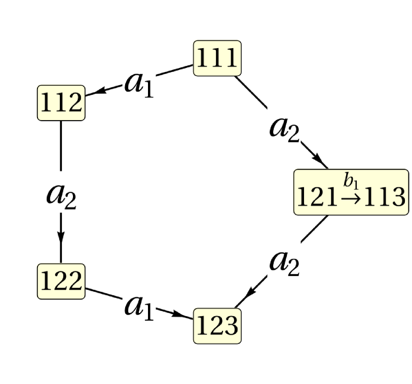
Figure 33: The Tamari lattice $\mathbb{T}_{3}$ as a collapsed permutohedron of order three. The sequences of integers at the nodes represent rooted binary trees. Here e.g. $112$ stands for $(1,1,2)\in\mathfrak{S}_{3}$.

In addition, we have the identities

$$b_{s}b_{s+1}a_{s}=a_{s+1}b_{s}b_{s+1}\,,\qquad a_{s}b_{s+1}b_{s}=b_{s+1}b_{s}a_{s+1}\,,\qquad b_{s}b_{s+1}b_{s}=b_{s+1}b_{s}b_{s+1}\,,$$ (C.4)

(where the first relation is only defined on $m,n,n$ with $m>n$, the second only on $m,m,n$ with $m>n$, and the third only on $k,m,n$ with $k>m>n$), and also

$$a_{s}a_{s^{\prime}}=a_{s^{\prime}}a_{s}\,,\quad a_{s}b_{s^{\prime}}=b_{s^{\prime}}a_{s}\,,\quad b_{s}b_{s^{\prime}}=b_{s^{\prime}}b_{s}\qquad\mbox{for}\quad|s-s^{\prime}|>1\;.$$ (C.5)

Proposition C.1.

A special maximal chain in the permutohedron poset $(\mathfrak{S}_{r},\preceq)$ is obtained by application of

$$a_{1}(a_{2}a_{1})(a_{3}a_{2}a_{1})\cdots(a_{r-2}\cdots a_{1})(a_{r-1}\cdots a_{1})$$

to the minimal element $11\ldots 1$ (with $r$ times $1$). Its length is $\frac{1}{2}(r-1)r$.

Proof: Stepwise application of $a_{r-1}\cdots a_{1}$ yields $(1,\ldots,1)\stackrel{{\scriptstyle a_{1}}}{{\longrightarrow}}(1,\ldots,1,2)\stackrel{{\scriptstyle a_{2}}}{{\longrightarrow}}(1,\ldots,1,2,2)\stackrel{{\scriptstyle a_{3}}}{{\longrightarrow}}\cdots\stackrel{{\scriptstyle a_{r-1}}}{{\longrightarrow}}(1,2,\ldots,2)$. Application of the next subsequence leads to $(1,2,\ldots,2)\stackrel{{\scriptstyle a_{1}}}{{\longrightarrow}}(1,2,\ldots,2,3)\stackrel{{\scriptstyle a_{2}}}{{\longrightarrow}}\cdots\stackrel{{\scriptstyle a_{r-2}}}{{\longrightarrow}}(1,2,3,\ldots,3)$. Continuing in this way, we finally obtain the maximal element $(1,2,\ldots,r)$. The total number of $a$’s in the sequence is $\sum_{n=1}^{r-1}n=(r-1)r/2$. $\square$

Remark C.2.

The application of an $a$ or $b$ to an element $\mathbf{n}\in\mathfrak{S}_{r}$ raises the weight $|\mathbf{n}|=n_{1}+\cdots+n_{r}$ by $1$. In order to get from $(1,\ldots,1)$, which has weight $r$, to $(1,2,\ldots,r)$ with weight $r(r+1)/2$, we need $r(r+1)/2-r=r(r-1)/2$ operations of the type $a$ or $b$. This shows that all chains in the permutohedron have the same length, namely $r(r-1)/2$.

Figure 34: A poset structure for the permutohedron of order four. Here e.g. $1211$ stands for $(1,2,1,1)\in\mathfrak{S}_{4}$.

Fig. 34 shows the permutohedron of order four (i.e. $r=4$), supplied with the poset structure introduced above. The 16 maximal chains are generated via application of the above braid relations to the sequence $a_{1}a_{2}a_{1}a_{3}a_{2}a_{1}$ that determines a maximal chain according to proposition C.1:
$a_{1}a_{2}a_{1}a_{3}a_{2}a_{1}$, $a_{1}a_{2}a_{3}a_{1}a_{2}a_{1}$, $a_{2}b_{1}a_{2}a_{3}a_{2}a_{1}$, $a_{1}a_{2}a_{3}a_{2}b_{1}a_{2}$, $(a_{2}b_{1}a_{3}b_{2}a_{3}a_{1},a_{2}a_{3}b_{1}b_{2}a_{3}a_{1})$,
$(a_{2}b_{1}a_{3}b_{2}a_{1}a_{3},a_{2}a_{3}b_{1}b_{2}a_{1}a_{3},a_{2}a_{3}a_{2}b_{1}b_{2}a_{3})$, $(a_{1}a_{3}b_{2}a_{3}b_{1}a_{2},a_{1}a_{3}b_{2}b_{1}a_{3}a_{2})$,
$(a_{3}a_{1}b_{2}a_{3}b_{1}a_{2},a_{3}a_{1}b_{2}b_{1}a_{3}a_{2},a_{3}b_{2}b_{1}a_{2}a_{3}a_{2})$, $(a_{3}b_{2}a_{3}b_{1}b_{2}a_{3},a_{3}b_{2}b_{1}a_{3}b_{2}a_{3})$.
Here we grouped those chains together that are related by a braid relation which only involves $b$’s. We shall see that also this permutohedron can be collapsed to the corresponding Tamari lattice $\mathbb{T}_{4}$.

C.2 From permutohedra to Tamari lattices

As explained in Fig. 35, the operation $a_{s}$ corresponds to a right rotation in a rooted binary tree, which is the characteristic property of a Tamari lattice.

Figure 35: The operation $a_{r-i}$ amounts to a right rotation taking place between the two levels $i$ and $i+1$. For the left tree we have $n_{i}=n_{i+1}=n$, for the right tree $n_{i}=n$ and $n_{i+1}=n+1$.

An application of $b_{s}$ does not change the respective underlying rooted binary tree, but only exchanges the associated rooted binary trees with levels, see Fig. 36.

Figure 36: The operation $b_{r-i}$ exchanges the nodes of two consecutive levels. For the left tree we have $n_{i}=n+k$, $k\in\mathbb{N}$, and $n_{i+1}=n$, for the right tree $n_{i}=n$ and $n_{i+1}=n+k+1$.

Identifying those rooted binary trees with levels that correspond to the same rooted binary tree (without levels), we can use as representative the sequence for which we also have $n_{i}\leq n_{i+1}$ (see also [52]). This defines a bijection between the set of rooted binary trees with $r$ nodes and

$$\mathfrak{Y}_{r}=\{(n_{1},n_{2},\ldots,n_{r})\,|\,n_{i}\in\mathbb{N},\,n_{i}\leq i\;\mbox{and}\;n_{i}\leq n_{i+1}\;\forall i\}\;.$$

The number of elements of this set is the Catalan number $\mathfrak{c}_{r}=\frac{1}{r+1}{2r\choose r}$ (see exercise 19 in [52]). The above partial order on $\mathfrak{S}_{r}$ induces a partial order on $\mathfrak{Y}_{r}$, and in this way a permutohedron collapses to the corresponding Tamari lattice (or associahedron, see also [53]).

Remark C.3.

In section 3.1 we described the nodes of a rooted binary tree, describing a line soliton solution at some event, as coincidences of three phases. Ordering the nodes from top to bottom and from left to right, this assigns a sequence $(i_{1},j_{1},k_{1}),\ldots,(i_{r},j_{r},k_{r})$ of ordered triples of natural numbers, $i_{m}<j_{m}<k_{m}$, to the tree. Then the sequence $i_{1},i_{2},\ldots,i_{r}$ of the first indices is precisely the sequence of natural numbers in $\mathfrak{Y}_{r}$ that characterizes the tree in the way described above. This correspondence does not extend to trees with levels.

By definition, the operation $a_{s}$ preserves $\mathfrak{S}_{r}$ (hence operates on trees with levels), but it does not preserve $\mathfrak{Y}_{r}$. We can correct this by application of operations $b_{s}$ (which are not defined on $\mathfrak{Y}_{r}$). Indeed, one can show that for any sequence $\mathbf{n}\in\mathfrak{S}_{r}\setminus\mathfrak{Y}_{r}$, there is a finite combination of $b$’s that transforms it into a sequence in $\mathfrak{Y}_{r}$.

In describing Tamari lattices, hence disregarding the refinement to trees with levels, we have to regard two sequences of $a$’s and $b$’s as equivalent if they only differ by an application of any of the rules (C.4), and those in (C.5) involving $b$’s. The restriction of the permutohedron poset to $\mathfrak{Y}_{r}$ selects those sequences in which any application of some $a_{s}$ that leads out of $\mathfrak{Y}_{r}$ is immediately corrected by $b$’s. Hence these are sequences where all $b$’s are commuted as far as possible to the right, using the braid rules that involve $b$, with the exception of (C.3). For the permutohedron of order four, the 16 maximal chains given in section C.1 reduce to 9 maximal chains, which (applied to $(1,1,1,1)$) generate the maximal chains of the Tamari lattice $\mathbb{T}_{4}$ (cf. Table 1).

Stepwise application of the special sequence of $a$’s in Proposition C.1 to the minimal element $(1,\ldots,1)$ actually generates a sequence of elements in $\mathfrak{Y}_{r}$ (see the proof of the proposition). Since the application of $a$ encodes the characteristic property of a Tamari lattice, this determines a maximal chain in a Tamari lattice. Its length is $(r-1)r/2$, and this is known to be the greatest length of a chain in $\mathbb{T}_{r}$ [54].

Proposition C.4.

A shortest maximal chain in the Tamari lattice $\mathbb{T}_{r}$ is obtained by application of

$$a_{r-1}(b_{r-2})a_{r-1}(b_{r-3}b_{r-2})a_{r-1}(b_{r-4}b_{r-3}b_{r-2})a_{r-1}\cdots a_{r-1}(b_{1}\cdots b_{r-2})a_{r-1}$$

to the minimal element $(1,\ldots,1)$ of $(\mathfrak{Y}_{r},\preceq)$.

Proof: Application of $b_{1}\cdots b_{r-2}a_{r-1}$ yields $(1,\ldots,1)\stackrel{{\scriptstyle a_{r-1}}}{{\longrightarrow}}(1,2,1,\ldots,1)\stackrel{{\scriptstyle b_{r-2}}}{{\longrightarrow}}(1,1,3,1,\ldots,1)\stackrel{{\scriptstyle b_{r-3}}}{{\longrightarrow}}(1,1,1,4,1,\ldots,1)\stackrel{{\scriptstyle b_{r-4}}}{{\longrightarrow}}\cdots\stackrel{{\scriptstyle b_{1}}}{{\longrightarrow}}(1,\ldots,1,r)$. The next subsequence $b_{2}\cdots b_{r-2}a_{r-1}$ maps $(1,\ldots,1,r)$ to $(1,\ldots,1,r-1,r)$. Continuing in this way, we finally obtain $(1,2,\ldots,r-1,r)$, the final node of $\mathbb{T}_{r}$. Hence the chain is maximal. The total number of $a$’s is $r-1$, which is known to be the shortest length of a maximal Tamari chain [54]. $\square$

Two sequences of $a$’s and $b$’s are said to belong to the same class if they differ only by an application of $a_{s}a_{s^{\prime}}=a_{s^{\prime}}a_{s}$ for $|s-s^{\prime}|>1$. In particular, for $n>3$, this rule creates further longest maximal chains from those in Propositions C.1 and C.4. The “pentagon rule” (C.3) changes a sequence (and hence a Tamari chain) in a more drastic way (since it changes the number of $a$’s).

$\mathbb{T}_{3}$ consists of two chains, each of which is a class: $a_{1}a_{2}a_{1}$ and $a_{2}b_{1}a_{2}$. For $\mathbb{T}_{4}$ there are six classes: (1) $a_{1}a_{2}a_{3}a_{1}a_{2}a_{1}$ and $a_{1}a_{2}a_{1}a_{3}a_{2}a_{1}$, (2) $a_{1}a_{2}a_{3}a_{2}b_{1}a_{2}$, (3) $a_{2}b_{1}a_{2}a_{3}a_{2}a_{1}$, (4) $a_{1}a_{3}b_{2}a_{3}b_{1}a_{2}$ and $a_{3}a_{1}b_{2}a_{3}b_{1}a_{2}$, (5) $a_{2}a_{3}a_{2}b_{1}b_{2}a_{3}$, (6) $a_{3}b_{2}a_{3}b_{1}b_{2}a_{3}$. For $\mathbb{T}_{5}$ there are 25 classes and 94 chains, see Table 4 and Fig. 28.

1	$1234123121$, $1231423121$, $1213423121$, $1231243121$, $1213243121$, $1234121321$, $1231421321$,
	$1213421321$, $1231241321$, $1213241321$, $1231214321$, $1213214321$
2	$12341232\mathbf{1}2$, $12314232\mathbf{1}2$, $12134232\mathbf{1}2$, $12312432\mathbf{1}2$, $12132432\mathbf{1}2$
3	$2\mathbf{1}23423121$, $2\mathbf{1}23243121$, $2\mathbf{1}23421321$, $2\mathbf{1}23241321$, $2\mathbf{1}23214321$
4	$12342\mathbf{1}2321$, $1232\mathbf{1}24321$, $12324\mathbf{1}2321$
5	$2\mathbf{1}232432\mathbf{1}2$, $2\mathbf{1}234232\mathbf{1}2$,
6	$123413\mathbf{2}3\mathbf{1}2$, $123431\mathbf{2}3\mathbf{1}2$, $123143\mathbf{2}3\mathbf{1}2$, $121343\mathbf{2}3\mathbf{1}2$
7	$123423\mathbf{12}31$, $123243\mathbf{12}31$, $1234231\mathbf{12}3$, $1232431\mathbf{12}3$
8	$13\mathbf{2}34\mathbf{1}2321$, $13\mathbf{2}3\mathbf{1}24321$, $31\mathbf{2}34\mathbf{1}2321$, $31\mathbf{2}3\mathbf{1}24321$
9	$23\mathbf{12}343121$, $23\mathbf{12}341321$, $23\mathbf{12}314321$, $23\mathbf{12}134321$
10	$1214\mathbf{3}4\mathbf{2}3\mathbf{1}2$, $1241\mathbf{3}4\mathbf{2}3\mathbf{1}2$, $1421\mathbf{3}4\mathbf{2}3\mathbf{1}2$, $4121\mathbf{3}4\mathbf{2}3\mathbf{1}2$, $124\mathbf{3}41\mathbf{2}3\mathbf{1}2$, $142\mathbf{3}41\mathbf{2}3\mathbf{1}2$, $412\mathbf{3}41\mathbf{2}3\mathbf{1}2$
11	$12343\mathbf{2}3\mathbf{12}3$
12	$13\mathbf{2}343\mathbf{12}31$, $13\mathbf{2}3432\mathbf{12}3$, $31\mathbf{2}343\mathbf{12}31$, $31\mathbf{2}3432\mathbf{12}3$
13	$2\mathbf{1}2343\mathbf{2}3\mathbf{1}2$
14	$23\mathbf{12}3432\mathbf{1}2$
15	$3\mathbf{2}3\mathbf{12}34321$
16	$234\mathbf{123}4121$, $2342\mathbf{123}421$, $23423\mathbf{123}41$, $234232\mathbf{123}4$, $2324\mathbf{123}421$, $23243\mathbf{123}41$, $232432\mathbf{123}4$
17	$3\mathbf{2}3432\mathbf{123}4$, $3\mathbf{2}343\mathbf{123}41$, $3\mathbf{2}34\mathbf{123}421$
18	$341\mathbf{23}4\mathbf{12}31$, $341\mathbf{23}42\mathbf{12}3$, $3413\mathbf{23}4\mathbf{12}3$, $314\mathbf{23}4\mathbf{12}31$, $314\mathbf{23}42\mathbf{12}3$, $3143\mathbf{23}4\mathbf{12}3$
19	$234\mathbf{123}42\mathbf{1}2$, $2343\mathbf{123}4\mathbf{1}2$, $2343\mathbf{2}3\mathbf{123}4$
20	$2\mathbf{1}24\mathbf{3}4\mathbf{2}3\mathbf{1}2$, $2\mathbf{1}42\mathbf{3}4\mathbf{2}3\mathbf{1}2$, $42\mathbf{1}2\mathbf{3}4\mathbf{2}3\mathbf{1}2$
21	$124\mathbf{3}4\mathbf{2}3\mathbf{12}3$, $142\mathbf{3}4\mathbf{2}3\mathbf{12}3$, $412\mathbf{3}4\mathbf{2}3\mathbf{12}3$
22	$14\mathbf{3}4\mathbf{23}4\mathbf{12}3$, $41\mathbf{3}4\mathbf{23}4\mathbf{12}3$, $4\mathbf{3}41\mathbf{23}4\mathbf{12}3$
23	$42\mathbf{3}4\mathbf{123}4\mathbf{1}2$, $42\mathbf{3}4\mathbf{2}3\mathbf{123}4$, $24\mathbf{3}4\mathbf{123}4\mathbf{1}2$, $24\mathbf{3}4\mathbf{2}3\mathbf{123}4$
24	$343\mathbf{23}4\mathbf{123}4$, $34\mathbf{23}42\mathbf{123}4$, $34\mathbf{23}4\mathbf{123}41$
25	$4\mathbf{3}4\mathbf{23}4\mathbf{123}4$

Table 4: A representation of the 25 classes of maximal chains of the Tamari lattice $\mathbb{T}_{5}$ in terms of the braid operations. Here a number $s$ in boldface stands for $b_{s}$, otherwise for $a_{s}$.

Appendix D: Tropical approximation

After the rescaling $t^{(n)}\mapsto t^{(n)}/\hbar$ and $c_{i}\mapsto c_{i}/\hbar$, with a constant $\hbar$, the class of solutions studied in sections 2, 3 and Appendix Appendix A: Some general results is given by

$$\tau=\sum_{i=1}^{M+1}e^{\theta_{i}/\hbar}\,,\qquad\theta_{i}=\sum_{n=1}^{M}p_{i}^{n}\,t^{(n)}+c_{i}\;.$$

Then we have

$$\lim_{\hbar\to 0}\hbar\,\log\tau=\lim_{\hbar\to 0}\hbar\log\Big{(}\sum_{i=1}^{M+1}e^{\theta_{i}/\hbar}\Big{)}=\max\{\theta_{1},\ldots,\theta_{M+1}\}\,,$$

applying a formula familiar in the context of tropical mathematics, and regarding $\theta_{i}$ as $\hbar$-independent. The result confirms our basic approximation formula in section 2. So far we were only interested in the (evolution of the) form of line solitons as contours in the $xy$-plane. But it is also of interest to find a good approximation for the amplitude $u$ of the KP solution e.g. at the meeting points of line soliton branches, hence at the coincidence points of phases in the tropical approximation. From

$$\phi=\hbar(\log\tau)_{x}=\frac{1}{\tau}\sum_{i=1}^{M+1}p_{i}\,e^{\theta_{i}/\hbar}=\frac{p_{k}+\sum_{i=1,i\neq k}^{M+1}p_{i}\,e^{-(\theta_{k}-\theta_{i})/\hbar}}{1+\sum_{i=1,i\neq k}^{M+1}e^{-(\theta_{k}-\theta_{i})/\hbar}}\qquad\quad k=1,\ldots,M+1\,,$$

we obtain $\lim_{\hbar\to 0}\phi=p_{k}$ in the $\theta_{k}$-region, away from coincidences of phases. At a visible coincidence $\theta_{k_{1}}=\cdots=\theta_{k_{m}}$, which is generic in the sense that it is not a coincidence of more than $m$ phases, we find $\phi=\frac{1}{m}\sum_{i=1}^{m}p_{k_{i}}$. Furthermore,

$$u = 2\hbar^{2}(\log\tau)_{xx}=2\hbar\,\phi_{x}=\frac{2}{\tau}\sum_{i=1}^{M+1}p_{i}^{2}\,e^{\theta_{i}/\hbar}-\frac{2}{\tau^{2}}\Big{(}\sum_{i=1}^{M+1}p_{i}\,e^{\theta_{i}/\hbar}\Big{)}^{2}$$

$$= \frac{2}{\tau^{2}}\sum_{1\leq i<j\leq M+1}(p_{j}-p_{i})^{2}\,e^{(\theta_{i}+\theta_{j})/\hbar}\,=\,2\,\frac{\sum_{i<j}(p_{j}-p_{i})^{2}\,e^{-(\theta_{k}+\theta_{l}-\theta_{i}-\theta_{j})/\hbar}}{\sum_{i}e^{-(\theta_{k}-\theta_{i})/\hbar}\,\sum_{j}e^{-(\theta_{l}-\theta_{j})/\hbar}}\,,$$

which implies $\lim_{\hbar\to 0}u=\frac{1}{2}(p_{k}-p_{l})^{2}$ at a visible generic coincidence $\theta_{k}=\theta_{l}$.

For an asymptotic soliton branch given by $\theta_{m}=\theta_{m+1}$ for large negative values of $y$, for $\hbar=1$ the above formula implies $u\sim\frac{1}{2}(p_{m+1}-p_{m})^{2}$ as $y\to-\infty$, which thus coincides with the tropical value. A corresponding relation also holds for the remaining asymptotic soliton branch, given by $\theta_{1}=\theta_{M+1}$, as $y\to+\infty$.

More generally, we find

$$\lim_{\hbar\to 0}u=\frac{2}{m^{2}}\sum_{1\leq i<j\leq m}(p_{k_{j}}-p_{k_{i}})^{2}\qquad\mbox{at a visible generic coincidence}\quad\theta_{k_{1}}=\cdots=\theta_{k_{m}}\;.$$

At a highest coincidence, i.e. $\theta_{1}=\cdots=\theta_{M+1}$, the tropical value is precisely the exact value (i.e. the corresponding value of $u$ for $\hbar=1$). This is not so at a (generic) visible lower coincidence. But it is clear from the above formula for $u$ that the corrections involve (only) exponentials of negative phase differences. Hence the tropical values yield a perfect approximation unless those phase differences become extremely small (which means that we are close to a higher order coincidence).

References

- [1] Zakharov V and Shabat A 1974 A scheme for integrating nonlinear equations of mathematical physics by the method of the inverse scattering transform Funct. Annal. Appl. 8 226–235
- [2] Satsuma J 1976 -soliton solution of the two-dimensional Korteweg-deVries equation J. Phys. Soc. Japan 40 286–290
- [3] Anker D and Freeman N 1978 Interpretation of three-soliton interactions in terms of resonant triads J. Fluid Mech. 87 17–31
- [4] Freeman N 1979 A two dimensional distributed soliton solution of the Korteweg-de Vries equation Proc. R. Soc. London A 366 185–204
- [5] Okhuma K and Wadati M 1983 The Kadomtsev-Petviashvili equation: the trace method and the soliton resonances J. Phys. Soc. Japan 52 749–760
- [6] Biondini G and Kodama Y 2003 On a family of solutions of the Kadomtsev-Petviashvili equation which also satisfy the Toda lattice hierarchy J. Phys. A: Math. Gen. 36 10519–10536
- [7] Kodama Y 2004 Young diagrams and -soliton solutions of the KP equation J. Phys. A: Math. Gen. 37 11169–11190
- [8] Biondini G and Chakravarty S 2006 Soliton solutions of the Kadomtsev-Petviashvili II equation J. Math. Phys. 47 033514–1–033514–26
- [9] Biondini G and Chakravarty S 2007 Elastic and inelastic line-soliton solutions of the Kadomtsev-Petviashvili II equation Math. Comp. Sim. 74 237–250
- [10] Biondini G 2007 Line soliton interactions of the Kadomtsev-Petviashvili equation Phys. Rev. Lett. 99 064103
- [11] Chakravarty S and Kodama Y 2008 Classification of the line-soliton solutions of KPII J. Phys. A: Math. Theor. 41 275209
- [12] Chakravarty S and Kodama Y 2008 A generating function for the -soliton solutions of the Kadomtsev-Petviashvili II equation Special Functions and Orthogonal Polynomials (Contemporary Mathematics vol 471) ed Dominici D and Maler R (Providence: AMS) pp 47–68
- [13] Chakravarty S and Kodama Y 2009 Soliton solutions of the KP equation and application to shallow water waves Stud. Appl. Math. 123 83–151
- [14] Chakravarty S and Kodama Y 2010 Line-soliton solutions of the KP equation AIP Conf. Proc. 1212 312–341
- [15] Chakravarty S, Lewkow T and Maruno K 2010 On the construction of the KP line-solitons and their interactions Applicable Analysis 89 529–545
- [16] Kodama Y, Oikawa M and Tsuji H 2009 Soliton solutions of the KP equation with V-shape initial waves arXiv:0904.2620
- [17] Kao C Y and Kodama Y 2010 Numerical study of the KP equation for non-periodic waves arXiv:1004.0407
- [18] Yeh H, Li W and Kodama Y 2010 Mach reflection and KP solitons in shallow water arXiv:1004.0370
- [19] Kodama Y 2010 KP solitons in shallow water arXiv:1004.4607
- [20] Tamari D 1962 The algebra of bracketings and their enumeration Nieuw Arch. Wisk. 10 131–146
- [21] Friedman H and Tamari D 1967 Problèmes d’ associativité: une structure de treillis finis induite par une loi demi-associative J. Comb. Theory 2 215–242
- [22] Huang S and Tamari D 1972 Problems of associativity: a simple proof for the lattice property of systems ordered by a semi-associative law J. Comb. Theory (A) 13 7–13
- [23] Pallo J 1986 Enumerating, ranking and unranking binary trees The Computer Journal 29 171–175
- [24] Pallo J 1987 On the rotation distance in the lattice of binary trees Inform. Process. Lett. 25 369–373
- [25] Pallo J 2003 Generating binary trees by Glivenko classes on Tamari lattices Inform. Process. Lett. 85 235–238
- [26] Pallo J 2009 Weak associativity and restricted rotation Information Process. Lett. 109 514–517
- [27] Bennett M and Birkhoff G 1994 Two families of Newman lattices Algebra Universalis 32 115–144
- [28] Geyer W 1994 On Tamari lattices Discrete Math. 133 99–122
- [29] Björner A and Wachs M 1997 Shellable nonpure complexes and posets. II Trans. AMS 349 3945–3975
- [30] Loday J L and Ronco M 1998 Hopf algebra of the planar binary trees Adv. Math. 139 293–309
- [31] Loday J L and Ronco M 2002 Order structure on the algebra of permutations and of planar binary trees J. Alg. Comb. 15 253–270
- [32] Loday J L 2002 Arithmetree J. Algebra 258 275–309
- [33] Aguiar M and Sottile F 2006 Structure of the Loday-Ronco Hopf algebra of trees J. Algebra 295 473–511
- [34] Early E 2004 Chain lengths in the Tamari lattice Annals Comb. 8 37–43
- [35] Šunić Z 2007 Tamari lattices, forests and Thompson monoids Eur. J. Comb. 28 1216–1238
- [36] Dehornoy P 2010 On the rotation distance between binary trees Adv. Math. 223 1316–1355
- [37] Miles J 1977 Obliquely interacting waves J. Fluid Mech. 79 157–169
- [38] Knuth D 1973 The Art of Computer Programming, Vol. 3: Sorting and Searching (Reading, MA: Addison-Wesley)
- [39] Sleator D, Tarjan R and Thurston W 1988 Rotation distance, triangulations, and hyperbolic geometry J. AMS 1 647–681
- [40] Caspard N and Le Conte Poly-Barbut C 2004 Tamari lattices are bounded: a new proof Technical report TR-LACL-2004-03, Université Paris-Est
- [41] Stasheff J 1998 Grafting Boardman’s cherry trees to quantum field theory arXiv:math/9803156
- [42] Stasheff J 2004 What is an operad? Notices AMS 51 630–631
- [43] Loday J L 2004 Realization of the Stasheff polytope Arch. Math. 83 267–278
- [44] Buchstaber V and Koritskaya E 2007 Quasilinear Burgers-Hopf equation and Stasheff polytopes Funct. Anal. Appl. 41 196–207
- [45] Street R 1987 The algebra of oriented simplexes J. Pure Appl. Alg. 49 283–335
- [46] Cheng E and Lauda A 2004 Higher-Dimensional Categories: an illustrated guide book (Cambridge: University of Cambridge)
- [47] Stanley R and Pitman J 2002 A polytope related to empirical distributions, plane trees, parking functions, and the associahedron Discrete Comput. Geom. 27 603–634
- [48] Speyer D and Williams L 2005 The tropical totally positive Grassmannian J. Alg. Comb. 22 189–210
- [49] Macdonald I 1995 Symmetric functions and Hall polynomials 2nd ed (Oxford: Oxford University Press)
- [50] Bowman V 1972 Permutation polyhedra SIAM J. Appl. Math. 22 580–589
- [51] Ziegler G 1995 Lectures on Polytopes (Graduate Texts in Mathematics vol 152) (Berlin: Springer)
- [52] Stanley R 1999 Enumerative Combinatorics vol 2 (Cambridge: Cambridge Univ. Press)
- [53] Tonks A 1997 Relating the associahedron and the permutohedron Operads: Proceedings of the Renaissance Conferences (Contemporary Mathematics vol 202) ed Loday J L, Stasheff J and Voronov A (Providence, RI: AMS) pp 33–36
- [54] Markowsky G 1992 Primes, irreducibles and extremal lattices Order 9 265–290
- [55] Litvinov G 2010 Tropical mathematics, idempotent analysis, classical mechanics and geometry arXiv:1005.1247
- [56] Tokihiro S, Takahashi D, Matsukidaira J and Satsuma J 1996 From soliton equations to integrable cellular automata through a limiting procedure Phys. Rev. Lett. 76 3247 – 3250